1. Introduction
The study of entrainment and the properties of the sharp interface separating turbulent from non-turbulent flow have long been subjects of research in the fluid dynamics community, with many of the concepts used tracing back to the seminal work of Corrsin & Kistler (Reference Corrsin and Kistler1954). Their prediction of a viscously dominated outer layer (viscous superlayer) at the outer edge of the turbulent/non-turbulent interface (TNTI) now seems widely accepted (e.g. Bisset, Hunt & Rogers Reference Bisset, Hunt and Rogers2002; Holzner et al. Reference Holzner, Liberzon, Nikitin, Lüthi, Kinzelbach and Tsinober2008; Holzner & Lüthi Reference Holzner and Lüthi2011; da Silva et al. Reference da Silva, Hunt, Eames and Westerweel2014; Taveira & da Silva Reference Taveira and da Silva2014) and much has been learned about the properties of the interfacial region in different flows through experiments and simulations in scenarios ranging from the simple case of shear-free turbulence (Holzner et al. Reference Holzner, Liberzon, Guala, Tsinober and Kinzelbach2006) to more complex ones such as wakes (Bisset et al. Reference Bisset, Hunt and Rogers2002), jets (Westerweel, Fukushima, Pedersen & Hunt Reference Westerweel, Fukushima, Pedersen and Hunt2009; da Silva & Rodrigo Reference da Silva and Rodrigo2010; Wolf et al. Reference Wolf, Lüthi, Holzner, Krug, Kinzelbach and Tsinober2012; van Reeuwijk & Holzner Reference van Reeuwijk and Holzner2014) and boundary layers (de Silva et al. Reference de Silva, Philip, Chauhan, Meneveau and Marusic2013; Philip et al. Reference Philip, Meneveau, de Silva and Marusic2014). Many of the results are included in a recent review on the subject by da Silva et al. (Reference da Silva, Hunt, Eames and Westerweel2014). The fact that only a very small section of this review is concerned with interfaces featuring a density stratification indicates that these flow types have received only limited attention from the community concerned with aspects of the TNTI so far. While this is understandable in view of the added complexity due to the presence of density differences, it is in striking contrast to the importance and widespread prevalence of flows featuring such a stratification. Especially in geophysical scenarios, this is a common scenario, with examples including river plumes (e.g. MacDonald, Carlson & Goodman Reference MacDonald, Carlson and Goodman2013), the deepening of the upper-ocean wind-mixed layer (e.g. Pollard, Rhines & Thompson Reference Pollard, Rhines and Thompson1972) and the very intricate case of cloud-top entrainment (e.g. Mellado Reference Mellado2010). Another flow of this category is the case of oceanic overflows that has recently received a lot of attention due to its relevance to global ocean circulation and climate models (Legg et al. Reference Legg, Briegleb, Chang, Chassignet, Danabasoglu, Ezer, Gordon, Griffies, Hallberg, Jackson, Large, Özgökmen, Peters, Price, Riemenschneider, Wu, Xu and Yang2009). In these flows denser water masses accumulate behind obstructions in shallow regions of the sea before they spill over and travel down an incline into deeper ocean basins, forming a gravity current. Oceanic overflows are found in many different locations and are observed to produce much of the deep-ocean water masses, a fact that explains their impact on a global level (Rahmstorf Reference Rahmstorf2002; Legg et al. Reference Legg, Briegleb, Chang, Chassignet, Danabasoglu, Ezer, Gordon, Griffies, Hallberg, Jackson, Large, Özgökmen, Peters, Price, Riemenschneider, Wu, Xu and Yang2009).
The underlying flow configuration of an inclined dense gravity current was first studied by Ellison & Turner (Reference Ellison and Turner1959), whose interest was triggered by a very practical problem occurring in coal mines. Numerous other investigations have dealt with the problem since then, and we refer to the very recent study of Odier, Chen & Ecke (Reference Odier, Chen and Ecke2014) for an extensive overview on the subject. Our intention here is related to the approach of Cenedese & Adduce (Reference Cenedese and Adduce2010) and Wells, Cenedese & Caulfield (Reference Wells, Cenedese and Caulfield2010), who attempt to parametrize the entrainment parameter
 $E$
(see § 2 for an exact definition) in terms of bulk properties of the flow. In this sense, we try to go a step further and relate the behaviour of
 $E$
to the local physical processes governing the entrainment rate at the interface. In other words, the goal of the present work is to study how the widely observed trend of
 $E$
to decrease with increasing stratification (e.g. Ellison & Turner Reference Ellison and Turner1959; Odier et al.
Reference Odier, Chen and Ecke2014, and references therein) is connected to changes in the small-scale processes governing the entrainment rate at the interface between turbulent and non-turbulent fluid. Such an improved understanding of the physics of the entrainment process might prove useful in the development of better entrainment parametrizations.
We present the governing equations and develop the necessary theoretical framework in § 2. The subsequent description of the experimental setup and the measurement techniques employed (§ 3) are kept short, as details have already been given elsewhere (Krug et al. Reference Krug, Holzner, Lüthi, Wolf, Kinzelbach and Tsinober2013, Reference Krug, Holzner, Lüthi, Wolf, Tsinober and Kinzelbach2014). The discussion of the results (§ 4) provides an analysis of the global flow state in a laboratory frame of reference next to an investigation in a frame of reference that is conditioned on the instantaneous TNTI position. Finally, we draw our conclusions and summarize the outcome of the study in § 5.
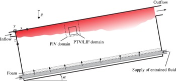
Sketch of the experimental setup. The larger dashed box indicates the approximate location of the PIV measurements; the one with solid lines roughly indicates the in-plane extent of the 3D domain.

2. Theoretical background
2.1. Governing equations
The flow considered herein features only small density differences
 ${\rm\Delta}{\it\rho}={\it\rho}_{0}-{\it\rho}$
. It is therefore well described within the Boussinesq approximation where density differences are negligible unless they are multiplied by the Earth’s gravitational acceleration,
 $\boldsymbol{g}=g\hat{\boldsymbol{z}}_{g}$
, with
 $\hat{\boldsymbol{z}}_{g}$
denoting a dimensionless unit vector pointing in the direction of gravity. Note that
 ${\rm\Delta}{\it\rho}$
is positive where the density is lower than the ambient density
 ${\it\rho}_{0}$
. The equation of motion for the gravity current then reads
 $$\begin{eqnarray}\frac{\partial \boldsymbol{u}}{\partial t}+\boldsymbol{u}\boldsymbol{\cdot }\boldsymbol{{\rm\nabla}}\boldsymbol{u}=-\boldsymbol{{\rm\nabla}}p+{\it\nu}{\rm\nabla}^{2}\boldsymbol{u}+g^{\prime }\hat{\boldsymbol{z}}_{g},\end{eqnarray}$$
where
 $g^{\prime }=g({\rm\Delta}{\it\rho}/{\it\rho}_{0})$
is the reduced gravitational acceleration and
 ${\it\nu}$
is the kinematic viscosity. The transport equation for the density difference is given by
 $$\begin{eqnarray}\frac{\partial {\rm\Delta}{\it\rho}}{\partial t}+\boldsymbol{u}\boldsymbol{\cdot }\boldsymbol{{\rm\nabla}}{\rm\Delta}{\it\rho}=\mathscr{D}\,{\rm\nabla}^{2}{\rm\Delta}{\it\rho},\end{eqnarray}$$
with
 $\mathscr{D}$
denoting the molecular diffusivity of the stratifying agent. The relevant dimensionless parameters for this case formed with inflow parameters (indicated by subscript zero) are the Reynolds number
 $\mathit{Re}_{0}=U_{0}d/{\it\nu}$
, the Richardson number
 $\mathit{Ri}_{0}=g_{0}^{\prime }d/U_{0}^{2}$
and the Schmidt number
 $\mathit{Sc}={\it\nu}/\mathscr{D}$
.
The coordinate system is fixed to the centre-plane at the inlet (see figure 1) with the
 $x$
-axis pointing in the streamwise direction, while the
 $z$
-coordinate measures the distance from the wall and the
 $y$
-axis runs along the spanwise direction. The velocity components are denoted by
 $u$
,
 $v$
and
 $w$
in the
 $x$
-,
 $y$
- and
 $z$
-directions, respectively. Where appropriate, index notation is used, with
 $x_{i}$
indicating the coordinate directions and
 $u_{i}$
the corresponding velocity components.
2.2. Global entrainment parametrization
Following the widely used Morton–Taylor–Turner (MTT) entrainment hypothesis (Morton, Taylor & Turner Reference Morton, Taylor and Turner1956), the induced global entrainment velocity
 $u_{e}$
is directly proportional to some velocity
 $U^{\ast }$
characterizing the bulk flow:
 $u_{e}=EU^{\ast }$
. The exact value of the entrainment parameter
 $E$
depends on the choice of
 $U^{\ast }$
. While the mean centreline velocity is usually used for jets, it is more common (e.g. Ellison & Turner Reference Ellison and Turner1959) to use the top-hat velocity scale in gravity currents, which is defined along with the top-hat width
 $h$
by
 $$\begin{eqnarray}U_{T}h=\int _{z=0}^{\infty }u\text{d}z\quad \text{and}\quad U_{T}^{2}h=\int _{z=0}^{\infty }u^{2}\text{d}z.\end{eqnarray}$$
The advantage of the formulation in top-hat scales is that the product of
 $U_{T}$
and
 $h$
equals the local volume flux. Therefore, using mass conservation, the entrainment parameter can be obtained simply from
 $$\begin{eqnarray}E=\frac{1}{U_{T}}\frac{\partial (U_{T}h)}{\partial x}.\end{eqnarray}$$
2.3. Local entrainment velocity
The turbulent boundary is commonly defined based on a threshold of enstrophy
 ${\it\omega}^{2}={\bf\omega}\boldsymbol{\cdot }{\bf\omega}$
, where the vorticity vector is given by
 ${\bf\omega}=\boldsymbol{{\rm\nabla}}\times \boldsymbol{u}$
. It seems therefore natural to express entrainment in terms of enstrophy isosurfaces as done by Holzner & Lüthi (Reference Holzner and Lüthi2011), who defined a local entrainment velocity,
 $v_{n}$
, as the velocity with which an enstrophy isosurface element moves relative to the fluid. They showed that the local entrainment velocity is given by
 $$\begin{eqnarray}v_{n}=-\frac{1}{|\boldsymbol{{\rm\nabla}}{\it\omega}^{2}|}\frac{\text{D}{\it\omega}^{2}}{\text{D}t}.\end{eqnarray}$$
Based on the enstrophy transport equation, which for the case of a flow with small density differences reads
 $$\begin{eqnarray}\frac{1}{2}\frac{\text{D}{\it\omega}^{2}}{\text{D}t}={\it\omega}_{i}{\it\omega}_{j}s_{ij}+{\it\nu}{\it\omega}_{i}{\rm\nabla}^{2}{\it\omega}_{i}+{\it\epsilon}_{ijk}{\it\omega}_{i}\frac{\partial g_{k}^{\prime }}{\partial x_{j}},\end{eqnarray}$$
 $v_{n}$
can be split up into different contributions according to
 $$\begin{eqnarray}v_{n}=-\frac{2{\it\omega}_{i}{\it\omega}_{j}s_{ij}}{|\boldsymbol{{\rm\nabla}}{\it\omega}^{2}|}-\frac{2{\it\nu}{\it\omega}_{i}{\rm\nabla}^{2}{\it\omega}_{i}}{|\boldsymbol{{\rm\nabla}}{\it\omega}^{2}|}-\frac{2{\it\epsilon}_{ijk}{\it\omega}_{i}\displaystyle \frac{\partial g_{k}^{\prime }}{\partial x_{j}}}{|\boldsymbol{{\rm\nabla}}{\it\omega}^{2}|}=v_{n}^{\mathscr{I}}+v_{n}^{\mathscr{V}}+v_{n}^{\mathscr{B}}.\end{eqnarray}$$
From left to right, the three terms on the right-hand side of (2.7) are due to an inviscid term (denoted by
 $v_{n}^{\mathscr{I}}$
), a viscous term (
 $v_{n}^{\mathscr{V}}$
) and a contribution due to the baroclinic torque (
 $v_{n}^{\mathscr{B}}$
), which is peculiar for flows featuring a density difference.
2.4. Relation between global and local approach to entrainment
The entrained volume flux through an instantaneous enstrophy isosurface with surface area
 $A_{{\it\eta}}$
, on the one hand, is given by the integral
 $$\begin{eqnarray}Q_{{\it\omega}}=\int _{A_{{\it\eta}}}v_{n}\text{d}A,\end{eqnarray}$$
where
 $A_{{\it\eta}}$
expresses the instantaneous surface area of the enstrophy isosurface and the subscript
 ${\it\eta}$
is used to emphasize that this is a contorted surface with convolutions over a spectrum of scales. On the other hand, the entrained volume flux in the top-hat approach is given by
 $$\begin{eqnarray}Q_{th}=u_{e}A_{0}=EU_{T}A_{0},\end{eqnarray}$$
with
 $A_{0}$
denoting the projected surface area, i.e. the area of the
 $xy$
-plane of the measurement volume. The mean interface position when conditioning on enstrophy is found at a position
 $h_{{\it\omega}}$
that tends to be further away from the wall than the top-hat thickness
 $h$
. The fluxes defined in (2.8) and (2.9) are related by the ratio of
 $h$
and
 $h_{{\it\omega}}$
(van Reeuwijk & Holzner Reference van Reeuwijk and Holzner2014) according to
 $$\begin{eqnarray}Q_{{\it\omega}}=\frac{h_{{\it\omega}}}{h}Q_{th}.\end{eqnarray}$$
This relationship offers a different approach to determine the entrainment constant via a threshold based on enstrophy:
 $$\begin{eqnarray}E=\frac{Q_{{\it\omega}}}{U_{T}A_{0}}\frac{h}{h_{{\it\omega}}}.\end{eqnarray}$$
The new expression links the MTT approach to the direct physical mechanisms responsible for the vorticity transfer at the interface, namely the viscous diffusion of enstrophy (aided by enstrophy production) at small scales that operates across a large convoluted surface and hence allows us to study how the dynamics at the TNTI influence the entrainment parameter.
3. Experiments
3.1. Setup
The experiments in the present study were conducted in a gravity current facility that has already been presented in Krug et al. (Reference Krug, Holzner, Lüthi, Wolf, Kinzelbach and Tsinober2013). The description is therefore kept to a minimum here and we refer to the previous publication for further details. The setup is sketched in figure 1. It consists of a tank (2 m long and 0.5 m high and wide) that is tilted against the horizontal plane by an angle of
 ${\it\alpha}=10^{\circ }$
. The gravity current is realized by letting lighter index-matched fluid flow continuously along the top of this tank. The turbulence level at the inflow is enhanced by means of an array of flapping grids. The inflow rate is measured and kept constant to within 2 %. Entrained denser fluid is gently resupplied along the bottom of the tank to prevent large-scale circulation in the flow domain. The density difference between the two fluids is achieved by using refractive-index-matched water-based solutions of sodium chloride and ethanol. A similar experiment was recently conducted by Odier, Chen & Ecke (Reference Odier, Chen and Ecke2012).
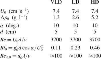
In this paper, we present results for two different flow cases that differ only in their initial density difference at the inlet,
 ${\rm\Delta}{\it\rho}_{0}$
. The two cases will be abbreviated by LD (for ‘lower density difference’) and HD (‘higher density difference’) from here on. For HD,
 ${\rm\Delta}{\it\rho}_{0}=5.2~\text{g}~\text{l}^{-1}$
, which is twice the value of
 ${\rm\Delta}{\it\rho}_{0}$
for LD. An overview of all the flow parameters determined at the inflow is presented in table 1. Both the inflow Reynolds number,
 $\mathit{Re}_{0}$
, and the inflow Richardson number,
 $\mathit{Ri}_{0}$
, are computed using the inlet height,
 $d$
, and a mean inflow velocity,
 $U_{0}$
, that is defined as the ratio of the inflow rate and the cross-section of the inflow opening. As the flow evolves, the Richardson number changes and its value at the measurement position may therefore differ from the reported inflow value. Since our density measurements are confined to a domain that is smaller than the width of the gravity current, we cannot determine the actual global
 $\mathit{Ri}$
at the location of the measurements accurately. However, this shortcoming does not interfere with our objective in this work, which is to relate variations of the entrainment rate to changes in the flow processes at the interface and not necessarily to establish a relation between the entrainment rate and
 $\mathit{Ri}$
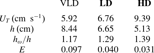
. Note that the LD case resembles the parameter set investigated in Krug et al. (Reference Krug, Holzner, Lüthi, Wolf, Kinzelbach and Tsinober2013). Table 1 additionally lists the parameters for a third flow case labelled ‘VLD’ for ‘very low density difference’. In this case the initial density difference was half the one of the LD case. However, it was found that for this case the turbulent flow region then extended beyond our measurement domain for significant times, which may bias some of the statistics. We decided, however, to include at least some of the data as they seemed useful in underlining some of the trends observed in the other two cases.
Inflow parameters for the two main flow cases (bold face) considered; additionally data for a third case (VLD) is included (see text for details).

3.2. Measurements
Results of two types of measurements will be presented in the following. In order to capture the entire flow field spanning from the wall to the unmixed region, particle image velocimetry (PIV) measurements were performed on a domain whose approximate location is indicated by the dashed box in figure 1. The field of view was located approximately 50 cm away from the inlet and covered roughly 15 cm in the streamwise and wall-normal directions. The spatial resolution for both cases was approximately equivalent to
 $4{\it\eta}$
, with
 ${\it\eta}$
being the Kolmogorov length scale; the effective temporal resolution is 83 Hz. Further specifications of the PIV setup can be found in Krug et al. (Reference Krug, Holzner, Lüthi, Wolf, Kinzelbach and Tsinober2013). At least 10 000 frames (corresponding to 40 s or 59 shear time scales
 $d/U_{0}$
) were evaluated for each flow case to ensure good statistical convergence of the two-dimensional (2D) velocity data.
Moreover, simultaneous three-dimensional (3D) data of both the velocity field and the density field were obtained on a smaller subdomain, indicated by the solid box in figure 1 through a combination of scanning particle tracking velocimetry (PTV) and scanning laser-induced fluorescence (LIF). This measurement technique and the postprocessing scheme employed are described in great detail in Krug et al. (Reference Krug, Holzner, Lüthi, Wolf, Tsinober and Kinzelbach2014). The paper also presents an analysis of the measurement accuracies using checks based on kinematic relations and the continuity equation. The size of the measurement volume is
 $4~\text{cm}\times 4~\text{cm}\times 2~\text{cm}$
in streamwise, wall-normal and spanwise directions, respectively. PTV is based on following tracer particles in time and space and therefore initially yields a Lagrangian data set. For analyses that require an Eulerian setting, this data set is interpolated on a grid with a spacing of 1.5 mm, which is equivalent to a distance of approximately
 $5{\it\eta}$
for both flow cases. As we demonstrate in Krug et al. (Reference Krug, Holzner, Lüthi, Wolf, Tsinober and Kinzelbach2014), we are further able to obtain the full velocity gradient tensor from the PTV measurements with good accuracy. The density measurements are indirect via the concentration of a tracer dye that is initially mixed into only one of the two fluids. The 3D density information is obtained by scanning the volume with a laser sheet and stacking in-plane results acquired at different depth positions. Hence, there is a resolution difference between the in-plane directions (streamwise/wall-normal directions) and the scanned direction (spanwise). After a coarse graining in the image plane (see Krug et al. (Reference Krug, Holzner, Lüthi, Wolf, Tsinober and Kinzelbach2014) for details), the resulting spatial resolutions are 0.4 mm in
 $x$
- and
 $z$
-directions and 1 mm in
 $y$
-direction. With a dynamic pixel intensity range of approximately 130, the nominal resolution of the LIF system is
 $0.008{\rm\Delta}{\it\rho}_{0}$
. For results where joint statistics of velocity and density data are used, the density field is filtered to match the resolution of the velocity field. Velocity and density data are recorded simultaneously and resolved temporally at 200 Hz. The duration of single runs was limited by the storage capabilities of the cameras to 2.7 s. The presented data set consists of a total of 40 runs per flow case, which is equivalent to more than 100 s of recording or approximately
 $150d/U_{0}$
.
4. Results
4.1. Global analysis
The PIV measurements allow investigation of bulk flow properties at the measurement location (approximately
 $10d$
from the inlet). Previous investigations in the same (Krug et al.
Reference Krug, Holzner, Lüthi, Wolf, Kinzelbach and Tsinober2013) and similar (Ellison & Turner Reference Ellison and Turner1959; Chen et al.
Reference Chen, Odier, Rivera and Ecke2007; Odier et al.
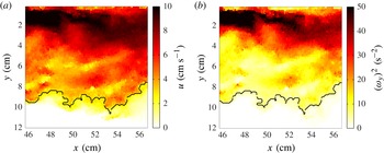
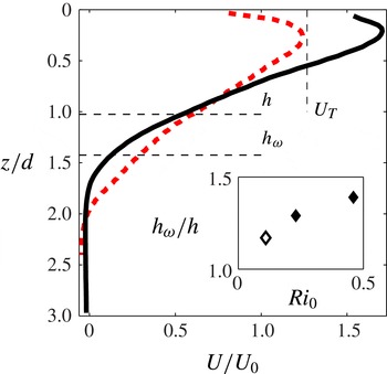
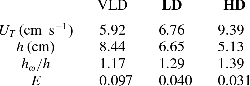
Reference Odier, Chen and Ecke2014) setups indicate that the flow at this stage has already adjusted from the inflow conditions and reached an equilibrium state. Sample illustrations of instantaneous distributions of streamwise velocity and the enstrophy component available from PIV taken from the LD case are displayed in figure 2. The most prominent differences in the flow evolution of the two cases are easily identified from mean profiles averaged in time and
 $x$
-direction shown in figure 3. In general, the flow is faster and less spread out in the HD case compared to the LD profile. While in the HD case an increase of
 $u$
by more than 50 % with respect to
 $U_{0}$
is observed in the region close to the wall, the LD profile shows only a slight increase in the same area. Going further away from the wall, the velocity maximum is followed by a region of almost constant velocity gradient in both flows until the mean streamwise velocity drops to zero. This part of the flow is commonly denoted as ‘mixing region’. The HD flow features a higher velocity gradient in this region such that the extent of the mixing region is smaller and the velocity reaches zero closer to the wall than in the LD case. The previously described differences between the two flows are also reflected in the results for
 $h$
and
 $U_{T}$
as defined by (2.3a,b
), which are included in table 2. As would be expected, we find that
 $U_{T}^{HD}>U_{T}^{LD}$
and
 $h^{HD}<h^{LD}$
.
Instantaneous snapshots of (a) the streamwise velocity,
 $u$
, and (b) the square of the out-of-plane vorticity component,
 $({\it\omega}_{y})^{2}$
, as obtained from the PIV measurements of the LD case. The black line indicates the instantaneous location of
 $h_{{\it\omega}}$
.

Velocity profiles obtained from PIV measurements approximately
 $10d$
away from the inlet: LD, dashed (red) line; HD, solid (black) line. Thin horizontal dashed lines labelled
 $h$
and
 $h_{{\it\omega}}$
, respectively, indicate the location of the top-hat width and the mean location of the enstrophy interface for HD. The short vertical line indicates
 $U_{T}$
for HD. The inset shows the ratio
 $h_{{\it\omega}}/h$
for different inflow Richardson numbers.

To give an impression of how the top-hat quantities are related to the velocity profiles, the locations of
 $h$
and
 $h_{{\it\omega}}$
are included in figure 3 for the HD case. The mean position of the enstrophy isosurface,
 $h_{{\it\omega}}$
, was obtained from the PIV data using a threshold on the only available enstrophy component of
 ${\it\omega}_{y}^{2}=1~\text{s}^{-2}\approx 0.46(U_{0}/d)^{2}$
. Instantaneous samples of
 $h_{{\it\omega}}$
are included as the black lines in the snapshots of figure 2; for details on the procedure used to determine the location of
 $h_{{\it\omega}}$
, we refer to Krug et al. (Reference Krug, Holzner, Lüthi, Wolf, Kinzelbach and Tsinober2013). As can be seen from figure 3, the top-hat width is located within the mixing region, while the enstrophy interface marks the outer edge of the flow profile. The inset in figure 3 displays the ratio
 $h_{{\it\omega}}/h$
as a function of
 $\mathit{Ri}_{0}$
for the two flows considered (filled symbols). Additionally, it shows a data point for the VLD case (open symbol). As mentioned above, the enstrophy isosurface is located outside the measurement domain for significant times for this very low
 $\mathit{Ri}_{0}$
and the value of
 $h_{{\it\omega}}$
is thus likely to be slightly underestimated. However, this should not affect the observed trend of increasing
 $h_{{\it\omega}}/h$
with increasing
 $\mathit{Ri}_{0}$
. The trend is consistent with the observation made earlier that
 $h_{{\it\omega}}$
is located at the outer edge of the mean velocity profile. As the profiles get more compact and the velocity gradient in the mixing region increases with increasing
 $\mathit{Ri}_{0}$
, the relative distance between
 $h$
and
 $h_{{\it\omega}}$
increases.
From the streamwise development of the top-hat scales within the measurement domain, the entrainment parameter
 $E$
can be determined from (2.4) (see Krug et al. (Reference Krug, Holzner, Lüthi, Wolf, Kinzelbach and Tsinober2013) for details). From the variation of the results when taking only half of the available data, we estimate the error of this procedure to be within
 $\pm 0.002$
in
 $E$
. This analysis yields
 $E=0.031$
and
 $E=0.040$
for the HD and LD cases, respectively, which is consistent with the expected trend of decreasing
 $E$
for increasing stratification. The numbers can be put into perspective by considering the fact that the values for
 $E$
reported for unstratified flows are around
 $E\approx 0.08{-}0.1$
(e.g. Ellison & Turner Reference Ellison and Turner1959) marking the distinct impact of the stratification in the gravity currents. An overview of different flow parameters determined from PIV including data for the VLD flow is presented in table 2.
Overview of flow parameters determined from PIV measurements for the two main flow cases (bold face) and the VLD parameters.
4.2. Interface dynamics
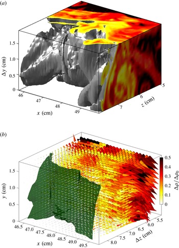
The goal of this section is to study the flow dynamics in the vicinity of the TNTI of the gravity current. For this purpose, we employ data obtained from the combined scanning PTV/LIF measurements. Samples of these measurements taken with the higher initial density difference are displayed in figure 4.
(a) Illustration of an instantaneous density field obtained from the experiment in the HD case. The grey isosurface is placed at
 ${\it\rho}^{\prime }/{\rm\Delta}{\it\rho}_{0}=8\,\%$
, with slices illustrating the density variation within the gravity current flow. (b) Combination of velocity and density data. The local velocity vectors are represented by the direction and size of the cones. Their greyscale (colour) illustrates the local normalized density difference. The largest cones in the turbulent region represent velocities around
 $10~\text{cm}~\text{s}^{-1}$
. The dark grey (green) isosurface marks the position where the local enstrophy value is equal to
 $5~\text{s}^{-2}$
. The greyscale (colour) bar in (b) applies to both panels.

The instantaneous interface position fluctuates considerably in time such that conventional averaging in laboratory coordinates would smear out the interfacial statistics. It has proven beneficial (e.g. Bisset et al.
Reference Bisset, Hunt and Rogers2002; Holzner et al.
Reference Holzner, Liberzon, Nikitin, Lüthi, Kinzelbach and Tsinober2008; Westerweel et al.
Reference Westerweel, Fukushima, Pedersen and Hunt2009) to employ a coordinate frame that is conditioned on the instantaneous interface position,
 $\boldsymbol{x}_{if}$
. We define the interface position as the location of the enstrophy isosurface where
 ${\it\omega}^{2}={\it\omega}_{th}^{2}=5~\text{s}^{-2}$
in both flows. This threshold value lies just above the noise level of our data. A sample isosurface is included in the cone plot of figure 4(b). We define a new coordinate,
 $\tilde{z}$
, whose origin is attached to the interface and which runs along the direction of the local normal vector of the isosurface given by
 $\boldsymbol{n}=\boldsymbol{{\rm\nabla}}{\it\omega}^{2}/|\boldsymbol{{\rm\nabla}}{\it\omega}^{2}|$
. Since the gradient of enstrophy points towards the turbulent zone, positive values of
 $\tilde{z}$
indicate regions within the turbulent zone while negative values are found in the irrotational region. Quantities averaged in the conditioned frame of reference are labelled with a tilde or angular brackets where appropriate.
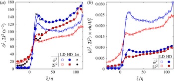
Figure 5(a) shows conditioned profiles of enstrophy and strain. Similar to other flow cases (Bisset et al.
Reference Bisset, Hunt and Rogers2002; Holzner et al.
Reference Holzner, Liberzon, Nikitin, Lüthi, Kinzelbach and Tsinober2008; Westerweel et al.
Reference Westerweel, Fukushima, Pedersen and Hunt2009; Wolf et al.
Reference Wolf, Holzner, Lüthi, Krug, Kinzelbach and Tsinober2013), the increase in
 $\tilde{{\it\omega}}^{2}$
at
 $\tilde{z}=0$
is steep, with only the noise level present in the irrotational zone. The values of enstrophy are generally higher for the flow with the higher initial density difference. Deeper inside the turbulent zone, enstrophy values of approximately
 $120~\text{s}^{-2}$
(LD) and
 $160~\text{s}^{-2}$
(HD) are reached, such that the chosen threshold value,
 ${\it\omega}_{th}^{2}$
, relates to 4 % (LD) and 3 % (HD) of the mean enstrophy value in the turbulent zone. Owing to the steep rise of the enstrophy profiles, changes of
 ${\it\omega}_{th}^{2}$
have only little impact on the location of the interface. In fully developed homogeneous turbulence, the averages of
 ${\it\omega}^{2}$
and
 $2s^{2}$
, where the strain is given by
 $s^{2}=s_{ij}s_{ij}$
and
 $s_{ij}=(\partial u_{i}/\partial x_{j}+\partial u_{j}/\partial x_{i})/2$
is the rate-of-strain tensor, are expected to be of equal magnitude (Tsinober Reference Tsinober2009). As figure 5(a) shows, this state is approached only for values of
 $\tilde{z}/{\it\eta}>100$
. Unlike for the enstrophy profiles, significant values of strain are also found in the region
 $\tilde{z}/{\it\eta}<0$
, showing the existence of strain due to irrotational velocity fluctuations there. Additionally, figure 5(a) displays data measured in a round jet at
 $\mathit{Re}=5000$
of Wolf et al. (Reference Wolf, Holzner, Lüthi, Krug, Kinzelbach and Tsinober2013). It is interesting to note that, even in this unstratified case, the profiles of enstrophy and strain are very similar in the proximity of the TNTI. While the good agreement of the jet data with the HD case is merely a coincidence, it exemplifies the general trend that the stratification effects on these profiles are relatively small. The same profiles of enstrophy and strain are plotted again for the two gravity currents in figure 5(b), but this time normalized by
 $U_{T}^{3}/({\it\nu}h)$
, a scale related to the respective energy flux. This normalization reveals that the LD case is much more effective than the HD case in converting shear into turbulence intensity, as can be concluded from the fact that the situation in the turbulent region is now reversed in comparison to figure 5(a) and the LD case now attains values that are about three times as high as the ones for the HD flow.
(a) Conditioned profiles of
 $\tilde{{\it\omega}}^{2}$
(blue circles) and
 $2\tilde{s}^{2}$
(red squares) for the two flow cases: HD, full symbols; LD, open symbols. (b) Same as (a) but normalized by
 $U_{T}^{3}/({\it\nu}h)$
. Additional data from a round jet by Wolf et al. (Reference Wolf, Holzner, Lüthi, Krug, Kinzelbach and Tsinober2013) are included, with crosses and stars marking
 $\tilde{{\it\omega}}^{2}$
and
 $2\tilde{s}^{2}$
, respectively.

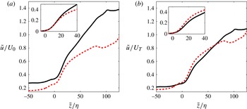
Sharp variations are known to exist at the interface for quantities such as the streamwise velocity displayed in figure 6 (Westerweel et al.
Reference Westerweel, Fukushima, Pedersen and Hunt2009). In part because of the effects of finite measurement resolution, these so-called jumps manifest themselves as regions of steeper gradients in the interval
 $0\leqslant \tilde{z}/{\it\eta}\leqslant 15$
. The velocity profiles are plotted twice, normalized once by the inflow velocity
 $U_{0}$
(figure 6
a) and once by the top-hat velocity
 $U_{T}$
(figure 6
b). The comparison between the two shows that the profiles of
 $\tilde{u}$
nearly collapse deeper in the turbulent zone when scaled by
 $U_{T}$
, whereas this does not seem to hold for the velocity jump. Judging from the insets of figure 6, the velocity jumps are better matched when normalized by
 $U_{0}$
, or equivalently when given in dimensional units. There is a very close agreement in the inset of figure 6(a) for the two flow cases between
 $\tilde{z}/{\it\eta}=0$
and
 $\tilde{z}/{\it\eta}=10$
before the velocity curves drift slightly apart, with the HD case attaining higher values when normalized with
 $U_{0}$
and lower values when normalized with
 $U_{T}$
, respectively.
(a) Conditioned profile of the streamwise velocity normalized by
 $U_{0}$
: HD, solid (black) line; LD, dashed (red) line. The inset shows a magnification of the interfacial zone with the profiles shifted such that their value at the origin equals zero. (b) Same as (a) but normalized by
 $U_{T}$
.

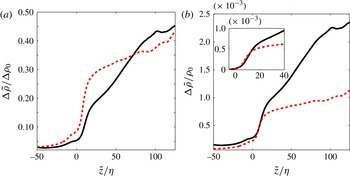
The conditioned profile of the density difference is shown in figure 7. Neglecting the effects of molecular diffusion, the distribution of a passive scalar would be expected to scale solely with the initial concentration. The fact that a collapse of the density curves is not observed when normalizing by the respective initial density difference (cf. figure 7
a) points towards the active role played by
 ${\rm\Delta}{\it\rho}$
in the interfacial dynamics. Similar to what was observed for the streamwise velocity, the density jumps also collapse nicely for
 $0\leqslant \tilde{z}/{\it\eta}\leqslant 10$
when scaled by a quantity that is equal for both cases, in this case the background density
 ${\it\rho}_{0}$
(see figure 7
b). The density gradient, and therefore the level of stratification in the turbulent zone away from the interface, is significantly stronger for the HD case.
Conditioned density difference normalized by (a) the respective initial density difference and (b) the background density
 ${\it\rho}_{0}$
: HD, solid (black) line; LD, dashed (red) line. The inset in (b) shows a magnification of the interfacial region with the profiles shifted such that they match at
 $\tilde{z}=0$
.

The gradient Richardson number
 $\mathit{Ri}_{g}=N^{2}/(\partial u/\partial z_{g})^{2}$
is a dimensionless number that relates the competing effects of stratification and shear locally. Note that
 $z_{g}$
denotes a coordinate that runs parallel to the direction of gravitational acceleration. Buoyancy effects enter the computation of
 $\mathit{Ri}_{g}$
in the form of the Brunt–Väisälä frequency,
 $N^{2}=(g/{\it\rho}_{0})(\partial ({\rm\Delta}{\it\rho})/\partial z_{g})$
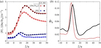
. Figure 8 presents the two components of the conditioned gradient Richardson number,
 $\langle N\rangle$
and
 $|\langle \partial u/\partial z_{g}\rangle |$
, separately (figure 8
a) as well as
 $\tilde{\mathit{Ri}}_{g}$
itself (figure 8
b). Consistent with the observations made for the density and velocity jumps in figures 6 and 7, the two quantities displayed in figure 8(a) agree closely in the interval
 $0\leqslant \hat{z}/{\it\eta}\leqslant 10$
for the two flow cases. Both stratification and shear are observed to exhibit significant peaks in the vicinity of the TNTI, with higher peak values for the higher initial density difference. The maxima of
 $\langle N\rangle$
are located around
 $\tilde{z}/{\it\eta}=10$
and therefore closer to the interface than those for
 $|\langle \partial u/\partial z_{g}\rangle |$
, which are found between
 $\tilde{z}/{\it\eta}=15$
and
 $\tilde{z}/{\it\eta}=20$
. The resulting conditioned profiles of
 $\tilde{\mathit{Ri}}_{g}$
have a distinct maximum around
 $\tilde{z}/{\it\eta}=10$
, indicating a stratification-dominated region. The HD profile additionally exhibits a minimum around
 $\tilde{z}/{\it\eta}=20$
, the same location as the maximum shear for this case, and keeps increasing further in the turbulent zone. A similar, but much less pronounced, behaviour is also observed for the LD case. The stratification peaks in figure 8(b) are of the same strength at
 $\tilde{\mathit{Ri}}_{g}\approx 0.1$
, apparently independent of the initial density differences. A natural explanation for this striking observation, along with the previously observed similarities in the jumps, would be the existence of a certain equilibrium state of stratification and shear in the proximity of the TNTI. The idea behind such an assumption will be elaborated further in the next section.
(a) Plots of
 $\langle N\rangle$
(blue squares) and
 $|\langle \partial u/\partial z_{g}\rangle |$
(red circles) for the two flow cases: LD, open symbols; HD, filled symbols. (b) Conditioned profiles of the gradient Richardson number
 $\tilde{\mathit{Ri}}_{g}=\langle N^{2}\rangle /\langle \partial u/\partial z_{g}\rangle ^{2}$
: HD, solid (black) line; LD, dashed (red) line).

Joint p.d.f.s of the density gradient
 $\partial {\it\rho}/\partial z_{g}$
and the velocity gradient
 $\partial u/\partial z_{g}$
binned into three different regions relative to the interface, namely (a,d) non-turbulent zone (
 $-15\leqslant \tilde{z}/{\it\eta}\leqslant -5$
), (b,e) interfacial region (
 $0\leqslant \tilde{z}/{\it\eta}\leqslant 25$
), and (c, f) turbulent region (
 $35\leqslant \tilde{z}/{\it\eta}\leqslant 45$
), for (a–c) LD and (d–f) HD. The greyscale (colour) bars in (c) and ( f), respectively, apply to the entire row. The arrows indicate the local direction and magnitude of
 $\text{D}(\partial {\it\rho}/\partial z_{g})/\text{D}t$
and
 $\text{D}(\partial u/\partial z_{g})/\text{D}t$
in the vertical and horizontal directions, respectively. Grey lines in (b) and ( e) represent isolines of the gradient Richardson number
 $\mathit{Ri}_{g}=(g\partial {\it\rho}/\partial z_{g})/(\partial u/\partial z_{g})^{2}$
.

4.3. Gradient transport analysis
To investigate the dynamics of the stratification and shear in the interfacial region, the transport equations for the density gradient
 $\partial {\it\rho}/\partial z_{g}$
and the velocity gradient
 $\partial u/\partial z_{g}$
are studied, where again
 $z_{g}$
denotes a projection along the direction of gravity. The evolution of these two terms is governed by the transport equations for the density gradient,
 $$\begin{eqnarray}\frac{\text{D}{\it\rho}_{,i}}{\text{D}t}=-{\it\rho}_{,k}\frac{\partial u_{k}}{\partial x_{i}}+\mathscr{D}\,{\rm\nabla}^{2}{\it\rho}_{,i},\end{eqnarray}$$
where
 $\mathscr{D}$
is the molecular diffusion of the stratifying agent, and the one for the velocity gradients,
 $A_{ij}=\partial u_{i}/\partial x_{j}$
,
 $$\begin{eqnarray}\frac{\text{D}A_{ij}}{\text{D}t}=-A_{ik}A_{kj}-\frac{\partial p}{\partial x_{i}\partial x_{j}}+{\it\nu}{\rm\nabla}^{2}A_{ij}+\frac{\partial g_{i}^{\prime }}{\partial x_{j}}.\end{eqnarray}$$
The equation for the density gradient features only two terms on the right-hand side: the first one is due to the interaction of the velocity and the density gradient, and the second one is due to molecular diffusion. The evolution of the velocity gradient is influenced by inviscid interaction of velocity gradients (first term) and viscous effects (third term). Additionally, there is a term (
 $\partial p/\partial x_{i}\partial x_{j}$
) that captures the nonlocal influence of the pressure forces. The last term in the evolution equation of the velocity gradient tensor is due to buoyancy. However, just like the corresponding term in the evolution equation for vorticity (see § 4.4.1), its contributions were seen to be small compared to the other terms.
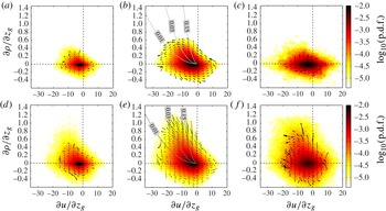
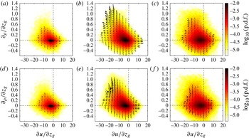
Joint p.d.f.s of the density gradient
 $\partial {\it\rho}/\partial z_{g}$
and the velocity gradient
 $\partial u/\partial z_{g}$
for the HD case with the same binning as in figure 9. The velocity vectors in (a–c) show the effect of the first (inviscid) terms on the right-hand side of (4.1) and (4.2) only. Vectors in (d–f) show the effect of the diffusion term of (4.1) in the vertical direction and the combined contributions of the non-local, viscous and baroclinic terms of (4.2) in the horizontal direction.

Figure 9 shows joint probability density functions (p.d.f.s) of
 $\partial u/\partial z_{g}$
and
 $\partial {\it\rho}/\partial z_{g}$
in the non-turbulent region, the interfacial zone and inside the turbulent region for the two flow cases. Note that, when going away from the top wall, the density tends to increase whereas the streamwise velocity decreases. Consequently, the velocity gradient,
 $\partial u/\partial z_{g}$
, is predominantly negative while the density gradient,
 $\partial {\it\rho}/\partial z_{g}$
, is mostly positive. Primarily in the interfacial region (figure 9
b,e), negative values of
 $\partial u/\partial z_{g}$
and positive
 $\partial {\it\rho}/\partial z_{g}$
appear to be correlated, which is indicated by a somewhat elongated shape of the joint p.d.f. for these values. This observation points towards a dynamical interplay between the two gradients in this zone. Especially in the interfacial and turbulent regions, the joint p.d.f. for the HD case (lower line in figure 9) is somewhat wider spread, which implies more vigorous fluctuations around the mean state for this flow.
The vectors in the same figure allow us to evaluate the dynamics in terms of the gradient evolutions
 $\text{D}(\partial {\it\rho}/\partial z_{g})/\text{D}t$
and
 $\text{D}(\partial u/\partial z_{g})/\text{D}t$
that were determined along Lagrangian trajectories. The traces of a cyclic pattern can be found most prominently in the second quadrant (i.e.
 $\partial u/\partial z_{g}<0$
and
 $\partial {\it\rho}/\partial z_{g}>0$
) of the plots displaying data from the interfacial zone (figure 9
b,e).
In the course of this cycle, weaker velocity and density gradients grow up to a point where shear reaches a certain limit, above which at first the stratification and eventually also the shear tend to decrease. The isolines of
 $\mathit{Ri}_{g}$
in figure 9(b,e) indicate that, even during the growth period of the gradients,
 $\mathit{Ri}_{g}$
decreases. The turning point of the gradient evolution roughly coincides with
 $\mathit{Ri}_{g}=0.03$
in both cases and the gradient Richardson number decreases further as the gradients decrease. We note that in some locations vectors are strongly pointing outwards rather than tangential to the probability contours, which would locally lead to diverging dynamics and not an accurate delineation of a cycle. We attribute this to both limited statistics and finite experimental accuracy rather than to a genuine physical effect. The reason is that the joint distribution is statistically steady and ideally the divergence of the probability flux is zero (see Chevillard et al.
Reference Chevillard, Meneveau, Biferale and Toschi2008). The nature of the cyclic pattern is further dissected in figure 10, which presents the terms on the right-hand side of (4.1) and (4.2) separately. The inviscid terms (figure 10
a–c) are computed directly, whereas the remaining terms, i.e. the diffusion term for the density gradient and the combined contribution of the pressure and viscous diffusion for the velocity gradient evolution (figure 10
d–f), are obtained from the experimentally available terms (i.e. the inviscid terms and the material derivatives) using the balance in (4.1) and (4.2), respectively. There is a prominent trend for the inviscid effects to amplify gradients, whereas the remaining terms act to reduce stratification and shear. Even though traces of this trend are present in all three regions, it is far more pronounced in the interfacial region. In the third and fourth quadrants (i.e. below the abscissa axis), the density gradients are unstable and the flow returns to lower gradient magnitudes more quickly, leaving
 $\partial {\it\rho}/\partial z_{g}$
and
 $\partial u/\partial z_{g}$
largely uncorrelated also in the interfacial region.
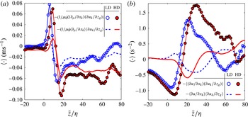
Conditioned profile of the averaged inviscid terms (a)
 $-(1/{\it\rho}_{0})\langle (\partial {\it\rho}/\partial x_{k})(\partial u_{k}/\partial z_{g})\rangle$
and (b)
 $-\langle (\partial u/\partial x_{k})(\partial u_{k}/\partial z_{g})\rangle$
that appear in the transport equations (4.1) and (4.2) for
 $\partial {\it\rho}/\partial z_{g}$
and
 $\partial u/\partial z_{g}$
, respectively (HD case, full red symbols; LD case, open blue symbols). Lines without symbols represent the respective contributions of the mean quantities (a)
 $-(1/{\it\rho}_{0})\langle \partial {\it\rho}/\partial x_{k}\rangle \langle \partial u_{k}/\partial z_{g}\rangle$
and (b)
 $-\langle \partial u/\partial x_{k}\rangle \langle \partial u_{k}/\partial z_{g}\rangle$
(HD, solid red line; LD, dashed blue line).

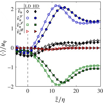
The conditionally averaged local entrainment velocity,
 $\tilde{v}_{n}$
(black diamonds), and its components
 $\tilde{v}_{n}^{\mathscr{V}}$
(blue circles),
 $\tilde{v}_{n}^{\mathscr{I}}$
(green squares) and
 $\tilde{v}_{n}^{\mathscr{B}}$
(red triangles) for the LD case (open symbols) and HD case (filled symbols). All velocities are normalized by the respective Kolmogorov velocity,
 $u_{{\it\eta}}$
, for the two cases that are given in table 3.

A reason why the cyclical behaviour is most prominent in the interfacial region is found in figure 11, where the average effects of the inviscid terms of (4.1) and (4.2) are presented. It is important to recall here that the mean density (velocity) gradients in the mixing region are positive (negative) throughout. Hence, their magnitude is amplified if
 $-(1/{\it\rho}_{0})\langle (\partial {\it\rho}/\partial x_{k})(\partial u_{k}/\partial z_{g})\rangle >0$
and
 $-\langle (\partial u/\partial x_{k})(\partial u_{k}/\partial z_{g})\rangle <0$
, respectively. With reference to figure 11, both conditions are met only in the interfacial zone. It is therefore only in the proximity of the interface that the inviscid terms act on average to increase the magnitude of the respective mean gradients. Without this restoring force, the equilibrium could not be sustained leading to a gradual decrease of the magnitude of the mean gradients as evidenced by the streamwise evolution of mean density and velocity profiles averaged in laboratory coordinates reported in Odier et al. (Reference Odier, Chen and Ecke2014). It is noteworthy that the inviscid amplification of the mean gradients in the interfacial regions is driven by the fluctuations for both quantities. This is evident from the fact that the product of the means in figure 11 is significantly smaller than the mean of the products of the gradients for the ranges of
 $\tilde{z}$
in which the mean gradients are amplified through inviscid interaction. The physical picture that evolves from the synopsis of the observations of a mean cyclic evolution in this section is the following. The flow tends to amplify stable density gradients as well as shear in the proximity of the interface through the inviscid interaction of velocity and density gradients (cf. figure 11). During this process, the relative importance of the stable stratification decreases continually as evidenced by a decreasing gradient Richardson number. At low enough
 $\mathit{Ri}_{g}$
– the present data suggest a value around
 $\mathit{Ri}_{g}\approx 0.03$
– the dominant shear gives rise to more intense turbulence, which in turn increases vertical stirring. As a consequence of the increased mixing, molecular effects are intensified (cf. figure 10
e), limiting the buildup of stratification and shear (for the case of shear with the help of pressure) and ultimately even leading to a reduction of these gradients reverting the flow state to the original condition. The fact that the peaks of the joint p.d.f.s in figure 9(b,e) are found at similar locations, along with the earlier observation of closely agreeing flow dynamics in the interfacial region (e.g. the matching peaks for
 $\tilde{\mathit{Ri}}_{g}$
in figure 8
b), suggest that the interplay of stratification and shear evolves around a common equilibrium state in both flow cases. The amplitude of fluctuations around this mean state appears to be larger for the HD case, which is reflected by a larger spread of the joint p.d.f. of
 $\partial {\it\rho}/\partial z_{g}$
and
 $\partial u/\partial z_{g}$
for HD in figure 9(e) compared to the LD case (figure 9
b). The existence of a common local flow state implies that the flow situation at the TNTI tends to be locally independent of the initial level of stratification.
4.4. Entrainment analysis
4.4.1. Local entrainment velocity
Figure 12 provides information on the behaviour of the conditional average of the local entrainment velocity defined in (2.5) in the proximity of the interface. It shows the averaged profiles of
 $\tilde{v}_{n}$
and its components as defined in (2.7). Note that, owing to the fact that the normal vector is pointing into the turbulent region, negative values of
 $\tilde{v}_{n}$
imply outward movement of the enstrophy isosurface. One of the striking features of this plot is certainly that the baroclinic torque
 $\tilde{v}_{n}^{\mathscr{B}}$
is small throughout for both flow cases and does not contribute significantly either at the interface or around
 $\tilde{z}/{\it\eta}=10$
where the stratification is strongest (cf. figure 8
a). Further, it is found that
 $\tilde{v}_{n}^{\mathscr{V}}$
contributes strongly to the expansion of the turbulent zone. The ratios of
 $\tilde{v}_{n}^{\mathscr{V}}/\tilde{v}_{n}$
at
 $\tilde{z}=0$
are 0.4 for the LD case and slightly higher at 0.6 for the HD flow, which places the chosen threshold in the ‘buffer region’ defined by van Reeuwijk & Holzner (Reference van Reeuwijk and Holzner2014) in which both the viscous and the inviscid components produce an outward movement of the isosurface. The difference in the ratios is in line with the fact that the mean enstrophy level in the turbulent region is higher in the HD case (cf. figure 5
a). This implies a lower relative threshold for this flow since the threshold
 ${\it\omega}_{th}^{2}$
is kept equal in absolute numbers, such that the interface lies closer to the ‘viscous superlayer’, where the contribution of
 $\tilde{v}_{n}^{\mathscr{I}}$
vanishes (van Reeuwijk & Holzner Reference van Reeuwijk and Holzner2014). It seems likely that this difference in the relative thresholds is also the reason for the slight shift in
 $\tilde{z}$
for the curves that is most prominently observed for
 $\tilde{v}_{n}^{\mathscr{I}}$
and
 $\tilde{v}_{n}^{\mathscr{V}}$
. Apart from this shift, the profiles for the two flow cases considered agree closely. This is not surprising in view of the fact that it was observed earlier in § 4.2 how closely the flow states match in the interfacial region. Deeper inside the turbulent zone, the viscous component of
 $\tilde{v_{n}}$
changes sign and attains positive values whereas
 $\tilde{v}_{n}^{\mathscr{I}}$
decreases further. The baroclinic torque remains negligible throughout and there is a net inward relative propagation velocity (i.e. a slightly positive
 $\tilde{v}_{n}$
) for enstrophy isosurfaces with mean locations at
 $\tilde{z}/{\it\eta}>10$
. These trends are consistent with observations in turbulent jets (Wolf et al.
Reference Wolf, Holzner, Lüthi, Krug, Kinzelbach and Tsinober2013; van Reeuwijk & Holzner Reference van Reeuwijk and Holzner2014).
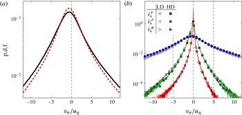
Further insight into the characteristics of the local entrainment velocity is provided by the p.d.f.s of
 $v_{n}$
at the interface in figure 13(a) and its components in figure 13(b). The p.d.f.s of
 $v_{n}$
clearly feature negative means and match closely for the two different flows apart from a slightly wider distribution in the HD case. Hence, also the respective mean values of
 $-0.39u_{{\it\eta}}$
for LD and
 $-0.41u_{{\it\eta}}$
for HD are in good agreement. Consistent with earlier findings in zero-mean shear turbulence (Holzner & Lüthi Reference Holzner and Lüthi2011) and a round jet (Wolf et al.
Reference Wolf, Lüthi, Holzner, Krug, Kinzelbach and Tsinober2012, Reference Wolf, Holzner, Lüthi, Krug, Kinzelbach and Tsinober2013), these means as well as the standard deviations are of the order of the Kolmogorov velocity scale. Moreover, these results are close to values reported in a round jet of
 $\tilde{v}_{n}/u_{{\it\eta}}=-0.26$
at a lower (
 $\mathit{Re}=2000$
) and
 $\tilde{v}_{n}/u_{{\it\eta}}=-0.50$
at a higher (
 $\mathit{Re}=5000$
) Reynolds number (Wolf et al.
Reference Wolf, Holzner, Lüthi, Krug, Kinzelbach and Tsinober2013). The plot of the p.d.f.s of the velocity components in figure 13(b) shows only negligible differences between the two flows. In agreement with results in other flows (Holzner & Lüthi Reference Holzner and Lüthi2011; Wolf et al.
Reference Wolf, Lüthi, Holzner, Krug, Kinzelbach and Tsinober2012, Reference Wolf, Holzner, Lüthi, Krug, Kinzelbach and Tsinober2013), it is found that the distribution of the viscous component is much wider than those of the remaining components. It is further noteworthy that the baroclinic torque is generally small and not only negligible in the mean (cf. figure 12). However, the distribution of
 $v_{n}^{\mathscr{B}}$
is skewed towards negative values such that the term acts on average to propagate the isosurface outwards.
(a) The p.d.f.s of
 $v_{n}$
at the interface location for the two flow cases: LD, dashed (red) line; HD, solid (black) line. (b) The p.d.f.s of the components of
 $v_{n}$
at the interface, namely
 $v_{n}^{\mathscr{V}}$
(blue circles),
 $v_{n}^{\mathscr{I}}$
(green squares) and
 $v_{n}^{\mathscr{B}}$
(red triangles), for the LD case (open symbols) and HD case (filled symbols).

4.4.2. Stratification effects on the bulk entrainment parameter
Using the 3D data, it is possible to evaluate the entrainment parameter from (2.11). We obtain
 $E=0.031$
for LD and
 $E=0.040$
for HD, which is in excellent agreement with the values calculated from the PIV measurements reported earlier in § 4.1. Moreover, the good agreement between results derived from 2D and 3D data validates the assumption that spanwise variations are negligible in the mean flow. On top of that, the fact that the value obtained for the LD case additionally compares favourably to recent experimental results of Odier et al. (Reference Odier, Chen and Ecke2014) further establishes the credibility of the present measurements.
Expressing the volume flux
 $Q_{{\it\omega}}$
over the enstrophy isosurface by using the mean values of the convoluted isosurface and of the local entrainment velocity, yielding
 $Q_{{\it\omega}}=\langle v_{N}\rangle \langle A_{{\it\eta}}\rangle$
and substituting into (2.11), we obtain the following expression for the entrainment parameter:
 $$\begin{eqnarray}E=\frac{\langle v_{n}\rangle }{U_{T}}\frac{\langle A_{{\it\eta}}\rangle }{A_{0}}\frac{h}{h_{{\it\omega}}}.\end{eqnarray}$$
By means of this formulation, it is now possible to study the effects of different stratification levels on the factors on the right-hand side of (4.3) individually. As outlined in § 4.1, the mean velocity profiles of the flow tend to become more spread out with decreasing
 $\mathit{Ri}_{0}$
. This implies a decrease for the top-hat velocity
 $U_{T}$
with decreasing
 $\mathit{Ri}_{0}$
. At the same time,
 $h/h_{{\it\omega}}$
increases for weaker initial stratification levels (see figure 2
a and discussion thereof). The
 $\mathit{Ri}_{0}$
dependence of
 $U_{T}$
is observed to be stronger than that of the ratio of
 $h$
and
 $h_{{\it\omega}}$
. Thus, the overall trend of the factors representing global flow scales in (4.3) is to decrease
 $E$
as
 $\mathit{Ri}_{0}$
is increased.
The local entrainment velocity was evaluated in detail in the previous subsection (§ 4.4.1) and, in accordance with the consistent flow features close to the interface, no significant differences were found between the two flows investigated. The mean values measured in the gravity currents are – if at all – only weakly influenced by stratification, which is evident from the fact that the values in the gravity current are in the range of those measured in a jet flow at similar Reynolds numbers. For the present stratification levels, the component of
 $v_{n}$
involving density gradients was observed to be negligible throughout such that the close agreement between mean values in stratified and unstratified flows seems very plausible.
Of all the factors in (4.3), the largest influence of density effects appears to be on the ratio of the surface area of the convoluted isosurface over the projected surface,
 $A_{{\it\eta}}/A_{0}$
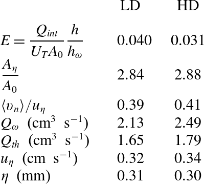
. There is no appreciable difference between the two flow cases investigated, where the values agree closely at 2.88 (HD) and 2.84 (LD, see also table 3) but the stratification effect becomes evident when comparing to flows without density differences. In unstratified flow cases, Sreenivasan, Ramshankar & Meneveau (Reference Sreenivasan, Ramshankar and Meneveau1989) and more recently de Silva et al. (Reference de Silva, Philip, Chauhan, Meneveau and Marusic2013) established a fractal scaling of the surface area
 $A$
of the TNTI evaluated at a scale
 $r$
according to
 $A(r)\propto r^{2-D_{f}}$
. They consistently report values of
 $D_{f}\approx 2+(1/3)$
for the fractal dimension. Consequently we obtain
 $A_{{\it\eta}}/A_{0}=({\it\eta}/L)^{-1/3}$
as an estimate based on the scale separation between Kolmogorov scale,
 ${\it\eta}$
, and integral scale,
 $L$
. Even with a very conservative estimate of
 ${\it\eta}/L=0.01$
, we get
 $A_{{\it\eta}}/A_{0}\approx 4.64$
for the unstratified case, which is significantly higher than the values we measure in the gravity currents. It therefore seems likely that the main effect of the stratification, which principally affects the larger scales, is to reduce the convolutedness of the interface, thereby setting a lower entrainment rate.
Coming back to the comparison of the two flow cases considered here, it is remarkable that the entrained volume flux,
 $Q_{{\it\omega}}$
, is very similar in dimensional numbers for the two stratification levels (the value for HD is in fact even slightly higher, cf. table 3). As a consequence, the trend of decreasing
 $E$
for increasing
 $\mathit{Ri}_{0}$
is almost uniquely caused by the tendency of
 $U_{T}$
to increase with
 $\mathit{Ri}_{0}$
.
Overview of entrainment parameters determined from PTV measurements.

5. Conclusion
The experimental investigation presented here explores the small-scale features of the interfacial region between turbulent and non-turbulent flow regions in an inclined dense gravity current. The goal is to analyse the behaviour of the widely used entrainment parameter
 $E$
in relation to the physical processes governing the entrainment rate at the interface. For this purpose, a relation between the entrained flux across an enstrophy isosurface and the entrainment parameter expressed in top-hat scales was established. The effect of different stratification levels was analysed on the basis of experimental data for two flow cases with different levels of initial stratification. The two cases are abbreviated by LD (for ‘lower density difference’) and HD (‘higher density difference’). The large-scale structure of the respective velocity fields is studied by means of PIV, while 3D measurements of the density and velocity through PTV and LIF on a smaller domain capturing the interfacial region allow us to investigate the small-scale features there.
The entrainment parameter was obtained independently in the two measurements with very good agreement. The values obtained (
 $E=0.03$
for HD and
 $E=0.04$
for LD) further match literature data well and are significantly lower than those commonly obtained in unstratified flows. The dominant effect of the large-scale flow state on
 $E$
was found to be an increase of the top-hat velocity,
 $U_{T}$
, with increasing
 $\mathit{Ri}_{0}$
owing to a more compact mean velocity profile.
An analysis of the interfacial dynamics revealed jumps in the density and velocity profiles that are generally slightly larger for the HD case. However, there exists a region
 $0<\tilde{z}/{\it\eta}<10$
where the profiles for the two flows match closely, which is most prominently reflected by identical peaks of the gradient Richardson number around
 $\tilde{z}/{\it\eta}=10$
. We offer a possible explanation for this observation in terms of a cyclic evolution of shear and stratification around a common local equilibrium state for the two flow cases. The cycle involves inviscid amplification terms of the evolution equations for density and velocity gradients, on the one hand. On the other hand, once the gradients are amplified, stirring intensifies molecular processes, which – along with the pressure – are seen to decrease gradients of velocity and density. Consistent with the locally similar flow state, small-scale properties at the interface, such as the local entrainment velocity, do not differ significantly. The component of
 $v_{n}$
due to the baroclinic torque was observed not to contribute significantly for either stratification level.
A major impact of the stratification on the entrainment process is noticed indirectly on the ratio of the surface area of an enstrophy isosurface at low thresholds. In both flows investigated here, we obtain
 $A_{{\it\eta}}/A_{0}=2.8$
, which is considerably lower than corresponding estimates from fractal scaling in unstratified flows. According to these, the ratio is reduced by approximately a factor of 2, and therefore similar to the reduction in
 $E$
between unstratified flows and the gravity currents investigated here. Thus the differences in the surface area seem to account for much of the reduction in
 $E$
compared to flows without stable density gradients. In contrast, the smaller variation in
 $E$
between the two gravity currents compared here is mostly due to differences in
 $U_{T}$
as the entrained volume flux across the enstrophy isosurface is almost equal.
Acknowledgements
The first author would like to thank E. Schuh and D. Pilav for helping out with the experiments. This work was supported by the Swiss National Science Foundation (SNF) under project number 200021/132567.