Nomenclature
-
 $\rho $
-
density (kg/m3)
-
$t\;$
-
time (s)
-
$u$
-
velocity (m/s)
-
$p$
-
static pressure (Pa)
-
${\tau_{ij}}$
-
viscous stress tensor
-
$e$
-
energy (J/kg)
-
${k_t}$
,
${k_v}$
-
thermal conductivity (w/(m·K))
-
$T$
-
static temperature (K)
-
$Q$
-
energy convert (J/kg)
-
${\tau_\alpha }$
-
translational-vibrational relaxation time (s)
-
$X$
-
mole fraction
-
$M$
-
molecular weight (kg/mol)
-
$\theta $
-
characteristic vibrational temperature (T)
-
$Y$
-
mass fraction
-
$g$
-
degeneracy
-
$R$
-
universal gas constant (J/(mol·K))
-
$D$
-
mass diffusion coefficient (m2/s)
-
$S$
-
source term of the chemical reaction (kg/(m3·s))
-
$C$
-
molar concentration (mol/m3)
-
$\eta $
-
rate exponent
-
$\Gamma $
-
third body efficiency
-
${k_{}}$
-
reaction rate coefficient ((m3/mol)n-1/s)
-
$A$
-
pre-factor ((m3/mol)n-1/s)
-
$\beta $
-
temperature index
-
${T_c}$
-
reaction control temperature (K)
-
${K_{eq}}$
-
equilibrium constant
-
$k$
-
turbulent kinetic energy (m2/s2)
-
$\mu $
-
dynamic viscosity (kg/(m·s))
-
${\mu_t}$
-
turbulent viscosity (kg/(m·s))
-
$\omega $
-
specific dissipation rate (1/s)
-
$\sigma $
-
turbulent Prandtl number
-
$\kappa $
-
reacting volume fraction
-
${\tau^*}$
-
time scale
-
${t_c}$
-
chemistry time scale
-
${t_{mix}}$
-
mixing time scale
-
$\eta $
-
combustion efficiency
-
$\dot m$
-
mass flow rate (kg/s)
-
$F$
-
net thrust (N)


Subscripts
-
$i$
,
$j$
-
direction
-
$t$
-
translation
-
$v$
-
rotation
-
$reac$
,
$c$
-
chemical reaction
-
$\alpha $
,
$\gamma $
,
$j$
-
species
-
$m$
-
vibrational mode
-
$r$
-
reaction
-
$f$
-
forward
-
$b$
-
backward
-
$a$
-
activation


1.0 Introduction
Supersonic vehicles represent the advanced technology in the aerospace field [Reference Morelli and Derry1], with significant application prospects. Currently, various countries worldwide attach great importance to the development of this technology [Reference Xu and Shi2, Reference Viviani and Pezzella3]. The high-Mach scramjets can fully utilise the atmospheric oxygen to enhance flight efficiency and are expected to become excellent power sources for future reusable earth-to-space round trips [Reference Sandeep4–Reference Curran6]. However, the significant characteristics of high temperature and high speed in high Mach scramjet, new technical challenges are posed for engine design [Reference Xu and Shi2, Reference Viviani and Pezzella3, Reference Jose, Raj, Dewang and Sharma7].
In the scramjet combustor, the intense shock waves and turbulent characteristics can alter the thermodynamic state of the compressible gas, including density, temperature, pressure and also affect the mixing state of fuel and air [Reference Anderson8]. These phenomena excite the vibrational modes of molecules and produce thermal non-equilibrium effects, namely the translational-vibrational non-equilibrium (hereinafter referred to as vibrational non-equilibrium). These effects alter the thermodynamics, the transport properties of the flow field and chemical reaction rates, significantly impacting the performance of high-speed engines [Reference Moreira, Wolf and Azevedo9, Reference Zeng, Yuan, Zhao and Chen10]. Additionally, at elevated temperatures, air undergoes further chemical reactions, such as the dissociation and ionisation of oxygen and nitrogen. The resulting radicals, electrons, ions and other species engage in subsequent reactions with fuel-related species, producing a chemical non-equilibrium effect [Reference Shang and Yan11–Reference Zhao, Yang, Wang, Zheng and Zhou13]. The two effects mentioned earlier are collectively referred to as the thermochemical non-equilibrium effect, which is worth focusing on and researching.
The experimental research on thermochemical non-equilibrium flow is conducted by aeronautical research institutes and requires specialised high-precision equipment, such as shock-wave wind tunnels [Reference Dunn, Moller and Steele14, Reference Jiang, Hu, Wang and Han15]. Compared to experiments, the cost of computational fluid dynamics (CFD) numerical simulations is usually lower, particularly for cases requiring stringent conditions and high-precision measurements. Numerical simulations can provide comprehensive information about the flow field, including regions that are difficult to measure experimentally.
To quantify the effects of translational-vibrational non-equilibrium in numerical simulations, Park [Reference Park16] proposed the two-temperature model. This model introduces a vibrational-electronic temperature to describe vibrational and electronic energy, and uses a translational-rotational temperature to describe translational and rotational energy. After years of development, the two-temperature model has become the most common method for simulating vibrational non-equilibrium. In addition, researchers have developed three-temperature models and multi-temperature models [Reference Park and Lee17]. For possible chemical reactions that may occur in the combustor, Dunn and Kang [Reference Dunn and Kang18] first proposed air-reaction mechanisms of 11 species, including dissociation and ionisation reactions. Park [Reference Park19] and Gupta [Reference Gupta, Yos and Thompson20] also proposed air reaction mechanisms of 11 species in their respective studies. Meanwhile, Park [Reference Park19] proposed the
 ${T_t}$
-
 ${T_v}$
model for calculating the rate constants of chemical reactions by combining the two-temperature model.
Hydrogen (H2) has the advantages of high specific energy and high reactivity [Reference Cecere, Giacomazzi and Ingenito21, Reference Lebrouhi, Djoupo, Lamrani, Benabdelaziz and Kousksou22] and is an important fuel in high-speed aircraft. To describe H2 combustion accurately, Jachimowski [Reference Jachimowski23] proposed mechanisms for H2 combustion in air (13 species and 33 reactions). John et al. [Reference Evans and Schexnayder24] proposed a mechanism of 12 species and 25 reactions. These mechanisms include the dissociation of N2 and formation of NO. Liang et al. [Reference Liang, He, Ji and Zhao25] proposed a functional weight analysis (FW) to identify the dominant mechanism of oscillatory combustion in MILD combustion systems. By quantifying the dynamic influence of interspecies interactions, they successfully constructed the framework mechanism of methane and propane capable of predicting oscillatory behaviour. Ai et al. [Reference Ai, Liang, Ji and Zhao26] used the above-mentioned FW analysis method to reveal the dynamic mechanism of unstable combustion in the NH3/H2 mixed combustion system, identified that three feedback cycles, namely hydrogen chain branching, NH2 dehydrogenation oxidation, and NOX-DeNOX, are the key factors driving oscillatory combustion, and explained their association with the increase in NOx emissions.
To perform non-equilibrium numerical simulation, the researchers developed relevant programs. Based on the open-source platform OpenFOAM, Casseau et al. [Reference Casseau27] developed a non-equilibrium CFD solver named hy2Foam, which was verified in various zero-dimensional adiabatic simulations [Reference Casseau, Palharini, Scanlon and Brown28] and multi-dimensional analyses [Reference Casseau, Espinoza, Scanlon and Brown29]. This solver can be used for secondary development applications. Ao et al. [Reference Ao, Wu, Lu, Ji and Fan30] developed the HiSCFOAM-NonE solver to simulate non-equilibrium high-speed combustion in the HyShot II scramjet, in which different degrees of non-equilibrium zones. Zidane et al. [Reference Zidane, Haoui, Sellam and Bouyahiaoui31] independently developed the HRF code to simulate H2 combustion in rocket nozzle flows. Yao [Reference Yao32] used a self-developed combination software package Amber to study the flow combustion in a full-size hydrogen-fueled scramjet at Mach 12, finding that while the thermochemical non-equilibrium effect enhanced air-fuel mixing, it reduced combustion efficiency and the engine thrust. ANSYS Fluent [33] has introduced a two-temperature model in recent years and coupled it with chemical reactions.
A substantial body of research has focused on the thermochemical non-equilibrium effects in scramjets. Gehre et al. [Reference Gehre, Wheatley and Boyce34] conducted CFD simulations of the T3 shock tunnel with a nozzle of inflow Mach 6 under both thermal equilibrium and non-equilibrium conditions, with a focus on comparing the differences between ground shock-tunnel tests and actual flight conditions. Fiévet et al. [Reference Fiévet, Voelkel, Koo, Raman and Varghese35] used high-resolution numerical simulations to study the effects of thermal non-equilibrium on ignition and stability in a scramjet combustor. They found that the initial temperature difference generated by the non-equilibrium flow significantly altered the ignition position. In subsequent studies, Fiévet et al. [Reference Fiévet and Raman36] applied a multi-temperature model to investigate the translational-vibrational non-equilibrium of flow in the isolation section at an inflow Mach 1.9 condition, without chemical reactions. The results showed that the non-equilibrium effects caused slow relaxation of N2, significantly increasing the pseudo-shock structure length. Koo et al. [Reference Koo, Raman and Varghese37] used direct numerical simulation to study the effects of thermal non-equilibrium on flame structure in supersonic flow, finding that non-equilibrium phenomena at low vibrational temperatures could inhibit combustion. Wang et al. [Reference Wang, Zhuo, Dai and Sun38] studied the thermochemical non-equilibrium effect of the nozzle of a Mach 10 scramjet engine, and the results indicate that vibrational relaxation and chemical reactions interact in the flow-field, which has a significant impact on engine operation.
The DLR combustor is a commonly used strut combustor in numerical simulations [Reference Oevermann39–Reference Genin and Menon41]. Weidman et al. [Reference Alff, Brummund, Clauss, Oschwald, Sender and Waidmann42, Reference Gucrra, Waidmann and Laiblc43] experimentally studied it, and the comprehensive experimental data obtained can be used to evaluate the accuracy of numerical simulation. In order to clearly understand the generation and influence of the thermochemical non-equilibrium effect, this work numerically simulates the Deutschen Zentrum für Luft- und Raumfahrt (DLR) combustor by using appropriate physical models and considering the coupling of vibrational non-equilibrium and chemical reactions. The results provide insights into the generation and evolution of thermochemical non-equilibrium under different inflow Mach numbers, elaborate the reasons why the non-equilibrium affects the performance of the combustor and provide solutions.
2.0 Physical models and numerical methods
2.1 Flow governing equation of the two-temperature model
In this work the multi-component compressible Navier-Stokes equations are employed. The conservation equations of mass and momentum are expressed as follows:
 \begin{align}\frac{{\partial \rho }}{{\partial t}} + \frac{{\partial \rho {u_j}}}{{\partial {x_j}}} &= 0\end{align}
 \begin{align}\frac{{\partial \rho {u_i}}}{{\partial t}} + \frac{{\partial \rho {u_j}{u_i}}}{{\partial {x_j}}} &= - \frac{{\partial p}}{{\partial {x_i}}} + \frac{{\partial {\tau_{ij}}}}{{\partial {x_j}}}\end{align}
where
 $t$
is the time term,
 $i$
and
 $j$
represent the direction,
 $\rho $
is the density,
 $\;{u_i}$
and
 ${u_j}$
are the velocity components,
 ${\tau_{ij}}$
is the viscous stress tensor and
 $p$
is the pressure.
The two-temperature model assumes that the translational energy and rotational energy reached equilibrium quickly and that all molecules remain in the electronic ground state, introducing the translational-rotational temperature,
 ${T_{tr}}$
(hereinafter referred to as translational temperature,
 ${T_t}$
) and the vibrational-electronic temperature,
 ${T_{ve}}$
(hereinafter referred to as vibrational temperature,
 $\;{T_v}$
).
The energy equation is replaced with the translational-rotational energy equation:
 \begin{equation}\frac{{\partial \rho {e_t}}}{{\partial t}} + \frac{{\partial {u_j}\left( {\rho {e_t} + p} \right)}}{{\partial {x_j}}} = \frac{\partial }{{\partial {x_j}}}{k_t}\frac{{\partial {T_t}}}{{\partial {x_j}}} - \frac{\partial }{{\partial {x_j}}}\left( {{u_i}{\tau_{ij}}} \right) - \mathop \sum \limits_{\alpha = 1}^{ns} {Q_{t - {v_\alpha }}} + {Q_{reac}}\end{equation}
Additionally, the vibrational energy conservation equation is also introduced [Reference Gnoffo, Gupta and Shinn44]:
 \begin{equation}\frac{{\partial \rho {e_v}}}{{\partial t}} + \frac{{\partial {u_j}\rho {e_v}}}{{\partial {x_j}}} = \frac{\partial }{{\partial {x_j}}}{k_v}\frac{{\partial {T_v}}}{{\partial {x_j}}} + \mathop \sum \limits_{\alpha = 1}^{ns} {Q_{t - {v_\alpha }}} + {Q_{c - v}}\end{equation}
where
 ${e_t}$
,
 ${e_v}$
,
 $\;{T_t}$
,
 ${T_v}$
are the translational-rotational energy, vibrational energy, translational temperature and vibrational temperature.
 ${k_t}$
,
 ${k_v}$
are the translational and vibrational thermal conductivity,
 ${Q_{t - {v_\alpha }}}$
is the energy convert between the translational and vibrational modes of species
 $\alpha $
.
 ${Q_{reac}}$
is the energy generated by chemical reactions.
 ${Q_{c - v}}$
is the change in vibrational energy caused by chemical reactions.
The source term
 ${Q_{t - {v_\alpha }}}$
in Equation (4) simulates the relaxation between the translational mode and the vibrational mode, which is expressed by the Landau-Teller theory [Reference Landau and Teller45] as follows:
 \begin{equation}{Q_{{t-v_\alpha }}} = {\rho_\alpha }\frac{{{e_{v,\alpha \left( {{T_t}} \right)}} - {e_{v,\alpha \left( {{T_v}} \right)}}}}{{{\tau_\alpha }}}\end{equation}
where
 ${e_{v,\alpha \left( {{T_t}} \right)}}$
is the translational energy of species
 $\alpha $
,
 ${e_{v,\alpha \left( {{T_v}} \right)}}$
is the vibrational energy of species
 $\alpha $
and
 ${\tau_\alpha }$
is the translational-vibrational relaxation time (hereinafter referred to as vibrational relaxation time) of species
 $\alpha $
, expressed as the average of the collisional relaxation times of species
 $\alpha $
with another species
 $\gamma $
:
 \begin{equation}{\tau_\alpha } = \frac{{\mathop \sum \limits_{\gamma = 1}^{ns} {X_\gamma }}}{{\mathop \sum \limits_{\gamma = 1}^{ns} {X_\gamma }/{\tau_{\alpha ,\gamma }}}}\end{equation}
where
 ${X_\gamma }$
is the mole fraction of species
 $\gamma $
, and
 ${\tau_{\alpha ,\gamma }}$
is the relaxation time of collision between species
 $\alpha $
and another species
 $\gamma $
, calculated by Millikan and White’s curve fits [Reference Millikan and White46] and Park correction [Reference Scalabrin47]:
 \begin{equation}{\tau_{\alpha ,\gamma }} = \frac{{101,325}}{p}\exp\left[ {{A_{\alpha ,\gamma }}\left( {{T^{ - \frac{1}{3}}} - {B_{\alpha ,\gamma }}} \right) - 18.42} \right]\end{equation}
where:
 \begin{align*}{A_{\alpha ,\gamma }} &= 1.16 \times {10^{ - 3}}{\left( {\frac{{{M_\alpha }{M_\gamma }}}{{{M_\alpha } + {M_\gamma }}}} \right)^{0.5}}{\theta_{v,\alpha }}^{4/3}\\[5pt] {B_{\alpha ,\gamma }} &= 0.015{\left( {\frac{{{M_\alpha }{M_\gamma }}}{{{M_\alpha } + {M_\gamma }}}} \right)^{0.25}}\end{align*}
where
 $p$
is the pressure,
 $M$
is the molecular weight,
 $T$
is the temperature and
 ${\theta_{v,\alpha }}$
is the characteristic vibrational temperature of species
 $\alpha $
. If
 $\alpha $
is a diatomic molecule, then there is only one characteristic temperature. If
 $\alpha $
is a polyatomic molecule then
 ${\theta_{v,\alpha }}$
is the smallest characteristic temperature.
The vibrational energy
 ${e_v}$
is expressed as:
 \begin{equation}{e_v} = \mathop \sum \limits_\alpha {Y_\alpha } \cdot {e_{v,\alpha }}\end{equation}
where
 ${Y_\alpha }$
is the mass fraction of species
 $\alpha $
, and
 ${e_{v,\alpha }}$
is the vibration energy of species
 $\alpha $
, calculated by Equation (9):
 \begin{equation}{e_{v,\alpha }} = \mathop \sum \limits_m \frac{{R{g_{\alpha ,m}}}}{{{M_\alpha }}} \times \frac{{{\theta_{v,\alpha ,m}}}}{{\exp \left( {{\raise0.7ex\hbox{${{\theta_{v,\alpha ,m}}}$} \!\mathord{\Big/}\!\lower0.7ex\hbox{${{T_v}}$}}} \right) - 1}}\end{equation}
where the subscript
 $m$
represents different vibrational modes, and
 ${g_{\alpha ,m}}$
represents the degeneracy of each vibrational mode of species
 $\alpha $
.
2.2 Vibration-chemistry coupling
The mass conservation equation of each species is expressed as:
 \begin{equation}\frac{{\partial \rho {Y_\alpha }}}{{\partial t}} + \frac{{\partial {u_j}{Y_\alpha }}}{{\partial {x_j}}} = \frac{\partial }{{\partial {x_j}}}\rho {D_\alpha }\frac{{\partial {Y_\alpha }}}{{\partial {x_j}}} + {S_\alpha }\end{equation}
where
 ${Y_\alpha }$
is the mass fraction of
 $\alpha $
,
 ${D_\alpha }$
is the mass diffusion coefficient of specie
 $\alpha $
, and
 ${S_\alpha }$
is the source term of the chemical reaction, representing the amount of species
 $\alpha $
generated by the chemical reaction, calculated by Equation (11):
 \begin{equation}{S_\alpha } = {M_\alpha }\mathop\sum\limits_{r = 1}^{nr} \left[\Gamma\left(v_{\alpha ,r}^{''} - v_{\alpha ,r}^{'} \right)\left({k_{f,r}}\mathop \prod \limits_{j = 1}^{N} \left[ C_{j,r}\right]^{\eta_{j,r}^{'}} - k_{b,r}\mathop\prod\limits_{j = 1}^N \left[C_{j,r}\right]^{\eta_{j,r}^{''}} \right) \right]\end{equation}
where
 $r$
represents reaction serial number.
 ${C_{j,r}}$
(mol/m3) is the molar concentration of species
 $j$
,
 $\eta_{j,r}^{'}$
is the rate exponent of reactant
 $j$
,
 $\eta_{j,r}^{''}$
is the rate exponent of product
 $j$
,
 $\Gamma $
is the third body efficiencies.
 ${k_{f,r}}$
and
 ${k_{b,r}}$
are the forward and backward reaction rate coefficients, respectively, calculated using the Park
 ${T_t}$
-
 ${T_v}$
model [Reference Park19]:
 \begin{equation}{k_r} = {A_r}{T_c}^{{\beta_r}}{e^{{\raise0.7ex\hbox{${ - {T_a}}$} \!\mathord{\big/}\lower0.7ex\hbox{${{T_c}}$}}}}\end{equation}
where
 ${A_r}$
is the pre-factor,
 ${\beta_r}$
is the temperature index,
 $T_a$
is the activation temperature,
 ${T_c}$
is the reaction control temperature and is the weighted average of
 ${T_t}$
and
 ${T_v}$
:
 \begin{equation}{T_c} = {T_t}^a \cdot {T_v}^{1 - a}\end{equation}
The value of exponent
 $a$
is commonly 0.7.
 ${T_c}$
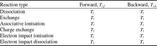
has different choices for different types of reactions, as shown in Table 1.
Control temperatures for different types of chemical reactions [Reference Casseau, Palharini, Scanlon and Brown28]

The reverse reaction rate coefficient can also be calculated from the equilibrium constant
 ${K_{eq,r}}$
and the forward reaction rate coefficient:
 \begin{equation}{k_{b,r}} = {k_{f,r}}/{K_{eq,r}}\end{equation}
2.3 Chemical reaction mechanism
Zhao [Reference Zhao48] constructed a H2-air reaction mechanism based on the air mechanism from Dunn and Kang [Reference Dunn and Kang18] and the H2-air mechanism from Jachimowski [Reference Jachimowski23]. The mechanism includes 12 species and 16 reactions, which can be divided into four categories: dissociation of O2 and N2 and the subsequent formation of NO, associative ionisation of N and O radicals, reaction of H2 with O2 and related radicals, and reaction of OH and N radicals. All reactions in the mechanism are listed in Table S1 of the supplementary material (SM). The thermodynamic parameters of all species adopt the NASA 9-parameter piecewise polynomial format, with data sourced from the Fluent standard database.
2.4 Turbulence model
The SST k-ω model [Reference Menter49] based on RANS method incorporates the transfer of turbulent shear stress in the definition of turbulent viscosity, making it suitable for various flows, including adverse pressure gradient flow, aerofoil and transonic shock waves. The model provides a reasonable balance between computational efficiency and accuracy in compressible flow.
The governing equations of the SST k-ω model are as follows:
 \begin{align}\frac{{\partial \left( {\rho k} \right)}}{{\partial t}} + \frac{{\partial \left( {\rho {u_j}k} \right)}}{{\partial {x_j}}} = \frac{\partial }{{\partial {x_j}}}\left[ {\left( {\mu + \frac{{{\mu_t}}}{{{\sigma_k}}}} \right)\frac{{\partial k}}{{\partial {x_j}}}} \right] + {P_k} - \rho {C_\mu }k\omega\end{align}
 \begin{align}\frac{{\partial \left( {\rho \omega } \right)}}{{\partial t}} + \frac{{\partial \left( {\rho {u_j}\omega } \right)}}{{\partial {x_j}}} = \frac{\partial }{{\partial {x_j}}}\left[ {\left( {\mu + \frac{{{\mu_t}}}{{{\sigma_\omega }}}} \right)\frac{{\partial \omega }}{{\partial {x_j}}}} \right] + {C_{\omega 1}}\frac{\omega }{k}{P_k} - {C_{\omega 2}}{\rho\omega^2} + 2\left( {1 - {F_1}} \right)\frac{\rho }{{\omega {\sigma_\omega }}}\frac{{\partial k}}{{\partial {x_j}}}\frac{{\partial \omega }}{{\partial {x_j}}}\end{align}
where
 $k$
is the turbulent kinetic energy,
 $\mu $
is the dynamic viscosity,
 ${\mu_t}$
is the turbulent viscosity,
 ${P_k}$
is the generation term of the turbulent kinetic energy,
 $\omega $
is the specific dissipation rate,
 ${\sigma_k}$
and
 ${\sigma_\omega }$
are the turbulent Prandtl numbers for
 $k$
and
 $\omega $
, respectively.
 ${C_\mu }$
,
 ${C_{\omega 1}}$
,
 ${C_{\omega 2}}$
are the model parameters,
 ${F_1}$
is a blending function. The turbulent viscosity is calculated as follows:
 \begin{equation}{\mu_t} = \frac{{\rho k}}{{\max \left[ {\omega ,\frac{{S{F_2}}}{{{a_1}}}} \right]}}\end{equation}
where
 ${F_2}$
is the blending function,
 ${a_1}$
is the model parameters and
 $S$
is the shear stress. Default values are selected for all model parameters.
2.5 Turbulence-chemistry interactions
The partially stirred reactor (PaSR) model [Reference Chomiak and Karlsson50, Reference Golovitchev, Nordin, Jarnicki and Chomiak51] is suitable for supersonic combustion [Reference Li, Wang and Li40, Reference Wu, Piao, Xie and Ren52]. This model assumes that a cell in mesh can be divided into reacting zone and non-reacting zone. The reacting volume fraction
 $\kappa $
and the time scale
 ${\tau^*}$
are expressed as follows:
 \begin{align}\kappa = \frac{{{t_c}}}{{{t_c} + {t_{mix}}}}\end{align}
 \begin{align}\tau^{*} = Min\left({t_c},{t_{mix}}\right)\end{align}
where
 ${t_c}$
,
 $\;{t_{mix}}$
are the chemistry time scale and the mixing time scale, expressed as:
 \begin{align}{t_c} = max\left(\frac{\rho {Y_\alpha }}{\omega_\alpha}\right)\end{align}
 \begin{align}{t_{mix}} = {C_{mix}}\left( {\frac{k}{\varepsilon }} \right)\end{align}
where
 ${\omega_\alpha }$
is the reaction rates of species
 $\;\alpha $
,
 ${C_{mix}}$
is model constant,
 $\;k$
is the turbulent kinetic energy and
 $\varepsilon $
is the turbulent kinetic energy dissipation rate. The source term of the species mass conservation equation is expressed as:
 \begin{equation}{S_\alpha } = \frac{{\rho \kappa }}{{{\tau^*}}}\left( {Y_\alpha^* - {Y_\alpha }} \right)\end{equation}
where
 $_\alpha^*$
is the mass fraction of species
 $\alpha $
in the reacting zone.
3.0 Compute configuration and simulation settings
The 3D DLR scramjet combustor, depicted in Fig. 1(a), is utilised in the simulation. Several streamwise locations where experimental data were measured are marked on the figure. The combustor has a total length of 400 mm, comprising a 100 mm straight section and a 300 mm single-sided expansion section. The inlet, measuring 45 × 50 mm, is connected to a Mach 2 Laval nozzle. A fuel strut, angled at 12 degrees, is positioned 77 mm from the inlet, with 15 1 mm injectors located at the centre of the strut’s bottom for fuel injection. When dividing the grid, only one injector is considered, and the combustor width is shortened to 3 mm. This simplification method may overestimate the mixing uniformity near the injector and underestimate the local concentration gradient. The possible common circulation zone formed among multiple injectors is ignored. But overall, the impact is ignorable [Reference Wu, Zhang, Yao and Fan53]. Grid independence verification has been conducted, with results presented in Fig. S1 of the supplementary material. Ultimately, a hexahedral grid with 1,110,675 cells is employed to discretise the computational domain, as shown in Fig. 1(b).
Schematic diagram of the DLR combustor (a) and mesh adopted to discrete the computational domain (b).

Two conditions are selected for simulation, the inflow Mach are 2 and 6, and the corresponding flight Mach are 3 and 9.8, respectively. The two working conditions correspond respectively to supersonic combustion and hypersonic combustion. The inlet and injector are set as pressure inlet, and their specific variables are shown in Table 2. The turbulence intensity is calculated by
 $I = 0.16 \times R{e^{ - 0.125}}$
and
 $R$
is the hydraulic diameter. The upper and lower walls and strut are set as non-slip adiabatic walls. The left and right walls are set as periodic boundary.
Boundary conditions of combustor inlet and injector

The simulation is conducted using Ansys Fluent with a two-temperature density-based solver, and the implicit Coupled Algorithm is selected as the solution method. For all control equations, the convective flux is discretised using the Advection Upstream Splitting Method (AUSM) scheme, and the gradient is discretised using the Green-Gauss Node Based method. The flow, turbulent kinetic energy, specific dissipation rate, translational temperature, and vibrational temperature are discretised using the second-order upwind scheme. During the solution, solution steering is enabled, the supersonic flow type is chosen. Full multigrid (FMG) initialisation is used to obtain a better initial solution, thereby accelerating the convergence rate.
4.0 Results and discussions
The present work first carries out numerical simulation with inflow Mach 2, the corresponding results of the non-reactive flow and the reactive flow are given in sections 4.1 and 4.2, including the thermochemical non-equilibrium analysis as presented in Figs 11, 12, 13 and 14. To explore the thermochemical non-equilibrium effect under higher Mach conditions, the present work simulates the inflow Mach 6 condition, and the results are given in Figs 15, 16, 17, 18 and 19. Furthermore, to investigate the influence of thermochemical non-equilibrium on the performance of combustor, equilibrium simulations of the two inflow conditions are also calculated, and the comparison results are illustrated in Figs 14 and 19.
4.1 Non-reactive flow field under inflow Mach 2 condition
Figure 2 presents the comparison of numerical and experimental schlieren images of the combustor. The supersonic airflow enters the combustor, generating extremely weak incident shock waves on the upper and lower walls, whose influence is negligible. At the strut’s leading edge, the airflow generates oblique shock waves, which undergo multiple reflections and deflections upon interacting with the walls and the H2 jet. Due to the unilateral expansion structure of the combustor, the reflected shock waves on the upper walls hit the H2 jet at a farther position, forming an asymmetric flow field. Concurrently, expansion waves and shock waves are successively generated at the rear end of the strut. In the experiment, several fine shock waves are generated within the range of x = 110 – 180 mm. This is caused by the rough walls of the combustor and the strut trailing edge, which could not be captured in the simulation. The resulting shock waves merge with the reflected shock wave on the lower wall at x = 175 mm forming a stronger shock wave. As the flow continues downstream, the shock wave intensity progressively weakens, and the changes in the flow field parameters gradually diminish. Overall, the results of the non-reactive non-equilibrium simulation are consistent with the experimental data.
The comparison between the experimental schlieren image (a) [Reference Genin and Menon41] and numerical schlieren images (b).

Figure 3 displays the pressure distributions along the lower wall and the centreline (y = 25 mm) of the combustor, comparing these results with the experimental data. The simulation and experimental results are generally consistent when accounting for vibrational non-equilibrium. However, the pressure peak predicted by the simulation is lower than that observed experimentally.
The comparison of the experimental pressure profiles and the numerical results along the lower wall (a) and centreline (b) of the combustor.

The centreline intersects three reflected shock waves at x = 150, 240, and 325 mm, where the pressure initially rises and then falls, creating three distinct peaks. The first shock wave reflection on the lower wall at x = 110 mm causes an increase in pressure, while the expansion wave generated by the strut at x = 130 mm leads to a pressure decrease. Subsequently, continuous shock wave reflections occur between x = 150 and 400 mm, with each reflection generating a pressure peak that gradually diminishes.
Figure 4 illustrates the distributions of streamwise velocity at four different positions within the combustor, comparing these results with experimental values. Figure 5 shows the contour of the streamwise velocity on the central plane. While the general trends of the simulation result are consistent with the experimental values, discrepancies in velocity values are observed at certain locations. H2 is injected at approximately 1,200 m/s and accelerates to 1,600 m/s over a very short distance. Due to the low pressure behind the strut, the velocity is deflected, most of the H2 decelerates to 200 m/s and flows downstream. But as the combustor expands, the velocity gradually increases within the 100–200 mm range, ultimately stabilising at 700 m/s.
Distributions of streamwise velocity at streamwise locations of x = 118 mm (a), x = 165 mm (b), x = 197 mm (c), x = 273 mm (d).

Contour of streamwise velocity on the central plane.

Figure 6 shows the streamwise velocity fluctuation distributions in two different streamwise locations within the combustor, calculated using
 $v' = {\left( {2k/3} \right)^{0.5}}$
. The results are similar to the previous results of DLR simulation using flamelet modeling [Reference Oevermann39]. The simulation captures the expected variation trend, but the peak of velocity fluctuation is larger than the experimental value.
Distributions of streamwise velocity fluctuation at streamwise locations of x = 222 mm (a), x = 247 mm (b).

The above analysis indicates that considering the vibrational non-equilibrium effect in the cold state simulation of the DLR combustor yields comparatively accurate results. Although there are some differences from the experimental data, the trends are similar to DLR simulations in our previous work using multiple mechanisms [Reference Li, Wang and Li40] and using LES [Reference Genin and Menon41]. The vibrational non-equilibrium effect is weak in present non-reactive flow field. Specific analysis of the vibrational non-equilibrium effect in the reactive flow field is presented in the following section.
4.2 Reactive flow field under inflow Mach 2 condition
Figure 7 provides the comparison between experimental and numerical schlieren images. The numerical simulation results display a reasonable overall shock wave structure. Compared with the non-reactive flow field, the most significant difference is that the H2 jet behind the strut becomes wider due to the reaction and the expansion waves become more obvious. After the shock waves and expansion waves reflect off the walls, their intensity diminishes, making it difficult for them to pass through the jet and causing them to almost disappear. Consequently, there are no reflected shock waves after the position of x = 200 mm. The experimental measurement indicates that the reaction zone initially expands and then contracts immediately, whereas the simulation shows smaller contraction of the reaction zone during downstream development. H2 is injected into the combustor at Mach 1. Similarly, the velocity in the x-direction is reduced due to deflection at low pressure. After accelerating due to combustion heat release, the velocity increases back to Mach 1 at x = 250 mm, indicating that the reaction zone is overall subsonic.
The comparison of experimental schlieren image (a) [Reference Genin and Menon41] and numerical schlieren images (b).

Figure 8(a) illustrates the simulated streamwise velocity at the geometric centreline against experimentally measured data. Due to the low pressure behind the strut, strong deflection and deceleration occur. The jet then accelerates, fluctuates slightly near the shock wave, and stabilises downstream. The experiment data follow a similar trend to the simulation, but the minimum value is larger, and the increasing trend is slightly faster. Figure 8(b), (c) and (d) illustrate the streamwise velocity distributions at three locations. Owing to the penetration depth of the jet is underestimated in the simulation, the centre at x = 118 mm is in the deflection zone, resulting in inwardly concave single-peak. The results in the mainstream zone on both sides of the centre are consistent with the experiment. Due to the acceleration caused by combustion heat release expansion and the subsonic jet contraction in the midstream, the velocity at x = 165 mm is overestimated. At x = 247 mm, the centre has been accelerated beyond that of the mainstream zone.
Distributions of streamwise velocity at the geometric centreline (a) and the streamwise locations of x = 118 mm (b), x = 165 mm (c), x = 247 mm (d).

Figure 9 compares the simulated streamwise velocity fluctuation at three streamwise locations with the experimental data. The results indicate that the simulation is generally in agreement with the experiment. The streamwise velocity fluctuation of the jet more closely with the experimental data than that of the mainstream zone.
Distributions of streamwise velocity fluctuation at streamwise locations of x = 118 mm (a), x = 165 mm (b), x = 197 mm (c).

As shown in Fig. 10, the temperature distributions obtained from the simulation at three streamwise positions is compared with the experimental data. At x = 118 mm, the simulation captures the inwardly concave single-peak at the centre, but the combustion zone is narrow. Intense combustion occurs at x = 165 mm, as shown in Fig. 7, the simulated jet doesn’t contract in time, resulting in a larger width. At x = 273 mm, located in the mid downstream region of the combustor, the simulation results are generally consistent with the experiment, although the temperature peak is slightly higher. This indicates that the simulation slightly overestimates the combustion heat release in the reaction zone. However, the overall trend of the flow field is consistent with the experiment, similar to the results in our previous work [Reference Li, Wang and Li40] and the DLR simulation using LES by Genin et al. [Reference Genin and Menon41]. The result of the flow field considering the non-equilibrium effect is close to the equilibrium flow field.
Distributions of translational temperature at streamwise locations of x = 118 mm (a), x = 165 mm (b), x = 273 mm (c).

The translational-vibrational non-equilibrium effect is assessed by analysing the translational-vibrational relaxation time and temperature distributions. Figure 11 illustrates contours of mass-averaged translational-vibrational relaxation time and path-lines coloured by flow time. The flow time in the circulation zone at the front of the combustion zone and the downstream of the mainstream is relatively long, but the flow time in other areas is very short. According to the Millikan and White formula, the translational-vibrational relaxation time of the same species is negatively correlated with temperature. Thus, the relaxation times of different regions are arranged from small to large as combustion zone, shear layer, boundary layer and mainstream.
Contours of mass-averaged translational-vibrational relaxation time (a), path-lines coloured by flow time (b) on the central plane.

Define the vibrational relaxation Damköhler number
 ${D_a}_{vib}$
, expressed as the ratio of the flow time to the vibrational relaxation time:
 \begin{equation*}{D_a}_{vib} = {\tau_{flow}}/{\tau_{vib}}\end{equation*}
If
 ${D_a}_{vib}$
< 1, it indicates that the vibrational non-equilibrium effect in the flow is significant.
 ${D_a}_{vib}\geq1$
, it indicates that the flow can achieve translational-vibrational relaxation.
Figure 12(a), (b) and (c) presents the distributions of the translational temperature, vibrational temperature, and their difference in the combustor, respectively. Since the inflow is in vibrational equilibrium, the translational and vibrational temperatures of the mainstream are equal before the shock waves. When passing through the shock wave, kinetic energy of inflow is converted to internal energy, which includes translational energy and vibrational energy. The translational temperature of mainstream increases and the relaxation time is 0.25–0.3 s,
 ${D_a}_{vib}$
is less than 1. Thus, the translational and vibrational energy do not have enough time to convert, resulting in non-equilibrium. As H2 is injected into the combustor, the vibrational temperature rises within a very short distance, while the translational temperature remains unchanged, this phenomenon is similar to the high vibrational temperature near the injector of Hyshot II simulation under thermal non-equilibrium conditions [Reference Fiévet, Voelkel, Koo, Raman and Varghese35]. This may be due to the smaller injector, which increases the collision frequency and causes the vibrational excitation. The jet deflects to both sides, this zone has
 ${D_a}_{vib}$
much less than 1, and it is in a vibrational cooling state.
Contours of translational temperature (a), vibrational temperature (b) and the difference between them (c) on the central plane.

Combustion heat release converts chemical energy into internal energy and the relaxation time of the combustion zone is 10–6 s, which is less than flow time 2 × 10⁻³ s.
 ${D_a}_{vib}$
is greater than 1. Therefore, translational and vibrational energy can be rapidly converted to reach thermal equilibrium. As the jet develops downstream and leaves the combustion zone, internal energy is converted into kinetic energy. The temperature decreases overall, but the translational temperature decreases even more. The relaxation time is slightly lower than the flow time,
 $\;{D_a}_{vib}$
is approximately equal to 1, so the downstream jet core is in a weaker vibration cooling state. The relaxation time of the shear layer and boundary layer are both above 1 ms, leading to non-equilibrium.
In summary, it is evident that the translational-vibrational non-equilibrium effect stems from two primary factors. When kinetic energy and chemical energy are converted into internal energy, there is a significant difference in the degree of conversion to translational and vibrational energy. In the region where the translational-vibrational relaxation time is larger than the flow time, that is,
 ${D_a}_{vib}$
is less than 1, the translational energy and vibrational energy cannot be quickly converted into each other to make the translational temperature equal to the vibration temperature, resulting in the translational-vibrational non-equilibrium effects.
Figure 13 presents the mass fraction contours of H2 and NO in the combustor. H2 is injected into the combustor and immediately undergoes intense combustion upon contact with O2 (
 ${\rm{O}} + {\rm{H}} + {\rm{M}} \to {\rm{HO}} + {\rm{M}}$
,
 ${\rm{OH}} + {\rm{H}} + {\rm{M}} \to {{\rm{H}}_2}{\rm{O}} + {\rm{M}}$
), creating a high-temperature zone that causes N2 to dissociate (
 ${{\rm{N}}_2} + {\rm{M}} \to 2{\rm{N}} + {\rm{M}}$
). N radicals formed by N2 dissociation combine with O radicals forming NO and reacts with OH forming NO and H (
 ${\rm{N}} + {\rm{OH}} \to {\rm{H}} + {\rm{NO}}$
,
 ${\rm{N}} + {\rm{O}} + {\rm{M}} \to {\rm{NO}} + {\rm{M}}$
), their mass fraction contours are shown in Fig. S2 of SM. At the core of the jet, x = 150–200 mm, the peak mass fraction of NO is 5.68 × 10⁻⁶. The mass fraction of leaving the combustion zone has decreased to 1.7 × 10⁻⁶. Due to the highest temperature in the combustion zone being only 2,200 K and the activation temperature for N2 dissociation reaction being too high, the rate of the reaction is relatively low. Thus, the dissociation of N2 and subsequent reactions is weak in lower Mach combustion.
Mass fraction contours of H2 (a) and NO (b) on the central plane.

To evaluate the influence of thermochemical non-equilibrium from a macroscopic perspective, combustion efficiency and net thrust, as important parameters for evaluating combustion performance of combustor, are calculated by following formulas:
 \begin{align}\eta = \frac{{\left[ {\int\!\!\!\int \rho u{Y_{{H_2}O}}dydz/{M_{{H_2}O}}} \right]_{inlet}^x}}{{{{\dot m}_{{H_2}}}/{M_{{H_2}}}}}\end{align}
 \begin{align}F = \left[ {\int\!\!\!\int \left( {\rho uu + p} \right)dydz} \right]_{inlet}^x\end{align}
where ∫∫ represents the surface integral of the
 $yz$
plane perpendicular to the
 $x$
axis.
 $\rho $
,
 $p$
,
 $u$
,
 ${Y_{{H_2}O}}$
are the density, pressure, velocity in the
 $x$
direction and mass fraction of H2O of the different grid cells in the plane, respectively.
 ${\dot m_{{H_2}}}$
is the mass flow rate at the injector.
 ${M_{{H_2}O}}$
and
 ${M_{{H_2}}}$
are the molecular weight of H2O and H2.
Figure 14(a) and (b), comparing the vibrational equilibrium and non-equilibrium, presents the combustion efficiency and net thrust at different streamwise locations in the combustor. The combustion efficiency in the midstream of the combustor is close in both states, while the non-equilibrium combustion efficiency in the upstream and downstream of the combustor is slightly higher. The non-equilibrium combustion efficiency at x = 120 mm is 8.38%, which is relatively 10% higher than the equilibrium combustion efficiency. The non-equilibrium combustion efficiency at outlet is 95.4%, relatively 0.37% higher than that in equilibrium. Since only 1/15 of the combustor is calculated, the net thrust is at a low level overall. The net thrust in non-equilibrium is always higher than that in equilibrium. The non-equilibrium net thrust at x = 160 mm is 0.26 N, which is higher than the equilibrium net thrust 52.94% relatively. The non-equilibrium net thrust at the outlet is 3.72 N and higher than the equilibrium 0.27% relatively. High vibrational temperature promotes the dissociation of H2 (
 ${{\rm{H}}_2} + {\rm{M}} \to {\rm{H}} + {\rm{H}} + {\rm{M}}$
) near the strut. Most of the O, H radicals react by
 ${\rm{O}} + {\rm{H}} + {\rm{M}} \to {\rm{HO}} + {\rm{M}}$
and
 ${\rm{OH}} + {\rm{H}} + {\rm{M}} \to {{\rm{H}}_2}{\rm{O}} + {\rm{M}}$
. Compared with the equilibrium, more H2O is produced in the non-equilibrium, which means higher combustion efficiency. The improvement of combustion efficiency near the strut indicates that the flame has higher stability in the initial stage of combustion, as in Fig. S5 of SM. Overall, the translational-vibrational non-equilibrium slightly promotes combustion and enhances the performance of the scramjet. To further improve the combustion performance, add one fuel injector on each side wall of the strut, and allocate 5–10% of the H2 flow rate from the original fuel injector to these two fuel injectors. In this way, the local equivalent ratio near the strut walls can be increased, enabling more O radicals to react with H radicals.
Distributions of combustion efficiency (a) and net thrust (b) at different streamwise locations.

4.3 Non-reactive flow field under inflow Mach 6 condition
Figure 15 illustrates the Mach number contour of the non-reactive flow. The hypersonic turbulent boundary layer separates at the combustor inlet, resulting in two long incident shock waves. They develop downstream and merge with the oblique shock wave in front of the strut, forming stronger shock waves. Simultaneously, a subtle expansion wave is generated at the bottom of the strut, leading to a recovery of the Mach number. The merged shock waves are reflected by the upper and lower walls and impact the H2 jet. But the shock angle is small, so the shock waves only reflect twice before leaving the combustor. Due to the unilateral expansion of the combustor, the upper shock wave impacts the jet further downstream than the lower shock wave. The shock wave intensity decreases after passing through the jet. Following H2 injection, a shear layer is formed between the jet and the mainstream due to the significant velocity difference. A droplet-like high Mach area forms after the H2 injection, which is wrapped by a low-speed zone. The boundary layer separates at the walls of the combustor, forming a circulation zone at the junction between the shock waves and walls.
Contour of Mach number on the central plane.

4.4 Reactive flow field under inflow Mach 6 condition
Figure 16 illustrates the Mach number and streamwise velocity contours of the reacting flow. The shock wave structure and the degree of boundary layer separation are essentially consistent with those in the non-reacting flow, with the primary difference being the extent of the low-speed area of the jet. Since the combustion of H2 occurs at the junction of the jet and the mainstream, the heat release from combustion causes the temperature to rise, which in turn increases the local sound speed. Given that the velocity remains largely unchanged, the Mach number decreases correspondingly. As the jet develops downstream, the combustion zone gradually extends to the upper and lower walls, while the combustion itself remains at the supersonic level.
Contours of Mach number (a), streamwise velocity (b) on the central plane.

Figure 17(a), (b) and (c) presents the contours of translational temperature, vibrational temperature, and their difference in the combustor, respectively. Compared to combustion under Mach 2 condition, the flow with Mach 6 leads to significant changes in shock wave structure, with the combustion zone shifting from the jet core to the shear layer and generating excessively high temperatures on the walls. Therefore, the non-equilibrium effect is also significantly different from Mach 2 combustion. Due to the prolonged and increased intensity of the incident shock waves, the translational and vibrational temperatures of the inflow generate a temperature difference of 30–70 K when passing through the incident shock waves. When the inflow passes through the inclined shock wave in front of the strut, the temperature difference increases to over 200 K, and the non-equilibrium effect strengthens progressively. The non-equilibrium is strongest on the walls, where the translational temperature is above 1,000 K higher than the vibration temperature, and higher than 2,000 K at x < 95 mm. The non-equilibrium effect becomes stronger with multiple passes of shock waves. Similar to Mach 2 flow, when H2 gas is injected, the vibrational mode is excited, and the translational temperature remains constant. However, due to combustion occurring in the shear layer under inflow Mach 6 condition, the interior of the jet always maintains a state where the vibrational temperature is higher than the translational temperature. The combustion zone is in vibrational equilibrium, and the non-equilibrium effect outside the combustion zone is significant.
Contours of translational temperature (a), vibrational temperature (b) and the difference between them (c) on the central plane.

The simulation results of the inflow Mach 3.3 are shown in Figs S8 and S9. According to results of Mach 2, 3.3 and 6, the non-equilibrium zones at the walls become more obvious as the inflow Mach number increases. The generation of the mainstream non-equilibrium zone is related to the shock wave structure. The structure of the combustion zone is closer to the shear layer combustion. If there is no stable jet flame, there will be no large-scale equilibrium zone in the jet.
According to Fig. 18, after fuel is injected, the mass fraction of H2 remains high within the jet for a considerable distance, with a significant concentration gradient only in the shear layer. A small amount of OH radicals and a substantial amount of H2O are produced (
 ${\rm{O}} + {\rm{H}} + {\rm{M}} \to {\rm{HO}}$
,
 ${\rm{OH}} + {\rm{H}} + {\rm{M}} \to {{\rm{H}}_2}{\rm{O}} + {\rm{M}}$
). Further downstream, near the outlet, the jet mixes with the mainstream, accelerating the consumption of H2, which significantly reduces its mass fraction and produces more H2O. Due to the high inflow Mach, the inflow stagnates on the walls, resulting in a temperature higher than the combustion temperature. Therefore, the dissociation of N2 (
 ${{\rm{N}}_2} + {\rm{M}} \to 2{\rm{N}} + {\rm{M}}$
) and the generation of NO (
 ${\rm{N}} + {\rm{OH}} \to {\rm{H}} + {\rm{NO}}$
,
 ${\rm{N}} + {\rm{O}} + {\rm{M}} \to {\rm{NO}} + {\rm{M}}$
) mainly occur at the walls. Since H2 does not flow towards the upper and lower walls, the O and H reactions (
 ${\rm{O}} + {\rm{H}} + {\rm{M}} \to {\rm{HO}} + {\rm{M}}$
,
 ${\rm{OH}} + {\rm{H}} + {\rm{M}} \to {{\rm{H}}_2}{\rm{O}} + {\rm{M}}$
) do not occur here and have no direct impact on the combustion process. The mass fraction of NO near the walls is always higher than 0.09. The maximum value reaches 0.11 at x = 150 mm. Simultaneously trace amounts of e- and NO+ are produced (
 ${\rm{N}} + {\rm{O}} \to {{\rm{e}}^- } + {\rm{N}}{{\rm{O}}^+ }$
). The dissociation of N2 also occurs in the shear layer, producing trace amounts of NO, OH, O and N radicals, etc. The mass fraction of NO in the front end of the combustion zone is 0.03 as shown in Fig. S3 and Fig. S4 of SM.
Mass fraction contours of H2 (a) and NO (b) on the central plane.

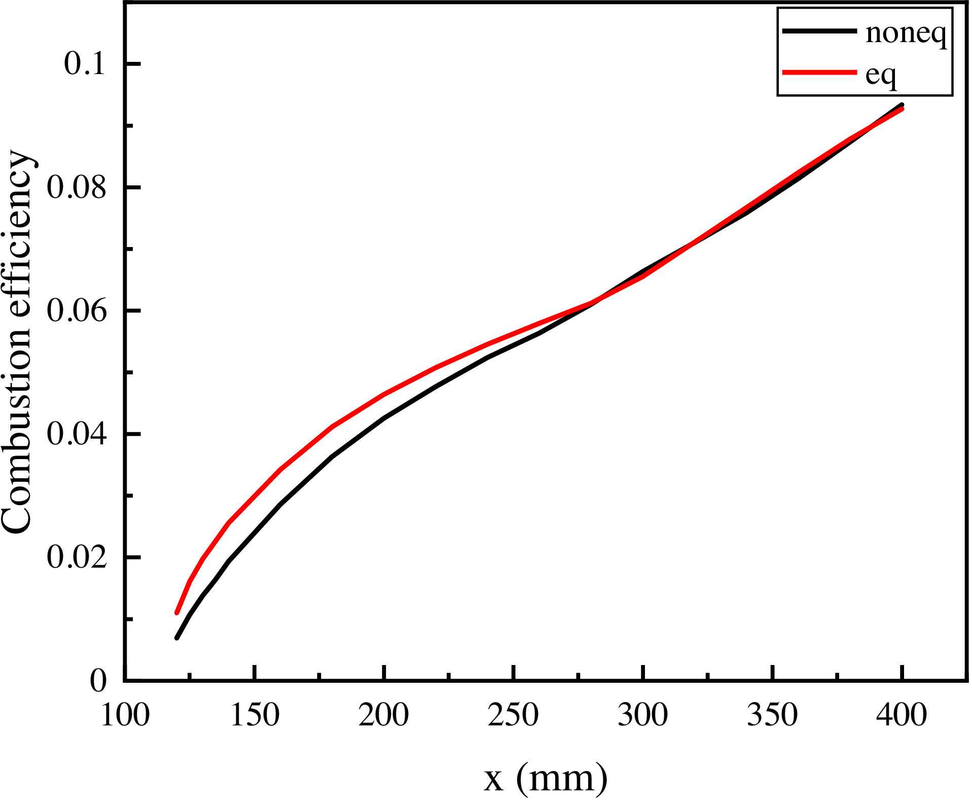
Based on the simulation results of thermochemical equilibrium and non-equilibrium with Mach 6 condition, Fig. 19 compares their combustion efficiency. Before x = 280 mm, the equilibrium combustion efficiency is higher than that of non-equilibrium. The high temperature of the strut walls promotes the generation of N and O radicals. Compared to equilibrium, higher vibrational temperatures promote the dissociation of H2 (
 ${{\rm{H}}_2} + {\rm{M}} \to 2{\rm{H}} + {\rm{M}})$
. The O radicals are more likely to react with N radicals to generate more NO, which competes with the reaction between H and O (
 ${\rm{O}} + {\rm{H}} + {\rm{M}} \to {\rm{HO}} + {\rm{M}}$
,
 ${\rm{OH}} + {\rm{H}} + {\rm{M}} \to {{\rm{H}}_2}{\rm{O}} + {\rm{M}}$
). Therefore, the production of NO means a decrease in combustion efficiency (as shown in Fig. S6 and Fig. S7 of SM). After x = 280 mm, the two curves are very close and rise alternately. The non-equilibrium combustion efficiency at outlet is 9.34%, which is 0.75% higher than the equilibrium combustion efficiency, relatively. This is because under the condition of Mach 6, no flow circulation zone is formed in the combustor to improve the combustion efficiency, and the combustion only occurs in the form of shear layer flames.
The combustion efficiencies of thermochemical equilibrium and non-equilibrium under Mach 6 conditions along the streamwise locations.

Compared to combustion under Mach 2 condition, combustion efficiencies are significantly reduced, with a reduction value of 86% at the outlet. As a possible prediction, the thermochemical non-equilibrium effect on combustion performance is more complex and significant under high Mach condition. It inhibits the initial upstream combustion and slightly promotes downstream combustion under inflow Mach 6 condition. To improve the combustion performance, additional injectors can be set on the strut walls and the upper and lower walls, or cavities can be added at appropriate positions on the upper and lower walls. The function of these methods is to increase the local equivalent ratio and flow time, enabling more O radicals to react with H radicals, thereby enhancing the combustion efficiency while inhibiting the generation of NO. In addition, by adding a bluff-body at an appropriate position in the combustor. A stable circulation zone will be formed behind the bluff-body, prolonging the flow time and promoting the thorough mixing of fuel and air [Reference Zhang, Zhao, Shi, Huang, Zhang and Sun54].
5.0 Conclusion
The present work investigates the thermochemical non-equilibrium effect in the DLR combustor using a two-temperature model combined with a vibration-chemistry coupling model. Two operating conditions with inflow Mach 2 and 6 are selected for study. The simulation results illustrate that the vibrational non-equilibrium effect depends on energy conversion behaviour and vibrational relaxation time. When kinetic energy and chemical energy are converted into internal energy, there is a significant difference in the degree of conversion to translational and vibrational energy. If the translational-vibrational relaxation time is larger than the flow time, such as the relaxation time of the mainstream after shock wave is 0.25 s for the condition of inflow Mach 2, and the flow time is 3 × 10⁻⁵ s, non-equilibrium will occur. The combustion zone reaches equilibrium because of the relaxation time of the combustion zone is 10−6 s, which is less than flow time 2 × 10⁻³ s.
For the condition with inflow Mach 2, due to the highest temperature in the combustion zone being only 2,200 K and the activation temperature for N2 dissociation reaction being too high, the rate of the reaction is relatively low. The maximum value of mass fraction of NO is only 5.68 × 10⁻⁶ in the flow field. Significant differences exist between the flow fields with Mach 2 and 6. A clear boundary layer separation at Mach 6. Its combustion occurs at the shear layer, which is in translational-vibrational equilibrium, and there are varying degrees of non-equilibrium in other locations. When the inflow passes through the oblique shock wave, the translational temperature is 200 K higher than the vibrational temperature. The temperature difference on the walls is always higher than 1,000 K. Dissociation of N2 and production of NO mainly occurs on the strut walls and the upper and lower walls of the combustor at Mach 6 and the maximum value of mass fraction of NO is 0.11.
The thermochemical non-equilibrium slightly promotes combustion at Mach 2 with a relative increase of 10% in combustion efficiency near the injector and a relative increase of 0.37% at the outlet. Adding additional injectors appropriately on the strut walls and changing the distribution of the fuel flow rate is conducive to improving the combustion efficiency. The influence of non-equilibrium on combustion efficiency is more complex at Mach 6. Non-equilibrium effect inhibits the initial upstream combustion and slightly promotes downstream combustion. Additional injectors can be set on the strut walls and the upper and lower walls, or cavities can also be added at appropriate positions on the upper and lower walls. This increases the local equivalent ratio, enabling more O radicals to participate in the combustion reaction, thereby enhancing the combustion efficiency while inhibiting the generation of NO.
Acknowledgements
This work is supported by the TaiHang Laboratory (No. A2043). Thanks to the National Supercomputing Chengdu Centre for providing the computing resources.
Supplementary material
To view supplementary material for this article, please visit https://doi.org/10.1017/aer.2025.10070