




1 Introduction
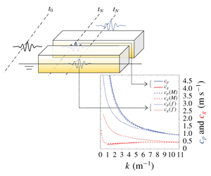
In side-by-side scenarios, one vessel may be moored alongside another, creating a gap that is very narrow relative to the principal dimensions of the two bodies. One practical application might be an offloading operation between a floating liquefied natural gas facility and a liquified natural gas carrier (Zhao et al. Reference Zhao, Milne, Efthymiou, Wolgamot, Draper, Taylor and Eatock Taylor2018). The fluid inside the narrow gap may experience significant resonant response (gap resonance) when excited at particular wave frequencies.
Early pioneering studies (Molin Reference Molin2001; Molin et al. Reference Molin, Remy, Kimmoun and Stassen2002; Sun, Eatock Taylor & Taylor Reference Sun, Eatock Taylor and Taylor2010) have demonstrated that gap resonances are standing waves in a gap, where the gap length is close to an integer number of half-wavelengths for each standing wave (or gap mode). The gap resonances with different but close mode frequencies interfere in the gap, making the resonance rather complex. Gap resonance is an interesting hydrodynamic phenomenon, also in the sense that the narrow width makes it difficult for wave energy to ‘escape’ from the gap, leading to large responses at resonance. In such a scenario, viscous damping becomes relatively important as the radiation damping is small.
Various methods have been proposed in the frequency domain to consider the viscous damping contribution to obtain reasonable agreement between potential flow calculations and physical model test results in gap resonance. For instance, Huijsmans, Pinkster & De Wilde (Reference Huijsmans, Pinkster and De Wilde2001) suppressed vertical motion in the gap completely by introducing a rigid lid, Newman (Reference Newman and Kashiwagi2001) split the gap motion into generalized modes, allowing different damping rates for each motion and Chen (Reference Chen2005) introduced a dissipative damping term in the free-surface condition.
In addition to frequency-domain analysis, intensive time-domain simulations can be conducted to account for viscous and nonlinear contributions. For instance, Kristiansen & Faltinsen (Reference Kristiansen and Faltinsen2008) ran a fully nonlinear two-dimensional numerical wavetank coupled with an inviscid vortex tracking method, suggesting that flow separation is the main source of discrepancy between linear potential theory and model tests. A model is then developed for the estimation of viscous damping, based on small-amplitude harmonic flows through a slot in a slatted screen (Faltinsen & Timokha Reference Faltinsen and Timokha2015). Feng & Bai (Reference Feng and Bai2015) carried out fully nonlinear numerical simulations and reported that nonlinearity may slightly increase the resonant frequency, although with limited effect on the amplitude. Using a multi-phase Navier–Stokes equation model, the flow field in the gap is examined in Feng et al. (Reference Feng, Bai, Chen, Qian and Ma2017) with a focus on vorticity.
Numerous studies have been made to improve the agreement between numerical simulations and experimental data, by better understanding and modelling the damping. It seems that the majority of the efforts have been focusing on the resonant elevations at an individual location (e.g. the centre of a gap), while very few have considered the spatio-temporal structure of enhanced surface elevation along the gap. How wave groups propagate along the gap and how these couple into the gap resonant modes have not been studied previously.
In light of the above, we carried out a series of experiments (using the same set-up as in Zhao et al. (Reference Zhao, Wolgamot, Taylor and Eatock Taylor2017)) to investigate the group dynamics and wave propagation of the resonant responses in a narrow gap. The gap resonance is excited by focused transient wave groups from different headings. A brief description of the experimental set-up follows in § 2. The gap resonance phenomenon driven through a linear process is discussed in detail in § 3. The evolution of the gap resonance is briefly discussed, and the linear transfer functions, with multiple peaks corresponding to various gap modes, are reported in § 3.2. The temporal and spatial structure of the gap resonance is demonstrated more clearly in § 4 through nonlinear excitation – a frequency-doubling process. Some new observations on the phase speed and group velocity of components related to the gap resonance modes are given in § 5. We show that the group velocity within the gap drops to one twentieth of the phase speed close to the lowest gap mode, significantly different to that for deep-water free waves. Finally, some conclusions are drawn at the end of this study.
2 Experimental set-up
Experimental set-up: (a) sketch (not to scale) of the fixed boxes in different heading excitations, with the red symbols showing the locations of the wave probes; (b) a snapshot of the fixed box hull (yellow) rigidly connected to the gantry (blue) in the wave basin. The end of the narrow gap is marked by two vertical green lines.

The experiments were conducted in the Deepwater Wave Basin at Shanghai Jiao Tong University. The basin is 50 m long, 40 m wide and the water depth was set to 10 m. To focus on the gap responses and to simplify the study, we selected two identical rectangular boxes to represent a side-by-side moored two-body system. Each model is 3.333 m long, 0.425 m high, 0.767 m wide and the gap width between them is 0.067 m. The vessel models have round corners at both bilges, each with a radius of 0.083 m running along the full length, as shown in figure 1.
During the model tests, the two boxes are fixed to a gantry which provided enough stiffness to hold them rigidly in place. Each box was immersed to a draft of 0.185 m. As shown in figure 1, there are seven wave gauges (WG) 1 and 7, 2 and 6, 3 and 5 being symmetric in pairs about the gap centre, and WG4 being central in the gap. A more detailed description was reported in a previous study (Zhao et al. Reference Zhao, Wolgamot, Taylor and Eatock Taylor2017).
Rather than generating random waves in the tank, requiring long duration runs, we used transient focused wave groups as the incident waves. Prior to the experiments, a series of transient wave groups were generated in the absence of the model, based on a hypothetical Gaussian spectrum (representative of swells) given by
 $$\begin{eqnarray}S_{\unicode[STIX]{x1D702}}(f)=\frac{H_{s}^{2}}{16}\frac{1}{\unicode[STIX]{x1D6FF}\sqrt{2\unicode[STIX]{x03C0}}}\exp \left[-\frac{(f-f_{p})^{2}}{2\unicode[STIX]{x1D6FF}^{2}}\right],\end{eqnarray}$$
where  $H_{s}$ refers to an assumed significant wave height,
 $f_{p}$ the peak frequency of the spectrum and
 $\unicode[STIX]{x1D6FF}=0.0775~\text{Hz}$.
Two sets of transient wave groups were generated (see details in appendix A): one of them has a spectral peak frequency  $f_{p}=f_{m=1}=1.02~\text{Hz}$ (where
 $f_{m=1}$ is the frequency of the mode with one half-wavelength along the gap in this experiment) and the other
 $f_{p}={\textstyle \frac{1}{2}}\,f_{m=1}$. The two wave group tests drive the gap resonance through different processes – the former (
 $f_{p}=f_{m=1}$) by a simpler linear process and the latter (
 $f_{p}={\textstyle \frac{1}{2}}\,f_{m=1}$) through a more complex nonlinear (frequency-doubling) process. The target maximum surface elevation for the incident wave packet for both sets was 50 mm in the laboratory. The wave paddle signals which generated these wave groups were stored and repeated with the model in place producing the data analysed in the following sections. The calibration of the wave probes and the high accuracy of the measurements have been demonstrated in the appendix of Zhao et al. (Reference Zhao, Wolgamot, Taylor and Eatock Taylor2017) for similar tests, and thus we do not repeat this here.
3 Gap resonance driven via a linear process
This section presents the gap response driven through a linear process, i.e. by the transient wave groups (see appendix A) with peak frequency of  $f_{p}=f_{m=1}$ for the underlying spectrum. In the absence of the model, these wave groups were generated with the waves focusing at the location of the central gauge WG4 (see figure 1). Without moving WG4, the same wave paddle signals were repeated when the model was installed in the tank. The heading direction of the model was adjusted in the tests, so that the wave groups approach the model from different directions, i.e. achieving beam sea and head sea conditions.
The gap resonances were excited in both beam and head seas using the same undisturbed incident wave surface elevations. Time histories were measured at the location of WG4 (the centre of the gap) in the absence of the model (undisturbed incident waves, marked as  $\unicode[STIX]{x1D702}$) and at the seven gauge locations with the model in place (response, marked as
 $\unicode[STIX]{x1D711}$). A decomposition of the temporal structure of the transient gap resonant behaviour at an individual location has been reported in our previous study (Zhao et al. Reference Zhao, Wolgamot, Taylor and Eatock Taylor2017). Here, we focus on the spatial evolution of the gap resonance harmonics along the gap, with new phenomena being observed in terms of the group dynamics within the gap.
3.1 Temporal and spatial evolution of the gap resonance along the gap
In this analysis, a set of four focused wave groups are generated using the same paddle signal, but with each Fourier component shifted by a relative phase of  $0^{\circ }$,
 $180^{\circ }$,
 $90^{\circ }$ or
 $270^{\circ }$. These four wave groups correspond to a crest focus, a trough focus and up- and down-crossings, all with the same linear envelope. These four-phase wave group signals can be used to extract the first four harmonic components, i.e.
 $\unicode[STIX]{x1D702}^{1}$,
 $\unicode[STIX]{x1D702}^{2+}$,
 $\unicode[STIX]{x1D702}^{3+}$ and
 $\unicode[STIX]{x1D702}^{4+}$, which refer to the terms with frequencies around
 $\unicode[STIX]{x1D714}$,
 $2\unicode[STIX]{x1D714}$,
 $3\unicode[STIX]{x1D714}$ and
 $4\unicode[STIX]{x1D714}$, respectively. The extracted harmonics are associated with the Stokes-type expansion for nonlinear waves. It should be noted that the second-order difference frequency signal
 $\unicode[STIX]{x1D702}^{2-}$, arising from the interaction of pairs of linear components, is combined with the
 $\unicode[STIX]{x1D702}^{4+}$ signal in this methodology, but it is straightforward to separate these through a simple frequency filter as these two terms cover quite different frequency ranges. The same idea holds for the corresponding gap resonant responses, and so we can separate the first four gap resonance harmonics
 $\unicode[STIX]{x1D711}^{1}$,
 $\unicode[STIX]{x1D711}^{2+}$,
 $\unicode[STIX]{x1D711}^{3+}$ and
 $\unicode[STIX]{x1D711}^{4+}$. For the sake of space, we do not repeat the four-phase decomposition theory here, but details can be found in Fitzgerald et al. (Reference Fitzgerald, Taylor, Eatock Taylor, Grice and Zang2014) and Zhao et al. (Reference Zhao, Wolgamot, Taylor and Eatock Taylor2017).
Harmonic components of the gap resonance in beam sea excitation, where undisturbed waves approach the gap from broadside on (see figure 1). The central red symbols refer to the location of the wave gauges along the gap.  $\unicode[STIX]{x1D711}^{1}$ (black curve),
 $\unicode[STIX]{x1D711}^{2-}$ (blue curve) and
 $\unicode[STIX]{x1D711}^{2+}$ (red curve) represent the linear component, second-order difference frequency and second-order sum frequency terms of the gap resonance, respectively. Only the linear component (
 $\unicode[STIX]{x1D702}^{1}$) of the incident wave group is shown, as the high harmonics are negligible. Note the different vertical scales of the plots.

The first four harmonics of the gap resonance in beam sea excitation are extracted through the four-phase decomposition method. As the higher harmonic components of the gap resonance beyond the second are quite small in this test, we only show the first- ( $\unicode[STIX]{x1D711}^{1}$) and the second-order difference frequency (
 $\unicode[STIX]{x1D711}^{2-}$) and sum frequency (
 $\unicode[STIX]{x1D711}^{2+}$) signals. Figure 2 shows the harmonics of the surface elevations measured by the seven wave gauges in the gap. Strong gap resonant responses are excited as shown by the linear components (
 $\unicode[STIX]{x1D711}^{1}$) in figure 2. This is because the frequency range of the linear components of the input group contains frequencies corresponding to the first few gap resonant modes. The time when the undisturbed wave component crests focused at the location of the central gauge has been set as
 $t=0~\text{s}$. As shown in figure 2, the incident transient wave group (
 $\unicode[STIX]{x1D702}^{1}$) only lasts approximately 6 s after the focal time, while the gap responses last for much longer and show strong beating patterns. The beating pattern of the gap resonance time history is a result of the interference of the different modes set up in the gap, each of which simply decays exponentially in time once the incident wave group has passed by. The second-order difference frequency and sum frequency signals, which are simply the bound wave harmonics of the linear response, are much smaller compared to the linear components. It is interesting to see that the second-order difference frequency term is as significant as the sum frequency term for the gap resonance phenomenon.
The combination of the measured signals from the seven wave gauges provides important information on the spatial structure of the resonances in the gap. At the excitation stage, i.e. around  $t=0~\text{s}$, the signal pulses at the two ends of the gap (WG1 and WG7) are small, but they seem to propagate from the ends towards the centre of the gap and induce a large response there, including a large set-up (blue curve in figure 2) when they meet at the centre of the gap. Then the wave groups seem to continue propagating towards the ends and some of them are reflected back to the gap. This process continues until the waves disappear due to dissipation and radiation. This phenomenon is more clearly demonstrated in the next section where the gap resonance is excited through frequency doubling, a nonlinear process.
Same as in figure 2, but the gap resonance is driven by head sea excitation, where undisturbed waves propagate along the gap from one end (WG1) towards the other (WG7), as presented in Zhao et al. (Reference Zhao, Wolgamot, Taylor and Eatock Taylor2017).

When the waves (the same as in figure 2) approach the gap from a head sea, i.e. along the gap from one end to the other, the gap signals show locally very different structure compared to the beam sea condition. As shown in figure 3, it is clear that the wave group propagates from one end to the other, with some energy loss. When it approaches the far end, part of the wave system is reflected and propagates back along the gap in the opposite direction. The process continues until all the wave energy in the gap is lost through dissipation and radiation. It is interesting to see that the largest gap response occurs at the entry area of the gap in the head sea, rather than at the centre of the gap as for the beam sea case. It is worth noting that only odd gap resonance modes are strongly excited for beam sea excitation due to the symmetry of the experimental set-up, whereas both even and odd modes are excited for the head sea excitation where the longitudinal symmetry of the gap response is lost.
We stress that much of the published analysis of gap resonance has concentrated on regular wave excitation. There the group structure in the gap would be regarded as a starting transient during the build-up of steady state oscillation. The only previous study of gap dynamics by wave groups that we know of is by Eatock Taylor, Sun & Taylor (Reference Eatock Taylor, Sun and Taylor2008), which shows comparable travelling groups in the gap, there computationally using potential flow calculations, here experimentally.
3.2 Response amplitude operators of the gap resonance and mode shapes
To provide further information on the resonant modes in the gap, we look at the response amplitude operators (RAOs). As an important design parameter, the RAO is the linear transfer function (in the frequency domain) between the input wave signal and the corresponding responses. Molin et al. (Reference Molin, Remy, Camhi and Ledoux2009) provided the RAOs of gap resonances at different heading sea excitations with gap widths of 12 cm and 31 cm (at model scale), for comparable scaled models. Here, we provide RAOs for a similar set-up but with a narrower gap (6.67 cm) with multiple wave gauge locations along the gap, to complement Molin et al.’s results and to facilitate the analysis of this study.
The RAOs are determined based on the experimental data through the formula  $|H(\unicode[STIX]{x1D714})|=\sqrt{S_{O}/S_{I}}$, where
 $S_{O}$ is the power spectrum of the linear component of the gap response and
 $S_{I}$ the power spectrum of the linear incident wave component. Both linear components are extracted through the four-phase decomposition methodology. It is worth mentioning that there is a cross-term, assumed to be a (3, 1) term – so cubic in amplitude, embedded in the first harmonic component. This cross-term has the linear frequency, but a high-order dependence on the wave amplitude, and thus it is negligible for weakly nonlinear waves.
The RAOs obtained in a beam sea are shown in figure 4, with the symbols being the experimental data and curves being numerical fits to these experimental values. The mode shapes, each being close to an integer number of half-wavelengths along the gap length, are demonstrated in the figure with the little diagrams next to each spectral peak of the RAOs. The range of frequencies covered by the first few odd gap resonance modes is quite compact, i.e.  $m=1{-}7$ modes are covered in a narrow frequency range from 1.0 to 1.4 Hz. It is not a surprise that the RAOs measured by WG4 (the centre of the gap) exhibit the largest values, and those measured at WG2 are very similar to those measured at WG6, which is a reflection of the symmetric set-up in the beam sea condition. The experimentally determined frequencies of the gap resonance modes match well those calculated by the potential flow diffraction code DIFFRACT (Sun et al. Reference Sun, Eatock Taylor and Taylor2010), without consideration of any viscous damping. This was demonstrated in Zhao et al. (Reference Zhao, Wolgamot, Taylor and Eatock Taylor2017) and we do not repeat the results here.
Experimentally determined RAOs in beam sea excitation. The smooth curves are fitted based on cubic interpolation. The mode shapes are demonstrated around the corresponding RAO peaks. Note only odd modes of the gap resonance are excited here as a result of the symmetrical set-up.

Same as in figure 4, but for head sea excitation. Note that even gap modes are also excited due to the asymmetry of the excitation. The locations of WG2 and WG6 are close to a node for the  $m=4$ mode.

By analogy, the gap resonance RAOs in head sea excitation are obtained and shown in figure 5. Compared to the beam sea excitation, an obvious difference in the head sea condition is that even gap resonance modes are also driven due to the asymmetry of the excitation. While the RAOs measured at WG2 and WG6 are very similar in beam sea conditions, they are different in the head sea case, as shown in figure 5. In particular WG2 shows deeper troughs either side of the  $m=2$ and
 $m=6$ modal peaks. Our linear potential flow calculation shows similar behaviour, although with much larger amplitudes as we do not include any viscous damping. This is not shown here. It is worth mentioning that the locations of WG2 and WG6 are close to nodes for the
 $m=4$ mode, and thus there is no significant
 $m=4$ mode response. The peak RAO value at the frequency of the
 $m=2$ mode in the head sea is comparable to those for the
 $m=1$ mode in both beam and head sea excitation. The frequency of the
 $m=2$ gap mode is very close to that of the
 $m=1$ mode, which indicates that both of the first two gap resonance modes are likely to be excited to a comparable level in a given sea state.
Another interesting phenomenon is that the RAOs at the frequency of the  $m=1$ mode in the head sea excitation are slightly smaller compared to those in the beam sea, while all the other modes are slightly larger. This is consistent with the radiation patterns: linear potential flow calculations show that the
 $m=1$ mode radiates most strongly perpendicular to the gap, while the higher modes radiate more energy along the gap direction (Wang et al. Reference Wang, Wolgamot, Draper, Zhao, Taylor and Cheng2019).
4 Gap resonance driven nonlinearly – a frequency-doubling process
In the section above, we discussed the time histories and the RAOs of the resonant responses along the gap under different heading excitations. These gap resonances are driven through a linear process, i.e. the frequency range of the linear incident wave components contains the frequencies of the gap modes, leading to resonant responses. One may note that the  $m=1$ mode frequency is
 $f_{m=1}=1.02~\text{Hz}$ at laboratory scale. This corresponds to a period of 7.6 s in the field at a scaling of 1 : 60. Therefore, we may suppose long period swells at 15.2 s might drive gap resonance through a frequency-doubling process; clearly this is of practical interest for open sea applications of side-by-side operations. We therefore look at the gap resonance excited by wave groups whose underlying spectral peak frequency is half the
 $m=1$ mode frequency.
4.1 Spectral demonstration of the frequency-doubling excitation
Amplitude spectra of the undisturbed waves  $\unicode[STIX]{x1D702}$ (black dotted curve) and corresponding gap resonances
 $\unicode[STIX]{x1D711}$ (solid curves in blue for the beam sea excitation and in red for the head sea case) measured at the centre of the gap (WG4).

Model tests are conducted using the same set-up as in the linear case. To facilitate the analysis, we plot the spectrum of the undisturbed incident waves in figure 6, together with the corresponding gap resonance spectra under different heading excitations. All the signals in the figure were measured by the central gauge WG4, which was in place throughout the whole test programme.
As shown in figure 6, the spectral peak of the undisturbed incident wave group (black dotted curve) is half the  $m=1$ mode frequency. The most striking observation from figure 6 is that the resonant responses in the gap are significant from 1.0 to 1.4 Hz, where there is very little incident wave energy. The
 $m=1$ mode response at the centre of the gap (WG4) seems to be significantly affected by the heading conditions. As noted in the previous section, each mode radiates in a different, rather directional, manner but the second-order excitation is more directional (e.g. cross-terms between frequency pairs) than the linear excitation.
4.2 Temporal and spatial structure of the gap resonance: frequency doubling
Instead of focusing on the single wave gauge signal at the centre of the gap, this section presents the time histories measured by wave gauges along the gap, to better understand the temporal and spatial structure of the resonant responses in the gap.
Spatial and temporal evolution of the gap resonance harmonics driven in beam sea condition through a frequency-doubling process, where the peak spectral frequency of the undisturbed waves is  $f_{p}={\textstyle \frac{1}{2}}\,f_{m=1}$. The blue lines with arrows on top of the second harmonic signal are used to indicate the propagation of the waves in the gap. The red symbols represent the locations of the seven wave gauges in the gap.
 $t=0$ refers to the time when the undisturbed incident waves focus.

Same as in figure 7, but for head sea excitation where incident waves pass through the gap from the upwave (WG1) to downwave end (WG7).

Four-phase wave group tests are also conducted for each heading condition, so as to extract the harmonic components of the gap resonance. Using the four-phase decomposition methodology, we obtain the first four harmonics of the gap resonance, where the higher harmonics are quite small except that the second harmonic is now as important as the linear component. Figure 7 shows the first two harmonics of the gap resonance measured at the seven wave gauges, where the gap resonances are driven nonlinearly in a beam sea. The linear response time histories (figure 7a) are uniform along the gap and are excited simultaneously. In this case, the frequency components of the linear responses are well below the gap resonance frequencies, and thus the long incident waves just pass the gap without exciting resonances. The frequency range of the second harmonics in this case covers the frequencies of the gap modes, and thus drive significant gap resonances. One can see clearly that the waves as a group propagate from the two ends of the gap towards the centre, meet at the centre then propagate towards the ends, where there is some reflection back to the gap and some radiation to the far field. Indicative blue arrow lines are added on top of the second harmonic signals (in figure 7) to highlight the process.
Figure 8 shows the first two harmonics of the surface elevations in the gap under head sea excitation. As for the beam sea excitation, the frequency components of the linear responses ( $\unicode[STIX]{x1D711}^{1}$) are well away from the gap resonance frequencies, and thus no resonance is excited. In contrast to the beam sea condition, the linear response here decreases significantly from the upwave to downwave end, which we have found to be entirely consistent with potential flow theory (without additional damping). It is found that the linear response propagates from one end (WG1) of the gap to the other (WG7) at the same speed as the undisturbed incident waves (deep-water free waves). The second harmonic signal (
 $\unicode[STIX]{x1D711}^{2+}$) in figure 8 is obviously not a bound component to the linear response, as it travels much more slowly than the linear component. This leads to a separation between the gap resonance time histories and the incident wave fields, facilitating the analysis of the group structure in the gap. The phase speed and group velocity derived for components in the gap are discussed in detail in the following section.
5 Phase speed and group velocity of the gap resonance modes
As demonstrated in the previous sections, the gap responses show a strong group structure which propagates along the gap. To explore this phenomenon, we look at the characteristics of the phase speed and group velocity associated with the gap resonance modes and compare these to the behaviour of open sea deep-water waves. The frequencies ( $\unicode[STIX]{x1D714}_{m}=2\unicode[STIX]{x03C0}f_{m}$) are taken from the experiments and the wavenumbers of the first nine gap resonance modes are calculated as
 $k_{m}=2\unicode[STIX]{x03C0}/(2L/m)$, where
 $m$ refers to the
 $m$th gap mode and
 $L=3.333~\text{m}$ is the length of the gap. The values are listed in table 1. Here, we have assumed the gap resonance modes have nodes exactly at the ends of the gap – this is only approximately correct but simplifies the analysis here without losing much accuracy, as the end corrections will be
 $O$ (gap width)
 $\ll$ gap length.
Wavenumbers and frequencies of the first nine gap modes.

A Padé approximant polynomial curve is used to fit the relationship between the frequencies and the wavenumbers of the first nine gap resonance modes, as shown in figure 9. The fitted curve (black dotted line) is then used to provide the phase speed ( $c_{p}=\unicode[STIX]{x1D714}/k$) and group velocity (
 $c_{g}=\unicode[STIX]{x2202}\unicode[STIX]{x1D714}/\unicode[STIX]{x2202}k$, i.e. the slope of the fitted curve) against wavenumber for the gap resonance modes. The group velocity of the gap resonance modes is approximately
 $0.35~\text{m}~\text{s}^{-1}$ for the first few and most important modes (see the solid red curve in figure 9). Simply assuming the group velocity of each wave component is approximately
 $0.35~\text{m}~\text{s}^{-1}$, it will take just less than 7 s for wave energy to propagate the distance of 2.43 m from WG1 to WG7. This is consistent with the experimental observations of the group propagation, e.g. figure 8 for the head sea excitation. It is worth emphasizing that the linear response in the gap (the black curves in figure 8, which are not resonant modes) travels the same distance within only approximately 1.7 s, at the same speed (approximately
 $1.4~\text{m}~\text{s}^{-1}$) as that of deep-water free waves.
As shown in figure 9, the phase speed (solid blue curve) of the gap resonance modes decreases with wavenumber, but group velocity (solid red curve) increases slowly with wavenumber which is the opposite trend to free waves on the open sea (dashed curves). It is worth noting that the group velocity associated with the gap modes is remarkably small. The very slow variation of group velocity against wavenumber implies that there is little dispersion when a wave packet propagates along the gap. This explains why the observed group structure remains so clear along the gap, e.g. as shown by the second harmonic responses (the red curves) in figures 7 and 8. The phase speed ( $c_{p}$) is much larger than the group velocity (
 $c_{g}$) in the gap. One consequence of this is that each wave component travels forwards through the group, until it reaches the front of the group, where it disappears. The group structure is then sustained by new waves that are continuously formed at the ‘tail’ of the group.
Phase speed ( $c_{p}$; blue) and group velocity (
 $c_{g}$; red) in the gap, compared to free deep-water waves. The black solid dots and black dotted curve (a numerical fit) are the experimental data for the first nine gap modes, referring to the left vertical axis. All the remaining curves refer to the right vertical axis. The solid blue and red curves are experimentally determined phase speed and group velocity in the gap. The dotted blue and red curves
 $c_{p}(f)$ and
 $c_{g}(f)$ are for deep-water free waves, while the dashed curves
 $c_{p}(M)$ and
 $c_{g}(M)$ are calculated based on the potential flow model in Molin et al. (Reference Molin, Remy, Kimmoun and Stassen2002). Note the different vertical scales.

One can see in figure 9 that the group velocity of the gap modes tends to be half the phase speed for very short waves. This is not surprising, as very short waves can hardly ‘feel’ the gap and thus behave in a similar way to deep-water free waves. It would be more interesting to explore the phase speed and group velocity of gap resonant modes for very long waves, i.e. a very long gap. To achieve this, we look at the relationship between the frequency  $\unicode[STIX]{x1D714}$ and the wavenumber
 $k$ for waves in the gap through a theoretical model. Based on linear potential flow theory, Molin et al. (Reference Molin, Remy, Kimmoun and Stassen2002) derived the dispersion equation for waves propagating in an infinitely long and rectilinear channel with width
 $b$ and draft
 $h$, which is formed by barge-like structures with infinite length and beam. The dispersion relationship can be approximated as
 $$\begin{eqnarray}\unicode[STIX]{x1D714}^{2}\simeq gk\frac{1+\tilde{J}_{0}\tanh kh}{\tilde{J}_{0}+\tanh kh},\end{eqnarray}$$
where  $\tilde{J}_{0}(kb)=1-(2/\unicode[STIX]{x03C0}kb)(1-\int _{0}^{1}\exp (-kb/\sqrt{1-u^{2}})\,\text{d}u)$. The group velocity (
 $\unicode[STIX]{x2202}\unicode[STIX]{x1D714}/\unicode[STIX]{x2202}k$) is obtained as
 $$\begin{eqnarray}c_{g}=\frac{g}{2\unicode[STIX]{x1D714}}\left[\frac{1+\tilde{J}_{0}\tanh kh}{\tilde{J}_{0}+\tanh kh}-\frac{kb\tilde{J}_{0}^{\prime }+kh(1-\tilde{J}_{0}^{2})}{(\tilde{J}_{0}\cosh kh+\sinh kh)^{2}}\right],\end{eqnarray}$$
where  $\tilde{J}_{0}^{\prime }(\unicode[STIX]{x1D712})=\text{d}\tilde{J}_{0}/\text{d}\unicode[STIX]{x1D712}=(1/\unicode[STIX]{x1D712})(1-\tilde{J}_{0}(\unicode[STIX]{x1D712}))-(2/\unicode[STIX]{x03C0}\unicode[STIX]{x1D712})\int _{0}^{1}(\exp (-\unicode[STIX]{x1D712}/\sqrt{1-u^{2}})/\sqrt{1-u^{2}})\,\text{d}u$.
The phase speed and group velocity based on Molin’s approximation are compared with the experimentally determined values in figure 9. The agreement is reasonably good, given that no end correction is applied for the gap modes in the experimental results and that the box models in the experiments have round bilges. Molin’s approximation behaves very similarly to deep-water free waves for large wavenumbers, and the group velocity converges to half the phase speed. The most striking observation is that the phase speed increases continuously as wavenumber decreases, while the group velocity decreases very slowly, leading to increasing deviation, e.g. the phase speed reaches up to 20 times the group velocity. An intuitive explanation of the very low group velocity of the gap resonances may be related to the fluid kinematics in the effectively unbounded flow field underneath the model. It is also interesting to see that the group velocity increases significantly (without bound) when the wavenumber becomes small enough.
6 Conclusions
Focusing on the group dynamics of the resonant responses of the fluid in a narrow gap, a series of experiments is conducted. Two identical vessel models forming the narrow gaps are fixed in the wave basin during the tests. Transient wave groups are used to drive the gap resonant responses and the fixed models are rotated to achieve different wave approach directions. Seven wave gauges are deployed in the gap, which allows for the investigation of both the temporal and spatial structure of the gap resonance and the corresponding phase speed and group velocity. Some interesting phenomena are observed.
Experimentally determined linear transfer functions of the water surface resonance along a narrow gap are provided. Only the odd gap modes are observed at the gap centre as a result of the symmetrical set-up in beam sea tests, while both odd and even gap modes are driven once the symmetry is broken (e.g. in head sea excitation).
How readily each gap mode can be excited is related to how well it radiates energy as free-surface waves outwards once the mode is excited. So this is sensitive to the approach heading of the wave as each mode radiates in a different, rather directional, manner. The  $m=2$ gap mode linear transfer function (in head sea excitation) is observed to be as significant as that of the
 $m=1$ gap mode. This suggests that the
 $m=2$ mode may play a significant role in the relative yaw motion of two floating vessels, which needs further investigation with freely floating models. In contrast, the
 $m=1$ mode will not affect relative yaw of the vessels but it might couple with relative sway, i.e. with variation of the gap width with the two vessels remaining parallel along the gap.
The group velocity associated with the gap resonance modes does not vary much between different gap modes. This leads to the strong group structure of the resonant waves when propagating along the gap. These groups show rather smaller frequency dispersion than deep-water free waves. The most striking observation is that the group velocity of the resonant modes is very small. In contrast, the phase speed is large, in particular for the first dominant gap modes, larger than for free waves of comparable frequencies.
It should be noted that the two vessel models are fixed during the model tests, and hence we have tackled a pure diffraction problem. However, the tests with the model fixed facilitate the understanding of the group dynamics of gap resonances and the observations drawn from the experiments are insightful. Further studies are needed to investigate the effects of gap resonance on floating structures, where the head sea excitation may see more relative sway and yaw motions between the two vessels.
Acknowledgements
This work was undertaken as part of the Industrial Transformation Research Hub for Offshore Floating Facilities which is funded by the Australian Research Council, Woodside Energy, Shell, Bureau Veritas and Lloyd’s Register (grant no. IH140100012). The first author is grateful for the DECRA fellowship (grant no. DE190101296) awarded by the Australian Research Council.
Appendix
Focused transient wave groups are adopted to excite the gap resonance in this study. These are generated based on the NewWave theory (Jonathan & Taylor Reference Jonathan and Taylor1997), where the wave surface profile (in time) at the focus point is given by
 $$\begin{eqnarray}\unicode[STIX]{x1D702}^{NW}=\frac{\unicode[STIX]{x1D6FC}}{\unicode[STIX]{x1D70E}^{2}}\mathop{\sum }_{n=1}^{N}S(f_{n})\unicode[STIX]{x0394}f\text{Re}[\text{e}^{\text{i}2\unicode[STIX]{x03C0}f_{n}t}],\end{eqnarray}$$
where  $k_{n}$ and
 $f_{n}$ are the wavenumber and frequency of the spectral components and the variance
 $\unicode[STIX]{x1D70E}^{2}=\sum _{n=1}^{N}S(f_{n})\unicode[STIX]{x0394}f$.
This NewWave profile ( $\unicode[STIX]{x1D702}^{NW}$) is the most probable shape in time of an extreme crest event in a linear random Gaussian sea state. One can see that the structure of
 $\unicode[STIX]{x1D702}^{NW}$ is defined by the shape of the energy spectrum
 $S(f_{n})$. The most probable maximum elevation
 $\unicode[STIX]{x1D6FC}$ is set by the largest 1 in
 $N$ linear crest in a random sea state from the Rayleigh distribution, as derived below (Newman Reference Newman1977). The normalized probability density function for the wave amplitude in a narrow-banded sea state is given as
 $$\begin{eqnarray}P(\unicode[STIX]{x1D701})=\unicode[STIX]{x1D701}\text{e}^{-\unicode[STIX]{x1D701}^{2}/2},\end{eqnarray}$$
where  $\unicode[STIX]{x1D701}=\unicode[STIX]{x1D6FC}/\unicode[STIX]{x1D70E}$ is the normalized amplitude. The peak of the probability density function, which is the most probable extreme wave in
 $N$ samples, can be approximated as
 $$\begin{eqnarray}\unicode[STIX]{x1D6FC}=\sqrt{2\unicode[STIX]{x1D70E}^{2}\log (N)}.\end{eqnarray}$$
One can see that the most probable maximum  $\unicode[STIX]{x1D6FC}$ defines the amplitude of the NewWave profile
 $\unicode[STIX]{x1D702}^{NW}$.



