3.1. Computational domain effects on flow states

First, the effects of the computational domain on flow states are evaluated through the statistical property, specifically the flow drag. Figure 1 illustrates the temporally averaged and instantaneous drag coefficient ($C_f$) of viscoelastic flows over a wide range of $Wi$ obtained by different channel lengths. The two insets display the temporal evolution of the spatially averaged drag coefficient at two representative $Wi$ values, 40 and 100. Therein, the symbols a–e in inset 2 are the typical moments of different channel length simulation cases, where a and b represent the low-drag states obtained by $SX=5$ and 8, and c, d and e represent the high-drag states obtained by $SX=8$, 10 and 20, respectively. It is evident that the choice of computational domain plays a crucial role in determining the numerically achieved flow states, particularly for cases of large $Wi$ (e.g. above 40). When longer channels (e.g. $SX=10$ and 20) are employed, the temporal evolution of $C_f$ and flow structures demonstrate continuous occurrence of EIT, reaching a self-sustained state at $Wi > 10$. In these cases, the statistical drag coefficients converge as the channel length increases from $SX=10$ to $SX=20$. This indicates that a computation domain with $SX > 10$ is sufficient to capture the EIT state of FENE-P fluid for all presently considered $Wi$ at $Re = 2000$, $\beta =0.9$ and $L^2 = 10\,000$.

Figure 1.

Temporally averaged and instantaneous $C_f$ of viscoelastic fluid flow at different $Wi$ obtained by different computational domains. The two insets are the instantaneous $C_f$ at two typical $Wi$, 40 and 100, respectively. The red open and closed circles represent the temporally averaged $C_f$ for different stable stages at $SX=8$ under the same $Wi$ value; LD indicates low-drag, and HD indicates high-drag. The dashed line corresponds to $C_f$ in the laminar regime of FENE-P fluid at different $Wi$.

For the shorter channel lengths, such as $SX=5$ and 8, the numerical results align with those of the longer channels at lower $Wi$ (e.g. ${Wi} < 40$ for $SX=5$, and $Wi < 60$ for $SX=8$). However, as $Wi$ is increased further, the flow alternates between a turbulent state with fluctuating high drag and a laminar-like state with stable low drag across a wide range of parameters. It is notable that the stable low-drag state (e.g. SAR state) discussed in this paper is not a turbulent state, different from active and hibernating turbulence proposed by Graham groups (Xi & Graham Reference Xi and Graham2011; Xi & Bai Reference Xi and Bai2016). Consequently, the statistical $C_f$ decreases significantly, approaching levels seen in laminar flow (e.g. ${Wi} > 60$). In figure 1, red open and closed circles distinguish the drag coefficients of these two states at the same $Wi$. Interestingly, the averaged $C_f$ in the high-drag state follows the scaling of EIT obtained from the longer channels, while the averaged $C_f$ in the low-drag state approaches laminar flow. Through evaluating the detailed flow field, it is discovered that the low-drag state in these cases corresponds to the SAR state identified by Dubief et al. (Reference Dubief, Page, Kerswell, Terrapon and Steinberg2022), as illustrated in figure 4(c) later. Moreover, in the cases with $SX=8$, both states exist intermittently for a certain duration (as shown in inset 2 of figure 1), while for $SX=5$, the high-drag state immediately transitions to the low-drag state with increase of $Wi$. This suggests that the high-drag state cannot sustain continuously in a short channel, and a long channel is required to capture the EIT state.

It is worth noting that the intermittent flow state observed in the case with $SX=8$ bears resemblance to the intermittent maintenance of laminar and turbulent states reported by Shekar et al. (Reference Shekar, McMullen, McKeon and Graham2021). The influence of the computational domain on flow states mimics the effects of $Wi$. Here, the channel length $SX=8$ is close to the critical length or the MFU to excite a continuous EIT state at ${Wi} > 60$. What is more, these findings obtained by changing the channel length at fixed $L^2$ also show great similarity to the effects of $L^2$ obtained by Dubief et al. (Reference Dubief, Page, Kerswell, Terrapon and Steinberg2022) at fixed channel length. Therein, they discovered that drag increase rises with increasing $Wi$ under small $L^2$ conditions, then reaches a maximum value and subsequently decreases to zero (laminar flow) under large $L^2$ conditions. According to the above results, the effect observed in Dubief et al. (Reference Dubief, Page, Kerswell, Terrapon and Steinberg2022) can be explained as: large $L^2$ implies the existence of longer characteristic structures in EIT, which cannot be captured adequately by the shorter channel length. In other words, the decrease of drag increase or $C_f$ with increasing $Wi$ is caused by the insufficient channel length used in numerical simulations.

In our previous work, it was demonstrated that the nonlinear extension of the FENE-P model can affect the nature of the maximum drag reduction state, and the effective elasticity of FENE-P fluid related to $L^2$ is proposed to describe the coupling effect of nonlinear extension and local shear instead of $Wi$ (Wang et al. Reference Wang, Zhang, Wang, Li, Zhang and Li2021). Similarly, $Wi_r$ is defined to characterize the average effective elastic effect on the flow as

(3.1)\begin{equation} {{Wi}_r = \int_0^2 \overline{{\frac{Wi}{f(r)}\, \frac{\partial u}{\partial y}}}\,{{\rm d}y}.} \end{equation}

An interesting observation is that if we take into account the nonlinear extension effect of the FENE-P model, then the scaling of $C_f$ with effective elasticity becomes simpler. Figure 2 shows the relations of ${Wi}_r$ with $Wi$ and $C_f$, respectively. As is shown, ${Wi}_r$ exhibits a behaviour similar to $C_f$ in figure 1, and a linear function between $C_f$ and ${Wi}_r$ can be observed as shown in figure 2(b): $C_f \propto Wi_r$. This indicates that ${Wi}_r$ is more suitable to describe the elastic effect in EIT, and the drag of EIT depends linearly on the effective elastic effect. Moreover, by evaluating this linear function, we can obtain an approximate scaling of $C_f$ as $C_f \approx 2.5(1-\beta )({Wi}_r-10)/{Re}+ 9/{Re} \approx 8.42 \times 10^{-5}\times {Wi}_r + 0.0022$. The first term is related with the drag induced by EIT, and the second term is the drag of Newtonian laminar flow. This linear function agrees very well with the numerical data in the currently investigated parameter range of $Wi$ ($10 \leq Wi \leq 200$, or $13 \lesssim Wi_r \lesssim 40$). It is certain that the scaling still needs further validation based on a large amount of numerical simulations under various conditions of varying ${Re}$ and $\beta$ in future work.

Figure 2.

Relations of ${Wi}_r$ with (a) $Wi$ and (b) $C_f$.

3.2. The MFU of EIT

According to the obtained drag coefficients and flow fields, figure 3 presents a phase diagram summarizing various viscoelastic flow states obtained from different computational domain sizes in a wide range of $Wi$ (${Wi} > 10$). The flow states depicted in the diagram are stable ones that can be sustained for sufficient periods. In figure 3, we supplement several cases of $SX = 2.5$ and 2${\rm \pi}$ near the critical line to obtain the corresponding critical $SX$ that can ensure stable EIT. Moreover, to have an intuitive image, the typical structures of different flow states are presented by the snapshots of polymer extension in figure 4. As mentioned above, the cases at all $Wi$ considered in this paper are capable of reaching EIT if the channel is long enough. However, it is observed that with the increase of the channel length, the flow can experience several typical states, such as the SSW state with steady sheets near the wall, the SW-EIT state with EIT occurring near a single wall, the SAR state with steady arrowhead structure and EIT state. Except for EIT, these states may also be the solutions of governing equations or the attractors of FENE-P fluid channel flow, which are somehow unstable or appear only in a narrow parameter space.

Figure 3.

Phase diagram of flow states at different $Wi$ obtained by different computational domains. Here, SSW means steady sheets near the wall; SW-EIT means EIT occurrence near a single wall; ‘$+$’ indicates the alternative occurrence of different states.

Figure 4.

Features of different flow states: (a) SSW and (b) SW-EIT obtained at ${Wi}=30$, $SX= 2.5$; (c) SAR and (d) EIT obtained at ${Wi}=100$, $SX= 8$.

Moreover, the phase diagram illustrated figure 3 allows us to identify the MFU required to produce the EIT state for different $Wi$. It is evident from the diagram that the size of the MFU increases with $Wi$ and saturates when $Wi$ exceeds a critical value (e.g. 60). Given the case of $Wi$ above the critical value to excite EIT, if the computational domain is slightly shorter than the size of the MFU, then a switching phenomenon of EIT and SAR appears. Otherwise, EIT cannot be excited, and only SAR structures appear if the computational domain is too short. For example, when ${Wi}< 40$, a flow unit with size $SX> 5$ can achieve a self-sustained EIT state. However, for ${Wi} > 40$, a flow unit with $SX=5$ is no longer able to sustain the EIT state, and instead exhibits a coexistence of SAR and EIT, or even a pure SAR state. Further increasing $Wi$ above 60, a flow unit with $SX=8$ also loses its ability to sustain the EIT state, and shows a coexistence of SAR and EIT. Notably, the flow unit with $SX=10$ is sufficient to sustain EIT states for $Wi$ ranging from 10 to 200 or even larger $Wi$, indicating a saturation of the effective elastic effect of FENE-P fluid at high $Wi$. Collecting the critical $SX$ for different $Wi$, we give an approximate size of MFU required to sustain the EIT state in numerical simulations as $SX > f({Wi})$ for the parameters investigated in this study. This criterion can also be expressed as $SX >{(0.65\,{Wi}_r -10.66)}$ in terms of $Wi_r$. Therefore, an appropriate size of the flow unit satisfying this criterion is suggested for the numerical simulation of EIT.

The above results clearly demonstrate the existence of an MFU for EIT to be self-sustained. This naturally raises the following questions. Why is a long channel required to produce EIT? What determines the MFU of EIT in numerical simulations? Answering these questions can give more insights into the origin and self-sustaining mechanism of EIT. Through evaluating the flow fields, it is observed the evolution process of sheet-like structures of polymer extension plays a crucial role in the generation and self-sustaining of EIT (see supplementary movies available at https://doi.org/10.1017/jfm.2024.977), which is in line with the findings in Shekar et al. (Reference Shekar, McMullen, McKeon and Graham2021). Therefore, we postulate that proper channel length to capture the evolution process of these structures is essential to sustain the EIT state. To test this hypothesis, we focus on the numerical results of cases obtained from a sufficiently large computational domain, $SX=20$. Figure 5(a) illustrates the spectral characteristics of the conformation tensor component $c_{xx}$ at different $Wi$. A peak in the low wavenumber can be observed near the wall at various $Wi$, corresponding to the number of the sheet-like structures in the channel of $SX=20$. For example, when $Wi = 10$, the peak value $k_p = 7$ indicates that the characteristic length of the sheet-like extension structures or the spacing between two sheets is $SX/k_p \approx 3$. Additionally, figure 5(b) summarizes the relationship between the characteristic length of the sheets and $Wi$, which exhibits a consistent pattern with the critical MFU determined in figure 3. Based on these observations, we argue that the size of the MFU required for EIT is determined by the characteristic scale of the sheet-like structures.

Figure 5.

(a) Spectra of the conformation tensor component $c_{xx}$ at $y\approx 0.25$ at $SX=20$ and different $Wi$, where the solid dots with different colours represent the peaks of the spectra. (b) Characteristic scales $L_s$ of the $c_{xx}$ and the critical computational domain at different $Wi$, where $L_s = 20/k_{p}$, and $k_{p}$ is the peak wavenumber obtained from $E_{c_{xx}}(k)$. The stars and triangles represent the same flow patterns mentioned in figure 3, and the error bars represent ${\pm }10\,\%$.

3.3. Dynamics of different flow states

Based on the above results, this subsection explores the dynamics of different flow states. Figure 6 draws the dynamical and structural evolution of typical flow cases. Here, $C_f$ and $\tau _{xx}$ characterize the energy dissipation and the energy stored in the polymers of channel flow, respectively. For the cases at $SX=20$, it can be seen from the phase diagram that there are elliptical envelopes during the dynamical evolution of EIT, and the principal axes of the elliptical envelopes almost overlap under these conditions, which implies that the selected physical quantity can well describe the dynamics of EIT. For the channels with $SX=8$, the envelope of dynamical evolution also has overlapping principal axes under low $Wi$ conditions (${Wi} < 40$). However, at high $Wi$, the flow shuttles back and forth between SAR and EIT. 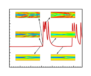Starting from SAR, at first, $C_f$ shows only a small increase, while $\tau _{xx}$ is significantly enhanced; subsequently, $C_f$ shows a rapid increase and falls back to the EIT envelope line, while $\tau _{xx}$ is no longer significantly increased; finally, the flow falls back to SAR from the envelope line along the principal axis, and repeats the above process. Figure 6(b) focuses on the channel flows at ${Wi}=100$. As $SX$ increases, the flow undergoes the evolution process of pure SAR, intermittent flow regime between SAR and EIT, and fully developed EIT, respectively. The flow envelopes almost coincide under the conditions $SX=10$ and $SX=20$. This clearly demonstrates that the flow states obtained by insufficient channel length follow different dynamics from EIT.

Figure 6.

Dynamical and structural evolution cycles of $C_f$ with $\tau _{xx}$ (a) for different $Wi$ at $SX = 8$ and $20$, (b) for different $SX$ at ${Wi} =100$ (the insets present the snapshots of streamwise extension fields $c_{xx}$ for different $SX$, corresponding to the moments a–e in inset 2 of figure 1).

The above phenomenon can also be confirmed from the perspective of the stress balance, budgets of turbulent kinetic energy and elastic energy. The stress balance equation is obtained by the ensemble averaging of the momentum transport equation (2.2) as

(3.2)\begin{equation} {\underbrace{-\overline{u^{\prime}\nu^{\prime}}}_{\overline{\tau_{R}}}+ \underbrace{\frac{1-\beta}{{Re\,Wi}}\,(f(r)\,\overline{c_{xy}}-1)}_{\overline{\tau_{E}}}+ \underbrace{\frac{\beta}{Re}\,\frac{{\rm d}\bar{u}}{{\rm d}y}}_{{\tau_{V}}}=- \underbrace{\frac{{\rm d} p}{{\rm d}\kern0.06em x}{\left(1-\frac {y}{h}\right)}}_{{\tau_{T}}},}\end{equation}

where $\overline {(\cdot )}$ represents the ensemble-averaged variable, $(\cdot )^{\prime }$ is the fluctuating variable, and $(\cdot )^{\prime } = (\cdot )-\overline {(\cdot )}$. Here, $\tau _R$, $\tau _E$, $\tau _V$ and $\tau _T$ are the instantaneous Reynolds stress, elastic stress, viscous shear stress and total stress locally averaged along the streamwise, respectively. Similarly, the elastic energy budget equation can be obtained based on the elastic energy transport equation as

(3.3)\begin{equation} {\int_0^2\underbrace{\overline{\tau_E}\,\frac{\partial\bar{u}}{\partial y}}_{\overline{P_E}}\,\mathrm{d}y- \int_0^2\underbrace{\frac{\overline{f(r)\,\tau_{ii}}}{2\,Wi}}_{\overline{\varepsilon_E}}\,\mathrm{d}y+ \int_0^2\underbrace{\overline{\tau_{ij}^{\prime}\,\frac{\partial u_i^{\prime}}{\partial x_j}}}_{\bar{R}}\,\mathrm{d}y=0,}\end{equation}

where $P_E$, $\varepsilon _E$ and $R$ are the instantaneous terms of the energy production by the elastic stress, the elastic dissipation, and energy exchange between elastic energy and turbulent kinetic energy locally averaged along the streamwise, respectively. Likewise, the budget of turbulent kinetic energy can be obtained as

(3.4)\begin{equation} {\int_0^2\underbrace{-\frac12\,\overline{u^{\prime}\nu^{\prime}}\, \frac{\partial\bar{u}}{\partial y}\,\mathrm{d}y}_{\overline{P_K}}- \int_0^2\underbrace{\frac\beta{Re}\,\overline{\frac{\partial u_i^{\prime}}{\partial x_j}\, \frac{\partial u_i^{\prime}}{\partial x_j}}\,\mathrm{d}y}_{\overline{\varepsilon_K}}- \int_0^2\overline{\underbrace{\tau_{ij}^{\prime}\, \frac{\partial u_i^{\prime}}{\partial x_j}}_{\bar{R}}}\,\mathrm{d}y=0,}\end{equation}

where $P_K$ and $\varepsilon _K$ are the terms of the energy production by the Reynolds stress and the turbulent dissipation locally averaged along the streamwise direction, respectively.

Figure 7 illustrates the averaged budgets of shear stress and turbulent kinetic energy based on the results obtained by different channel lengths. Here, for the intermittent flow regime, the time averaging is performed for the different stages separately. As is shown, different flow patterns present completely different dynamical behaviour. The stage of SAR induced by the centre mode exhibits significant characteristics around the channel centre. For instance, the elastic nonlinear shear stress is lifted up with the peak close to the channel centre (see figure 7a). Although additional nonlinear shear stress is formed relative to laminar flow, it cannot cause a significant increase in flow drag due to the low shear strain rate therein. Compared to negative $\overline {P_K}$, turbulent kinetic energy comes from energy conversion term $\bar {R}$, which is also tightly supported near the channel centre (see figure 7d). However, unlike that of the SAR stage, the stage of EIT exhibits significant near-wall characteristics. For example, the peak of elastic nonlinear shear stress locates much closer to the wall compared to the SAR state (see figure 7b), which can induce high flow drag weighted by high shear strain rate there. The formation of turbulent kinetic energy also relies mainly on energy conversion term $\bar {R}$, but the peak of $\bar {R}$ is very close to the wall. The above phenomena indicate that there exist completely different dynamic mechanisms for EIT from the flow pattern induced by the centre mode.

Figure 7.

Statistical properties for different periods and channel lengths: (a,b) stress distributions in the normal direction based on inner scale; (c,d) turbulent kinetic energy budgets in the normal direction for different channels. Here, 8-SAR and 8-EIT correspond to the results obtained by $SX=8$ in the SAR and EIT stages, respectively.

3.4. Origin and self-sustaining process of EIT

The intermittent flow regime between the SAR and EIT states provides a fabulous opportunity for exploring the origin and self-sustaining mechanism of EIT. To this end, this subsection investigates the structural and dynamical evolution processes of intermittent flow regime obtained at ${Wi}= 100$ with $SX = 8$, and ${Wi} = 40$ with $SX = 5$, respectively. The structural evolution is characterized by the polymer extension structures, and the dynamical evolution process is also evaluated using the the instantaneous budgets of turbulent kinetic energy and elastic energy, as well as shear stress balance analysis, respectively. For the two cases at $Wi=100$ and 40, figures 8 and 9 show several typical moments of EIT from burst to disappearance. The detailed evolution can be found in the supplementary movies. As illustrated in figures 8 and 9 as well as the supplementary movies, the excitation process of EIT can be described as follows.

Figure 8.

The structural and dynamical evolution processes of the intermittent flow regime at ${Wi}= 100$ and $SX = 8$.

Figure 9.

The structural and dynamical evolution processes of the intermittent flow regime at $Wi= 40$ and $SX = 5$.

In the intermittent flow regime of $SX = 8$ and ${Wi} = 100$, starting from the flow with the SAR structure, several near-wall sheet-like streamwise extension structures first appear at $y \approx 0.5$ in the flow (see state 1). These structures gradually grow and extend towards the channel centre (see states 1 and 2). Then they begin to split and modulate the SAR structure (see states 3 and 4), until the SAR structure integrates into the sheet-like extension structures. Subsequently, frequent splitting leads to a rapid increase in $C_f$ as shown in figure 6(a), then the flow develops into the EIT state without the SAR structure (see state 5). The detailed splitting process can be clearly identified in the supplementary movie of Case B from 21 s to 24 s. Due to the above demonstrated computational domain effects on flow states, EIT could not be maintained continuously for a long time as the near-wall extension structures gradually decline (see state 6). Finally, the flow returns to the SAR regime dominated by the centre mode (see state 7). After a long duration of the SAR state, the intervention of wall mode triggers the above process again.

Regarding the instantaneous dynamic evolution process, during the development process from pure SAR state to fully developed EIT state in figure 8, $\tau _{E}$ is significantly higher than $\tau _{R}$, which is responsible for absorbing energy from the average motion and converting it into elastic energy, manifested as a significant elastic energy generation term $P_{E}$. However, the turbulent energy generation $P_{K}$ is weaker, and even has a negative distribution in some regions. Turbulent velocity fluctuations come mainly from energy conversion $R$. The above phenomena indicate that elastic nonlinearity plays a dominant role in the dynamics of SAR and EIT, responsible for their induction and maintenance. Therefore, the origin and self-sustaining mechanism of EIT can be further confirmed by focusing on the elastic nonlinear behaviour in the flow. First, in the pure SAR state (state 7), the dynamic mechanism exhibits centralized characteristics in spatial distribution, such as the peak values of $\tau _{E}$ and $P_{E}$ located at $y \approx 0.75$, and they are approximately linearly distributed at $y<0.6$. Therefore, we believe that SAR is induced and maintained by the centre-mode dynamics. At state 1, with the burst of sheet-like extension structures, near-wall, wall-mode dynamics get involved in the flow, accompanied by local uplift of $\tau _{E}$ and $P_{E}$ at approximately $y = 0.5$. Subsequently, the wall-mode dynamics gradually increases, and the modulated centre-mode dynamics becomes difficult to detect at state 2. In states 3 and 4, the wall-mode dynamics gradually shifts towards the channel wall with high shear strain rates, causing a rapid increase in the flow drag. At state 5 with fully developed EIT, the wall-mode dynamics relatively decreases, and the peak values of $\tau _{E}$ and $P_{E}$ are located at $y \approx 0.2$. It is interesting that at the moment when EIT decays to state 6, $\tau _{E}$ and $P_{E}$ are extremely weak, and energy conversion almost disappears with the decay of EIT at state 6, which cannot provide energy for the maintenance of turbulent fluctuations, indicating the disappearance of elastic nonlinear dynamics. The above phenomena fully demonstrate that EIT originates not from the SAR structure induced by centre-mode dynamics, but rather from the sheet-like extension structures triggered by a wall mode.

Moreover, in the intermittent flow regime of $SX = 5$ and ${Wi} = 40$, as shown in figure 9, it is observed that even starting from the laminar-like flow without SAR structure, the appearance and evolution of near-wall sheet-like structures still closely mirror the process of the case at $SX = 8$, ${Wi} = 100$ in figure 8. They trigger the flow to be unstable and EIT state finally (see state 3). This detailed process can be found in the supplementary movie of Case A from 18 s to 28 s. Similar processes can also be confirmed through the evolution of instantaneous dynamics in figure 9 from state 1 to state 4. Here, the non-existence of peaks near the centreline further corroborates the absence of centre mode.

Therefore, the above results indicate that in the current parameter space, the EIT originates from the near-wall sheet-like structures induced by some wall modes rather than the centre mode, no matter whether there exists centre mode instability or not. From the perspective of dominant structure regeneration, the self-sustaining process of EIT can be described as: small disturbances near the wall induce high extension sheet-like structures, which gradually grow and split under the elastic nonlinearity as well as the fluid inertia, and regenerate new sheet-like structures. The above process continues to occur, maintaining the turbulent state of the flow. Therefore, different from the process of large eddies generating small eddies, and small eddies generating mini eddies in IT, we argue that there exists a different type of structural similarity in EIT: large extension sheets generate small extension sheets, and small extension sheets continues to regenerate as they grow.