
 Mijvib
 VMij





1. Introduction
Understanding the physics of small-scale structures is essential for developing accurate and generalisable turbulence models (Ashurst et al. Reference Ashurst, Kerstein, Kerr and Gibson1987; Ohkitani Reference Ohkitani1993; Pumir Reference Pumir1994; Soria et al. Reference Soria, Sondergaard, Cantwell, Chong and Perry1994). The velocity gradient tensor plays a central role in shaping the dynamics of small-scale structures (Meneveau Reference Meneveau2011; Johnson & Wilczek Reference Johnson and Wilczek2024). The evolution of the velocity gradient tensor following a fluid particle can be studied through: (i) experiments; (ii) direct numerical simulation (DNS) and (iii) a closed set of ordinary differential equations (ODEs) describing velocity gradient dynamics. Performing experimental measurements of velocity gradient dynamics is extremely challenging. To the best of our knowledge, the experimental studies of measuring velocity gradient tensors following a fluid particle are very limited (Xu et al. Reference Xu, Pumir and Bodenschatz2011). Using DNS to access the dynamics of the velocity gradient tensor requires implementing a Lagrangian particle tracker within the simulation, which makes the approach computationally very expensive (Yeung & Pope Reference Yeung and Pope1989; Danish et al. Reference Danish, Suman and Srinivasan2014).
Having a closed set of ODEs that describes the time evolution of the velocity gradient tensor following the motion of a fluid particle offers three main advantages. First, solving these ODEs is computationally cheaper than solving the full set of partial differential equations. Second, their solution directly provides the Lagrangian evolution of the velocity gradient tensor, which is physically more intuitive. Third, such an ODEs system can serve as closures in Lagrangian probability density function (p.d.f.) methods. The Lagrangian p.d.f. methods offer a closure approach for turbulence modelling in inhomogeneous flows (Pope Reference Pope1985).
In incompressible flows, the time evolution of the velocity gradient tensor contains two unclosed terms: the pressure Hessian tensor and the viscous Laplacian tensor. Given the central role of the velocity gradient tensor in turbulence dynamics, modelling these unclosed terms has been a major research focus. A key milestone in this line of research is the work of Vieillefosse (Reference Vieillefosse1982). In his study, the author derived the velocity gradient evolution equation for incompressible flows. In his formulation, the anisotropic part of the pressure Hessian and the viscous effects are neglected. The resulting closed system is known as the restricted Euler equation (REE) model. Despite these simplifications, the REE system can reproduce several important statistical features of turbulence. However, because of the imbalance between the self-stretching term and the isotropic pressure Hessian term, the REE system leads to a finite-time singularity. To address these shortcomings, several modifications have been proposed to incorporate the effects of the anisotropic part of the pressure Hessian tensor and the viscous Laplacian tensor (Cantwell Reference Cantwell1992; Martin et al. Reference Martin, Ooi, Dopazo, Chong and Soria1997; Jeong & Girimaji Reference Jeong and Girimaji2003; Chevillard et al. Reference Chevillard, Meneveau, Biferale and Toschi2008). Among these, the recent fluid deformation (RFD) model is regarded as one of the most successful phenomenological models for velocity gradient dynamics in incompressible turbulence.
Along a similar line of research, there is a growing need for velocity-gradient closure models in compressible turbulence. In compressible flows, the influence of pressure fields on the velocity-gradient dynamics is manifested through two unclosed contributions: the pressure-Hessian tensor, which is inherently symmetric in nature, and the tensor arising from the interaction between the density-gradient and pressure-gradient fields, referred to herein as the baroclinic tensor. The combined effect of these two contributions is represented by the thermodynamic gradient field (TGF) tensor. In earlier studies, the TGF tensor itself was referred to as the pressure-Hessian tensor. Since the earlier terminology was somewhat misleading and may lead to some confusion about the tensor symmetry/non-symmetry, the term TGF tensor is now adopted consistently in the present work. In an incompressible flow field, wherein the density variation is absent, the baroclinic tensor vanishes leading to the TGF tensor becoming the same as symmetric pressure Hessian tensor with density being a constant multiplicative factor.
Unlike incompressible flows, where pressure is governed by the pressure Poisson equation, pressure in compressible flows acts as a thermodynamic variable. Consequently, compressible flows require a separate evolution equation for the thermodynamic gradient field (TGF) tensor as well. The first velocity gradient dynamical model for compressible flows was proposed by Suman & Girimaji (Reference Suman and Girimaji2009), referred to as the homogenised Euler equation (HEE) model. This framework demonstrated reasonable agreement with several features of compressible turbulence dynamics; however, the model is unable to capture the influence of varying Mach numbers. To overcome this limitation, Suman & Girimaji (Reference Suman and Girimaji2011) in their next study derived an explicit evolution equation for the TGF tensor. The authors proposed a coupled system of modelled velocity gradient and TGF tensor evolution equations for compressible flows. At higher turbulent Mach numbers, the baroclinic tensor contributions become more significant. However, the model of Suman & Girimaji (Reference Suman and Girimaji2011) does not include the closures for such baroclinic effects in the TGF tensor evolution equation. To address this, Danish et al. (Reference Danish, Suman and Srinivasan2014) proposed a velocity gradient model that incorporates the influence of the inviscid mechanisms responsible for the generation and evolution of the baroclinic tensor into the proposed TGF tensor evolution equation. Note that the mechanisms responsible for the generation and evolution of the baroclinic tensor were originally referred to as the non-symmetric mechanisms by Danish et al. (Reference Danish, Suman and Srinivasan2014). In the present work, these mechanisms are referred to as baroclinic-tensor-generating mechanisms to better reflect their physical role. The model proposed by Danish et al. (Reference Danish, Suman and Srinivasan2014) is referred to as the new enhanced homogenised Euler equation (N-EHEE) model. The N-EHEE model demonstrated significant improvement over the existing models. Nonetheless, the model relies on the simplified assumption that pressure and density fluctuations remain small compared with their mean values. This assumption does not hold in high-turbulent-Mach-number regimes. These limitations highlight the need for more advanced models capable of accurately capturing the dynamics of the baroclinic tensor contributions in compressible turbulence.
At sufficiently high Mach numbers, turbulent flows start exhibiting various non- equilibrium effects. In particular, in high-temperature regions (
 ${\gt}800\,\mathrm{K}$
), such as those encountered in hypersonic flows and across strong shock fronts, vibrational modes of air molecules become excited. Although these vibrationally excited molecules tend to relax towards equilibrium with the evolving translational–rotational temperature field, the associated relaxation time scale, referred to as the vibrational relaxation time, can be comparable to the characteristic time scale of the turbulent velocity field. This time scale interaction introduces additional complexity into the flow dynamics. Hence, modelling such flows becomes even more challenging. In such regimes, the vibrational energy must be treated as an independent thermodynamic variable and hence evolves separately from the internal energy associated with the temperature field.
Recently, Shikha et al. (Reference Shikha, Srivastava and Sinha2024) proposed a neural-network-based framework to model vibrational non-equilibrium effects in the TGF tensor evolution equation. Their model was evaluated at a single time instant (non-dynamical framework), with all input features extracted directly from DNS data. To the best of our knowledge, however, no dynamical model of velocity-gradient evolution (using neural networks or otherwise) currently exists that explicitly incorporates the effects of vibrational non-equilibrium. In this study, we aim to model vibrational non-equilibrium effects within a dynamical framework for the evolution of velocity gradients.
In recent years, data-driven approaches have gained significant attention in turbulence modelling, offering a promising scope towards more accurate and generalisable closure models (Brunton et al. Reference Brunton, Noack and Koumoutsakos2019). Within the context of velocity-gradient dynamics, the first neural-network-based model was introduced by Parashar et al. (Reference Parashar, Srinivasan and Sinha2020), who employed a tensor-basis neural network (TBNN) framework to model the pressure-Hessian tensor in incompressible turbulence. Subsequent studies have focused on improving neural network architectures and incorporating additional physics-based constraints to enhance the modelling of the pressure-Hessian tensor for incompressible flows (Tian et al. Reference Tian, Livescu and Chertkov2021; Shikha & Sinha Reference Shikha and Sinha2022, Reference Shikha and Sinha2023).
In contrast, machine-learning-based closures for compressible turbulence remain limited. Recently, Shikha et al. (Reference Shikha, Srivastava and Sinha2024) proposed a neural network framework to capture vibrational non-equilibrium effects in the TGF tensor evolution. In the models proposed by Shikha & Sinha (Reference Shikha and Sinha2023) and Shikha et al. (Reference Shikha, Srivastava and Sinha2024), a combination of two distinct neural network architectures is employed to represent two different aspects of the output tensor: its self-normalised form (using the TBNN architecture), which exhibits fairly universal behaviour across different flow fields, and its magnitude, which is comparatively more sensitive across varying flow conditions. Subsequently, Wu & Lele (Reference Wu and Lele2025) have used a similar approach to model the subgrid stress tensor for forced homogeneous isotropic turbulent flows. In this study, we adopt a similar dual neural network-based architecture to develop closure for the inviscid mechanism that is contributing in the generation and the evolution of the baroclinic tensor. In general, such mechanisms are asymmetric in nature. A TBNN designed to represent a second-order tensor requires an appropriate set of tensor bases and scalar invariants. To the best of our knowledge, no prior work has derived a complete set of tensor bases and invariants specifically for modelling a general second-order tensor that is not constrained to be symmetric. To this end, we aim to derive a complete set of tensor bases and scalar invariants suitable for representing an arbitrary second-order tensors without symmetry constraints.
Furthermore, all existing neural-network-based models for velocity-gradient closures (both incompressible and compressible) have been assessed solely through a priori evaluations, wherein the input quantities are extracted directly from DNS databases at a given time instant and the models are evaluated in a non-dynamical setting. As a result, these studies do not provide a dynamical closure of velocity-gradient evolution, in which both the velocity-gradient tensor and the neural-network inputs evolve simultaneously through a coupled system of ODEs. To the best of our knowledge, no existing study has developed a dynamical velocity-gradient framework in which neural-network-predicted closures are embedded directly into the governing evolution equations and integrated over time. The present work addresses this gap by constructing a fully dynamical velocity-gradient framework that incorporates neural-network predictions within a closed system of ODEs, thereby providing access to the continuous evolution of the velocity-gradient tensor along fluid-particle trajectories. Modelling the velocity-gradient dynamics of compressible flows with vibrational non-equilibrium effects using a single neural-network architecture can be particularly challenging because multiple physical mechanisms contribute simultaneously to the flow evolution. Therefore, the present framework employs separate neural-network closures for distinct physical mechanisms governing the velocity-gradient and TGF tensor dynamics. In particular, vibrational non-equilibrium effects are represented through a dedicated neural-network closure, while the contributing mechanism in the baroclinic tensor evolution is modelled independently. This modular strategy reduces the complexity of the learning task, allows each network to focus on a specific physical mechanism, and improves the interpretability and robustness of the resulting dynamical framework. Motivated by the identified research gaps and the associated challenges, the present study pursues the following novel objectives.
-
(i) To develop an apt tensor-basis and invariants-based neural-network closure for the inviscid mechanism contributing to the baroclinic tensor generation and evolution, thereby overcoming the limitations of the existing phenomenological model proposed by Danish et al. (Reference Danish, Suman and Srinivasan2014).
-
(ii) To incorporate recently developed neural-network-based closures for the inviscid baroclinic tensor generating mechanism and vibrational non-equilibrium mechanisms into a dynamical velocity-gradient framework.
-
(iii) To formulate a novel hybrid dynamical velocity-gradient model (a closed set of ODEs) for compressible flows, in which unclosed terms are represented using a combination of phenomenological modelling and neural-network-based closures.
-
(iv) To assess the performance of the proposed model across a wide range of flow regimes, spanning low- to high-turbulent-Mach-number conditions, including regions with active vibrational non-equilibrium effects by making comparisons with DNS data as well as with existing models of compressible velocity gradient dynamics.
This paper is organised into ten sections. Section 2 introduces the evolution equation of the velocity gradient and pressure Hessian tensors for compressible flows. Section 3 gives a brief review of the existing model of velocity gradient dynamics in compressible flows. Sections 4–7 discuss the enhancements and modelling strategies employed in the current study. Section 7 gives a summary of the newly proposed model of velocity gradient tensor in compressible flows. Section 8 presents the non-dimensionalised form of the model. Section 9 provide an extensive performance assessment of the model across different flow conditions. Finally, § 10 concludes the paper with a brief summary.
2. Evolution equations of velocity gradient dynamics in compressible turbulence
For a calorically perfect compressible fluid, the Navier–Stokes equation set can be written as follows:
 \begin{equation} \frac {\partial {\rho }}{\partial {t}} + {V_k} \frac {\partial {\rho }}{\partial {x_k}}= -\rho \frac {\partial {V_{k}}}{\partial {x_k}}, \end{equation}
 \begin{equation} \frac {\partial {V_i}}{\partial {t}} + {V_k} \frac {\partial {V_i}}{\partial {x_k}}= -\frac {1}{\rho } \frac {\partial {p}}{\partial {x_i}} + \frac {1}{\rho }\frac {\partial {\sigma _{ik}}}{\partial {x_k}}, \end{equation}
where
 $V_i$
,
 $t$
and
 $x_i$
denote the velocity, time and spatial coordinates in the Eulerian frame of reference, respectively. The symbol
 $p$
represents pressure,
 $\rho$
represents density and
 $\sigma _{ik}$
represents the viscous stress tensor. For a Newtonian fluid, the viscous stress is given by
 \begin{equation} \sigma _{ij} = \rho \, \mu \left ( A_{ij} + A_{ji} - \frac {2}{3} A_{kk} \delta _{ij} \right )\!, \end{equation}
where
 $\delta _{ij}$
is the Kronecker delta. The evolution of the velocity gradient tensor
 $(A_{ij}= {\partial V_{\!j}}/{\partial x_{i}})$
is derived by taking the material derivative (
 $ {\rm D}/{{\rm D}t}\equiv {\partial }/{\partial t} + u_{i} ({\partial }/{\partial x_{i}})$
) of the momentum equation (2.2) (Suman & Girimaji Reference Suman and Girimaji2011):
 \begin{align} \frac {{\rm D} A_{ij}}{{\rm D} t} = - A_{ik}A_{kj} -\underbrace {\frac {\partial }{\partial x_{\!j}} \left ( \frac {1}{\rho }\frac {\partial p}{\partial x_{i}} \right )}_{P_{ij}} + \underbrace {\mu \frac {\partial ^{2} A_{ij}}{\partial x_{k} \partial x_{k}} + \frac {\mu }{3}\frac {\partial ^{2} A_{kk}}{\partial x_{i} \partial x_{\!j}}-\frac {\mu }{\rho }\frac {\partial \rho }{\partial x_{\!j}} \left ( \frac {\partial A_{ik}}{\partial x_{k}} + \frac {1}{3}\frac {\partial A_{kk}}{\partial x_{i}}\right )}_{\varGamma _{ij}}, \end{align}
where
 $\mu$
denotes the kinematic viscosity. The left-hand side of (2.4) represents the Lagrangian evolution of the velocity gradient tensor, i.e. its rate of change following a fluid particle. The right-hand side contains three terms that govern this evolution. The first term,
 $-A_{ik}A_{kj}$
, is the self-stretching term. It depends solely on the velocity gradient tensor itself and is therefore mathematically closed. The second term,
 $P_{ij}$
, denotes the thermodynamic gradient field tensor (TGF tensor). In earlier studies, this term was referred to as the pressure-Hessian tensor. However, since the tensor incorporates the effects of density and pressure gradients in addition to the pressure Hessian itself, the term thermodynamic gradient field tensor is adopted in the present work to more accurately reflect its physical behaviour. The third term,
 $\varGamma _{ij}$
, is the viscous Laplacian tensor. Unlike the self-stretching term, the TGF tensor (
 $P_{ij}$
) and the viscous Laplacian tensors (
 $\varGamma _{ij}$
) are mathematically unclosed and inherently non-local. Consequently, closing (2.4) requires either deriving separate evolution equations for these terms or modelling them explicitly. In compressible flows, the term
 $P_{ij}$
needs its own evolution equation, which can be obtained from the evolution of the internal energy,
 $e = C_{v} T$
, where
 $C_{v}$
is the specific heat at constant volume and
 $T$
is the thermodynamic temperature. Suman & Girimaji (Reference Suman and Girimaji2011) derived the evolution equation for the
 $\boldsymbol{P}$
tensor in compressible flows without accounting for vibrational non-equilibrium effects. Later, Srivastava et al. (Reference Srivastava, Bhat and Sinha2024) incorporated vibrational non-equilibrium effects into the pressure-Hessian evolution equation
 \begin{align} \frac {{\rm D}P_{ij}}{{\rm D}t} =& \underbrace {-A_{kj}P_{ik}-A_{ki}P_{kj}-(n-1) A_{kk}P_{ij}}_{(I_{ij})} \nonumber \\ & \underbrace {-\frac {n}{\rho }\left (\frac {\partial A_{kk}}{\partial x_{\!j}}\ \frac {\partial p}{\partial x_i} + \frac {\partial A_{kk}}{\partial x_i} \frac {\partial p}{\partial x_{\!j}}\right )}_{\textit{II}_{ij}} \underbrace {-\frac {1}{\rho } \frac {\partial A_{ki}}{\partial x_{\!j}} \frac {\partial P} {\partial x_{k}}}_{\textit{III}_{ij}} \underbrace {-\frac {np}{\rho }\frac {\partial ^2A_{kk}}{\partial x_{i}\partial x_{\!j}}}_{\textit{IV}_{ij}}\nonumber \\ & \qquad \underbrace {+\frac {1}{\rho }\frac {\partial A_{kk}}{\partial x_{\!j}}\frac {\ \partial p}{\partial x_i} +\frac {np}{\rho ^{2}}\frac {\partial A_{kk}}{\partial x_i}\frac {\ \partial \rho }{\partial x_{\!j}}}_{(V_{ij})}\nonumber \\ & \quad \underbrace {+\left (\frac {n-1}{R}\right )\ \frac {\partial }{\partial x_{\!j}}\left \{\frac {1}{\rho }\frac {\partial ^2}{\partial x_i\partial x_k}\left [k\ \frac {\partial }{\partial x_k}\left (\frac {p}{\rho }\right )\right ]\right \}}_{(\textit{VI}_{ij})} \nonumber \\ & \ +\underbrace {(n-1) \frac {\partial }{\partial x_{\!j}}\left [\frac {1}{\rho }\ \frac {\partial \sigma _{km}}{\partial x_i} A_{km}+\frac {1}{\rho }\sigma _{km}\ \frac {\partial A_{km}}{\partial x_i}\right ]}_{(\textit{VII}_{ij})} \nonumber \\& + \underbrace {(n-1)\frac {\partial }{\partial x_{\!j}}\left [\frac {1}{\rho }\frac {\partial }{\partial x_i}\left (\frac {\rho {e}_{v}}{\tau _{vib}}\right )\right ]}_{(\textit{VIII}_{ij})} - \underbrace {(n-1)\frac {\partial }{\partial x_{\!j}}\left [\frac {1}{\rho }\frac {\partial }{\partial x_i}\left (\frac {\rho {e}_{v}^{*}}{\tau _{vib}}\right )\right ]}_{(\textit{IX}_{ij})}, \end{align}
here,
 $k$
denotes the thermal conductivity. The symbol
 $e_{\nu }$
denotes the vibrational non-equilibrium energy per unit mass, while
 $e_{\nu }^{*}$
denotes the vibrational energy per unit mass in equilibrium with the local temperature
 $T$
. The vibrational non-equilibrium energy relaxes towards
 $e_{\nu }^{*}$
on a characteristic time scale
 $\tau _{vib}$
, which is referred to as the vibrational relaxation time. Following Vincenti et al. (Reference Vincenti, Kruger, Charles and Teichmann1966), the equilibrium vibrational energy per unit mass is expressed as
 \begin{equation} e_{\nu }^{*} = \frac {\dfrac {h \nu }{k_{B} T}}{\exp \!\left ( \dfrac {h \nu }{k_{B} T} \right ) - 1}\, \textit{RT}, \end{equation}
where
 $R$
is the gas constant,
 $h$
is Planck’s constant,
 $\nu$
is the molecular vibrational frequency and
 $k_{B}$
is Boltzmann’s constant.
The terms written on the right-hand side of (2.5) are grouped according to their physical significance, and each group corresponds to a distinct mechanism governing the evolution of the
 $P_{ij}$
tensor. The group
 $I_{ij}$
mechanisms represent the direct interaction of the
 $P_{ij}$
with the
 $A_{ij}$
tensor and are therefore mathematically closed. The mechanism groups
 $\textit{II}_{ij}$
–
 $V_{ij}$
are inviscid and non-local in nature, capturing interactions involving the gradients of
 $A_{kk}$
and pressure
 $(p)$
. In particular, the term
 $\textit{IV}_{ij}$
contains the factor
 $ {n p}/{\rho }$
, which highlights the influence of acoustic time scales or Mach number effects (Suman & Girimaji Reference Suman and Girimaji2011). Mechanisms
 $\textit{VI}_{ij}$
and
 $\textit{VII}_{ij}$
describe non-local contributions arising from thermal conduction and viscous heating, respectively. Mechanisms
 $\textit{VIII}_{ij}$
and
 $\textit{IX}_{ij}$
account for the influence of vibrational non-equilibrium on the evolution of the pressure Hessian. Due to the presence of higher-order gradients of the velocity gradient and density fields, the mechanisms
 $\textit{II}_{ij}$
–
 $\textit{IX}_{ij}$
are mathematically unclosed. Consequently, closing the
 $P_{ij}$
evolution equation requires appropriate modelling of these mechanisms (
 $\textit{II}_{ij}$
–
 $\textit{IX}_{ij}$
).
The
 $P_{ij}$
tensor can be decomposed into two parts as
 \begin{equation} P_{ij} \equiv \frac {\partial }{\partial x_{\!j}}\left ( \frac {1}{\rho }\frac {\partial p}{\partial x_{i}} \right ) = \underbrace {\frac {1}{\rho }\frac {\partial ^{2} p}{\partial x_{\!j}\partial x_{i}}}_{H_{ij}} - \underbrace {\frac {1}{\rho ^{2}}\frac {\partial \rho }{\partial x_{\!j}}\,\frac {\partial p}{\partial x_{i}}}_{B_{ij}} , \end{equation}
such that
 \begin{equation} P_{ij} = H_{ij} - B_{ij}. \end{equation}
Here, the tensor
 $\rho H_{ij}$
is indeed the pressure-Hessian tensor. The tensor
 $B_{ij}$
is referred to as the baroclinic tensor because it arises from the interaction between the density-gradient and pressure-gradient fields. The pressure-Hessian tensor is inherently symmetric, whereas the baroclinic tensor is generally asymmetric. In the work of Danish et al. (Reference Danish, Suman and Srinivasan2014), the tensors
 $H_{ij}$
and
 $B_{ij}$
were referred to as the symmetric and non-symmetric pressure-Hessian components, respectively. In the incompressible-flow limit, density gradients vanish. Consequently, the term
 $P_{ij}$
is merely
 $H_{ij}$
and
 $B_{ij} =0$
.
3. Existing model for velocity-gradient dynamics in compressible turbulence: a brief review
In this section, we provide a brief review of the existing model for compressible velocity-gradient dynamics proposed by Danish et al. (Reference Danish, Suman and Srinivasan2014). In this framework, a phenomenological closure strategy is employed to model the unclosed terms appearing in the evolution equations of the
 $A_{ij}$
(2.4) and the
 $P_{ij}$
tensors (2.5). The resulting formulation is summarised as
 \begin{equation} \frac {{\rm d}A_{ij}}{{\rm d}t} = -A_{ik}A_{kj} -P_{ij} -\frac {C_{\! pq}C_{\! pq}}{3\tau _{v}} \left ( A_{ij} + \frac {A_{kk}}{3C_{\! pq}C_{\! pq}}C_{ri}C_{rj} \right )\!, \end{equation}
 \begin{equation} \frac {{\rm d}P_{ij}}{{\rm d}t} = -\left ( P_{ij} + \frac {A_{lm}A_{ml}}{C_{\! pq}C_{\! pq}}C_{ri}C_{rj} \right )\frac {c}{L} -\frac {C_{\! pq}C_{\! pq}}{3\tau _{p}}P_{ij} +A_{kk}\sqrt {P_{mn}P_{mn}} \frac {C_{ij}}{\sqrt {C_{qr}C_{qr}}}, \end{equation}
 \begin{equation} \boldsymbol{M} \equiv \boldsymbol{C}^{-1}, \end{equation}
 \begin{equation} \frac {{\rm d}M_{ij}}{{\rm d}t} = A_{ik}M_{kj}, \end{equation}
 \begin{equation} L = \max \left [ \frac {L_{0}}{\sqrt {C_{\! pq}C_{\! pq}/3}}, \frac {L_{0}}{\sqrt {\tau _{\nu }A}} \right ]\!, \quad \text{where } \quad A=\sqrt {A_{ij}A_{ij}}. \end{equation}
Equations (3.1)–(3.5) constitute a closed system of 27 ODEs governing the Lagrangian evolution of the velocity-gradient tensor and the
 $P_{ij}$
tensor in compressible turbulence. This ODE system is referred to as the new enhanced homogenised Euler equation (N-EHEE) model. Here,
 $c$
denotes the speed of sound and
 $L$
represents a characteristic fluid length scale, with
 $L_{0}\equiv L(t=0)$
. The term
 $C_{ij}$
represents the deformation-gradient tensor, which is defined as
 \begin{equation} C_{ij} \equiv \frac {\partial X_{i}}{\partial x_{\!j}}, \end{equation}
where
 $x$
and
 $X$
denote the Eulerian and Lagrangian coordinates of a fluid particle, respectively. A detailed derivation and physical interpretation of various terms can be found in the original work of Danish et al. (Reference Danish, Suman and Srinivasan2014).
4. Enhancements and new modelling suggestions
The N-EHEE model relies on two key simplifying assumptions: (i) thermodynamic fluctuations are sufficiently small compared with their mean values and (ii) the thermodynamic variables follow a polytropic process. Previous DNS studies (Sarkar et al. Reference Sarkar, Erlebacher, Hussaini and Kreiss1991; Blaisdell et al. Reference Blaisdell, Mansour and Reynolds1993) indicate that these assumptions remain valid up to a turbulent Mach number of approximately
 $0.5$
. However, at higher Mach numbers, thermodynamic fluctuations become significant and deviations from polytropic behaviour increase, thereby limiting the applicability of the N-EHEE model. Moreover, the model does not incorporate any closure for vibrational non-equilibrium effects. Being aware of the limitations of the existing model (3.1)–(3.5), the present study aims to develop an improved formulation that adapts to varying flow conditions, including high-turbulent Mach numbers, and accounts for the effects of vibrational non-equilibrium.
In the current modelling framework, separate evolution equations are formulated for the
 $\boldsymbol{H}$
and
 $\boldsymbol{B}$
tensors (2.7). Having these two separate governing equations allows the already-modelled component of the
 $\boldsymbol{P}$
tensor to serve as an input for predicting the unknown component. On the right-hand side of (2.5), after identifying the distinct effects governing mechanisms, we develop their respective closure forms and incorporate them into the modelled evolution equations for the
 $\boldsymbol{H}$
and
 $\boldsymbol{B}$
tensor, consistent with their underlying physical nature.
We first aim to modify the already-modelled mechanisms as per the new modelling framework. In this, we first focus on modifying the closure of mechanism
 $\textit{IV}_{ij}$
proposed by Danish et al. (Reference Danish, Suman and Srinivasan2014). In their formulation (3.2), the mechanism
 $\textit{IV}_{ij}$
(2.5) is modelled such that the
 $P_{ij}$
tensor relaxes towards its incompressible counterpart over the acoustic time scale:
 $L/c$
. In the present work, owing to the availability of separate evolution equations for the
 $\boldsymbol{H}$
and
 $\boldsymbol{B}$
tensors, the existing model of the
 $\textit{IV}_{ij}$
(2.5) mechanism is modified as
 \begin{align} -\frac {np}{\rho }\frac {\partial ^2 A_{kk}}{\partial x_i \partial x_{\!j}} \;\equiv \; -\left ( P_{ij} + \frac {A_{lm}A_{ml}}{C_{\! pq}C_{\! pq}}C_{ri}C_{rj} \right )\frac {c}{L} \\[-12pt]\nonumber \end{align}
 \begin{align} \equiv -\left ( H_{ij} + \frac {A_{lm}A_{ml}}{C_{\! pq}C_{\! pq}}\, C_{ri} C_{rj} \right ) \frac {c}{L}+B_{ij}\frac {c}{L}. \end{align}
Next, we modify the closure of the thermal conduction processes denoted by the
 $\textit{VI}_{ij}$
mechanism in (2.5), contributing to the
 $\boldsymbol{P}$
tensor (Danish et al. Reference Danish, Suman and Srinivasan2014). Upon decomposing the existing model of the thermal heating mechanisms explicitly into their
 $\boldsymbol{H}$
and
 $\boldsymbol{B}$
contributing parts, the resulting expression is written as
 \begin{align} \left (\frac {n-1}{R}\right ) \frac {\partial }{\partial x_{\!j}} \left \{ \frac {1}{\rho } \frac {\partial ^2}{\partial x_i\partial x_k} \left [ k\frac {\partial }{\partial x_k}\left (\frac {p}{\rho }\right ) \right ] \right \} \equiv - \frac {C_{\! pq}C_{\! pq}}{3\tau _{p}}P_{ij} = - \frac {C_{\! pq}C_{\! pq}}{3\tau _{p}}(H_{ij}-B_{ij}). \end{align}
The mechanism
 $I_{ij}$
(2.5) represents the direct interaction between the
 $\boldsymbol{A}$
and
 $\boldsymbol{P}$
tensors, and hence it is mathematically closed. We directly use the various terms involved in the mechanism
 $I_{ij}$
(2.5) in our model. For this, we decompose the exact form of the mechanism
 $I_{ij}$
(2.5) using (2.8). Accordingly, the mechanism
 $I_{ij}$
(2.5) can be expressed as the sum total of two parts
 \begin{align} -A_{kj} P_{ik} -A_{ki} P_{kj} -(n-1) A_{kk} P_{ij}&=& \\ \nonumber \left [-A_{kj} H_{ik} -A_{ki} H_{kj} -(n-1) A_{kk} H_{ij} \right ] &+\left [A_{kj} B_{ik} +A_{ki} B_{kj} +(n-1) A_{kk} B_{ij} \right ]\!. \end{align}
It is desirable to retain both the
 $\boldsymbol{H}$
and
 $\boldsymbol{B}$
tensors contributions arising from the decomposition of these exact terms (mechanism
 $I_{ij}$
, as evident in (4.4)). However, prior modelling experience suggests that including the
 $\boldsymbol{H}$
contributions of the mechanism
 $I_{ij}$
(2.5) in the evolution equation for the
 $\boldsymbol{H}$
tensor compromises the model’s ability to maintain the correct behaviour of the velocity divergence in low-Mach regions (wherein,
 $A_{ii}$
must be negligible at all times for all fluid elements). Consequently, the
 $\boldsymbol{H}$
contributions of these terms are neglected, and only the
 $\boldsymbol{B}$
of the mechanism
 $I_{ij}$
is retained and incorporated into the evolution equation of the
 $\boldsymbol{B}$
tensor. The resulting expression for the
 $I_{ij}$
(2.5) tensor closure is hence approximated as
 \begin{equation} -A_{kj} P_{ik} -A_{ki} P_{kj} -(n-1) A_{kk} P_{ij} \approx A_{kj} B_{ik} +A_{ki} B_{kj} +(n-1) A_{kk}B_{ij}. \end{equation}
With the closures for the various mechanisms proposed in this section (as given in (4.5), (4.1), (4.3)), the evolution equations governing the
 $\boldsymbol{H}$
and
 $\boldsymbol{B}$
tensors can be written as
 \begin{align} \frac {{\rm d}H_{ij}}{{\rm d}t}=-\left ( H_{ij} +\frac {A_{lm}A_{ml}}{C_{\! pq}C_{\! pq}} C_{ri}C_{rj}\right ) \frac {c}{L} - \frac {C_{\! pq}C_{\! pq}}{3\tau _{p}} H_{ij}+M_{ij}^{vib}, \\[-12pt]\nonumber \end{align}
 \begin{align} \frac {{\rm d}B_{ij}}{{\rm d}t}= -A_{kj}B_{ik} -A_{ki}B_{kj} -(n-1)A_{kk}B_{ij}-B_{ij}\frac {c}{L} -V_{M_{ij}} -\frac {C_{\! pq}C_{\! pq}}{3\tau _{p}} B_{ij}. \end{align}
The term
 $M_{ij}^{{vib}}$
, appearing in (4.6), represents the modelled contribution of the symmetric component of the vibrational non-equilibrium mechanism denoted by
 $\textit{VIII}_{ij}+\textit{IX}_{ij}$
(2.5). Although the vibrational non-equilibrium mechanism is inherently asymmetric in nature, DNS investigations by Shikha et al. (Reference Shikha, Srivastava and Sinha2024) indicate that the magnitude of the antisymmetric component of the vibrational non-equilibrium tensor remains negligible for flow fields with turbulent Mach numbers (
 $M_t$
) up to
 $0.5$
. In the present modelling framework, only the symmetric component of the vibrational non-equilibrium mechanism is incorporated into the evolution equation of the
 $\boldsymbol{H}$
tensor. No explicit representation of the vibrational non-equilibrium mechanism effects, either symmetric or antisymmetric, is included in the evolution of the
 $\boldsymbol{B}$
tensor. The development of a neural-network-based closure for the antisymmetric vibrational non-equilibrium mechanism, which may require addressing further modelling complexities, is left for future work. Addressing these complexities may require performing detailed analysis employing a high-Mach-number DNS database before any modelling attempts can be made, and is out of the scope of this study.
The term
 $V_{M_{ij}}$
, used in (4.7), denotes the modelled representation of the
 $V_{ij}$
mechanism identified in (2.5). The mechanism
 $V_{ij}$
(2.5) is the inviscid mechanism which contributes to the generation of
 $\boldsymbol{B}$
tensor even when the initial velocity-gradient and TGF tensors do not contain density-gradient effects (i.e.
 $B_{ij}=0, \, at \, t=0$
). This behaviour arises from the explicit involvement of density-gradient-related terms within the
 $V_{ij}$
mechanism. To close (4.6) and (4.7), appropriate closure models are required for the remaining unclosed mechanisms, namely
 $ M_{ij}^{vib}$
and
 $ V_{M_{ij}}$
. In the following two sections, we develop closure models for the vibrational non-equilibrium mechanism and the
 $V_{ij}$
mechanism, respectively.
5. Model of
 $\boldsymbol{M_{ij}^{vib}}$

For the first time, in this work, we incorporate a model of vibrational non-equilibrium mechanisms into a dynamical velocity-gradient framework. To this end, we build upon the modelling strategy proposed by Shikha et al. (Reference Shikha, Srivastava and Sinha2024). In that work, a physics-assisted neural-network model was developed to represent the non-dimensional form of the vibrational non-equilibrium mechanisms (
 $\textit{VIII}_{ij}$
+
 $\textit{IX}_{ij}$
) appearing in the
 $P_{ij}$
evolution (2.5). The non-dimensionalisation was carried out using local magnitudes of the
 $A_{ij}$
and the
 $P_{ij}$
tensors:
 \begin{align} \varPi _{ij}= \frac {1}{\epsilon \sqrt {P_{mn}P_{mn}}} \left [ (n-1)\frac {\partial }{\partial x_{\!j}} \left \{ \frac {1}{\rho }\frac {\partial }{\partial x_{i}} \left ( \frac {\rho e_{v}}{\tau _{vib}}\right ) \right \} - (n-1)\frac {\partial }{\partial x_{\!j}} \left \{ \frac {1}{\rho }\frac {\partial }{\partial x_{i}} \left ( \frac {\rho e_{v}^{*}}{\tau _{vib}}\right ) \right \} \right ]\!, \end{align}
where
 $\epsilon =\sqrt {A_{ij}A_{ij}}$
. By definition, the tensor
 $\boldsymbol{\varPi }$
(5.1) is asymmetric. To simplify the modelling strategy, Shikha et al. (Reference Shikha, Srivastava and Sinha2024) decomposed
 $\boldsymbol{\varPi }$
into its symmetric and antisymmetric components as
 \begin{equation} \boldsymbol{\varPi }= \boldsymbol{^{s}\varPi } + \boldsymbol{^{a}\varPi }. \end{equation}
DNS-based analyses performed by Shikha et al. (Reference Shikha, Srivastava and Sinha2024) demonstrated that, for the range of parameters considered in their study (initial turbulent Mach number up to
 $0.5$
), the magnitude of the antisymmetric component (
 $\boldsymbol{^{a}\varPi }$
) is negligible compared with that of the symmetric component (
 $\boldsymbol{^{s}\varPi }$
). Based on this observation, the following approximation was adopted:
 \begin{equation} \boldsymbol{\varPi } \approx \boldsymbol{^{s}\varPi }. \end{equation}
Under this approximation, the vibrational non-equilibrium contribution is modelled as a purely symmetric tensor. The resulting closure for
 $\boldsymbol{\varPi }$
is referred to as the invariants-based vibrational non-equilibrium model (IBVM).
To model
 $\varPi _{ij}$
, the IBVM employs two neural networks. The first network predicts the self-normalised tensor, denoted by
 $\widehat {\varPi }_{ij}$
. The second network predicts the scalar magnitude, denoted by
 $\varPhi$
, of the non-dimensional vibrational non-equilibrium tensor. The self-normalised tensor
 $\widehat {\varPi }_{ij}$
and the magnitude
 $\varPhi$
are defined as follows:
 \begin{equation} \widehat {\varPi }_{ij} =\frac {\varPi _{ij}}{\sqrt {\varPi _{mn}\varPi _{mn}}},\quad\varPhi =\sqrt {\varPi _{ij}\varPi _{ij}}, \end{equation}
where
 $\sqrt {\widehat {\varPi }_{ij}\widehat {\varPi }_{ij}}=1$
.
The IBVM adopts the TBNN framework to predict the self-normalised vibrational tensor
 $\widehat {\varPi }_{ij}$
. In this approach, tensor bases and scalar invariants are constructed using the normalised pressure-Hessian tensor
 $\boldsymbol{\widehat {H}}$
, the normaliesd rotation-rate tensor
 $\boldsymbol{{W}}$
and the locally defined Damköhler number
 $D_{m}$
. The normalised symmetric pressure-Hessian tensor is defined as
 \begin{equation} \boldsymbol{\widehat {H}}=\frac {\boldsymbol{H}}{|\boldsymbol{H}|}, \end{equation}
where
 $|\boldsymbol{H}|=\sqrt {H_{ij}H_{ij}}$
. The normalised rotation-rate tensor is obtained from the self-normalised velocity-gradient tensor (
 $\boldsymbol{a}=\boldsymbol{A}/|\boldsymbol{A}|$
, where
 $|\boldsymbol{A}|=\sqrt {A_{ij}A_{ij}}$
) as
 \begin{equation} \boldsymbol{W}=\frac {\boldsymbol{a}-\boldsymbol{a}^{T}}{2}. \end{equation}
The Damköhler number is a key non-dimensional parameter characterising vibrational non-equilibrium effects. It is traditionally defined as the ratio of the large-eddy turnover time to the vibrational relaxation time (Khurshid & Donzis Reference Khurshid and Donzis2019; Srivastava et al. Reference Srivastava, Bhat and Sinha2024). Shikha et al. (Reference Shikha, Srivastava and Sinha2024), introduced locally defined Damköhler number
 $D_{m}$
given by
 \begin{equation} D_{m}=\frac {1}{\tau _{{vib}}\sqrt {A_{ij}A_{ij}}}, \end{equation}
where
 $(A_{ij}A_{ij})^{-1/2}$
represents the characteristic time scale of the motion of a local fluid element. The symbol
 $\tau _{{vib}}$
represents the vibration relaxation time. The modelled representation of the
 $\widehat {\varPi }_{ij}$
tensor is given as
 \begin{equation} \boldsymbol{\widehat {\varPi }}^{\textit{IBVM}} = \mathcal{G}_{ibvm} (\boldsymbol{\widehat {H}}, \boldsymbol{W}, D_m), \end{equation}
where
 $\mathcal{G}^{ibvm}$
is the modelled mapping, which is accessible in the form of weights and biases saved in the trained neural network. The reader is referred to the original paper by Shikha et al. (Reference Shikha, Srivastava and Sinha2024) for further details of the tensor bases and invariants employed in this model.
The second neural network predicts the scalar magnitude
 $\varPhi$
of the non-dimensional vibrational tensor. To predict the magnitude
 $\varPhi$
, IBVM model (Shikha et al. Reference Shikha, Srivastava and Sinha2024) used a fully connected simple neural network with input quantities in the form of the first and third invariants (
 $I_{r1}\, \text{and} \,I_{r3}$
) of the
 $\boldsymbol{\widehat {H}}$
tensor (5.5), the locally defined model Damköhler number
 $D_{m}$
(5.7) and the local compressibility parameters such as: (i) the dilatation rate (
 $a_{ii}$
) and (ii) the rate of change of local dilatation rate (
 $\delta$
). These parameters are mathematically defined as
 \begin{equation} a_{ii}=\frac {A_{ii}}{\epsilon }, \quad \delta =\frac {-A_{ij}A_{ji}-H_{ii}+B_{ii}}{\epsilon ^{2}}, \end{equation}
where
 $\epsilon =\sqrt {A_{ij}A_{ij}}$
. The invariants of
 $\boldsymbol{\widehat {H}}$
are defined as
 \begin{equation} I_{r1}=\text{Tr}\big(\boldsymbol{\widehat {H}}\big), \end{equation}
 \begin{equation} I_{r2}=\frac {1}{2}\Big (I_{r1}^{2}-\text{Tr}\Big(\boldsymbol{\widehat {H}}^{2}\Big)\Big ), \end{equation}
 \begin{equation} I_{r3}=\frac {1}{3}\Big (-I_{r1}^{3}+3I_{r1}I_{r2}-\text{Tr}\Big(\boldsymbol{\widehat {H}}^{3}\Big)\Big ), \end{equation}
where
 $\text{Tr}$
means trace of a tensor. Hence, the closure of
 $\varPhi$
is written as
 \begin{equation} \varPhi ^{\textit{IBVM}}= \mathcal{F}_{ibvm}(a_{ii}, \delta , D_{m}, I_{r1}, I_{r3}), \end{equation}
where
 $\mathcal{F}_{ibvm}$
is the modelled mapping, which is obtained in the form of the weights and biases of the trained neural network.
The final non-dimensionalised vibrational non-equilibrium tensor is obtained by combining the outputs of the two networks ((5.8) and (5.11)) as
 \begin{equation} \boldsymbol{\varPi }^{\textit{IBVM}}=\widehat {\boldsymbol{\varPi }}^{\textit{IBVM}}\,\varPhi ^{\textit{IBVM}}. \end{equation}
We aim to develop a dynamic model having vibrational non-equilibrium effects that relax to the model of vibrational equilibrium flows, in the limit of
 \begin{equation} e_{\nu }=e_{\nu }^{*}. \end{equation}
The symbol
 $e_{\nu }$
denotes the vibrational non-equilibrium energy per unit mass, while
 $e_{\nu }^{*}$
(2.6) denotes the vibrational energy per unit mass in equilibrium with the local temperature. To bring this feature into our dynamical model, we define a new non-dimensional parameter,
 $\xi _{m}$
as
 \begin{equation} \xi _{m}= \frac {e_{\nu }}{e_{\nu }^{*}}. \end{equation}
Note that flow regimes in vibrational equilibrium always satisfy
 $\xi _{m}=1$
. Using the locally available quantities
 $\sqrt {A_{pq}A_{pq}}\,\text{and}\, \sqrt {P_{mn}P_{mn}}$
, we write the modelled representation of the vibrational non-equilibrium mechanism (
 $M_{ij}^{vib}$
) as
 \begin{equation} M_{ij}^{vib}= \frac {(1-{\xi _{m}}_{0})}{(1+\xi _{m})}\,\boldsymbol{\varPi }^{\textit{IBVM}}\ \sqrt {A_{pq}A_{pq}}\sqrt {P_{mn}P_{mn}}, \end{equation}
where
 ${\xi _{m}}_{0}=\xi _{m}(t=0)$
. We propose to model the evolution process of
 $\xi _{m}$
inspired by the Landau–Teller model of Vincenti et al. (Reference Vincenti, Kruger, Charles and Teichmann1966) for the source term of the evolution equation of vibrational energy per unit mass. The proposed evolution equation of
 $\xi _{m}$
is written as
 \begin{equation} \frac {{\rm d}\xi _{m}}{{\rm d}t}=-\frac {\xi _{m}-1}{\tau _{t{vib}}}. \end{equation}
Following this framework, the proposed model tends to the vibrational equilibrium case when
 ${\xi _{m}}_{0}$
becomes unity. With these extensions, the evolution equation for the
 $\boldsymbol{H}$
tensor can be written as
 \begin{align} \frac {{\rm d}H_{ij}}{{\rm d}t} =&- \left ( H_{ij} + \frac {A_{lm} A_{ml}}{C_{\! pq} C_{\! pq}} \, C_{ri} C_{rj} \right ) \frac {c}{L} - \frac {C_{\! pq} C_{\! pq}}{3 \tau _{p}} \, H_{ij} \nonumber \\[5pt] &+ \frac {(1-{\xi _{m}}_{0})}{(1+\xi _{m})} \, \varPi ^{\textit{IBVM}}_{ij} \sqrt {P_{mn} P_{mn}} \sqrt {A_{pq} A_{pq}} . \end{align}
Given the evolution equations for
 $A_{ij}$
(2.4) and
 $\xi _{m}$
(5.16), (5.17) constitutes a closed evolution equation for the
 $\boldsymbol{H}$
tensor.
6. Model of
$\boldsymbol{V_{M_{ij}}}$

Following the proposed evolution equation of
 $B_{ij}$
(4.7), our next objective is to develop a closure for the mechanism
 $V_{{ij}}$
(2.5), the only inviscid mechanism that can generate a non-zero baroclinic tensor
 $B_{ij}$
even when the initial velocity-gradient and TGF tensors are free of density-gradient effects (i.e.
 $B_{ij}(t=0)=0$
). Previously, Danish et al. (Reference Danish, Suman and Srinivasan2014) proposed a phenomenological model for the mechanism (
 $V_{ij}$
) (as defined in (2.5)) under a set of simplifying assumptions. In particular, they assumed that the fluctuations of density and pressure are negligible compared with their respective mean values. However, this assumption is not valid in regions of high-turbulent Mach number. Furthermore, the DNS investigations conducted by Danish et al. (Reference Danish, Suman and Srinivasan2014) demonstrated that the contribution of baroclinic tensor in the
 $P_{ij}$
tensor becomes more significant with increasing turbulent Mach number, especially in the vicinity of shocklets. As a consequence, the N-EHEE model (Danish et al. Reference Danish, Suman and Srinivasan2014) fails to accurately reproduce the p.d.f. of the components of the antisymmetric part of the
 $P_{ij}$
tensor in high-turbulent-Mach-number flows (
 $M_t = 1.2$
). Motivated by these observations, the present work aims to incorporate such physical insights to make the model adaptive to varying flow conditions. In particular, we aim to develop a new model for the
 $V_{ij}$
mechanism without assuming that density and pressure fluctuations are negligible relative to their mean values. In the following subsection, we present the detailed modelling strategy adopted for the
 $V_{ij}$
mechanism.
6.1. Overall modelling strategy for
$V_{ij}$
mechanism

To model
 $V_{ij}$
(2.5), it is not mandatory to model the tensor in its dimensional form. Instead, we non-dimensionalise the mechanism
 $V_{ij}$
by dividing it by the local magnitudes of
 $P_{ij}$
and
 $A_{ij}$
tensors for which the governing equations are available in the modelling framework. We define a non-dimensional form of the
 $V_{ij}$
mechanism using symbol
 $\varsigma _{ij}$
as
 \begin{equation} \varsigma _{ij} = \frac {1}{\sqrt {P_{mn}P_{mn}} \, \sqrt {A_{qr}A_{qr}}} \left ( \frac {1}{\rho }\frac {\partial A_{kk}}{\partial x_{\!j}}\frac {\partial p}{\partial x_i} + \frac {n p}{\rho ^{2}}\frac {\partial A_{kk}}{\partial x_i}\frac {\partial \rho }{\partial x_{\!j}} \right )\!. \end{equation}
Given the availability of evolution equations for
 $A_{ij}$
,
 $B_{ij}$
and
 $H_{ij}$
, the non-dimensional formulation of these tensors does not introduce any additional unknowns. This makes it a suitable approach for developing a model of the non-dimensional form of the
 $V_{ij}$
mechanism, denoted by
 $\varsigma _{ij}$
. From a modelling perspective, the use of non-dimensional quantities offers several advantages. First, their magnitudes are naturally bounded within certain limits, which enhances the numerical stability of the trained model. Second, non-dimensionalisation using locally defined quantities reduces the sensitivity of the resulting non-dimensional variable, thereby improving the model’s generalisability across different flow regimes. Consequently, in this work, we focus on modelling the non-dimensional form of the
 $V_{ij}$
mechanism,
 $\varsigma _{ij}$
. Our objective is to model the
 $\boldsymbol{\varsigma }$
tensor using the deep neural network (DNN) framework. Any second-order tensor can be mathematically decomposed into two components: (i) a self-normalised tensor, which exhibits universal behaviour across a wide range of flow conditions (Das & Girimaji Reference Das and Girimaji2019); and (ii) the tensor magnitude, which shows sensitivity towards the underlying flow conditions (Das & Girimaji Reference Das and Girimaji2019). The
 $\boldsymbol{\varsigma }$
tensor characterises the alignment tendencies of its eigendirections. We define this self-normalised form as
 $\boldsymbol{\hat {\varsigma }}$
:
 \begin{equation} \widehat {\varsigma }_{ij}= \frac {\varsigma _{ij}}{\sqrt {\varsigma _{mn}\varsigma _{mn}}}. \end{equation}
In addition, ‘the magnitude’ of the
 $\boldsymbol{\varsigma }$
tensor is defined as a scalar quantity (
 $\varPsi$
) such that
 \begin{equation} \varPsi = \sqrt {\varsigma _{mn}\varsigma _{mn}}. \end{equation}
By combining the two parts of the tensor: the eigendirections and the magnitude, we obtain the complete non-dimensional form of the to-be modelled tensor,
 $\boldsymbol{\varsigma }$
, as
 \begin{equation} \boldsymbol{\varsigma }= \boldsymbol{\widehat {\varsigma }} \varPsi . \end{equation}
Having a combined model of
 $\boldsymbol{\varsigma }$
tensor, one can obtain the mechanism
 $V_{ij}$
(2.5) as
 \begin{equation} V_{ij}=\varsigma _{ij} \sqrt {P_{mn}P_{mn}}\sqrt {A_{qr}A_{qr}}. \end{equation}
Note that the quantities
 $\sqrt {P_{mn}P_{mn}}\sqrt {A_{qr}A_{qr}}$
are locally available in the proposed modelled set of equations.
We propose to model the two aspects of the
 $\boldsymbol{\varsigma }$
tensor using two separate DNNs. In this framework, the tensor decomposition is performed such that the magnitude and the eigendirection alignments are modelled independently, with each DNN trained by optimising a distinct loss function. These loss functions are formulated based on the underlying physics of the respective output quantities.
To gain deeper insight into the behaviour of the target quantities, we first conducted a DNS-based investigation. This investigation focuses on two key aspects of the expected modelling exercise: (i) finding some universal behaviour of the quantities of interest across different flow conditions and (ii) identifying an optimised set of input features for training the DNNs. The DNNs are trained using the optimised set of input features in one dataset and subsequently validated on other datasets representing different flow conditions, thus ensuring the generalisability of the proposed model.
Previous studies by Shikha & Sinha (Reference Shikha and Sinha2023) have demonstrated that the alignment characteristics and magnitude statistics of the
 $A_{ij}$
and the
 $P_{ij}$
tensors in isotropic decaying turbulence exhibit similar trends across different classes of turbulent flows (specifically tested in wall-bounded channel flows). Consequently, modelling the
 $\boldsymbol{\varsigma }$
tensor using DNS data from isotropic decaying turbulence provides a fundamental framework for extending predictive capabilities across a broader range of turbulent flow configurations. Motivated by this observation, we consider three distinct datasets of compressible isotropic decaying turbulence for our investigations. These datasets, obtained from Parashar et al. (Reference Parashar, Sinha and Srinivasan2019), are generated using a gas-kinetic method-based solver that has been validated against the compressible decaying turbulence results of Samtaney et al. (Reference Samtaney, Pullin and Kosović2001).
In table 1, we present all details of the DNS datasets employed in this study. All simulations are characterised by two non-dimensional parameters: (i) the turbulent Mach number,
 $M_{t}$
; and (ii) the Reynolds number based on the Taylor microscale,
 $\textit{Re}_{\lambda }$
. These numbers are defined as
 \begin{equation} M_{t}=\sqrt {\frac {2K}{nR\langle T \rangle }}, \end{equation}
 \begin{equation} \textit{Re}_{\lambda }=\sqrt {\frac {20}{3\epsilon \mu }}\,K, \end{equation}
where
 $\langle \boldsymbol{\cdot }\rangle$
denotes spatial averaging. The symbols
 $\mu ,\,\epsilon\, \text{and} \,K$
in (6.7) and (6.6) represent kinematic viscosity, dissipation rate and turbulent kinetic energy, respectively. Among the three simulation databases mentioned in table 1, cases C1 and C2 differ in their initial turbulent Mach numbers, with
 $M_{t} = 1$
for case C1 and
 $M_{t} = 0.8$
for case C2, while both have same initial Taylor Reynolds number,
 $\textit{Re}_{\lambda } = 250$
. In contrast, cases C1 and C3 have identical initial turbulent Mach numbers (
 $M_{t} = 1$
) but differ in their initial Taylor Reynolds numbers, with
 $\textit{Re}_{\lambda } = 250$
for case C1 and
 $\textit{Re}_{\lambda } = 60$
for case C3. Parashar et al. (Reference Parashar, Sinha and Srinivasan2019) demonstrated that such variations in initial
 $M_{t}$
and
 $\textit{Re}_{\lambda }$
are sufficiently large to significantly influence the flow physics. In particular, they reported substantial differences in flow topologies (structures) between two simulations that differed by only
 $\Delta M_{t} = 0.2$
and
 $\Delta \textit{Re}_{\lambda } = 120$
, where the symbol
 $\varDelta$
signifies the difference in two quantities.
Various DNS databases used to model the
 $V_{ij}$
(2.5) mechanism.

Table 1. Long description
A table comparing simulation details for different datasets characterized by turbulent Mach number and Reynolds number. The table has four columns and three rows. The columns are labeled Simulation, M subscript T, Re subscript Lambda, and N cubed. The rows are labeled C1, C2, and C3. Row 1: C1, 1, 250, 512 cubed. Row 2: C2, 0.8, 250, 512 cubed. Row 3: C3, 1, 60, 256 cubed.
In this study, the Mach number of interest is the turbulent Mach number (6.6). Danish et al. (Reference Danish, Suman and Srinivasan2014) demonstrated that the baroclinic effects contributes significantly to the evolution of the
 $P_{ij}$
tensor only in regions of higher
 $M_{t}$
. Therefore, our analysis is restricted to DNS datasets corresponding to higher values of
 $M_{t}$
in
 $[0.8, 1]$
. Earlier, Sarkar et al. (Reference Sarkar, Erlebacher, Hussaini and Kreiss1991) showed that, in practical applications, a turbulent Mach number of
 $M_{t}=1$
may correspond to a convective Mach number of approximately 10. Consequently, flows with
 $M_{t}=1$
can be regarded as representative of high convective Mach number flow fields (hypersonic regimes).
Among the three datasets (table 1), only case C1 is used to train neural networks. The inclusion of additional datasets (cases C2 and C3) in this study serves two main purposes. First, they help identify the appropriate forms of the input and output quantities, thereby ensuring that the mapping from the inputs to the
 $\boldsymbol{\varsigma }$
tensor exhibits universality across the simulations C1–C3, which differ significantly in turbulent Mach number and Reynolds number. Second, the diverse DNS datasets (cases C2 and C3) are extensively used to assess the performance of the proposed model. Since training is performed exclusively on dataset C1, cases C2 and C3 provide independent test platforms to evaluate the model under flow conditions that differ from case C1 in both
 $\textit{Re}_{\lambda }$
and
 $M_{t}$
.
6.2. Model of
$\boldsymbol{\widehat {\varsigma }}$

The first neural network is designed to predict the
 $\boldsymbol{\widehat {\varsigma }}$
tensor. Being a second-order tensor,
 $\boldsymbol{\widehat {\varsigma }}$
must be independent of the choice of the coordinate system. The tensor property of rotational invariance ensures that the tensor remains unchanged under rotational transformations. To ensure that the
 $\boldsymbol{\widehat {\varsigma }}$
tensor satisfies rotational invariance, we model it using a well-established deep neural network architecture known as the TBNN. This architecture was originally developed by Ling et al. (Reference Ling, Jones and Templeton2016a
).
The TBNN framework constructs the output tensor using a set of predefined tensor bases together with their corresponding scalar invariants, thereby ensuring that the modelled tensor remains rotationally invariant under changes in the coordinate system. In recent studies (Ling et al. Reference Ling, Kurzawski and Templeton2016b
; Parashar et al. Reference Parashar, Srinivasan and Sinha2020; Tian et al. Reference Tian, Livescu and Chertkov2021; Shikha & Sinha Reference Shikha and Sinha2023; Shikha et al. Reference Shikha, Srivastava and Sinha2024), this architecture has been employed to model second-order tensors of interest. Notably, all of these works used tensor bases specifically derived for symmetric second-order tensors. In contrast, the tensor considered in the present study is asymmetric and possesses a non-zero trace. To the best of our knowledge, no prior work has derived the tensor bases for such an asymmetric tensor. Therefore, in this study, we derive and employ a novel set of tensor bases to model the
 $\boldsymbol{\widehat {\varsigma }}$
tensor.
6.2.1. Derivation of the tensor bases and invariants for modelling
$\boldsymbol{\widehat {\varsigma }}$
tensor

In our derivation, all second-order tensors of interest are represented as
 $(3 \times 3)$
matrices. Let
 $\boldsymbol{O}$
denote the matrix form of the tensor
 $\boldsymbol{\widehat {\varsigma }}$
. Our objective is to express
 $\boldsymbol{O}$
as an infinite polynomial expansion in terms of two matrices:
 $\boldsymbol{M}$
and
 $\boldsymbol{N}$
, representing an arbitrary symmetric and antisymmetric second-order tensor, respectively. The most general representation of
 $\boldsymbol{O}$
in terms of
 $\boldsymbol{M}$
and
 $\boldsymbol{N}$
can thus be written as
 \begin{equation} \boldsymbol{O} = \boldsymbol{M}^{a_{1}} \boldsymbol{N}^{b_{1}} \boldsymbol{M}^{a_{2}} \boldsymbol{N}^{b_{2}} {\cdots} , \end{equation}
where
 $a_{i}$
and
 $b_{i}$
are positive integers, and
 $i$
varies from
 $1$
to
 $\infty$
. Following the Caley–Hamilton theorem, the infinite polynomial form of the matrix can be written as the linear sum of finite-degree matrix polynomials. The contracted form of
 $\boldsymbol{O}$
is expressed using the product combinations of
 $\boldsymbol{M}$
and
 $\boldsymbol{N}$
having a maximum degree of five and a maximum extension of three. Spencer & Rivlin (Reference Spencer and Rivlin1958) have listed all the sets of products of
 $\boldsymbol{M \,\text{and} \,N}$
having a total degree
 $\leq 5$
and a total extension of terms
 $\leq 3$
. Since the tensor of our interest is asymmetric and possesses a non-zero trace, we retain only those basis elements that also exhibit non-symmetry and a non-zero trace. Based on this analysis, we derive the following set of tensor basis elements:
 \begin{equation} \begin{aligned} \boldsymbol {T}^{(1)}=\boldsymbol{M{\kern-1pt}N}, & \hspace {2cm} \boldsymbol {T}^{(2)}=\boldsymbol{N{\kern-1pt}M^{2}},\\ \boldsymbol {T}^{(3)}=\boldsymbol{N^{2}M}, & \hspace {2cm} \boldsymbol {T}^{(4)}=\boldsymbol{N{\kern-1pt}M{\kern-1pt}N^{2}},\\ \boldsymbol {T}^{(5)}= \boldsymbol{M}{\kern-1pt}\boldsymbol{N}{\kern-1pt}\boldsymbol{M}^{2}, & \hspace {2cm} \boldsymbol {T}^{(6)}=\boldsymbol{N^{2}M^{2}},\\ \boldsymbol {T}^{(7)}=\boldsymbol{N}{\kern-1pt}\boldsymbol{M}^{2}\boldsymbol{N^{2}}, & \hspace {2cm} \boldsymbol {T}^{(8)}=\boldsymbol{M}{\kern-1pt}\boldsymbol{N^{2}}\boldsymbol{M^{2}}.\\ \end{aligned} \end{equation}
The sets of tensors displayed in (6.9) are complete in the sense that any asymmetric polynomial with non-zero trace involving products of
 $\boldsymbol{M}$
and
 $\boldsymbol{N}$
can be written as a linear combination of the eight tensors (listed in (6.9)) with the scalar multipliers expressed as polynomials of the scalar invariants. The non-zero scalar invariants are defined as
 \begin{equation} \begin{aligned} \lambda _{1}=\text{Tr}(\boldsymbol{N}^{2}),& \hspace {0.5cm} \lambda _{2}=\text{Tr}(\boldsymbol{M}), & \hspace {0.5cm} \lambda _{3}=\text{Tr}(\boldsymbol{N^{2}M}),& \hspace {0.5cm} \lambda _{4}=\text{Tr}(\boldsymbol{N^{2}M^{2}}), \end{aligned} \end{equation}
where
 $\text{Tr}$
represents the trace of the tensor. We write the reduced form of the
 $\boldsymbol{O}$
tensor as
 \begin{equation} \boldsymbol{O}=\sum _{n=1}^{8}{[g^{(n)}(\lambda _{1},\ldots .\lambda _{4})]\boldsymbol {T}^{(n)}}, \end{equation}
where the symbol
 $\boldsymbol{g^{(n)}}$
represents the coefficients. These coefficients are the nonlinear functions of the invariants (
 $\lambda _{i}s$
) (6.10).
To model
 $\boldsymbol{\varsigma }$
, it is essential to determine the appropriate forms of the tensors
 $\boldsymbol{M}$
and
 $\boldsymbol{N}$
. Equation (6.1) indicates that
 $\boldsymbol{\varsigma }$
is a nonlinear function of the gradients of density, pressure and the velocity divergence (
 $A_{kk}$
). Within our modelling framework, the tensors available instantaneously are
 $A_{ij}$
(2.4),
 $H_{ij}$
(5.17) and
 $B_{ij}$
(4.7). Since the tensors
 $A_{ij}$
and
 $H_{ij}$
inherently represent the physics of the velocity gradients and pressure gradients, we intend to model the tensor
 $\boldsymbol{\widehat {\varsigma }}$
using
 $A_{ij}$
and
 $H_{ij}$
tensors. The tensor
 $H_{ij}$
(2.7) is inherently symmetric. Following (2.4), for incompressible flows, the
 $B_{ij}$
(2.7) component of the pressure Hessian tensor is expected to vanish. To ensure this behaviour, we modify the input tensors of the neural network such that the model is guided to predict
 $B_{ij} \to 0$
when the inputs correspond to the incompressible limit (wherein
 $A_{ii}=0$
). In incompressible flows, the trace of the
 $\boldsymbol{H}$
tensor can be expressed directly from the pressure Poisson equation as
 \begin{equation} H_{ii} = -A_{lm}A_{ml}. \end{equation}
Consequently, we define a modified tensor
 $H_{ij}'$
as
 \begin{equation} H_{ij}' = H_{ij} + \frac {A_{lm}A_{ml}}{3}\,\delta _{ij}, \end{equation}
such that
 $H_{ii}'=0$
in incompressible flow regions. We further non-dimensionalise the modified tensor
 $H_{ij}'$
as
 \begin{equation} \widehat {H_{ij}'} = \frac {H_{ij}'}{\sqrt {H_{lm}' H_{lm}'}}. \end{equation}
The antisymmetric tensor
 $\boldsymbol{N}$
can be extracted from another instantaneously available tensor:
 $A_{ij}$
. First, we self-normalise the tensor
 $A_{ij}$
as
 \begin{equation} a_{ij} = \frac {A_{ij}}{\sqrt {A_{mn}A_{mn}}}. \end{equation}
Next, the antisymmetric part of
 $a_{ij}$
is computed using (5.6). We further write the tensor
 $\boldsymbol{W}$
in terms of the local vorticity vector
 $\boldsymbol{\omega }$
:
 \begin{equation} \boldsymbol {W}=\begin{bmatrix} 0 & 2\omega _{3} & -2\omega _{2}\\[3pt] -2\omega _{3} & 0 & 2\omega _{1}\\[3pt] 2\omega _{2} & -2\omega _{1} & 0 \end{bmatrix}\!. \end{equation}
To support the selection of
 $\boldsymbol{W}$
as the antisymmetric tensor (
 $\boldsymbol {N}$
) and
 $\boldsymbol{\widehat {H^{\prime }}}$
(6.14) as the symmetric tensor (
 $\boldsymbol {M}$
) in (6.9), we evaluate the universal alignment characteristics between the modelled tensor
 $\boldsymbol{\widehat {\varsigma }}$
and the proposed input tensors
 $\boldsymbol{\widehat {H^{\prime }}}$
(6.14) and
 $\boldsymbol{W}$
(6.16). We present the statistics representing alignment tendencies among the modelled tensor (
 $\boldsymbol{\widehat {\varsigma }}$
) and the proposed input tensors (
 $\boldsymbol{\widehat {H^{\prime }}}$
(6.14) and
 $\boldsymbol{W}$
(6.16). Particularly, we investigate the p.d.f.s. of the direction cosines between the three eigendirections of the local tensors
 $\boldsymbol{\widehat {\varsigma }}$
with respect to
 $\boldsymbol{\widehat {H^{\prime }}}$
(6.14) and
 $\boldsymbol{W}$
(6.16). Since
 $\boldsymbol{\widehat {\varsigma }}$
is in general an asymmetric tensor, it does not necessarily possess an orthogonal set of eigenvectors. Therefore, we decompose the
 $\boldsymbol{\widehat {\varsigma }}$
tensor into its symmetric and antisymmetric parts as
 \begin{align} \boldsymbol{\widehat {\varsigma _{s}}}= \frac {\boldsymbol{\widehat {\varsigma }}+\boldsymbol{\widehat {\varsigma }}^{T}}{2}, \\[-12pt]\nonumber \end{align}
 \begin{align} \boldsymbol{\widehat {\varsigma _{a}}}= \frac {\boldsymbol{\widehat {\varsigma }}-\boldsymbol{\widehat {\varsigma }}^{T}}{2}, \end{align}
where the symbols
 $\boldsymbol{\widehat {\varsigma }_{s}}$
and
 $\boldsymbol{\widehat {\varsigma }_{a}}$
represent the symmetric and antisymmetric parts of the
 $\boldsymbol{\widehat {\varsigma }}$
tensor, respectively. We express the
 $\boldsymbol{\widehat {\varsigma _{a}}}$
tensor using its local axial vector
 $\boldsymbol{\zeta }$
as
 \begin{equation} \boldsymbol{\widehat {\varsigma _{a}}}=\begin{bmatrix} 0 & 2\zeta _{3} & -2\zeta _{2}\\[3pt] -2\zeta _{3} & 0 & 2\zeta _{1}\\[3pt] 2\zeta _{2} & -2\zeta _{1} & 0 \end{bmatrix}\!. \end{equation}
The three eigendirections of
 $\boldsymbol{\widehat {\varsigma }_{s}}$
tensor are defined as
 $\boldsymbol{\hat {e}_{\alpha ,\varsigma _{s}}}, \boldsymbol{\hat {e}_{\beta ,\varsigma _{s}}}, \boldsymbol{\hat {e}_{\gamma ,\varsigma _{s}}}$
, with the corresponding eigenvalues ordered as
 $\alpha _{\varsigma _{s}} \gt \beta _{\varsigma _{s}} \gt \gamma _{\varsigma _{s}}$
. Similarly, we define the three eigenvectors of the tensor
 $\widehat {\boldsymbol{H^{\prime }}}$
as
 $\boldsymbol{\hat {e}_{\alpha ,h}}, \boldsymbol{\hat {e}_{\beta ,h}}, \boldsymbol{\hat {e}_{\gamma ,h}}$
, corresponding to the eigenvalues ordered as
 $\alpha _{h} \gt \beta _{h} \gt \gamma _{h}$
.
The relative orientation between the eigenvectors of the two tensors is quantified using three Euler angles:
 $\varXi$
,
 $\theta$
and
 $\eta$
, following the convention described in the study of Rose (Reference Rose1995). Figure 1 illustrates the definition of these angles with respect to the eigenvector frames of
 $\boldsymbol{\widehat {\varsigma }}$
and
 $\boldsymbol{\widehat {H^{\prime }}}$
(6.14). Similarly, the orientation of the local axial vector
 $\boldsymbol{\zeta }$
(6.19) and
 $\boldsymbol{\omega }$
(6.16) is quantified using the angle
 $\phi$
. The relationship between these angles and the various eigenvectors is defined as
 \begin{equation} \begin{aligned} \cos {\varXi }= \boldsymbol{\hat {e}_{\gamma ,h}\boldsymbol{\cdot }\boldsymbol{\hat {e}_{\gamma ,\varsigma _{s}}}},\,&\, \cos {\theta }= \boldsymbol{\hat {e}_{\alpha ,h}} \boldsymbol{\cdot }\boldsymbol{\hat {e}_{\textit{proj}}},\,&\, \cos {\eta }= \boldsymbol{\hat {e}_{\beta , \varsigma _{s}}} \boldsymbol{\cdot }\boldsymbol{\hat {e}_{\textit{norm}}},\,&\, \cos {\phi }= \boldsymbol{\zeta } \boldsymbol{\cdot }\boldsymbol{\omega }, \end{aligned} \end{equation}
where
 \begin{equation} \begin{aligned} \boldsymbol{\hat {e}_{\textit{proj}}}=\frac {{\boldsymbol {e}^{\prime }_{\textit{proj}}}}{\big|{\boldsymbol {e}^{\prime }_{\textit{proj}}}\big|},\,\,&\,\,{\boldsymbol {e}^{\prime }_{\textit{proj}}}= \boldsymbol{\hat {e}_{\alpha ,\varsigma _{s}}} - \big(\boldsymbol{\hat {e}_{\alpha ,\varsigma _{s}}} \boldsymbol{\cdot }\boldsymbol{\hat {e}_{\gamma , h}}\big)\boldsymbol{\hat {e}_{\gamma , h}},\,\,&\,\, \boldsymbol{\hat {e}_{\textit{norm}}}= \boldsymbol{\hat {e}_{\textit{proj}}} \times \boldsymbol{\hat {e}_{\gamma , h}}. \end{aligned} \end{equation}
Three Euler angles (Rose Reference Rose1995) (
 $\varXi ; \theta ; \eta$
) to describe the relative orientation of
 $\boldsymbol{\hat {e}_{\alpha , {\varsigma _{s}}}} , \boldsymbol{\hat {e}_{\beta , {\varsigma _{s}}}}, \boldsymbol{\hat {e}_{\gamma , {\varsigma _{s}}}}$
with respect to
 $\boldsymbol{\hat {e}_{\alpha ,{h}}} , \boldsymbol{\hat {e}_{\beta ,{h}}}, \boldsymbol{\hat {e}_{\gamma , {h}}}$
.

P.d.f.s of cosine of Euler angles between the eigenvectors of
 $\boldsymbol{\widehat {\varsigma _{s}}}$
tensor with the eigenvectors of
 $\boldsymbol{\widehat {H^{\prime }}}$
(6.14) tensor using a DNS database of simulation cases C1–C3 included in table 1: (a)
 $\cos {\varXi }$
; (b)
 $\cos {\theta }$
; (c)
 $\cos {\eta }$
.

In figure 2, we present the p.d.f.s of the cosine of three Euler angles:
 $\varXi$
,
 $\theta$
and
 $\eta$
(6.20) using the DNS data of all three cases C1–C3 (as given in table 1). The p.d.f. statistics of the three Euler angles reveal consistent trends across different datasets (C1–C3), as reflected in the p.d.f.s shown in figure 2. Peaks of the p.d.f.s near unity indicate a preferential parallel or anti-parallel alignment, while peaks near zero correspond to orthogonality between the eigenvectors. Importantly, these alignment characteristics remain nearly identical across all three simulations (Cases C1–C3), despite differences in the initial Mach and Reynolds numbers. This invariance suggests a degree of universality in the alignment between the
 $\boldsymbol{\widehat {\varsigma _{s}}}$
and
 $\boldsymbol{\widehat {H^{\prime }}}$
(6.14) tensors, indicating that their mutual orientation is largely unaffected by variations in the initial turbulent Mach number and Reynolds number. Therefore,
 $\boldsymbol{\widehat {H^{\prime }}}$
(6.14) can serve as the symmetric tensor employed in constructing the tensor bases set (6.9).
Figure 3 shows the p.d.f.s of the direction cosines between
 $\boldsymbol{\omega }$
(6.16) and
 $\boldsymbol{\zeta }$
(6.19) across simulations C1–C3. Our analysis reveals that: (i) the vorticity vector exhibits clear alignment preferences with the
 $\boldsymbol{\zeta }$
vector, as indicated by a distinct peak at one in the corresponding p.d.f. distributions; and (ii) the p.d.f. distributions remain consistent across all simulations C1–C3. This consistency suggests a universal tendency in the alignment behaviour between the vorticity vector and the
 $\boldsymbol{\zeta }$
vector in flow fields with different initial turbulent Mach numbers and Reynolds numbers.
The tensor bases
 $\boldsymbol{T}^{(n)}$
and invariants
 $\lambda _{i}$
are constructed as functions of the tensors
 $\boldsymbol{\widehat {H}'}$
and
 $\boldsymbol{W}$
(6.16). The explicit forms of
 $\boldsymbol{T}^{(n)}$
are defined as follows:
 \begin{equation} \begin{aligned} \boldsymbol {T}^{(1)}=\boldsymbol{\widehat {H^{\prime }}W}, & \hspace {2cm} \boldsymbol {T}^{(2)}=\boldsymbol{W\widehat {H^{\prime }}}^{2},\\ \boldsymbol {T}^{(3)}=\boldsymbol{W^{2}\widehat {H^{\prime }}}, & \hspace {2cm} \boldsymbol {T}^{(4)}=\boldsymbol{W\widehat {H^{\prime }}W^{2}},\\ \boldsymbol {T}^{(5)}= \boldsymbol{\widehat {H^{\prime }}}\boldsymbol{W}\boldsymbol{\widehat {H^{\prime }}}^{2}, & \hspace {2cm} \boldsymbol {T}^{(6)}=\boldsymbol{W^{2}\widehat {H^{\prime }}^{2}},\\ \boldsymbol {T}^{(7)}=\boldsymbol{W}\boldsymbol{\widehat {H^{\prime }}^{2}}\boldsymbol{W^{2}}, & \hspace {2cm} \boldsymbol {T}^{(8)}=\boldsymbol{\widehat {H^{\prime }}}\boldsymbol{W^{2}}\boldsymbol{\widehat {H^{\prime }}^{2}}.\\ \end{aligned} \end{equation}
Similarly, the invariants
 $\lambda _{i}s$
are defined as
 \begin{equation} \begin{aligned} \lambda _{1}=\text{Tr}(\boldsymbol{W}^{2}),& \hspace {0.5cm} \lambda _{2}=\text{Tr}(\boldsymbol{\widehat {H^{\prime }}}), & \hspace {0.5cm} \lambda _{3}=\text{Tr}(\boldsymbol{W^{2}\widehat {H^{\prime }}}),& \hspace {0.5cm} \lambda _{4}=\text{Tr}(\boldsymbol{W^{2}\widehat {H^{\prime }}^{2}}).& \hspace {0.5cm} \end{aligned} \end{equation}
Next, to incorporate the property that the
 $\boldsymbol{\widehat {\varsigma }}$
tensor vanishes as the flow approaches the incompressible limit, we design the invariant layers accordingly. This construction ensures that the primary inputs to the neural network can capture variations in local compressibility limits. Earlier, Suman & Girimaji (Reference Suman and Girimaji2013) identified the most influential local parameters of compressibility as: (i) the normalised dilatation rate, denoted by
 $a_{ii}$
(5.9); and (ii) the normalised rate of change of the dilatation rate, denoted by
 $\delta$
(5.9). Both these local parameters (
 $a_{ii}\,\text{and}\,\delta$
) become zero in regions of strictly incompressible flow. Furthermore, we modify the proposed list of scalar invariants (6.23) such that all invariants approach zero in the incompressible limit. Consequently, the final set of invariants is defined as follows:
 \begin{equation} \begin{aligned} \lambda _{1}=\text{Tr}(\boldsymbol{a})\text{Tr}(\boldsymbol{W}^{2}),& \quad \lambda _{2}=\text{Tr}(\boldsymbol{\widehat {H^{\prime }}}), \quad \lambda _{3}=\text{Tr}(\boldsymbol{a})\text{Tr}(\boldsymbol{W}^{2}\boldsymbol{\widehat {H^{\prime }}}),\\ \lambda _{4}=\text{Tr}(\boldsymbol{a})\text{Tr}(\boldsymbol{W}^{2}\boldsymbol{\widehat {H^{\prime }}}^{2}),& \quad \lambda _{5}=\text{Tr}(\boldsymbol{a}),\quad \lambda _{6}=\delta . \end{aligned} \end{equation}
In incompressible flow regions,
 $a_{ii}=0$
,
 $\hat {H^{\prime }_{ii}}=0$
and
 $\delta =0$
, which consequently brings all invariants to zero, leads to
 $\boldsymbol{\widehat {\varsigma }} \rightarrow 0$
and, in turn, leads to
 $B_{ij} \rightarrow 0$
. The notional mapping of the tensor bases and invariants with the
 $\boldsymbol{\widehat {\varsigma }}$
tensor, as implemented in the TBNN architecture, is expressed as
 \begin{equation} \boldsymbol{\widehat {\varsigma }}^{\kern1.5pt\textit{IBBM}}=\sum _{n=1}^{8}{\Big[g_{ibbm}^{(n)}(\lambda _{1},\ldots .\lambda _{6})\Big]\boldsymbol {T}^{(n)}}, \end{equation}
here,
 $\boldsymbol{\widehat {\varsigma }}^{\kern1.5pt\textit{IBBM}}$
denotes the closure for the
 $\boldsymbol{\widehat {\varsigma }}$
tensor. In (6.25), the coefficients (denoted by
 $g_{ibbm}^{n}$
) are the nonlinear functions of six invariants (6.24). These coefficients are computed using a deep neural network.


Schematic of
 $\boldsymbol{\widehat {\varsigma }^{\textit{IBBM}}}$
predicting neural network architecture (6.25).

Figure 4 illustrates the architecture of the neural network developed to predict the tensor
 $\boldsymbol{\widehat {\varsigma }}$
. The model consists of two input layers. The first layer has six nodes, which receive the scalar invariants
 $\lambda _i$
(6.24) as inputs. This layer is followed by five hidden layers with (50, 120, 120, 50, 8) neurons, respectively. The eight neurons in the final hidden layer are interpreted as scalar coefficients associated with the eight tensor bases elements (6.22). The second input layer has eight neurons, each corresponding to one of the tensor bases elements
 $\boldsymbol{T}^{(n)}$
, where the tensor bases (
 $\boldsymbol{T}^{(n)}$
) are defined in (6.22). The final output of the network is constructed by forming a weighted sum of these basis tensors, with the eight coefficients generated in the last hidden layer. This operation yields a nine-component tensor (corresponding to the components of a second-order (
 $3 \times 3$
) tensor), which represents the nine components of the predicted output
 $\boldsymbol{\widehat {\varsigma }}^{\kern1.5pt\textit{IBBM}}$
.
The training efficiency of a neural network is highly influenced by the design of its loss function (Shikha & Sinha Reference Shikha and Sinha2023). A well-defined loss function enables the network to capture the desired physical characteristics embedded within the input data. In a recent study, Shikha & Sinha (Reference Shikha and Sinha2023) introduced an orientation-based loss function for modelling second-order tensors. Their approach demonstrated improved training convergence and predictive accuracy compared with traditional loss functions, which are designed based on the component-wise mean errors of the target tensor. In the present study, we used a similar custom loss function inspired by the directional alignment tendencies of the
 $\boldsymbol{\widehat {\varsigma }}$
tensor with respect to the input tensors
 $\boldsymbol{\widehat {H^{\prime }}}$
(6.14) and
 $\boldsymbol{W}$
(6.16). Using the values of the cosine of angles (6.20), we formulate an optimal loss function (
 $J_1$
), which drives the neural network-based predicted tensor
 $\boldsymbol{\widehat {\varsigma }}^{\kern1.5pt\textit{IBBM}}$
to align its orientation with that of the DNS-based
 $\boldsymbol{\widehat {\varsigma }}$
tensor:
 \begin{equation} \begin{aligned} J_{1}&= L_{1}+L_{2}+L_{3}+L_{4},\\[5pt] L_{1}&= \frac { \sum _{j=1}^{m}(|\cos {\varXi }_{\textit{DNS}}| - |\cos {\varXi }_{\textit{model}}| )_{\!j}^{2}}{ \sum _{j=1}^{m}|\cos {\varXi }_{\textit{DNS}}|_{\!j}^{2}},\\[5pt] L_{2}&= \frac { \sum _{j=1}^{m}(|\cos {\theta }_{\textit{DNS}}| - |\cos {\theta }_{\textit{model}}| )_{\!j}^{2}}{ \sum _{j=1}^{m}|\cos {\theta }_{\textit{DNS}}|_{\!j}^{2}},\\[5pt] L_{3}&= \frac { \sum _{j=1}^{m}(|\cos {\eta }_{\textit{DNS}}| - |\cos {\eta }_{\textit{model}}| )_{\!j}^{2}}{ \sum _{j=1}^{m}|\cos {\eta }_{\textit{DNS}}|_{\!j}^{2}},\\[5pt] L_{4}&= \frac { \sum _{j=1}^{m}(|\cos {\phi }_{\textit{DNS}}| - |\cos {\phi }_{\textit{model}}| )_{\!j}^{2}}{ \sum _{j=1}^{m}|\cos {\phi }_{\textit{DNS}}|_{\!j}^{2}},\\ \end{aligned} \end{equation}
where
 $m$
denotes the number of samples used to compute the loss value
 $J_{1}$
. The loss
 $J_{1}$
is minimised during the training of the neural network using the Adamax optimiser (Goodfellow et al. Reference Goodfellow, Bengio and Courville2016).
The network is trained on 1 00 000 data points extracted from the DNS database, while an additional 20 000 data points are reserved for validation. Both training and validation sets are randomly sampled from a fixed time snapshot of the DNS simulation case C1 (see table 1). The batch size and learning rate are tuned via Bayesian optimisation (Snoek et al. Reference Snoek, Larochelle and Adams2012), yielding optimal values of 1 00 000 and
 $1 \times 10^{-2}$
, respectively. The model is trained for 1000 epochs, with the network state (weights and biases) saved every 50 epochs. Evaluation of the saved states indicates that the model trained for 650 epochs provides the best predictive performance. Accordingly, the network state at the 650th epoch is adopted for the final prediction of the tensor
 $\boldsymbol{\widehat {\varsigma }}^{\kern1.5pt\textit{IBBM}}$
.
6.3. Model of
$\varPsi$

To model the magnitude of the
 $\boldsymbol{\varsigma }$
tensor, denoted by
 $\varPsi$
(6.3), we employ a separate deep neural network (DNN) framework. To ensure rotational invariance of the model output, all input quantities are chosen as scalar invariants of the coordinate system. Prior to defining the input set, we conducted a detailed DNS-based investigation of the characteristic variations of
 $\varPsi$
conditioned on various flow parameters.
Following the approach of Suman & Girimaji (Reference Suman and Girimaji2013), we investigate the variation of
 $\varPsi$
by examining its p.d.f.s conditioned on two local compressibility parameters: (i)
 $a_{ii}$
(5.9) and (ii)
 $\delta$
(5.9). To examine the influence of
 $\delta$
on
 $\varPsi$
, we evaluate its p.d.f.s using the DNS datasets under three distinct
 $\delta$
-conditioned datasets: (i)
 $\delta = 0 \pm 0.5$
; (ii)
 $\delta = 1 \pm 0.05$
and (iii)
 $\delta = -1 \pm 0.05$
. Figures 5(a), 5(b) and 5(c) display the resulting p.d.f.s of
 $\varPsi$
obtained from these
 $\delta$
conditioned datasets for simulations C1, C2 and C3, respectively (see table 1). From figure 5(a–c), we observe that the
 $\delta$
-conditioned p.d.f.s differ significantly from the unconditional p.d.f.s. Moreover, the variation trends of the unconditional p.d.f.s and the corresponding
 $\delta$
-conditioned p.d.f.s remain consistent across all simulation cases. These observations clearly indicate that the local value of
 $\delta$
has a direct influence on the statistics of
 $\varPsi$
(6.3).
P.d.f.s of
 $\varPsi$
(6.3) conditioned on
 $\delta$
computed using the DNS database of simulation cases: (a) C1; (b) C2; (c) C3.

Figure 5. Long description
Panel A: A line graph shows the probability density function (PDF) of the velocity gradient tensor component conditioned on different values. The x-axis represents the variable Ψ, and the y-axis represents the PDF. The graph includes four lines: a solid black line for unconditioned data, a dashed blue line for δ = 0, a dotted red line for δ = 1, and a dash-dot green line for δ = -1. Panel B: Another line graph displays the PDF of the velocity gradient tensor component conditioned on different values. The axes and line styles are the same as in Panel A. Panel C: The third line graph shows the PDF of the velocity gradient tensor component conditioned on different values, with the same axes and line styles as in the previous panels.
P.d.f.s of
 $\varPsi$
(6.3) conditioned on
 $a_{ii}$
computed using the DNS database of simulation cases: (a) C1; (b) C2; (c) C3.

We next examine the dependence of
 $\varPsi$
on the normalised dilation rate (
 $a_{ii}$
) by computing its p.d.f.s from DNS datasets conditioned on three distinct ranges:
 $a_{ii} = 0 \pm 0.05$
,
 $a_{ii} = -0.2 \pm 0.05$
and
 $a_{ii} = 0.2 \pm 0.05$
. Figure 6 presents the resulting p.d.f.s of
 $\varPsi$
(6.3) conditioned on
 $a_{ii}$
using the DNS datasets from the simulations cases C1–C3 (see table 1). We observe that the p.d.f.s of
 $\varPsi$
are strongly influenced by the local values of
 $a_{ii}$
. Furthermore, the trends in the p.d.f.s of
 $\varPsi$
, conditioned on specific values of
 $a_{ii}$
, remain consistent across all simulation cases (C1–C3), as shown in figure 6(a–c).
These results highlight the importance of including
 $a_{ii}$
and
 $\delta$
as input features when developing a DNN-based model for
 $\varPsi$
. Since both quantities are ultimately derived from the velocity field and its gradients, it is also necessary to account for pressure-related effects (6.1). In particular, incorporating an appropriate representation of the tensor
 $\boldsymbol{\widehat {H^{\prime }}}$
(6.14) into the input set is crucial for improving the predictive capability of the model for
 $\varPsi$
.
To model
 $\varPsi$
, which is a scalar quantity, we need a scalar representation of the tensor
 $\boldsymbol{\widehat {H^{\prime }}}$
(6.14). To preserve the rotational invariance of the model predictions, the input set needs to be in the form of the scalar invariants of
 $\boldsymbol{\widehat {H^{\prime }}}$
(6.14). A similar strategy has been employed in the study of Shikha et al. (Reference Shikha, Srivastava and Sinha2024), where the magnitude of the vibrational non-equilibrium tensor was modelled using the first and third principal invariants of the self-normalised form of symmetric pressure Hessian tensor (
 $\boldsymbol{H}$
) as input quantities. Following this approach, we include the invariants of
 $\boldsymbol{\widehat {H^{\prime }}}$
(6.14) as the input set for modelling
 $\varPsi$
(6.3). The three invariants (
 $I_1,\, I_2,\, I_3$
) of
 $\boldsymbol{\widehat {H^{\prime }}}$
(6.14) are defined as
 \begin{align} I_{1} &\equiv \text{Tr}\big[\boldsymbol{\widehat {H^{\prime }}}\big],\end{align}
 \begin{align} I_{2} &\equiv \frac {1}{2}\Big(I_{1}^{2}-\text{Tr}\Big[\boldsymbol{\widehat {H^{\prime }}}^2\Big]\Big),\end{align}
 \begin{align} I_{3} &\equiv \frac {1}{3}\Big(-I_{1}^{3}+3I_{1}I_{2}-\text{Tr}\Big[\boldsymbol{\widehat {H^{\prime }}}^{3}\Big]\Big),\end{align}
where
 $ {\text{Tr}}$
denotes the trace of the tensor. For a self-normalised tensor,
 $I_2$
is not an independent invariant, since
 \begin{align} I_{2} \equiv \frac {1}{2}\big (I_{1}^{2}-1\big ). \end{align}
Therefore, only
 $I_1$
and
 $I_3$
are included in the set of input quantities for the modelling of
 $\varPsi$
.
P.d.f.s of
 $\varPsi$
conditioned on
 $I_{1}$
and
 $I_{3}$
computed using the DNS database of simulation cases: (a) C1; (b) C2; (c) C3.

Figure 7. Long description
Panel A: A scatter plot showing the probability density function of I1 versus I3 for simulation case C1. The x-axis is labeled I3 and ranges from -0.1 to 0.1. The y-axis is labeled I1 and ranges from -1 to 1. The color bar indicates the probability density function values ranging from 0.1 to 0.4. Panel B: A scatter plot showing the probability density function of I1 versus I3 for simulation case C2. The x-axis is labeled I3 and ranges from -0.1 to 0.1. The y-axis is labeled I1 and ranges from -1 to 1. The color bar indicates the probability density function values ranging from 0.1 to 0.4. Panel C: A scatter plot showing the probability density function of I1 versus I3 for simulation case C3. The x-axis is labeled I3 and ranges from -0.1 to 0.1. The y-axis is labeled I1 and ranges from -1 to 1. The color bar indicates the probability density function values ranging from 0.1 to 0.4.
The choice of
 $I_1$
and
 $I_3$
as input quantities is further supported by DNS-based investigations. Specifically, we examine the distribution of
 $\varPsi$
conditioned on local values of
 $I_{1}$
and
 $I_{3}$
, using DNS data from all simulation cases C1–C3 (table 1). The resulting contours of
 $\varPsi$
, conditioned on
 $I_{1}$
and
 $I_{3}$
, are shown in figure 7 for these simulations.
A comparison of the contour distributions in figure 7 across simulations C1–C3 reveals several key features. In all cases, the higher values of
 $\varPsi$
are concentrated in regions with relatively large magnitudes of
 $I_{1}$
and
 $I_{3}$
, as indicated by the clustering of red colours at the edges of the contours. However, some differences are visible in the middle regions (
 $I_{1} \in [-1,1]$
). For example, in case C3, there are comparatively more red spots in the intermediate regions, while case C2 shows the fewest, indicating low values of
 $\varPsi$
(6.3). Despite these differences, the overall distributional trends remain consistent across all simulations, reflecting the dependence of
 $\varPsi$
on
 $I_{1}$
and
 $I_{3}$
. Based on these observations, we propose the following notional mapping for
 $\varPsi ^{\textit{IBBM}}$
:
 \begin{equation} \varPsi ^{\textit{IBBM}} = \mathcal{G}(a_{ii}, \delta , I_{1}, I_{3}), \end{equation}
where
 $\mathcal{G}$
denotes the nonlinear mapping obtained via a deep neural network and
 $\varPsi ^{\textit{IBBM}}$
denotes the closure for the magnitude of
 $\boldsymbol{\varsigma }$
tensor.
Schematic of the neural network architecture for predicting
 $\varPsi ^{\textit{IBBM}}$
(6.3).

The schematic of the
 $\varPsi ^{\textit{IBBM}}$
(6.3) predicting neural network is shown in figure 8. The neural network architecture consists of one input layer with four neurons corresponding to the input features
 $ [a_{ii},\,\delta ,\,I_{1},\,I_{3} ]$
. This is followed by three hidden layers, each containing 50 neurons, and a single-node output layer that predicts
 $\varPsi ^{\textit{IBBM}}$
(6.3).
The network is trained by minimising a custom loss function,
 $J_{2}$
, defined as the relative mean square error (RMSE) between the DNS-computed and model-predicted values of
 $\varPsi$
(6.3):
 \begin{equation} J_{2} = \frac {\sum _{j=1}^{m} \left ( \varPsi _{\textit{DNS},j} - \varPsi _{{model},j} \right )^{2}} {\sum _{j=1}^{m} \left ( \varPsi _{\textit{DNS},j} \right )^{2}}, \end{equation}
where
 $m$
denotes the number of training samples used in the loss evaluation.
The training dataset comprises
 $3 \times 10^{5}$
DNS samples obtained from the compressible decaying turbulence case C1 (table 1). At the end of each epoch, model performance is validated using
 $5\times 10^{4}$
randomly selected validation samples. Bayesian optimisation identifies the optimal batch size and learning rate as
 $50\,000$
and
 $1\times 10^{-3}$
, respectively. The network is trained for 500 epochs, with weights and biases saved every 50 epochs. Testing across the saved states indicates that the best predictions are obtained at the
 $150{\mathrm{th}}$
epoch, which is subsequently used for
 $\varPsi$
(6.3) prediction in the performance evaluations.
By combining the outputs of the two deep neural networks ((6.25) and (6.29)), the model predicts the
 $\boldsymbol{\varsigma }$
tensor. The combined architecture formed by these two networks is referred to as the invariants-based baroclinic mechanism (IBBM) model. The IBBM prediction of the
 $\boldsymbol{\varsigma }$
tensor is expressed as
 \begin{equation} \varsigma ^{\textit{IBBM}}_{ij} = \widehat {\varsigma }^{\textit{IBBM}}_{ij}\, \varPsi ^{\textit{IBBM}} . \end{equation}
Using the locally available tensors
 $A_{ij}$
and
 $P_{ij}=H_{ij}-B_{ij}$
, the expression for
 $V_{M_{ij}}$
is written as
 \begin{equation} V_{M_{ij}} = -\,\varsigma ^{\textit{IBBM}}_{ij} \sqrt {A_{pq}A_{pq}}\, \sqrt {P_{mn}P_{mn}} . \end{equation}
With this closure, the evolution equation for the
 $\boldsymbol{B}$
tensor becomes
 \begin{align} \frac {{\rm d}B_{ij}}{{\rm d}t} = &-A_{kj}B_{ik} -A_{ki}B_{kj} -(n-1)A_{kk}B_{ij}-B_{ij}\frac {c}{L} -\varsigma ^{\textit{IBBM}}_{ij} \sqrt {A_{pq}A_{pq}}\, \sqrt {P_{mn}P_{mn}} \nonumber \\ &-\frac {C_{\! pq}C_{\! pq}}{3\tau _{p}}\, B_{ij}. \end{align}
Before incorporating the IBBM closure into the full dynamical system, we first assess its predictive capability through an a priori evaluation. In this assessment, the IBBM model is evaluated at fixed time instants using input tensors extracted directly from the DNS datasets listed in table 1.
6.4. A priori evaluation of the IBBM model
In this section, we evaluate the performance of the IBBM model directly using
 $H_{ij},A_{ij}$
from a one-time instant DNS dataset. Using these
 $H_{ij},\, A_{ij}$
components, the IBBM model is used to obtain
 $\varsigma _{ij}^{\textit{IBBM}}$
values. We use the DNS database case C1 (details given in table 1). Following the decomposition of the
 $\boldsymbol{\varsigma }$
tensor (6.1), we assess the model performance in two distinct aspects: (i) the statistics of eigendirection alignments tendencies of the
 $\boldsymbol{\varsigma }$
tensor, represented as
 $\boldsymbol{\widehat {\varsigma }}$
(6.2); and (ii) the statistics of its magnitude, represented as
 $\varPsi$
(6.3). To evaluate the model performance, we use 3 000 000 data points extracted directly from the DNS simulation of interest. The statistics of the
 $\boldsymbol{\varsigma }$
tensor, computed using the model predictions, are compared against the corresponding statistics obtained from the DNS datasets. For assessing the eigendirection alignment statistics, we further decompose the
 $\boldsymbol{\widehat {\varsigma }}$
tensor in its symmetric
 $\boldsymbol{\widehat {\varsigma _{s}}}$
and antisymmetric
 $\boldsymbol{\widehat {\varsigma _{a}}}$
parts (6.17). We then compare the p.d.f.s of the cosines of the three Euler angles (6.20) defined between the eigendirections of the
 $\boldsymbol{\widehat {\varsigma _{s}}}$
(6.17) and
 $\boldsymbol{\widehat {H^{\prime }}}$
(6.14) tensors. From the antisymmetric part of the
 $\boldsymbol{\widehat {\varsigma _{a}}}$
tensor, the local vector
 $\zeta$
(6.19) is extracted. The model performance is subsequently quantified by comparing the p.d.f.s of the cosine of the angle between the locally computed vectors
 $\zeta$
(6.19) and
 $\boldsymbol{\omega }$
(6.16): denoted as
 $\cos {\phi }$
(6.20).
In this process, the
 $\boldsymbol{\widehat {H^{\prime }}}$
(6.14) tensor and
 $\boldsymbol{\omega }$
(6.16) vector are obtained directly from the corresponding DNS datasets (as described in table 1). We denote the set of eigenvectors of the
 $\boldsymbol{\widehat {\varsigma _{s}}}$
tensor as
 $\boldsymbol{\hat {e}}_{\alpha ,{\varsigma _{s}}}, \boldsymbol{\hat {e}}_{\beta ,{\varsigma _{s}}}, \boldsymbol{\hat {e}}_{\gamma ,{\varsigma _{s}}}$
, where the corresponding eigenvalues are sorted such that
 $\alpha _{\varsigma _{s}} \gt \beta _{\varsigma _{s}} \gt \gamma _{\varsigma _{s}}$
. Similarly, the eigenvectors of
 $\boldsymbol{\widehat {H^{\prime }}}$
(6.14) are denoted as
 $\boldsymbol{\hat {e}}_{\alpha ,{h}}, \boldsymbol{\hat {e}}_{\beta ,{h}}, \boldsymbol{\hat {e}}_{\gamma ,{h}}$
, with eigenvalues ordered as
 $\alpha _{h} \gt \beta _{h} \gt \gamma _{h}$
. Using the corresponding local eigendirections
 $\boldsymbol{\hat {e}}_{\alpha ,{\varsigma _{s}}}, \boldsymbol{\hat {e}}_{\beta ,{\varsigma _{s}}}, \boldsymbol{\hat {e}}_{\gamma ,{\varsigma _{s}}}$
and
 $\boldsymbol{\hat {e}}_{\alpha ,{h}}, \boldsymbol{\hat {e}}_{\beta _{h}}, \boldsymbol{\hat {e}}_{\gamma ,{h}}$
, we compute the p.d.f.s of the cosines of three Euler angles:
 $\varXi ,\, \theta ,\, \eta$
(6.20). Once the reference statistics are obtained, the same procedure is repeated to compute the p.d.f.s of the direction cosines between the eigendirections of the IBBM model-predicted
 $\boldsymbol{\widehat {\varsigma _{s}}}$
tensor and those of the
 $\boldsymbol{\widehat {H^{\prime }}}$
(6.14) tensor sourced from the same DNS simulation used for model evaluation.
For the evaluation of the antisymmetric part of the
 $\boldsymbol{\widehat {\varsigma }}$
tensor, the local values of the corresponding axial vector
 $\zeta$
(6.19) and the vorticity vector
 $\boldsymbol{\omega }$
(6.16) are obtained using the DNS datasets (table1). At each spatial location, the p.d.f. of
 $\cos {\phi }$
(6.20) is calculated using the DNS data as the reference statistics. The same procedure is then applied to the
 $\zeta$
vector extracted from the IBBM model-predicted
 $\boldsymbol{\widehat {\varsigma }}$
tensor, and the resulting p.d.f.s are compared against the DNS reference to assess the model performance.
To assess the performance of the proposed model, we further evaluate it based on the magnitude statistics of the predicted
 $\boldsymbol{\widehat {\varsigma }}$
tensor. Specifically, we compare the p.d.f.s of
 $\varPsi$
(6.3). In addition to this global evaluation, we further scrutinise the model by examining the conditional distributions of
 $\varPsi$
(6.3) with respect to
 $I_{1} \,\text{and}\, I_{3}$
(6.27a
)–(6.27c
). This two-level evaluation provides both an overall assessment of prediction accuracy and a detailed investigation of how the model captures the local distribution of
 $\varPsi$
in
 $I_{1} \,\text{and}\, I_{3}$
space.
The IBBM model is trained using DNS data from simulation C1 (
 $M_{t}=1.0$
). Therefore, at this stage, we evaluate the model within the same flow configuration, but at spatial locations different from those used in the training and validation of the neural networks.
Figure 9 shows the p.d.f.s of the cosine of three Euler angles:
 $\varXi ,\, \theta , \, \eta$
(6.20) defined between the eigendirections of the
 $\boldsymbol{\widehat {H^{\prime }}}$
tensor and those of the
 $\boldsymbol{\widehat {\varsigma _{s}}}$
(6.17) tensor. Figure 9(a) shows the comparison of the p.d.f. of
 $\cos {\varXi }$
obtained from the DNS data of case C1, while figure 9(b) presents the corresponding comparison for
 $\cos {\theta }$
and figure 9(c) for
 $\cos {\eta }$
. In each case, we also plot the p.d.f.s predicted using the
 $\boldsymbol{\widehat {\varsigma }_{s}}$
tensor from the IBBM model. From these comparisons, we observe that, in the DNS data, the p.d.f. of
 $\cos {\varXi }$
peaks at zero, whereas the p.d.f.s of the other two Euler angles peak at one. The IBBM-based predictions successfully reproduce these features of the DNS-based p.d.f.s and also capture their overall distributions. Hence, the IBBM model accurately reproduces the alignment characteristics between
 $\boldsymbol{\widehat {H}^{\prime }}$
and
 $\boldsymbol{\widehat {\varsigma }_{s}}$
tensors for the
 $M_t=1.0$
case.


Figure 10 presents the p.d.f. of
 $\cos {\phi }$
(6.20), where
 $\phi$
is the angle between the locally defined vectors
 $\zeta$
(6.19) and
 $\boldsymbol{\omega }$
(6.16). Here,
 $\zeta$
represents the axial vector extracted from the
 $\boldsymbol{\widehat {\varsigma _{a}}}$
(6.17) tensor. The p.d.f. of
 $\cos {\phi }$
obtained using the DNS data of case C1 (
 $M_{t}=1$
) exhibits a peak at one. The IBBM model not only captures this peak, but also reproduces the overall p.d.f. distribution observed in the DNS results. Overall, the model accurately represents the alignment tendencies between the locally defined vectors
 $\boldsymbol{\omega }$
and
 $\boldsymbol{\zeta }$
for most data points.


Next, we evaluate the IBBM model based on the model’s capability to reproduce the magnitude of the
 $\boldsymbol{\varsigma }$
tensor. For this, we first evaluate the p.d.f. of
 $\varPsi$
(6.3). Figure 11 shows the p.d.f. of
 $\varPsi$
obtained using the DNS simulation case C1 (
 $M_t = 1$
, table 1). For better comparison, the IBBM model predicted p.d.f. is also plotted in the same figure. The DNS distribution spans
 $(0,3)$
, with the probability density increasing up to a pronounced peak at (
 $\varPsi \approx 0.15$
) and subsequently decreasing up to zero. The probability of
 $\varPsi \,\geq 1.5$
is nearly zero. This characteristic trend is closely reproduced by the IBBM model. Moreover, the predicted distribution captures both the peak location (
 $\varPsi \approx 0.15$
) and the overall spread of the DNS curve, with only minor discrepancies in the peak magnitude.


We further extend the model evaluation based on it’s capabilities to capture the distribution of
 $\varPsi$
(6.3) conditioned over the values of
 $I_{1}$
–
 $I_{3}$
(6.27a
) and (6.27c
), where
 $I_{1}$
and
 $I_{3}$
denote the first and third invariants of the
 $\boldsymbol{\widehat {H^{\prime }}}$
(6.14) tensor. Figure 12(a,b) presents the contours of
 $\varPsi$
(6.3) in the
 $I_{1}$
–
 $I_{3}$
plotted using the DNS data of case C1 (
 $M_t = 1$
, table 1) and the IBBM model predictions, respectively. The DNS data exhibit a characteristic S-shaped distribution in the invariant space, with higher
 $\varPsi$
(6.3) values concentrated near the outer boundaries. The model predictions capture the overall shape of the DNS distribution and the regions of elevated
 $\varPsi$
(6.3), although the contours are smoother and miss certain high-
 $\varPsi$
locations near the central region. This suggests that, while the model reproduces the overall distribution trends in the
 $I_{1}$
–
 $I_{3}$
space, some localised high-magnitude features observed in the central regions of the DNS contours are less pronounced in the model predictions. The performance of the IBBM model has also been evaluated using the DNS datasets corresponding to cases C2 and C3 (table 1). In both cases, the model successfully reproduces the key trends observed in the DNS data and its predictive performance remains as good as it is shown for the case C1. Since the results obtained for cases C2 and C3 are similar to those presented for case C1, they have not been included in the manuscript to avoid the repetition of figures.
Based on this comparison, we conclude that the proposed IBBM model effectively captures both the eigendirection alignments and the magnitude distributions of the
 $\boldsymbol{\varsigma }$
tensor, yielding predictions that remain in close agreement with DNS results. The authors would like to clarify that the validation of the proposed model is currently restricted to the range of turbulent Mach numbers (
 $0.8 \leq M_t \leq 1.0$
) and Taylor-scale Reynolds numbers (
 $60 \leq \textit{Re}_{\lambda } \leq 250$
) represented by the available DNS datasets. This limitation arises primarily from the limited availability of high-fidelity DNS databases for compressible turbulence (the computational resource available to the authors is limited and, to the best of authors’ knowledge, no such database is available in public domain). As additional DNS datasets become available, the proposed framework can be evaluated over an wider range of flow conditions.
7. Summary of the enhanced hybrid model for velocity-gradient dynamics
In this section, we summarise the complete set of closed differential equations governing the evolution of the velocity-gradient tensor in compressible turbulence, including the effects of vibrational non-equilibrium. The resulting closed-form evolution equations for the velocity-gradient dynamics are written as follows:
 \begin{equation} \frac {{\rm d}A_{ij}}{{\rm d}t}=-A_{ik}A_{kj}-H_{ij}+B_{ij}-\frac {C_{\! pq}C_{\! pq}}{3\tau _{v}}\left (A_{ij}+\frac {A_{kk}}{3C_{\! pq}C_{\! pq}}C_{ri}C_{rj} \right )\!, \end{equation}
 \begin{align} \frac {{\rm d}H_{ij}}{{\rm d}t}=&-\left ( H_{ij} +\frac {A_{lm}A_{ml}}{C_{\! pq}C_{\! pq}} C_{ri}C_{rj}\right ) \frac {c}{L} -\frac {C_{\! pq}C_{\! pq}}{3\tau _{p}} H_{ij}\nonumber \\&+\frac {(1-{\xi _{m}}_{0})}{(1+\xi _{m})} \varPi _{ij}^{\textit{IBVM}}\sqrt {P_{mn}P_{mn}} \sqrt {A_{pq}A_{pq}}, \end{align}
 \begin{align} \frac {{\rm d}B_{ij}}{{\rm d}t}= &-A_{kj}B_{ik} -A_{ki}B_{kj} -(n-1)A_{kk}B_{ij} -B_{ij}\frac {c}{L}-\widehat {\varsigma _{ij}}^{\textit{IBBM}}\varPsi ^{\textit{IBBM}}\sqrt {A_{pq}A_{pq}}\sqrt {P_{mn}P_{mn}} \nonumber \\ &-\frac {C_{\! pq}C_{\! pq}}{3\tau _{p}} B_{ij}, \end{align}
 \begin{equation} \boldsymbol {M} \equiv \boldsymbol {C}^{-1}, \end{equation}
 \begin{equation} \frac {{\rm d}M_{ij}}{{\rm d}t}= A_{ik}M_{kj}, \end{equation}
 \begin{equation} \frac {{\rm d}\xi _{m}}{{\rm d}t}=-\frac {\xi _{m}-1}{\tau _{{vib}}}, \end{equation}
 \begin{equation} L= \textit{max} \left [ \frac {L_{o}}{\sqrt {\dfrac {C_{\! pq}C_{\! pq}}{3}}},\frac {L_{o}}{\sqrt {\tau _{\nu }A}} \right ]\!. \end{equation}
Here,
 $c$
denotes the speed of sound and
 $L$
represents a characteristic fluid length scale, with
 $L_{0}\equiv L(t=0)$
. The tensor
 $\boldsymbol{C}$
(3.6) represents the deformation-gradient tensor. The proposed framework (7.1)–(7.7) constitutes a closed system of 34 ordinary differential equations, which can be solved by direct numerical integration. This closed system is hereafter referred to as the hybrid-enhanced homogenised Euler equations (H-EHEE). To the best of our knowledge, this is the first closed set of ODEs that combines both phenomenological and DNN-based models, describing the evolution of velocity gradient dynamics in compressible turbulence with the presence of vibrational non-equilibrium.
8. Non-dimensional parameters of the H-EHEE model
The H-EHEE model comprises several mechanisms governing the evolution of the
 $\boldsymbol{A}$
and
 $\boldsymbol{P}$
tensors, including inertial, thermodynamic, viscous and vibrational-relaxation processes. The relative importance of these mechanisms is expected to vary significantly with the flow conditions. To (i) clearly understand the relative importance of these mechanisms in the evolution history of the
 $\boldsymbol{A}$
and
 $\boldsymbol{P}$
tensors, and also (ii) to identify the role of initial conditions on this evolution, we perform a formal non-dimensionalisation of the equation set (7.1)–(7.7) and identify the important non-dimensional numbers that control the behaviour of the modelled equations.
Following a procedure similar to what has been adopted earlier by Suman & Girimaji (Reference Suman and Girimaji2011), the following normalised variables are introduced:
 \begin{align} L = \bar {L}\,L^{*}, \quad t = \frac {\bar {t}}{A^{*}}, \quad A_{ij} = \bar {A}_{ij}\,A^{*}, \quad P_{ij} = \bar {P}_{ij}\,P^{*}, \quad M_{ij} = \bar {M}_{ij}\,M^{*}. \end{align}
The symbol
 $L^{*}$
denotes the characteristic length scale, while
 $A^{*}$
,
 $P^{*}$
and
 $M^{*}$
represent the characteristic magnitudes of the tensors
 $A_{ij}$
,
 $P_{ij}$
and
 $M_{ij}$
, respectively. The H-EHEE system is non-dimensionalised as
 \begin{align} \frac {{\rm d}\bar {A}_{ij}}{{\rm d}\bar {t}} & =-\bar {A}_{ik}\bar {A}_{kj} -\phi _m\left (\bar {H}_{ij}-\bar {B}_{ij}\right ) -\frac {1}{\textit{Re}_m} \left ( \bar {A}_{ij} + \frac {\bar {A}_{kk}}{3\,C_{\! pq}C_{\! pq}}\,C_{ri}C_{rj} \right )\!, \\[-12pt]\nonumber \end{align}
 \begin{align} \frac {{\rm d}\bar {H}_{ij}}{{\rm d}\bar {t}} & =-\frac {1}{M_m} \left [ \bar {H}_{ij} + \frac {1}{\phi _m} \frac {\bar {A}_{lm}\bar {A}_{ml}} {C_{\! pq}C_{\! pq}} \,C_{ri}C_{rj} \right ] \frac {1}{\bar {L}} -\frac {1}{\theta _m}\bar {H}_{ij} +\chi _m \,\hat {\varPi }^{\textit{IBVM}}_{ij}, \\[-12pt]\nonumber \end{align}
 \begin{align} \frac {{\rm d}\bar {B}_{ij}}{{\rm d}\bar {t}} & = -\bar {A}_{kj}\bar {B}_{ik} -\bar {A}_{ki}\bar {B}_{kj} -(n-1)\bar {A}_{kk}\bar {B}_{ij} -\frac {1}{M_m\bar {L}}\,\bar {B}_{ij} -\hat {\varsigma }^{\textit{IBNM}}_{ij} -\frac {1}{\theta _m}\bar {B}_{ij}, \\[-12pt]\nonumber \end{align}
 \begin{align} \frac {{\rm d}\bar {M}_{ij}}{{\rm d}\bar {t}} & = \bar {A}_{ik}\bar {M}_{kj}, \quad \bar {M}_{ij}M^{*}_{ij} = {C}_{ij}^{-1}, \\[-12pt]\nonumber \end{align}
 \begin{align} \bar {L} & = \max \left [ \frac {\bar {L}_0} {\sqrt {C_{\! pq}C_{\! pq}/3}}, \; \frac {\bar {L}_0} {\sqrt {\tau _v A^{*}}} \right ]\!, \\[-12pt]\nonumber \end{align}
 \begin{align} \frac {{\rm d}{\xi }_m}{{\rm d}\bar {t}} & = -D_m({\xi }_m-1). \end{align}
The non-dimensionalised H-EHEE system is governed by six model parameters. The complete set of non-dimensional model parameters is summarised as
 \begin{align} M_{m}&= \frac {A^{*}L^{*}}{c}, \quad \textit{Re}_{m}=\frac {3\tau _{\nu }A^{*}}{C_{\! pq}C_{\! pq}}, \quad \theta _{m}=\frac {3\tau _{p}A^{*}}{C_{\! pq}C_{\! pq}}=\textit{Re}_{m}\textit{Pr}, \quad \phi _{m}= \frac {P^{*}}{A^{*2}},\nonumber \\ &\qquad D_{m}= \frac {1/A^{*}}{\tau _{vib}}, \quad \xi _{m}= \frac {e_{\nu }}{e_{\nu }^{*}}. \end{align}
The parameter
 $\chi _{m}$
used in (8.3) is defined as
 \begin{equation} \chi _{m}= \frac {1-\xi _{m0}}{1+\xi _{m}}, \end{equation}
where
 $\xi _{m0}=\xi _{m}(t=0)$
. It should be noted that
 $\chi _{m}$
is not an independent dimensionless parameter, since it depends on the evolving non-equilibrium index
 $\xi _{m}$
and its initial value
 $\xi _{m0}$
. Consequently,
 $\chi _{m}$
is not included in the set of independent model parameters listed in (8.8). The first four model parameters listed in (8.8) are the same as those identified by Suman & Girimaji (Reference Suman and Girimaji2011), while two additional parameters arise due to the inclusion of vibrational non-equilibrium physics. The parameters
 $M_{m}$
and
 $\textit{Re}_{m}$
are referred to as the model Mach number and the model Reynolds number, respectively. The symbols
 $D_{m}$
and
 $\xi _{m}$
denote the two additional model parameters, referred to as the model Damköhler number and the model non-equilibrium index. The symbol
 $\textit{Pr}$
denotes the Prandtl number, while
 $c$
and
 $L$
represent the speed of sound and the local fluid length scale. Additional details regarding the definition and physical interpretation of these model non-dimensional parameters can be found from Suman & Girimaji (Reference Suman and Girimaji2011).
8.1. Comparison of H-EHEE parameters with DNS
Following the analysis of Suman & Girimaji (Reference Suman and Girimaji2011), the model non-dimensional parameters
 $M_{m}$
and
 $\textit{Re}_{m}$
exhibit proportional trends with their corresponding quantities defined in DNS datasets, namely the turbulent Mach number,
 $M_{t}$
(6.6), and the Taylor-microscale Reynolds number,
 $\textit{Re}_{\lambda }$
(6.7),
 \begin{equation} M_{m} \propto M_{t}, \quad \textit{Re}_{m} \propto Re^{a}_{\lambda }, \end{equation}
where
 $a\lt 1$
. However, due to differences in their definitions and underlying modelling assumptions, an exact one-to-one mapping between these parameters cannot be established. The parameter
 $\phi _{m}$
reflects both the intensity of thermodynamic fluctuations and their spatial distribution. Its characteristic magnitude is therefore expected to vary with the Mach-number regime. In the low-Mach-number limit, where pressure fluctuations are strongly constrained by the velocity field through the Poisson equation,
 $\phi _{m}$
is expected to remain of order unity.
The model Damköhler number (
 $D_{m}$
) represents the relative magnitude of the characteristic flow time scale to the vibrational relaxation time scale. In DNS of isotropic decaying compressible turbulence with vibrational non-equilibrium effects, the vibrational Damköhler number
 $D$
is defined as (Khurshid & Donzis Reference Khurshid and Donzis2019; Srivastava et al. Reference Srivastava, Bhat and Sinha2024) the ratio of the large-eddy turnover time (
 $\tau _{\textit{LE}}$
) to the vibrational relaxation time (
 $\tau _{{vib}}$
),
 \begin{equation} D = \frac {\tau _{\textit{LE}}}{\tau _{{vib}}}, \end{equation}
In the H-EHEE model (7.1)–(7.7), the quantities required to explicitly evaluate
 $\tau _{\textit{LE}}$
are not available. Consequently, a direct quantitative relationship between the model parameter,
 $D_{m}$
, and the DNS parameter,
 $D$
, cannot be established. Nonetheless, both
 $D_{m}$
and
 $D$
characterise the relative magnitude of the flow time scale compared with the vibrational relaxation time scale. Based on this, we infer that
 \begin{equation} D_{m} \propto D. \end{equation}
Another important non-dimensional parameter associated with vibrational non-equilibrium physics in DNS cases is the ratio of the mean vibrational temperature to the mean translational temperature, denoted by
 $\xi$
, and defined as (Khurshid & Donzis Reference Khurshid and Donzis2019; Srivastava et al. Reference Srivastava, Bhat and Sinha2024)
 \begin{equation} \xi = \frac {\langle T_{\nu } \rangle }{\langle T \rangle }, \end{equation}
where
 $\langle \boldsymbol{\cdot }\rangle$
denotes spatial averaging and
 $T_{\nu }$
represents the vibrational temperature. In the present modelling framework, the vibrational and rotational temperatures are not explicitly available. As a result, the parameter
 $\xi$
cannot be directly evaluated. Instead, we introduce a modelled quantity, denoted by
 $\xi _{m}$
(5.14). By definition,
 $\xi _{m}$
represents the ratio of vibrational non-equilibrium energy to the vibrational mode energy corresponding to the equilibrium state with the local translational–rotational temperature. Although both
 $\xi$
and
 $\xi _{m}$
provide measures of the departure from the vibrational equilibrium state, they are defined in terms of fundamentally different variables, and therefore no direct relationship exists between them. For instance,
 $\xi _{m}=1$
corresponds to a state of local vibrational equilibrium, whereas
 $\xi =1$
does not necessarily imply local vibrational equilibrium. In the latter case, the mean vibrational and translational temperatures may be equal, while their respective fluctuations may still differ.
It is important to emphasise that the proposed H-EHEE framework (7.1)–(7.7) can be evaluated across different compressibility and vibrational-relaxation regimes by varying the model parameters, listed in (8.8). The effects of compressibility and vibrational non-equilibrium are represented explicitly through parameters such as
 $M_m$
,
 $D_m$
and
 $\xi _m$
, which enter the governing equations and their associated closure terms. The H-EHEE model solution is computed using a range of (
 $5000$
–
 $60\,000$
) random initial conditions (fluid elements), with the exact number determined by the convergence of the simulation statistics. Each fluid element comprises initial velocity gradient tensor components (
 $A_{ij}$
) generated as uniformly distributed random numbers in the range (−1,1). The initial magnitude of
 $\boldsymbol {A}$
is set to unity by normalising it with the initial magnitude:
 $ \sqrt {A_{ij}A_{ij}}$
. The initial
 $\boldsymbol {M}$
tensor is set as the identity tensor. The
 $\boldsymbol {H}$
tensor is initially chosen to be isotropic
 $(H_{ij}=-A_{lm}A_{ml} ( {\delta _{ij}}/{3}))$
, note that,
 $\delta _{ij}$
is the symbol of ‘Kronecker delta’ function. The
 $\boldsymbol {B}$
tensor is initially set to be zero. The value of
 $\tau _{v}$
is chosen according to the desired initial model Reynolds number,
 $\textit{Re}_{m}$
. The initial value of
 $\chi _{m}$
is set to zero, corresponding to
 $\xi _{m 0} = 1$
, for vibrational equilibrium flows, and to
 $0.33$
, corresponding to
 $\xi _{m0} = 0.5$
, for vibrational non-equilibrium flow cases. In all evaluation cases, the initial values (at
 $t=0$
) of
 $A^{*}\, \text{and} \,L^{*}$
are taken as unity. The values of Prandtl number and specific heat ratio are taken as 0.7 and 1.4, respectively. The solution is integrated up to a dimensionless time
 $tA_{o}=10$
(unless specified otherwise), where
 $A_{o}=\sqrt {A_{ij}A_{ij}}$
at t = 0. We check all velocity gradient statistics at the time after which the ensemble-averaged
 $\lt A_{ij}A_{ij}\gt$
reaches its peak value; by this time, the model has generated sufficient length scales, and all nonlinear and viscous processes are activated.
9. Model evaluation
The performance of the H-EHEE model is evaluated by numerically integrating the complete set of modelled equations, (7.1)–(7.7). The resulting dynamical solutions are then compared with the corresponding DNS statistics and predictions from the existing dynamical model for compressible flows proposed by Danish et al. (Reference Danish, Suman and Srinivasan2014) (the N-EHEE model), wherever such reference results are available.
The evaluation is conducted systematically across various flow regimes. We first examine the behaviour of the H-EHEE model in the limit of vanishingly small Mach numbers, corresponding to the incompressible regime. This is followed by an assessment of the model at intermediate Mach number flows (
 $M_{t}=[0.1-1.2]$
), with and without having vibrational non-equilibrium effects.
9.1. Low Mach number: incompressible flow limit
In the limit of small model Mach number (
 $M_{m}$
), the sound speed is much larger than the characteristic fluid velocity scale, leading to
 \begin{equation} \frac {c}{L} \gg A . \end{equation}
In this regime, the local compressibility-related parameters
 $a_{ii}$
and
 $\delta$
approach zero. Consequently, the modelled inviscid mechanism,
 $\varsigma _{ij}^{\textit{IBBM}}$
(6.31), becomes negligible, which leads to
 $\boldsymbol {B} \rightarrow 0$
. Moreover, the
 $\boldsymbol {H}$
tensor relaxes rapidly towards its incompressible limit governed by the Poisson equation,
 \begin{equation} Z \approx -A_{lm}A_{ml}, \end{equation}
where
 $Z$
denotes the isotropic part of the
 $\boldsymbol {H}$
tensor. Under these conditions, (7.1) reduces to
 \begin{equation} \frac {{\rm d}A_{ij}}{{\rm d}t} =-A_{ik}A_{kj}-Q_{ij} +\frac {1}{3}A_{lm}A_{ml}\,\delta _{ij} +\frac {C_{\! pq}C_{\! pq}}{3\tau _{\nu }}A_{ij}, \end{equation}
which corresponds to the Vieillefosse restricted Euler model augmented with an anisotropic pressure-Hessian contribution (
 $Q_{ij}$
) and viscous effects.
To numerically examine the incompressible limit of the H-EHEE model, the initial model parameters are chosen as
 \begin{equation} M_{m}=0.05, \quad \textit{Re}_{m}=12, \quad \phi _{m} \approx 1, \quad \chi _{m}=0,\quad D_{m}=10\,000 . \end{equation}
The model performance is assessed in terms of both structural properties, such as eigenvector alignment tendencies, and statistical measures associated with the magnitude of the velocity gradient tensor,
 $\sqrt {A_{mn}A_{mn}}$
. Let
 $(\alpha _{s},\beta _{s},\gamma _{s})$
denote the eigenvalues of the normalised strain-rate tensor
 $\boldsymbol{s}$
. The normalised strain-rate tensor
 $\boldsymbol{s}$
is obtained from the self-normalised velocity-gradient tensor
 $\boldsymbol{a}=\boldsymbol{A}/|\boldsymbol{A}|$
, as
 \begin{equation} \boldsymbol{s}=\frac {\boldsymbol{a}+\boldsymbol{a}^{T}}{2}. \end{equation}
The eigenvalues
 $(\alpha _{s},\beta _{s},\gamma _{s})$
are ordered as:
 $\alpha _{s}\gt \beta _{s}\gt \gamma _{s}$
(Vieillefosse Reference Vieillefosse1982). The corresponding eigenvectors are denoted by
 $\hat {\boldsymbol{e}}_{\alpha _{s}}$
,
 $\hat {\boldsymbol{e}}_{\beta _{s}}$
and
 $\hat {\boldsymbol{e}}_{\gamma _{s}}$
. For comparison across realisations, the eigenvalues are further normalised as
 \begin{equation} \alpha _{s}^{*}= \frac {\alpha _{s}}{\sqrt {\alpha _{s}^{2}+\beta _{s}^{2}+\gamma _{s}^{2}}}, \quad \beta _{s}^{*}= \frac {\beta _{s}}{\sqrt {\alpha _{s}^{2}+\beta _{s}^{2}+\gamma _{s}^{2}}}, \quad \gamma _{s}^{*}= \frac {\gamma _{s}}{\sqrt {\alpha _{s}^{2}+\beta _{s}^{2}+\gamma _{s}^{2}}}. \end{equation}
The normalised eigenvalues
 $(\alpha _{s}^{*},\beta _{s}^{*},\gamma _{s}^{*})$
directly quantify the relative magnitudes of the strain-rate eigenvalues.
We start our comparison with the p.d.f.s of the self-normalised eigenvalues (9.6) of the strain rate tensor. We use the homogeneous isotropic incompressible DNS data at
 $\textit{Re}_{\lambda }=433$
) (Perlman et al. Reference Perlman, Burns, Li and Meneveau2007; Li et al. Reference Li, Perlman, Wan, Yang, Meneveau, Burns, Chen, Szalay and Eyink2008) to produce the incompressible DNS behaviour. In figures 13(a), 13 (b) and 13(c), we present the results from DNS, the H-EHEE model and the N-EHEE model, respectively. In figure 13(a), we observe that, most likely, two of the normalised eigenvalues of the strain rate tensor take positive values, whereas one takes a negative value, as the plot has two peaks at positive values and one peak at a negative value. The peaks of these three eigenvalues are known to exist with a ratio of 3:1:-4. Both models, the proposed H-EHEE model and the N-EHEE model (compare figures 13
b and 13
c, respectively), successfully recover this characteristic behaviour observed in DNS. Moreover, the p.d.f.s predicted by the H-EHEE model closely match those obtained using the N-EHEE model.
P.d.f.s of the normalised strain-rate eigenvalues using: (a) DNS dataset (Li et al. Reference Li, Perlman, Wan, Yang, Meneveau, Burns, Chen, Szalay and Eyink2008); (b) the H-EHEE model; (c) the N-EHEE model (Danish et al. Reference Danish, Suman and Srinivasan2014).

Figure 13. Long description
Panel A: A probability density function graph shows normalized eigenvalues for the DNS dataset. The x-axis represents normalized eigenvalues ranging from -1.0 to 1.0, and the y-axis represents the probability density function (PDF) ranging from 0 to 10. Three different lines are plotted: a dashed line for gamma, a dotted line for beta, and a solid line for alpha. Panel B: A probability density function graph shows normalized eigenvalues for the H-EHEE model. The x-axis represents normalized eigenvalues ranging from -1.0 to 1.0, and the y-axis represents the probability density function (PDF) ranging from 0 to 10. Three different lines are plotted: a dashed line for gamma, a dotted line for beta, and a solid line for alpha. Panel C: A probability density function graph shows normalized eigenvalues for the N-EHEE model. The x-axis represents normalized eigenvalues ranging from -1.0 to 1.0, and the y-axis represents the probability density function (PDF) ranging from 0 to 10. Three different lines are plotted: a dashed line for gamma, a dotted line for beta, and a solid line for alpha.
The local vorticity vector (6.16) alignment with the strain rate eigenvectors signifies the extent of the vortex stretching phenomenon. The vorticity alignment with the strain rate eigenvector corresponding to positive eigenvalues indicates vortex stretching, while the vorticity alignment with the strain rate eigenvector corresponding to negative eigenvalues indicates vortex compression. Therefore, the p.d.f. of the vorticity alignment with the strain rate eigenvectors is a crucial quantity for evaluating a velocity gradient dynamics model.
Next, we evaluate our model based on the alignment tendencies of the strain-rate eigendirections with the vorticity vector. In figure 14, we present the alignments of different eigendirections of the strain rate tensor with the local vorticity vector. DNS results, as shown in figure 14(a), show the strongest alignment of the vorticity vector along with the intermediate eigendirection (
 $\widehat {e_{\beta _{s}}}$
) and orthogonal alignment with the most negative eigendirection (
 $\widehat {e_{\gamma _{s}}}$
). The most positive eigendirection (
 $\widehat {e_{\alpha _{s}}}$
) does not show any preferential alignment with the vorticity vector. Both models, the H-EHEE and the N-EHEE model (as shown in figures 14
b and 14
c, respectively) capture the essential alignment characteristics except the non-preferential alignment feature of
 $\widehat {e_{\alpha _{s}}}$
eigenvector. However, the models seem to overpredict the extent of these tendencies (represented by sharp rises in the curves near 0 and 1).
P.d.f.s of the cosine of angles between the local strain-rate eigendirections with respect to the local vorticity vector using: (a) DNS dataset (Li et al. Reference Li, Perlman, Wan, Yang, Meneveau, Burns, Chen, Szalay and Eyink2008); (b) H-EHEE model; (c) N-EHEE model (Danish et al. Reference Danish, Suman and Srinivasan2014).

Another important feature of the velocity gradient tensor is its set of invariants. Chong et al. (Reference Chong, Perry and Cantwell1990) and Suman & Girimaji (Reference Suman and Girimaji2010) demonstrate that the information about the local topology associated with the fluid element can be inferred by examining the invariants of the locally normalised velocity gradient tensor (
 $a_{ij}$
). The three invariants of
 $\boldsymbol{a}=\boldsymbol{A}/|\boldsymbol{A}|$
are defined as
 \begin{equation} m \equiv -a_{ii} \equiv 0, \end{equation}
 \begin{equation} q \equiv \frac {1}{2}(m^{2}-s_{ij}s_{ji}-w_{ij}w_{ji}), \end{equation}
 \begin{equation} r \equiv \frac {1}{3}(-m^{3}+3mq-s_{ij}s_{jk}s_{ki}-3w_{ij}w_{jk}s_{ki}), \end{equation}
where
 $m$
,
 $q$
and
 $r$
are the first, second and third invariants of the
 $\boldsymbol {a}$
tensor, respectively.
We evaluate the H-EHEE model in terms of the joint p.d.f. of the second and third invariants (9.7)–(9.9) of the normalised velocity gradient tensor. Figure 15 shows the joint-p.d.f. of the second and third invariants. Figure 15(a) presents the joint-p.d.f. obtained from the DNS data (
 $m=0$
plane). In the DNS distribution, the majority of the probability mass is concentrated in the lower-right quadrant, while there is substantially less spread observed in the upper-right and lower-left quadrants. The distribution in the upper-left quadrant appears nearly uniform. The region of maximum probability density, indicated by the red contours near the origin (
 $q=0$
,
 $r=0$
), extends along the Vieillefosse line
 $ (q=-\sqrt [3]{27r^2/4} )$
into the fourth quadrant. Figures 15(b) and 15(c) show the results obtained from the H-EHEE and N-EHEE models, respectively. The two models exhibit very similar joint-p.d.f. distributions and successfully reproduce the key qualitative features observed in the DNS data. However, compared with the DNS results, the models predicted joint-p.d.f.s show a noticeably narrower distribution in all quadrants.
Joint-p.d.f.s of
 $q$
and
 $r$
using: (a) DNS dataset (Li et al. Reference Li, Perlman, Wan, Yang, Meneveau, Burns, Chen, Szalay and Eyink2008); (b) the H-EHEE model; (c) the N-EHEE model (Danish et al. Reference Danish, Suman and Srinivasan2014).

Overall, in the low-Mach-number regime, the H-EHEE model shows performance comparable to that of the N-EHEE model. In this regime, the
 $\boldsymbol{B}$
tensor should vanish; hence, the
 $P_{ij}$
tensor can be approximated as
 $P_{ij} \equiv H_{ij}$
. The recovery of N-EHEE-like behaviour indicates that, within the H-EHEE framework, the
 $\boldsymbol{B}$
tensor is effectively suppressed. This occurs because the neural-network-based closure for the inviscid mechanism
 $V_{ij}$
(2.5) identifies regions where
 $a_{ii}$
becomes small and consequently predicts negligible contributions. As a result, the H-EHEE model correctly recovers the limiting behaviour of the
 $P_{ij}$
tensor subjected to the incompressible flow conditions.
9.2. Intermediate Mach number (
$M_{t} \lt 0.6$
)

In this section, the proposed model is evaluated for intermediate Mach numbers (
 $M_{t}=[0.1{-}0.6]$
) flows under conditions with and without vibrational non-equilibrium effects.
9.2.1. Fluid flows without vibrational non-equilibrium effects
First, we present the model evaluations in flow fields without having vibrational non-equilibrium effects. These model simulations are performed with
 $D_m = 10{\,}000$
and
 $\chi _m = 0$
. For this evaluation, the H-EHEE model predictions are compared with DNS results reported by Lee et al. (Reference Lee, Lele and Moin1991) and Sarkar et al. (Reference Sarkar, Erlebacher, Hussaini and Kreiss1991), as well as with the N-EHEE model of Danish et al. (Reference Danish, Suman and Srinivasan2014). Since an exact quantitative relation between the DNS parameters (
 $M_{t}, \textit{Re}_{\lambda }$
) and the model parameters (
 $M_{m}, \textit{Re}_{m}$
) cannot be established (as discussed in § 8.1), the comparisons presented here are primarily qualitative in nature.
To assess the ability of the proposed model to capture Mach-number-dependent compressibility effects, we focus on its predictions of the statistical behaviour of (i) the root-mean-square (r.m.s.) vorticity (
 $\omega '$
) and (ii) the r.m.s. dilatation rate (
 $\theta '$
), defined as
 \begin{equation} \omega ' = \langle \omega _i \omega _i \rangle ^{1/2}, \quad \theta ' = \left \langle \left ( \frac {\partial u_i}{\partial x_i} \right )^2 \right \rangle ^{1/2}. \end{equation}
For constant-viscosity simulations, the temporal evolution of
 ${\omega }^{\prime 2}$
and
 ${\theta }^{\prime 2}$
is directly related to the solenoidal dissipation rate (
 $\epsilon _s$
) and the dilatational dissipation rate (
 $\epsilon _d$
) of kinetic energy, respectively, defined as
 \begin{equation} \epsilon _s = \langle \mu \, \omega _i \omega _i \rangle , \quad \epsilon _d = \left \langle \frac {4\mu }{3} \left ( \frac {\partial u_i}{\partial x_i} \right )^2 \right \rangle \!. \end{equation}
Figures 16 and 17 show the temporal evolution of the normalised solenoidal dissipation rate (
 $\langle \omega _i' \omega _i' \rangle / \langle \omega _i' \omega _i' \rangle _0$
), and the ratio of the dilatational dissipation rate to the solenoidal dissipation rate (
 $\langle \theta _i' \theta _i' \rangle / \langle \omega _i' \omega _i' \rangle$
), respectively, for different initial Mach numbers, where subscript
 $_{0}$
denotes the value of the quantity at
 $t=0$
. The DNS results, together with the theoretical analysis of Sarkar et al. (Reference Sarkar, Erlebacher, Hussaini and Kreiss1991) and Lee et al. (Reference Lee, Lele and Moin1991), indicate that in the intermediate Mach-number range (
 $M_t = 0.1$
–
 $0.6$
), Mach-number effects on solenoidal dissipation are negligible (as demonstrated in figure 16
a). In contrast, the dilatational dissipation exhibits a strong dependence on the initial turbulent Mach number (figure 17
a). Figures 16(b) and 16(c) present the evolution of
 $\langle \omega _i' \omega _i' \rangle / \langle \omega _i' \omega _i' \rangle _0$
obtained using the H-EHEE and N-EHEE models, respectively. Both models correctly reproduce the insensitivity of
 $\langle \omega _i' \omega _i' \rangle$
to Mach number, which is consistent with the DNS behaviour.
Evolution of solenoidal dissipation
 $ {\langle \omega _{i}^{\prime } \omega _{i}^{\prime }\rangle }/ {\langle \omega _{i}^{\prime } \omega _{i}^{\prime }\rangle _{0}}$
with different initial Mach numbers using: (a) DNS dataset (Sarkar et al. Reference Sarkar, Erlebacher, Hussaini and Kreiss1991); (b) the H-EHEE model; (c) the N-EHEE model (Danish et al. Reference Danish, Suman and Srinivasan2014).

Effect of Mach number on the evolution of
 $ {\langle \theta _{i}^{\prime } \theta _{i}^{\prime }\rangle } /{\langle \omega _{i}^{\prime } \omega _{i}^{\prime }\rangle }$
with different initial Mach numbers using: (a) DNS (Lee et al. Reference Lee, Lele and Moin1991); (b) the H-EHEE model; (c) the N-EHEE model (Danish et al. Reference Danish, Suman and Srinivasan2014).

Figure 17. Long description
Panel A: A line graph shows the evolution of a variable with different initial Mach numbers using DNS. The x-axis is labeled ‘αt/k0^-1’ and the y-axis is labeled ‘θiθi/ωiωi’. Three lines represent different Mach numbers (Mt = 0.173, 0.346, 0.519) with Reλ = 35.4. The lines show different trends over the range of αt/k0^-1 from 0 to 10. Panel B: A line graph shows the evolution of a variable with different initial Mach numbers using the H-EHEE model. The x-axis is labeled ‘tA0’ and the y-axis is labeled ‘θiθi/ωiωi’. Three lines represent different Mach numbers (Mm = 0.173, 0.346, 0.519) with Rem = 12. The lines show different trends over the range of tA0 from 0 to 10. Panel C: A line graph shows the evolution of a variable with different initial Mach numbers using the N-EHEE model. The x-axis is labeled ‘tA0’ and the y-axis is labeled ‘θiθi/ωiωi’. Three lines represent different Mach numbers (Mm = 0.173, 0.346, 0.519) with Rem = 12. The lines show different trends over the range of tA0 from 0 to 10.
Figures 17(b) and 17(c) show the evolution of
 $\langle \theta _i' \theta _i' \rangle / \langle \omega _i' \omega _i' \rangle$
predicted by the H-EHEE and N-EHEE models, respectively. For all simulations, the ratio initially increases with time, reaches a peak, and subsequently decays towards a statistically steady state. Moreover, simulations with higher initial Mach numbers
 $M_{m}$
exhibit both higher peak values and higher late-time steady-state levels. These trends are in qualitative agreement with the DNS results shown in figure 17(a).
Effects of Mach number on the evolution of the ratio of dilatation to solenoidal dissipation normalised with the initial value of Mach number
 $({\langle \theta _{i}^{\prime } \theta _{i}^{\prime }\rangle } /{\langle \omega _{i}^{\prime } \omega _{i}^{\prime }\rangle M_{m}^{2}})$
using datasets from: (a) DNS (Lee et al. Reference Lee, Lele and Moin1991); (b) the H-EHEE model; (c) the N-EHEE model (Danish et al. Reference Danish, Suman and Srinivasan2014).

Finally, figure 18 examines the scaling of the ratio of the r.m.s. dilatation rate to r.m.s. vorticity normalised with the initial Mach numbers. After normalisation, results from different Mach-number simulations collapse onto a single curve, indicating an approximate
 $M_{t}^{2}$
scaling of the dilatational dissipation. Figures 18(b) and 18(c) show the corresponding results obtained using the H-EHEE and N-EHEE models. Similar to the DNS, the normalised curves collapse to a narrow band when scaled with
 $M_m^{2}$
, demonstrating that both models does capture the essential compressibility scaling. However, at later times, the collapse of the H-EHEE model is somewhat inferior to that of the N-EHEE model. This aspect will be examined further in our future work.
9.2.2. Fluid flows with vibrational non-equilibrium effects
Next, we evaluate the H-EHEE model based on its predictions of vibrational non-equilibrium effects. Equation (5.15) represents the closure for vibrational non-equilibrium in velocity-gradient dynamics. The corresponding dynamical closure incorporates predictions from the IBVM model, as discussed in § 5. The IBVM model was previously evaluated at single time instants by Shikha et al. (Reference Shikha, Srivastava and Sinha2024), using input features extracted from DNS datasets of isotropic decaying compressible turbulence with vibrational non-equilibrium effects (Srivastava et al. Reference Srivastava, Bhat and Sinha2024). These datasets are characterised by four non-dimensional parameters: (i) the turbulent Mach number
 $M_t$
(6.6); (ii) the Taylor Reynolds number
 $\textit{Re}_{\lambda }$
(6.7); (iii) the vibrational Damköhler number
 $D$
(8.11); and (iv) the initial ratio of the mean vibrational temperature to the mean translational temperature, denoted by
 $\xi$
(8.13).
An a priori evaluation of the IBVM model was conducted by Shikha et al. (Reference Shikha, Srivastava and Sinha2024) using DNS datasets spanning a range of initial values of
 $D$
,
 $\xi$
,
 $\textit{Re}_{\lambda }$
and
 $M_t$
, demonstrating satisfactory performance at a single time instant. In the present work, we extend this analysis by evaluating the IBVM predictions in a fully dynamical equations set. We compare the H-EHEE model results with DNS results from simulation cases of Srivastava et al. (Reference Srivastava, Bhat and Sinha2024) initialised with
 $M_t = 0.5$
,
 $\textit{Re}_{\lambda } = 60$
,
 $\xi = 0.5$
and
 $D=[0.25-4]$
. Note that since the N-EHEE model does not account for the effects of vibrational non-equilibrium, it does not qualify for this evaluation.
Srivastava et al. (Reference Srivastava, Bhat and Sinha2024) have investigated the impact of vibrational non-equilibrium on the key statistical quantities, namely: (i) the solenoidal dissipation rate,
 $\omega '^{2}$
; and (ii) the dilatational dissipation rate,
 $\theta '^{2}$
, as defined in (9.10). Their study examined the influence of varying
 $D$
on the temporal evolution of
 $\omega '$
and
 $\theta '$
. We evaluate the H-EHEE model based on its capabilities to reproduce DNS trends across different initial model Damköhler numbers. Because an explicit quantitative relationship between the DNS-based Damköhler number (
 $D$
) and the model parameter (
 $D_m$
) cannot be established, we select values of
 $D_m$
such that the trend of the influence of varying
 $D_m$
is clearly observable. The H-EHEE model simulations are performed for multiple initial model Damköhler numbers, as summarised in table 2. For the novib case, the setting
 ${\xi _m}_{0} = 1$
effectively disables the vibrational non-equilibrium mechanism using a multiplier as
 $ [(1-{\xi _m}_{0})/(1+{\xi _m}) ]$
in (5.15), thereby reducing the model to the vibrational equilibrium limit.
H-EHEE model simulation cases used to evaluate vibrational non-equilibrium effects.

Table 2. Long description
The table presents data on H-EHEE model simulation cases used to evaluate vibrational non-equilibrium effects. It has four rows and five columns. The columns are labeled Simulation, M subscript m, R subscript em, D subscript m, and xi subscript m 0. The rows are labeled R1, R2, R3, and Novib. Row 1: R1, 0.5, 60, 2, 0.5. Row 2: R2, 0.5, 60, 4, 0.5. Row 3: R3, 0.5, 60, 8, 0.5. Row 4: Novib, 0.5, 60, dash, 1.
Effects of initial Damköhler number on the temporal evolution of
 ${\theta }^{\prime 2}/{\omega '_0}^2$
using: (a) DNS datasets (Srivastava et al. Reference Srivastava, Bhat and Sinha2024); (b) the H-EHEE model.

Effects of initial Damköhler number on the temporal evolution of
 ${\omega }^{\prime 2}/{\omega '_0}^2$
using: (a) DNS datasets (Srivastava et al. Reference Srivastava, Bhat and Sinha2024); (b) the H-EHEE model.

Figure 19(a–b) compares the temporal evolution of the normalised dilatation dissipation rate
 ${\theta }^{\prime 2}/{\omega '_0}^{2}$
obtained from DNS datasets (Srivastava et al. Reference Srivastava, Bhat and Sinha2024) and the H-EHEE model for different initial Damköhler numbers. Similarly, figure 20(a–b) presents the corresponding evolution of the normalised solenoidal dissipation rate
 ${\omega }^{\prime 2}/{\omega '_0}^{2}$
. The DNS results show that increasing
 $D$
leads to a systematic reduction in
 ${\theta }^{\prime 2}$
, while
 ${\omega }^{\prime 2}$
remains largely insensitive to variations in
 $D$
. The H-EHEE model does qualitatively reproduce the observed trends in the DNS.
Based on the results of this subsection, we summarise that the H-EHEE model accurately captures the influence of vibrational non-equilibrium effects on the temporal evolution of both solenoidal and dilatational fluctuations. The close qualitative agreement with DNS results demonstrates the capability of the proposed framework to represent vibrational non-equilibrium physics in compressible turbulence.
9.3. Higher Mach number (
$M_{t}=1.2$
): based on
$V_{ij}$
mechanism predictions


In higher Mach number flows (
 $M_{t}=1.2$
), we specifically assess the H-EHEE model performance by examining the geometric characteristics of the
 $P_{ij}$
tensor. In the low-Mach-number limit, the
 $P_{ij}$
tensor behaves predominantly as a symmetric tensor. In contrast, at higher turbulent Mach numbers, a significant antisymmetric component of the
 $P_{ij}$
tensor is generated. The symmetric and antisymmetric parts of the
 $P_{ij}$
tensor are defined as
 \begin{equation} P_{ij}^{s}=\frac {1}{2}\left (P_{ij}+P_{ji}\right )\!, \quad P_{ij}^{as}=\frac {1}{2}\left (P_{ij}-P_{ji}\right )\!. \end{equation}
In strictly incompressible or low-Mach-number turbulence, the
 $P_{ij}$
tensor remains symmetric at all times, implying that
 $P_{ij}^{as}\equiv 0$
. However, at elevated Mach numbers,
 $P_{ij}^{as}$
become non-zero. When the initial
 $P_{ij}$
tensor field is symmetric, any antisymmetric contribution appearing at later times must arise from the mechanisms which are responsible for the generation and evolution of the
 $B_{ij}$
tensor, specifically the group
 $V_{ij}$
mechanism (2.5). In the present framework, the
 $V_{ij}$
mechanism is represented using the IBBM closure (6.31). Since all simulations are initialised with a
 $P_{ij}=H_{ij}$
condition, which is symmetric in nature, the emergence of antisymmetric components at later times can be directly attributed to the IBBM predictions. Consequently, a comparison of the
 $P_{ij}^{as}$
obtained from the H-EHEE model provides a direct assessment of the proposed IBBM based closure. To analyse the geometry of the
 $P_{ij}$
tensor, we consider the normalised symmetric and antisymmetric components defined as
 \begin{equation} \varLambda _{ij}=\frac {P_{ij}^{s}}{\sqrt {P_{mn}P_{mn}}}, \quad \varTheta _{ij}=\frac {P_{ij}^{as}}{\sqrt {P_{mn}P_{mn}}}. \end{equation}
By construction, all components of
 $\varLambda _{ij}$
and
 $\varTheta _{ij}$
are bounded between
 $-1$
and
 $1$
.
Next, we evaluate the H-EHEE model based on its predictions of the p.d.f.s of
 $\varLambda _{ij}$
and
 $\varTheta _{ij}$
(9.13). Figure 21 presents the p.d.f.s of the non-zero components of
 $\varTheta _{ij}$
. The DNS results presented in this subsection (with initial parameters
 $M_t=1.2$
and
 $\textit{Re}_{\lambda }=55.6$
) are taken using the dataset of Kumar et al. (Reference Kumar, Girimaji and Kerimo2013). In contrast, the H-EHEE and the N-EHEE model results are obtained at
 $M_m=1.2$
and
 $\textit{Re}_m=12$
. The DNS results show that all three non-zero components of
 $\varTheta _{ij}$
exhibit a single peak at zero, followed by a monotonic decay away from zero. This qualitative behaviour is captured by both the H-EHEE and the N-EHEE models. However, the H-EHEE model reproduces the overall p.d.f. distributions much more closely to the DNS data, especially at higher non-zero values of
 $\varTheta _{ij}$
. In contrast, the N-EHEE model systematically overpredicts the p.d.f. values in regions corresponding to high non-zero values of
 $\varTheta _{ij}$
components.
P.d.f.s of normalised components of the anti-symmetric part (
 $\varTheta _{ij}$
) of the pressure Hessian (
 $P_{ij}$
) tensor using the DNS dataset of initial
 $M_{t}=1.2$
(Kumar et al. Reference Kumar, Girimaji and Kerimo2013), the H-EHEE model and the N-EHEE model (Danish et al. Reference Danish, Suman and Srinivasan2014).

Despite the improvements demonstrated by the H-EHEE model relative to the N-EHEE model, certain discrepancies with respect to the DNS results still remain. These discrepancies may be attributed to several factors. First, the present work primarily focuses on improving the modelling of
 $V_{ij}$
(2.5). However, additional mechanisms contributing to the evolution of the
 $\boldsymbol{B}$
tensor remain unclosed. In particular, viscous-heating-related contributions, such as
 $\textit{VII}_{ij}$
(2.5), are neglected in the current formulation. The influence of these mechanisms is expected to become more important at higher Mach numbers, where stronger thermodynamic gradients are present. Second, the neural-network closure is trained using DNS data corresponding to an initial turbulent Mach number of
 $M_t=1.0$
. Although the model exhibits good generalisation across the available datasets spanning
 $0.8 \leq M_t \leq 1.0$
(see § 6.4), the flow physics becomes progressively more complex as the Mach number increases. Consequently, the predictions obtained for the higher-Mach-number condition considered in this study involve a degree of extrapolation beyond the parameter range represented in the training data.
Next, figure 22(a–f) show the p.d.f.s of
 $\varLambda _{ij}$
, obtained from DNS, the N-EHEE model and the H-EHEE model results. The DNS-based p.d.f.s exhibit single-peaked distributions centred at zero for all components. Notably, the diagonal components (figure 22
a–c) display broader distributions than the off-diagonal components (figure 22
d–f). The H-EHEE model reproduces this qualitative behaviour reasonably well. The agreement with DNS is particularly good for the off-diagonal components. For the diagonal components, the H-EHEE model slightly overpredicts the probability on the negative side and underpredicts it on the positive side.
P.d.f.s of normalised components of symmetric part (
 $\varLambda _{ij}$
) of pressure Hessian (
 $P_{ij}$
) tensor using the DNS dataset of initial
 $M_{t}=1.2$
(Kumar et al. Reference Kumar, Girimaji and Kerimo2013), the H-EHEE model and the N-EHEE model (Danish et al. Reference Danish, Suman and Srinivasan2014).

Figure 22. Long description
Panel A: A line graph shows the probability density function (PDF) of the normalized component Lambda 11. The x-axis ranges from -1.0 to 1.0, and the y-axis ranges from 0 to 3. Three lines represent different models: N-EHEE (dotted blue), H-EHEE (dashed red), and DNS (solid black). Panel B: A line graph shows the PDF of the normalized component Lambda 22 with the same axis ranges and line representations. Panel C: A line graph shows the PDF of the normalized component Lambda 33 with the same axis ranges and line representations. Panel D: A line graph shows the PDF of the normalized component Lambda 12 with the same axis ranges and line representations. Panel E: A line graph shows the PDF of the normalized component Lambda 13 with the same axis ranges and line representations. Panel F: A line graph shows the PDF of the normalized component Lambda 23 with the same axis ranges and line representations.
It is noteworthy that the predictions of the H-EHEE and N-EHEE models are very similar for these quantities. It is plausible to attribute this similarity to the fact the closure for the
 $\boldsymbol{H}$
tensor employed in the present work is taken directly from the N-EHEE model (as discussed in § 4). The limitations associated with the existing
 $\boldsymbol{H}$
tensor closure seems to be retained in the H-EHEE framework.
Further, the symmetric part of the
 $\boldsymbol{P}$
tensor can be alternatively defined as
 \begin{equation} P_{ij}^{s} = H_{ij} -\frac {1}{2}\left (B_{ij}+B_{ji}\right )\!. \end{equation}
Equation (9.14) shows that
 $\varLambda _{ij}$
(9.13) receives contributions from both the
 $H_{ij}$
tensor and the symmetric part of the
 $B_{ij}$
tensor. Therefore, the discrepancies observed in figure 22 may originate from inaccuracies in the prediction of either
 $H_{ij}$
or
 $B_{ij}$
. Although the improved modelling of
 $B_{ij}$
in the H-EHEE framework leads to better agreement with DNS than the N-EHEE model, the remaining discrepancies indicate that further improvements in the prediction of the
 $\varLambda _{ij}$
(9.13) statistics will likely require more accurate closures for both the
 $H_{ij}$
and
 $B_{ij}$
tensors, particularly in highly compressible flow regimes.
Overall, at the higher turbulent Mach number
 $M_t = 1.2$
, the H-EHEE model provides a consistent and physically meaningful representation of both the
 $\boldsymbol{H}$
and
 $\boldsymbol{B}$
tensors. In particular, the inclusion of the IBBM closure yields predictions of the
 $P^{as}_{ij}$
(9.12) p.d.f.s that are in better agreement with DNS compared with the N-EHEE model (especially at higher non-zero values of
 $\varTheta _{ij}$
), while simultaneously preserving the predictive performance of the original N-EHEE formulation for the
 $P^{s}_{ij}$
(9.12) components.
10. Conclusions
The evolution of the velocity gradient tensor is fundamental to understanding the dynamics of compressible turbulent flows. The primary objective of this work is to develop a dynamical modelling framework for the evolution of velocity gradients in compressible turbulence. Such a framework provides a natural basis for statistical and stochastic closure modelling of Lagrangian probability density functions methods (Girimaji & Pope Reference Girimaji and Pope1990).
In compressible turbulence, the evolution of the pressure fields on the velocity-gradient dynamics is manifested through two unclosed contributions: the pressure-Hessian tensor, which is inherently symmetric in nature, and the tensor arising from the interaction between the density-gradient and pressure-gradient fields, referred to as the baroclinic tensor. In this work, the combined effect of these two contributions is called as the thermodynamic gradient field (TGF) tensor. The baroclinic tensor effects become particularly important in shock-dominated regions. Accurately modelling their effects is challenging due to their inherently asymmetric nature, which necessitates a careful construction of tensor bases and invariant representations for a general second-order tensor which is not symmetric in nature. The modelling complexity further increases under vibrational non-equilibrium conditions, which commonly occur in hypersonic flows (
 $T \geq 800\,\rm K$
) when the fluid-dynamic time scale becomes comparable to the vibrational energy relaxation time scale.
In this study, we build on the new enhanced homogenised Euler equation (N-EHEE) model (Danish et al. Reference Danish, Suman and Srinivasan2014) by incorporating a vibrational non-equilibrium mechanism. The key modifications and contributions of the proposed modelling framework are summarised as follows.
-
(i) A tensor-basis- and invariants-based neural-network closure is developed for the inviscid mechanism contributing in the baroclinic tensor generation, overcoming the limitations of the existing phenomenological model of Danish et al. (Reference Danish, Suman and Srinivasan2014).
-
(ii) The newly developed neural-network-based closures for the inviscid baroclinic tensor generating mechanism and the vibrational non-equilibrium mechanisms are incorporated into the dynamical velocity-gradient framework.
-
(iii) A novel hybrid dynamical velocity-gradient model is formulated as a closed set of ordinary differential equations, in which unclosed terms are represented using a combination of phenomenological modelling and neural-network-based closures. This framework is hereafter referred to as the hybrid-enhanced homogenised Euler equation (H-EHEE) model.
-
(iv) The proposed framework is evaluated across a wide range of flow regimes, spanning low- to high-turbulent Mach number conditions, including regimes with active vibrational non-equilibrium effects, through systematic comparisons with direct numerical simulation data and existing models of compressible velocity gradient dynamics.
The model is assessed through a two-stage evaluation procedure. First, an a priori assessment is performed for the newly trained neural network model, which represents the inviscid baroclinic-tensor generating mechanism. In this stage, inputs are obtained directly from DNS datasets and the neural network predictions are compared against the corresponding statistics observed in DNS datasets. The predictions show excellent agreement with DNS trends. In the second stage, the full dynamical system is evaluated, wherein all inputs are generated by the model ODEs. The H-EHEE predictions are examined over a wide range of Mach numbers and are compared with DNS data as well as with the existing N-EHEE model (Danish et al. Reference Danish, Suman and Srinivasan2014).
The principal conclusions drawn from the evaluation of the proposed model are summarised as follows:
-
(i) In the incompressible limit, the model reproduces the key features of the probability density functions (p.d.f.s) of strain-rate eigenvalues, strain–vorticity alignment statistics, and the joint p.d.f.s of the second and third invariants of the velocity-gradient tensor, showing agreement with DNS results comparable to that of the N-EHEE model.
-
(ii) At intermediate Mach numbers, the model captures the DNS trends of the Mach-number dependence on both solenoidal and dilatational dissipation.
-
(iii) In vibrational non-equilibrium flows, the model successfully reproduces the influence of varying initial Damköhler numbers on the temporal evolution of solenoidal and dilatational dissipation components.
-
(iv) At higher turbulent Mach numbers, the model provides significantly improved predictions of the p.d.f.s of the antisymmetric components of the TGF tensor compared to the N-EHEE model. This improvement arises from the neural-network-based closure introduced for the inviscid baroclinic tensor generating mechanism, while the predictions for the symmetric TGF components remain comparable to those obtained with the earlier existing model.
Overall, this work presents a comprehensive hybrid framework that combines phenomenological modelling with physics-assisted, data-driven closures for the velocity-gradient dynamics in compressible turbulence. The proposed H-EHEE model consistently reproduces a wide range of turbulence statistics across all flow regimes considered, including flows exhibiting vibrational non-equilibrium effects. Notably, the model demonstrates substantial improvements over the existing models in high-turbulent Mach number flows.
Funding
This work has been supported by the Science and Engineering Research Board (SERB), Department of Science and Technology, Government of India, through Project No. CRG/2022/002378. The high-performance computing resource required for this work has been made available by the High-Performance Computing Center (HPC), Indian Institute of Technology Delhi, India.
Declaration of interests
The authors report no conflict of interests.

 Vij

 Ξ;θ;η
 e^α,ςs,e^β,ςs,e^γ,ςs
 e^α,h,e^β,h,e^γ,h

 ςs^
 H′^
 cosΞ
 cosθ
 cosη
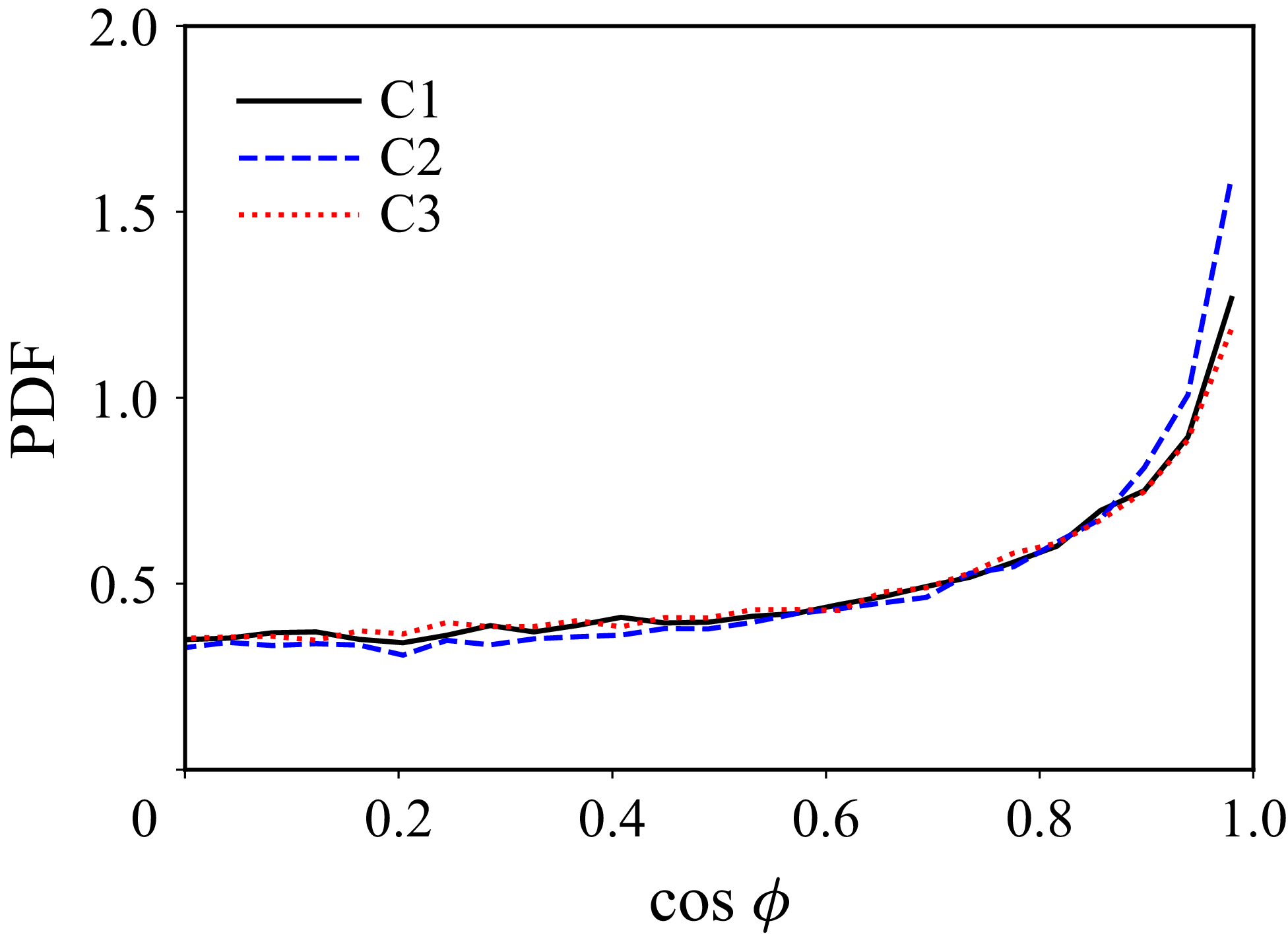
 ζ
 ω

 ς^IBBM

 Ψ
 δ

 Ψ
 aii

 Ψ
 I1
 I3

 ΨIBBM

 cosΞ,cosθ,cosη

 cosϕ

 Ψ

 Ψ
 I1−I3


 q
 r

 ⟨ωi′ωi′⟩/⟨ωi′ωi′⟩0

 ⟨θi′θi′⟩/⟨ωi′ωi′⟩

 (⟨θi′θi′⟩/⟨ωi′ωi′⟩Mm2)


 θ′2/ω0′2

 ω′2/ω0′2

 Θij
 Pij
 Mt=1.2

 Λij
 Pij
 Mt=1.2

 Open access

