1. Introduction
In [Reference Feichtner and YuzvinskyFY04], Feichtner and Yuzvinsky defined algebras
 $\mathrm{FY}({\mathcal{L}}, {\mathcal{G}})$
for every pair consisting of a geometric lattice
 $\mathcal{L}$
and a building set
 ${\mathcal{G}} \subset {\mathcal{L}}$
(such datum
 $({\mathcal{L}}, {\mathcal{G}})$
will be called a built lattice). In the realizable case over
 $\mathbb{C}$
, that is, when the geometric lattice encodes the linear dependencies of a collection of hyperplanes in a complex vector space, those algebras are the cohomology rings of the wonderful compactifications introduced by De Concini and Procesi [Reference De Concini and ProcesiDCP95]. If
 $\mathcal{G}$
is equal to
 ${\mathcal{L}}\setminus \{{\hat {0}}\}$
we get the so-called combinatorial Chow ring of
 $\mathcal{L}$
. Those rings are known to satisfy very strong properties such as Poincaré duality or even the Kähler package (see Adiprasito, Huh and Katz [Reference Adiprasito, Huh and KatzAHK18] for combinatorial Chow rings and Pagaria and Pezzoli [Reference Pagaria and PezzoliPP21] for general Feichtner–Yuzvinsky rings).
An important property of algebras which is still a largely open question for Feichtner–Yuzvinsky algebras is that of Koszulness. In plain English, Koszulness means that the algebra in question has a weight grading such that the algebra is generated by elements of weight 1, the relations between elements of weight 1 are generated by elements of weight 2 (i.e. the algebra is quadratic), the relations between elements of weight 2 are generated by elements of weight 3, and so on. Koszulness is a particularly interesting property to ask of the rational cohomology algebra of a formal space. Indeed, for those spaces we know a priori that every rational homotopy invariant can be recovered from the rational cohomology algebra, but in practice this recovery usually comes at the cost of involved computations. In contrast, when the rational cohomology algebra is Koszul, the homotopy Lie algebra, for instance, can be explicitly described as the (Lie) Koszul dual of the rational cohomology algebra (see Berglund [Reference BerglundBer14]). Since the wonderful compactifications of hyperplane arrangements are known to be formal, it is natural to ask which Feichtner–Yuzvinsky algebras are Koszul, a question raised by Dotsenko in [Reference DotsenkoDot22].
A classical approach to proving that an algebra is Koszul is to find a quadratic Gröbner basis for this algebra. Feichtner and Yuzvinsky computed explicit Gröbner bases for the Feichtner–Yuzvinsky rings, but those Gröbner bases are almost never quadratic. In fact, the Feichtner–Yuzvinsky rings themselves are not necessarily quadratic. One of the first results proving the Koszulness of certain Feichtner–Yuzvinsky algebras was provided by Dotsenko, who showed that the Feichtner–Yuzvinsky algebras associated to the complete graphs with minimal building sets are Koszul. In essence, Dotsenko defined an explicit ordering on the generators of these rings and then used the operadic structure on this collection of rings to construct a bijection between the algebraic normal monomials relative to this order and the set of quadratic relations, and the operadic normal monomials obtained in earlier work via Gröbner bases for operads (Dotsenko and Khoroshkin [Reference Dotsenko and KhoroshkinDK10]). By a dimension argument this implies that the quadratic relations form a Gröbner basis of the Feichtner–Yuzvinsky rings under consideration. More recently, Mastroeni and McCullough [Reference Mastroeni and McCulloughMM22] proved that the combinatorial Chow rings are all Koszul, using the notion of Koszul filtrations.
In [Reference StanleySta72], Stanley introduced the notion of a supersolvable lattice.
Definition 1.1 (Stanley [Reference StanleySta72]). A geometric lattice
 $\mathcal{L}$
is called supersolvable if it admits a maximal chain of modular elements.
Supersolvable geometric lattices have very nice properties in general. For instance, we have the following well-known result regarding another algebraic invariant of geometric lattices called the Orlik–Solomon algebra (which is isomorphic to the cohomology algebra of the arrangement complement in the realizable case over
 $\mathbb{C}$
).
Theorem 1.2 (Yuzvinsky [Reference YuzvinskiĭYuz01]). The Orlik–Solomon algebra of a supersolvable geometric lattice admits a quadratic Gröbner basis.
In this article we prove a similar result for Feichtner–Yuzvinsky algebras. We first introduce the notion of supersolvability for built lattices (which coincides with the usual supersolvability when considering the maximal building set) and we prove the following theorem.
Theorem 1.3.
Let
 $({\mathcal{L}}, {\mathcal{G}})$
be a supersolvable built lattice. The algebra
 $\mathrm{FY}({\mathcal{L}}, {\mathcal{G}})$
admits a quadratic Gröbner basis.
In order to prove this result we will generalize the strategy of Dotsenko by using the extended operadic structure introduced in [Reference CoronCor22]. Theorem1.3 immediately implies that combinatorial Chow rings of supersolvable geometric lattices have quadratic Gröbner bases, strengthening the result of Mastroeni and McCullough in the supersolvable case. Turning our attention towards minimal building sets, Theorem1.3 also gives us the following result.
Theorem 1.4.
Let
 $\mathcal{L}$
be a supersolvable geometric lattice and
 ${\mathcal{G}}_{\min }$
be the building set of irreducible elements of
 $\mathcal{L}$
. The algebra
 $\mathrm{FY}({\mathcal{L}}, {\mathcal{G}}_{\min })$
admits a quadratic Gröbner basis.
Stanley [Reference StanleySta72] proved that if
 ${\mathcal{L}}_{\Gamma }$
is the geometric lattice associated to a graph
 $\Gamma$
, then
 ${\mathcal{L}}_{\Gamma }$
is supersolvable whenever
 $\Gamma$
is chordal, meaning every cycle of length greater than three in
 $\Gamma$
has a chord. A refinement of that result is that if
 ${\mathcal{G}}_{\Gamma }$
is the building set of connected closed subgraphs of
 $\Gamma$
(usually called the graphical building set of
 $\Gamma$
), then the built lattice
 $({\mathcal{L}}_\Gamma , {\mathcal{G}}_\Gamma )$
is supersolvable whenever
 $\Gamma$
is chordal and connected. By Theorem1.3, this implies that the Feichtner–Yuzvinsky algebras associated to such built lattices admit a quadratic Gröbner basis. Since the complete graphs are chordal, and the graphical building sets of complete graphs coincide with the minimal building sets, we recover the result of Dotsenko.
In [Reference Losev and ManinLM00], Losev and Manin introduced moduli spaces of stable curves with marked points of two types, where the points of the first type are not allowed to coincide with any other points, and those of the second type are allowed to coincide between them. Those moduli spaces form the components of an object called the ‘extended modular operad’, introduced by Losev and Manin in the sequel [Reference Losev and ManinLM04]. In [Reference ManinMan04], Manin asked if the cohomology algebras of those moduli spaces are Koszul. Those moduli problems are governed by the graphs
 $\Gamma _{m,n}$
, where
 $\Gamma _{m,n}$
has
 $m+n$
vertices, the first
 $m$
vertices are neighbors of every vertex and the last
 $n$
vertices are neighbors only of the first
 $m$
vertices. Those graphs are chordal, which implies the following result.
Theorem 1.5.
The cohomology algebras of the components of the extended modular operad in genus
 $0$
have quadratic Gröbner bases and are therefore Koszul.
The article is organized as follows. In § 2 we introduce the combinatorial objects needed to understand the rest of the article and we recall some of their known properties. In § 3 we prove Theorem1.3 and deduce Theorem1.4. In § 4 we focus on supersolvable built lattices associated to chordal graphs, which leads to Theorem1.5. Finally, in § 5 we take a step back and give some general comments on potential topics for further research.
2. Preliminaries
In this section we introduce the main combinatorial objects that will be used throughout this paper.
2.1 Geometric lattices and matroids
Definition 2.1 (Lattice). A finite poset
 $\mathcal{L}$
is called a lattice if every pair of elements in
 $\mathcal{L}$
admits a supremum and an infimum.
The supremum of two elements
 $F_1, F_2$
is denoted by
 $F_1 \vee F_2$
and is called their join, while their infimum is denoted by
 $F_1 \wedge F_2$
and is called their meet.
Remark 2.2. Since
 $\mathcal{L}$
is supposed to be finite, having suprema and infima for pairs of elements implies having suprema and infima for any subset
 $S$
of
 $\mathcal{L}$
, which will be denoted by
 $\bigvee S$
and
 $\bigwedge S$
, respectively. As a consequence, every lattice admits an upper bound (the supremum of
 $S = {\mathcal{L}}$
) and a lower bound (the infimum of
 $S = {\mathcal{L}}$
), which will be denoted by
 $\hat {1}$
and
 $\hat {0}$
, respectively.
Definition 2.3 (Geometric lattice). A finite lattice
 $({\mathcal{L}}, \leq )$
is said to be geometric if it satisfies the following properties.
-
(i) For every pair of elements
 $F_1 \leq F_2$
, all the maximal chains of elements between
$F_1$
and
$F_2$
have the same length (Jordan–Hölder property).
-
(ii) The rank function
$\rho : {\mathcal{L}} \rightarrow \mathbb{N}$
that assigns to any element
$F$
of
$\mathcal{L}$
the length of any maximal chain of elements from
$\hat {0}$
to
$F$
satisfies the inequalityfor every
\begin{align*} \rho (F_1 \wedge F_2) + \rho (F_1 \vee F_2) \leq \rho (F_1) + \rho (F_2) \end{align*}
$F_1$
,
$F_2$
in
$\mathcal{L}$
(Sub-modularity).
-
(iii) Every element in
$\mathcal{L}$
can be obtained as the supremum of some set of atoms (i.e. elements of rank
$1$
) (Atomicity).


For any geometric lattice
 $\mathcal{L}$
we will denote by
 $\mathrm{At}({\mathcal{L}})$
its set of atoms. For any element
 $F$
in
 $\mathcal{L}$
we will denote by
 $\mathrm{At}_{\leq }(F)$
the set of atoms of
 $\mathcal{L}$
that are below
 $F$
. Elements of
 $\mathcal{L}$
of rank
 ${\mathrm{rk}} \, {\mathcal{L}} - 1$
will be called coatoms.
One of the reasons to focus on this particular class of posets comes from the study of geometric objects called hyperplane arrangements. A hyperplane arrangement
 $\mathcal{H}$
is a finite collection of hyperplanes in a finite-dimensional vector space. The set of all possible intersections of the hyperplanes of
 $\mathcal{H}$
, called the flats of
 $\mathcal{H}$
, can be ordered by reverse inclusion. The key point is that this poset, called the intersection lattice of
 $\mathcal{H}$
and denoted by
 ${\mathcal{L}}_{{\mathcal{H}}}$
, is a geometric lattice. The join in
 ${\mathcal{L}}_{{\mathcal{H}}}$
is given by the intersection of subspaces. The Jordan–Hölder property comes from the notion of dimension in linear algebra, while sub-modularity comes from the classical identity
 \begin{align*} \dim E + F = \dim E + \dim F - \dim E \cap F, \end{align*}
and atomicity is inherent in the definition of the intersection lattice. One may think of geometric lattices as a combinatorial abstraction of hyperplane arrangements. In addition, this object is equivalent to the datum of a simple loopless matroid, and therefore it has connections to many other areas in mathematics (graph theory for instance). Let us describe in more detail the correspondence between simple loopless matroids and geometric lattices. There are several equivalent definitions of matroids. We refer to [Reference WelshWel76] for more details.
Definition 2.4 (Matroids via independent subsets). A matroid is a pair comprising a finite set
 $E$
and a set
 $\mathcal{I}$
of subsets of
 $E$
(the ‘independent’ subsets) satisfying the following axioms.
-
– The set
$\mathcal{I}$
contains the empty subset. -
– For any
$I$
in
$\mathcal{I}$
, every subset of
$I$
belongs to
$\mathcal{I}$
. -
– For any
$I$
,
$J$
in
$\mathcal{I}$
, if
$\#J \gt \#I$
there exists an element
$j$
in
$J$
and not in
$I$
such that
$I \cup \{j\}$
is in
$\mathcal{I}$
.


Definition 2.5 (Matroids via closure operator). A matroid is a pair comprising a finite set
 $E$
and a map (the ‘closure operator’)
 \begin{align*} \sigma : \mathcal{P}(E) \longrightarrow \mathcal{P}(E) \end{align*}
satisfying the following axioms.
-
– For any
$X \in \mathcal{P}(E)$
we have
$X \subseteq \sigma (X)$
. -
– For any
$X \subseteq Y \in \mathcal{P}(E)$
we have
$\sigma (X) \subseteq \sigma (Y)$
. -
– For any
$X \in \mathcal{P}(E)$
we have
$\sigma (\sigma (X)) = \sigma (X)$
. -
– For any
$X \in \mathcal{P}(E)$
and
$a, b \in E$
, if
$a \in \sigma (X \cup \{b\}) \setminus \sigma (X)$
then
$b \in \sigma (X \cup \{a\}) \setminus \sigma (X)$
.






Definition 2.6 (Matroids via circuits). A matroid is a pair comprising a finite set
 $E$
and a set
 $\mathcal{C}$
of subsets of
 $E$
(the ‘circuits’) satisfying the following axioms.
-
– The empty set is not a circuit.
-
– If
$C_1 \subseteq C_2 \in {\mathcal{C}}$
then
$C_1 = C_2$
. -
– If
$C_1, C_2 \in {\mathcal{C}}$
,
$C_1 \neq C_2$
and
$e \in C_1 \cap C_2$
, then there exists a circuit
$C \subseteq C_1 \cup C_2\setminus \{e\}$
.


One can replace the last axiom by the following stronger version which we will use later in this article:
 \begin{align} &\textrm {If}\ C_1, C_2 \in {\mathcal{C}}, \, e \in C_1 \cap C_2, \, f \in C_1 \setminus C_2,\nonumber \\ & \quad \textrm{then there exists a circuit}\ C \subseteq C_1 \cup C_2 \setminus \{e\} \textrm { containing } f. \end{align}
One passes from the definition in terms of independent subsets to the definition in terms of circuits by defining a circuit as an element of
 $\mathcal{P}(E) \setminus {\mathcal{I}}$
(the ‘dependent’ subsets) that is minimal for the inclusion. One passes from the circuit definition to the closure definition by putting
 \begin{equation} \sigma (X) := X \cup \{x \, | \, \exists C \in {\mathcal{C}} \textrm { with } C \subseteq X \cup \{x\} \textrm { and } x\in C\}. \end{equation}
A matroid
 $(E, {\mathcal{I}})$
is said to be simple loopless if every subset of
 $E$
of cardinality less than or equal to two is independent. A flat of a matroid
 $(E, \sigma )$
is a subset
 $F \subseteq E$
which is closed, meaning that we have
 $\sigma (F) = F$
. The set of flats of a matroid
 $\mathrm{M}$
ordered by inclusion, denoted by
 ${\mathcal{L}}_{\mathrm{M}}$
, is a geometric lattice with meet given by the intersection. Conversely, if
 $\mathcal{L}$
is a geometric lattice then the datum
 $(E, \sigma )$
where
 $E$
is the set of atoms of
 $\mathcal{L}$
and
 $\sigma$
is the map defined by
 \begin{align*} \sigma (X) = \bigcap _{\substack {F \in {\mathcal{L}} \\ X \subset \mathrm{At}_{\leq }(F)}} \mathrm{At}_{\leq }(F) \end{align*}
is a simple loopless matroid. Those two constructions are inverse to each other on simple loopless matroids. In what follows we will freely identify an element of some geometric lattice with the set of atoms below this element. For instance, if
 $F_1$
and
 $F_2$
are two elements of some geometric lattice
 $\mathcal{L}$
then
 $F_1 \cup F_2$
will mean
 $\mathrm{At}_{\leq }({F_1}) \cup \mathrm{At}_{\leq }({F_2})$
. Finally, notice that, by definition, for any subset
 $S \subseteq {\mathcal{L}}$
with
 $\mathcal{L}$
some geometric lattice we have
 \begin{equation} \bigvee S = \sigma \biggl(\bigcup _{{F} \in S} {F}\biggr), \end{equation}
where
 $\sigma$
is the closure operator of the associated matroid. Example 2.7 provides a list of some classical geometric lattices.
Example 2.7.
-
– If
$E$
is any finite set, the set
$\mathcal{P}({E})$
of subsets of
$E$
ordered by inclusion is a geometric lattice with join the union and meet the intersection. It is the intersection lattice of the hyperplane arrangement of coordinate hyperplanes in
$\mathbb{C}^{{E}}$
. These geometric lattices are called boolean lattices and will be denoted by
$\mathcal{B}_{{E}}$
. -
– If
$V$
is any finite set, the set
$\Pi _{V}$
of partitions of
$V$
ordered by refinement is a geometric lattice. It is the intersection lattice of the so-called braid arrangement that consists of the diagonal hyperplanes
$\{z_i = z_j\}$
in
$\mathbb{C}^{{V}}$
. These geometric lattices are called partition lattices. -
– If
$\Gamma$
is any graph, one can construct the graphical matroid
$\mathrm{M}_{{\Gamma }}$
associated to
$\Gamma$
and then consider
${\mathcal{L}}_{{\Gamma }}$
the lattice of flats associated to
$\mathrm{M}_{{\Gamma }}$
(see [Reference WelshWel76] for the details of this construction). These lattices are said to be graphical. This family of geometric lattices contains the two previous examples because
$\mathcal{B}_{E}$
is the lattice associated to any tree with edge set
$E$
and
$\Pi _{V}$
is the lattice associated to the complete graph with vertex set
$V$
. For any graph
$\Gamma$
with edge set
$E$
and vertex set
$V$
, the geometric lattice
${\mathcal{L}}_{{\Gamma }}$
is the intersection lattice of the hyperplane arrangement
$\{\{z_{u} = z_{v}\}, (u,v) \in E\}$
in
$\mathbb{C}^{V}$
.


A fundamental fact about geometric lattices is that an interval of a geometric lattice is a geometric lattice (see [Reference WelshWel76]). In the rest of this article every lattice will be assumed to be geometric.
2.2 Building sets and nested sets
The following definition is due to De Concini and Procesi [Reference De Concini and ProcesiDCP95] in the realizable case, and Feichtner and Kozlov [Reference Feichtner and KozlovFK04] in general.
Definition 2.8 (Building set). Let
 $\mathcal{L}$
be a geometric lattice. A building set
 $\mathcal{G}$
of
 $\mathcal{L}$
is a subset of
 ${\mathcal{L}} \setminus \{{\hat {0}}\}$
such that for every element
 $F$
of
 $\mathcal{L}$
the morphism of posets
 \begin{equation} \prod _{G \in \max {\mathcal{G}}_{\leq {F}}}[{\hat {0}}, G] \xrightarrow {\vee } [{\hat {0}}, {F}] \end{equation}
is an isomorphism (where
 $\max {\mathcal{G}}_{\leq {F}}$
is the set of maximal elements of
 ${\mathcal{G}} \cap [{\hat {0}},{F}]$
).
The elements of
 $\max {\mathcal{G}}_{\leq {F}}$
are called the factors of
 $F$
in
 $\mathcal{G}$
.
Definition 2.9 (Built lattice). The datum of a lattice
 $\mathcal{L}$
and a building set
 $\mathcal{G}$
of
 $\mathcal{L}$
will be called a built lattice.
The definition of a building set makes sense for a larger class of posets, as shown in [Reference Feichtner and KozlovFK04], but in this paper we will restrict ourselves to the case of geometric lattices. In this particular context, building sets are geometrically motivated by the construction of wonderful compactifications for hyperplane arrangement complements. To put it simply, building sets are sets of flats of a hyperplane arrangement that one can successively blow up in order to obtain a wonderful compactification of its complement (see [Reference De Concini and ProcesiDCP95] for more details). Each blowup creates a new exceptional divisor, so that the wonderful compactification is equipped with a family of irreducible divisors indexed by
 $\mathcal{G}$
. This family of divisors forms a normal crossing divisor when
 $\mathcal{G}$
is a building set. There are a few key examples to keep in mind.
Example 2.10.
-
– Trivially, every lattice
$\mathcal{L}$
admits
${\mathcal{L}}\setminus \{{\hat {0}}\}$
as a building set. -
– Less trivially, every lattice
$\mathcal{L}$
also admits a unique minimal building set which consists of all the elements
$F$
of
$\mathcal{L}$
such that
$[{\hat {0}},F]$
is not a product of proper subposets. -
– From the definition, one can see that a building set of some lattice
$\mathcal{L}$
must contain all the atoms of
$\mathcal{L}$
. If
$\mathcal{L}$
is a boolean lattice (see Example 2.7) then its set of atoms is a building set. This fact characterizes boolean lattices. -
– If
$\mathcal{L}$
is the lattice of partitions of some finite set (see Example 2.7) then the subset of partitions with only one block having more than two elements is a building set of
$\mathcal{L}$
. This is the minimal building set of
$\mathcal{L}$
. -
– If
$\Gamma$
is a graph with graphical lattice
${\mathcal{L}}_{\Gamma }$
(see Example 2.7), then the set of elements of
${\mathcal{L}}_{\Gamma }$
corresponding to sets of edges which are connected forms a building set of
${\mathcal{L}}_{\Gamma }$
, called the graphical building set of
$\Gamma$
and denoted by
${\mathcal{G}}_{\Gamma }$
. This family of examples contains the two previous examples (by considering graphs consisting of disconnected edges for the former and complete graphs for the latter). For those two examples the graphical building set of
$\Gamma$
coincides with the minimal building set of
${\mathcal{L}}_{\Gamma }$
, but in general those two building sets can be different. For instance, for a star-shaped graph every subset of edges is connected and so in that case the graphical building set coincides with the maximal building set. In general, the minimal building set of a graphical lattice is the set of flats that form a
$2$
-connected graph. -
– Alternatively, if
$\Gamma$
is a graph with vertex set
$V$
, one can consider the boolean lattice
${\mathcal{B}}_{V}$
. This lattice has a building set made up of the ‘tubes’ of
$\Gamma$
, that is, sets of vertices of
$\Gamma$
such that the induced subgraph on those vertices is connected. This leads to the notion of graph-associahedra introduced in [Reference Carr and DevadossCD06].


A key fact about building sets is that any interval in some built lattice
 $({\mathcal{L}}, {\mathcal{G}})$
admits an ‘induced’ building set which we describe now. We start by introducing a useful notation.
Notation 2.11. For any element
 $F$
of some lattice
 $\mathcal{L}$
and a subset
 $S$
of
 $\mathcal{L}$
, we denote by
 $F\vee S$
the set of elements of
 $\mathcal{L}$
which can be obtained as the join of
 $F$
and some element of
 $S$
.
Definition 2.12 (Induced building set). Let
 $F_1 \lt F_2$
be two elements in some lattice
 $\mathcal{L}$
, with building set
 $\mathcal{G}$
. We denote by
 $\mathrm{Ind}_{[F_1, F_2]}({\mathcal{G}})$
the set
 $(F_1\vee {\mathcal{G}}) \cap (F_1, F_2]$
and we call it the induced building set on
 $[F_1, F_2]$
.
Lemma 2.13 [Reference Bibby, Denham and FeichtnerBDF21, Lemma 2.8.5]. The set
 $\mathrm{Ind}_{[F_1, F_2]}({\mathcal{G}})$
is a building set of
 $[F_1, F_2]$
.
We will write
 $\mathrm{Ind}({\mathcal{G}})$
instead of
 $\mathrm{Ind}_{[F_1, F_2]}({\mathcal{G}})$
if the interval can be deduced from the context.
Definition 2.14 (Nested set). Let
 $({\mathcal{L}}, {\mathcal{G}})$
be a built lattice. A subset
 $\mathcal{S}$
of
 $\mathcal{G}$
is called a nested set if for every subset
 ${\mathcal{A}} \subset {\mathcal{S}}$
of pairwise incomparable elements such that
 $\mathcal{A}$
has at least two elements, the join of the elements of
 $\mathcal{A}$
does not belong to
 $\mathcal{G}$
. The nested sets of a built lattice
 $({\mathcal{L}}, {\mathcal{G}})$
form an abstract simplicial complex denoted
 ${\mathcal{N}}({\mathcal{L}},{\mathcal{G}})$
. We denote by
 ${\mathcal{N}}^{\mathrm{irr}}({\mathcal{L}}, {\mathcal{G}})$
the set of nested sets of
 $({\mathcal{L}}, {\mathcal{G}})$
containing the maximal elements of
 $\mathcal{G}$
.
Example 2.15. A chain of elements in some building set
 $\mathcal{G}$
is always nested and those are the only nested sets of the maximal building set
 ${(\mathcal{G}} = {\mathcal{L}} \setminus \{{\hat {0}} \})$
.
Geometrically, nested sets correspond to sets of divisors in the wonderful compactification which have a nontrivial intersection. Those intersections form a stratification of the wonderful compactification. If the building set
 $\mathcal{G}$
contains the maximal element
 $\hat {1}$
, the wonderful compactification of the projectivized hyperplane arrangement complement can be identified with the proper transform of the exceptional divisor created after blowing up
 $\hat {1}$
in the wonderful compactification of the linear arrangement complement. Under this identification the nested sets
 ${\mathcal{N}}^{\mathrm{irr}}({\mathcal{L}}, {\mathcal{G}})$
index the strata of the wonderful compactification of the projectivized arrangement complement.
2.3 Supersolvable built lattices
Recall that an element
 $F$
in some geometric lattice
 $\mathcal{L}$
is called modular if for every pair of elements
 $F_1,F_2 \in {\mathcal{L}}$
such that
 $F_2 \leq F$
, one has the equality
 \begin{align*} F\wedge (F_1 \vee F_2) = (F\wedge F_1) \vee F_2, \end{align*}
or, equivalently, if for every pair of elements
 $F_1, F_2 \in {\mathcal{L}}$
such that
 $F_2 \leq F_1$
, one has the equality
 \begin{align*} F_1\wedge (F \vee F_2) = (F\wedge F_1) \vee F_2. \end{align*}
The equivalence between those two definitions is a consequence of geometricity (see [Reference BirkhoffBir40, p. 83]). The following definition is due to Stanley [Reference StanleySta72].
Definition 2.16 (Supersolvable lattice). A geometric lattice
 $\mathcal{L}$
is said to be supersolvable if it has a maximal chain of modular elements.
Let
 $\mathcal{H}$
be some hyperplane arrangement with total intersection
 $\{0\}$
in some complex vector space
 $V$
. In this setting, a modular coatom
 $L$
in the intersection lattice of
 $\mathcal{H}$
corresponds to a line such that the projection
 $V \rightarrow V/L$
induces a fibration between the arrangement complement of
 $\mathcal{H}$
and the arrangement complement of the contraction
 ${\mathcal{H}} /L$
(the collection of hyperplanes of
 $\mathcal{H}$
containing
 $L$
viewed in
 $V/L$
). A supersolvable arrangement is an arrangement whose complement admits a chain of fibrations of the above form, with final term
 $\mathbb{C}^{\star }$
. We refer to Orlik and Terao [Reference Orlik and TeraoOT91] for more details.
Fact 2.17. Supersolvability is a hereditary condition (meaning it is stable by taking intervals) because if
 $F$
is some element in some supersolvable lattice
 $\mathcal{L}$
with chain of modular elements
 \begin{align*} {\hat {0}} = F_1 \lt \cdots \lt F_n = \hat {1}, \end{align*}
then the chains
 \begin{align*} F_1\wedge F \leq \cdots \leq F_n \wedge F \end{align*}
and
 \begin{align*} F_1 \vee F \leq \cdots \leq F_n \vee F \end{align*}
are maximal chains (with possibly multiple occurrences) consisting of modular elements of
 $[{\hat {0}}, F]$
and
 $[F, \hat {1}]$
, respectively (see [Reference StanleySta72, Proposition 3.2 and proof of Theorem1.2]).
Our first goal in this paper is to define a suitable notion of supersolvability for built lattices
 $({\mathcal{L}}, {\mathcal{G}})$
instead of lattices. It is natural to ask for the maximal chain of modular elements to belong to
 $\mathcal{G}$
rather than just
 $\mathcal{L}$
. However, if we stop here then our notion is not hereditary because the meets
 $G_i \wedge G$
(with
 $G_i$
some element in the maximal chain and
 $G$
in
 $\mathcal{G}$
) have no reason to belong to
 $\mathrm{Ind}_{[{\hat {0}}, G]}({\mathcal{G}})$
. On the other hand, we notice that the joins
 $G_i \vee G$
do belong to
 $\mathrm{Ind}_{[G, \hat {1}]}({\mathcal{G}})$
, by definition of the induced building set. This motivates the following definition.
Definition 2.18 (Supersolvable built lattice). A built lattice
 $({\mathcal{L}}, {\mathcal{G}})$
is said to be supersolvable if it admits a maximal chain
 ${\hat {0}} = G_1 \lt \cdots \lt G_n = \hat {1}$
consisting of modular elements belonging to
 $\mathcal{G}$
such that for any element
 $G$
in
 $\mathcal{G}$
, the element
 $G_i \wedge G$
belongs to
 ${\mathcal{G}} \cup \{{\hat {0}}\}$
for all
 $i\leq n$
.
As a first remark, notice that if
 $({\mathcal{L}}, {\mathcal{G}})$
is a supersolvable built lattice then
 $\mathcal{L}$
is supersolvable (using the same maximal chain). On the other hand if a lattice
 $\mathcal{L}$
is supersolvable then the built lattice
 $({\mathcal{L}}, {\mathcal{G}}_{\max })$
is a supersolvable built lattice. In §§ 3 and 4 we will introduce other large classes of supersolvable built lattices. For now, let us consider the following simple example.
Example 2.19. Let
 ${\mathcal{B}}_{4}$
be the boolean lattice on
 $\{1, 2, 3 ,4\}$
. If we put
 \begin{align*} {\mathcal{G}} := \{\{1\}, \{2\}, \{3\}, \{4\}, \{1,2\}, \{1,2,3\}, \{1,2,3,4\}, \{2,3,4\}, \{2,3\}\}, \end{align*}
then the built lattice
 $({\mathcal{B}}_{4}, {\mathcal{G}})$
is supersolvable. Indeed, the chain
 \begin{align*} \{1\}\subset \{1, 2\} \subset \{1, 2 ,3\} \subset \{1, 2, 3, 4\} \end{align*}
is a maximal chain of modular elements in
 $\mathcal{G}$
(all the elements of
 ${\mathcal{B}}_4$
are modular), and we have
 \begin{align*} \{2,3,4\}\wedge \{1,2,3\} = \{2, 3\} \in {\mathcal{G}}. \end{align*}
On the contrary, if one puts
 ${\mathcal{G}}' := {\mathcal{G}} \setminus \{2, 3\} \cup \{3,4\}$
then
 $({\mathcal{B}}_4, {\mathcal{G}}')$
is not a supersolvable built lattice because we have
 \begin{align*} \{1,2,3\} \wedge \{2, 3, 4\} = \{2, 3\}\notin {{\mathcal{G}}'}, \end{align*}
and any maximal chain of elements in
 ${\mathcal{G}}'$
must contain either
 $\{1, 2 ,3\}$
or
 $\{2, 3,4\}$
.
Example 2.20. For a general boolean matroid
 ${\mathcal{B}}_E$
with
 $E$
some finite set, since every element in a boolean matroid is modular, choosing a maximal chain of modular elements
 \begin{align*} \emptyset \subset \{e_1\} \subset \{e_1, e_2\} \subset \cdots \end{align*}
in
 ${\mathcal{B}}_E$
is the same as choosing a total order
 $e_1 \vartriangleleft e_2 \vartriangleleft \cdots$
on
 $E$
. For any building set
 $\mathcal{G}$
of
 ${\mathcal{B}}_E$
, the built lattice
 $({\mathcal{B}}_E, {\mathcal{G}})$
is supersolvable with maximal chain specified by
 $\vartriangleleft$
if and only if for all
 $G \in {\mathcal{G}}$
and
 $e\in E$
we have that
 $E_{\trianglelefteq e} \wedge G \, (= G_{\trianglelefteq e})$
belongs to
 ${\mathcal{G}}\cup \{\emptyset \}$
. This recovers the notion of a chordal building set introduced in [Reference Postnikov, Reiner and WilliamsPRW08].
One has the following analog of Fact 2.17 for built lattices.
Lemma 2.21.
Let
 $({\mathcal{L}}, {\mathcal{G}})$
be a supersolvable built lattice. For any
 $F\leq G \in {\mathcal{L}}$
, if
 $G$
belongs to
 $\mathcal{G}$
then the built lattice
 $([F, G], \mathrm{Ind}_{[F,G]}({\mathcal{G}}))$
is supersolvable.
Proof.
Let us denote by
 $(G_i)_i$
a maximal chain witnessing the supersolvability of
 $({\mathcal{L}}, {\mathcal{G}})$
. It is enough to prove the lemma for
 $F={\hat {0}}$
or
 $G = \hat {1}$
. For
 $F = {\hat {0}}$
, by Fact 2.17 and the definition of
 $(G_i)_i$
one has that the chain
 $(G_i\wedge G)_i$
is a maximal chain in
 $[{\hat {0}},G]$
consisting of modular elements of
 $[{\hat {0}},G]$
belonging to
 $\mathrm{Ind}_{[{\hat {0}},G]}({\mathcal{G}}) = {\mathcal{G}}\cap [{\hat {0}}, G]$
. Furthermore, for any element
 $G'$
in
 $\mathrm{Ind}_{[{\hat {0}},G]}({\mathcal{G}})$
and any
 $i$
we have
 \begin{align*} (G_i\wedge G)\wedge G' = G_i \wedge G' \in \mathrm{Ind}_{[{\hat {0}},G]}({\mathcal{G}}), \end{align*}
again by the definition of
 $(G_i)_i$
. Let us now assume that we have
 $G = \hat {1}$
. Let
 $(G'_j)_j$
be the factors of
 $F$
in
 $\mathcal{G}$
. By successively restricting to
 $[G'_1, \hat {1}], [G'_1 \vee G'_2, \hat {1}], \ldots , [F = \bigvee _j G'_j, \hat {1}]$
one can further assume that
 $F$
belongs to
 $\mathcal{G}$
. By Fact 2.17 and the definition of
 $\mathrm{Ind}_{[F, \hat {1}]}({\mathcal{G}})$
the chain
 $(G_i\vee F)_i$
is maximal in
 $[F, \hat {1}]$
and consists of modular elements of
 $[F, \hat {1}]$
in
 $\mathrm{Ind}_{[F, \hat {1}]}({\mathcal{G}})$
. What is left to prove is that for any element
 $G\vee F$
in
 $\mathrm{Ind}_{[F, \hat {1}]}({\mathcal{G}})$
and any
 $i$
the element
 $(G_i \vee F)\wedge (G\vee F)$
belongs to
 $\mathrm{Ind}_{[F, \hat {1}]}({\mathcal{G}})$
. By modularity of
 $G_i$
one has
 \begin{align*} (G_i \vee F)\wedge (G\vee F) = (G_i\wedge (G\vee F))\vee F. \end{align*}
Since
 $F$
was assumed to belong to
 $\mathcal{G}$
, we either have that
 $G\vee F$
belongs to
 $\mathcal{G}$
or that
 $G$
and
 $F$
are the two (distinct) factors of
 $G\vee F$
. In the first case, we immediately get that
 $(G_i\wedge (G\vee F))\vee F$
belongs to
 $\mathrm{Ind}_{[F, \hat {1}]}({\mathcal{G}})$
by the definitions of
 $(G_i)_i$
and
 $\mathrm{Ind}_{[F, \hat {1}]}({\mathcal{G}})$
. In the second case, using the isomorphism
 $[{\hat {0}}, G]\times [{\hat {0}}, F]\simeq [{\hat {0}}, G\vee F]$
one gets the identity
 \begin{align*} (G_i\wedge (G\vee F))\vee F = (G_i \wedge G) \vee F, \end{align*}
and once again by the definitions of
 $(G_i)_i$
and
 $\mathrm{Ind}_{[F, \hat {1}]}({\mathcal{G}})$
we get that
 $(G_i \vee F)\wedge (G\vee F)$
belongs to
 $\mathrm{Ind}_{[F, \hat {1}]}({\mathcal{G}})$
.
Note that for any
 $F \leq G$
with
 $G\in {\mathcal{G}}$
, by modularity of the
 $G_i$
(keeping the notations of the previous proof) we have the equality
 \begin{align*} (G_i\vee F)\wedge G = (G_i \wedge G) \vee F \end{align*}
for any
 $i$
. In other words, restricting
 $(G_i)_i$
to
 $[F, \hat {1}]$
and then to
 $[F, G]$
as in Fact 2.17, yields the same result as first restricting to
 $[{\hat {0}}, G]$
and then to
 $[F,G]$
. This means that choosing a chain witnessing the supersolvability of
 $({\mathcal{L}}, {\mathcal{G}})$
induces canonical choices of chains witnessing the supersolvability of
 $[F,G]$
for any
 $F \leq G$
, with
 $G\in {\mathcal{G}}$
.
Definition 2.22 (Initial segment). For any supersolvable built lattice
 $({\mathcal{L}},{\mathcal{G}})$
with maximal chain of modular elements
 $(G_i)_i$
, and any
 $F \leq G \in {\mathcal{L}}$
with
 $G\in {\mathcal{G}}$
, we denote
 \begin{align*} F = {\mathrm{d}}^r_F(G) \lt {\mathrm{d}}^{r-1}_F(G) \lt \cdots \lt {\mathrm{d}}^1_F(G) \lt {\mathrm{d}}^0_F(G) = G \end{align*}
as the maximal chain of modular elements in
 $\mathrm{Ind}_{[F,G]}({\mathcal{G}})$
induced by
 $(G_i)_i$
(with
 $r = {\mathrm{rk}} \,G - {\mathrm{rk}} \, F$
). To be explicit,
 ${\mathrm{d}}^k_{F}(G)$
is the biggest element of the form
 $(G_i \vee F)\wedge G$
(or equivalently of the form
 $(G_i \wedge G)\vee F$
) such that
 ${\mathrm{rk}} \, G - {\mathrm{rk}} \, {\mathrm{d}}^k_{F}(G) \geq k$
. An element of the form
 ${\mathrm{d}}^k_F(G)$
which is different from
 $F$
will be called an initial segment of
 $G$
relative to
 $F$
.
If
 $F$
is equal to
 $\hat {0}$
we will omit it. In the case
 $k = 1$
we will write
 $\mathrm{d}$
instead of
 ${\mathrm{d}}^{1}$
.
Remark 2.23. The term ‘initial segment’ is motivated by the example of built lattices associated to complete graphs with the building set of connected subgraphs (see Example 2.10) studied by Dotsenko in [Reference DotsenkoDot22]. In this example, if we label the vertices of our complete graph from
 $1$
to
 $n$
, a nonempty closed connected subgraph can be uniquely described by the vertices it contains, which can be any subset of
 $\{1, \ldots , n\}$
with more than two elements. Under this identification, the building set of connected subgraphs has a maximal chain of modular elements given by
 ${\hat {0}} \leq \{1,2\} \leq \{1,2,3\} \leq \cdots \leq \{1,\ldots , n\}$
(of course any maximal chain in this building set would have done the job). For any connected closed subgraph represented by some subset
 $S = \{i_1 \lt \cdots \lt i_k\}$
, the initial segments of
 $S$
are the subsets
 $\{i_1,i_2\}, \{i_1, i_2, i_3\}, \ldots , \{i_1,\ldots , i_{k}\}$
, hence the terminology. One also has the following alternative motivation, which works for any supersolvable built lattice
 $({\mathcal{L}}, {\mathcal{G}})$
. Start by choosing any total order
 $\vartriangleleft$
on the atoms of
 $\mathcal{L}$
satisfying the property that for any atoms
 $H$
,
 $H'$
, if there exists some integer
 $k$
such that
 $H\leq {\mathrm{d}}^k(\hat {1})$
and
 $H' \nleq {\mathrm{d}}^k(\hat {1})$
then
 $H\vartriangleleft H'$
. For any
 $G\in {\mathcal{G}}$
identified with some set of atoms
 $\{H_1 \vartriangleleft \cdots \vartriangleleft H_k\}$
, the initial segments of
 $G$
are exactly the nonempty flats of the form
 $\{H_1 \vartriangleleft \cdots \vartriangleleft H_i\}$
for some
 $i\leq k$
. This is a consequence of the fact that the meet in a geometric lattice is just the intersection in terms of sets of atoms.
Example 2.24. Let
 $({\mathcal{B}}_E, {\mathcal{G}})$
be a supersolvable built lattice with supersolvable structure given by some total order on
 $E$
(see Example 2.20). For any
 $F\subset G \subset E$
with
 $G \in {\mathcal{G}}$
, the subset
 ${\mathrm{d}}_F(G)$
is
 $G \setminus \{\max (G \setminus F)\}.$
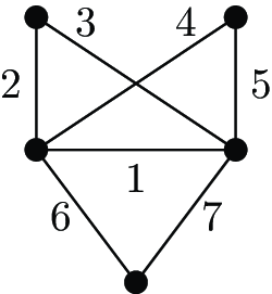
Example 2.25. Consider the graph
 $\Gamma$
of Figure 1 with edge set
 $\{1,\ldots , 7\}$
, and
 $({\mathcal{L}}_\Gamma , {\mathcal{G}}_\Gamma )$
its associated built lattice (see Example 2.10). This built lattice is supersolvable with maximal chain of modular elements
 ${\hat {0}} \lt \{1\} \lt \{1,2,3\}\lt \{1,2,3,4,5\}\lt \hat {1}$
(this will be a consequence of Lemma 4.1). The natural order on integers is a total order on the atoms of
 ${\mathcal{L}}_\Gamma$
(i.e. the edges of
 $\Gamma$
) as in the second part of Remark 2.23. The initial segments of
 $\{2, 4 ,6\} \in {\mathcal{G}}_\Gamma$
are
 $\{2\}$
,
 $\{2,4\}$
and
 $\{2,4,6\}$
. The initial segments of
 $\{1, 4 ,5, 6 ,7\} \in {\mathcal{G}}_\Gamma$
are
 $\{1\}$
,
 $\{1, 4 ,5\}$
and
 $\{1,4,5,6,7\}$
.
A graph giving a supersolvable built lattice.

Convention. In the sequel, whenever we introduce a supersolvable built lattice we implicitly choose a particular maximal chain of modular elements of this built lattice. Any interval in this built lattice is implicitly considered with its induced supersolvable structure.
To conclude this subsection we prove a small general lemma which will be useful later on.
Lemma 2.26.
Let
 $\mathcal{L}$
be a geometric lattice,
 $F$
a modular element of
 $\mathcal{L}$
and
 $C$
a circuit in
 $\mathcal{L}$
. At least one of the following propositions is true:
-
–
$C \subset F$
; -
–
$C \cap F = \emptyset$
; -
– there exists a circuit
$C'$
such that
$C'\cap F$
is a singleton
$\{H\}$
and
$C'\setminus \{H\}$
is included in
$C\setminus (F\cap C)$
.


Proof. Assume the first two propositions are not true. Let us denote
 \begin{align*} &I := C \cap F, \\ &J := C \setminus I. \end{align*}
Let
 $H$
be any element of
 $I$
, which is not empty by assumption. By modularity of
 $F$
we have
 \begin{equation} F\wedge (\sigma (I \setminus \{H\}) \vee \sigma (J)) = \sigma (I \setminus \{H\}) \vee (F\wedge \sigma (J)). \end{equation}
Since
 $C$
is a circuit we have
 $\sigma (I\setminus \{H\})\vee \sigma (J) = \sigma (C)$
, and so the element on the left of (5) must contain
 $I$
which has rank
 $\#I$
. Since
 $\sigma (I \setminus \{H\})$
only has rank
 $\#I -1$
we must have
 \begin{align*} F\wedge \sigma (J) \neq {\hat {0}}. \end{align*}
By (2), this implies that we have the desired circuit
 $C'$
.
2.4 The Feichtner–Yuzvinsky rings
Definition 2.27. For every built lattice
 $({\mathcal{L}}, {\mathcal{G}})$
we define the Feichtner–Yuzvinsky graded commutative ring
 $\mathrm{FY}({\mathcal{L}}, {\mathcal{G}})$
by
 \begin{align*} \mathrm{FY}({\mathcal{L}}, {\mathcal{G}}) = \mathbb{Z}[x_G, \,G \in {\mathcal{G}}]/ {\mathcal{I}}_{\mathrm{aff}}, \end{align*}
with all the generators in degree
 $2$
, and
 ${\mathcal{I}}_{\mathrm{aff}}$
the ideal generated by elements
 \begin{align*} \sum _{G \geq H}x_G \end{align*}
for every atom
 $H$
, and elements
 \begin{align*} \prod _{G \in S}x_G \end{align*}
for every set
 $S \subset {\mathcal{G}}$
which is not nested.
In the realizable case, the ring
 $\mathrm{FY}({\mathcal{L}}, {\mathcal{G}})$
is the cohomology ring of the wonderful compactification associated to the building set
 $\mathcal{G}$
(see [Reference De Concini and ProcesiDCP95] for the computation of the cohomology ring). Those rings were generalized to arbitrary built lattices by Feichtner and Yuzvinsky in [Reference Feichtner and YuzvinskyFY04]. The Feichtner–Yuzvinsky rings admit another important presentation, called the simplicial presentation.
Proposition 2.28 [Reference Pagaria and PezzoliPP21, Theorem 2.9]. For every built lattice
 $({\mathcal{L}}, {\mathcal{G}})$
we have the presentation
 \begin{align*} \mathrm{FY}({\mathcal{L}}, {\mathcal{G}}) \simeq \mathbb{Z}[h_G, \, G \in {\mathcal{G}}] / {\mathcal{I}}_{\mathrm{simp}} \end{align*}
where
 ${\mathcal{I}}_{\mathrm{simp}}$
is the ideal generated by relations
 \begin{align*} h_H \end{align*}
for every atom
 $H$
and
 \begin{align*} \prod _{G' \in {\mathcal{A}}} (h_G - h_{G'}) \end{align*}
for every
 $G \in {\mathcal{G}}$
and
 $\mathcal{A}$
a set of pairwise incomparable elements in
 $\mathcal{G}$
such that
 $\bigvee {\mathcal{A}}$
is equal to
 $G$
. The change of variables between the last presentation and the defining presentation is given by
 \begin{align*} h_G = \sum _{G' \geq G}x_{G'}. \end{align*}
This presentation appeared first in [Reference YuzvinskyYuz02] in the realizable case and it is extensively studied in [Reference Backman, Eur and SimpsonBES20] in the case of maximal building sets. It is widely used in [Reference Pagaria and PezzoliPP21]. In this article we will use exclusively this presentation. In [Reference Feichtner and YuzvinskyFY04], the authors address the issue of finding a Gröbner basis for
 ${\mathcal{I}}_{\mathrm{aff}}$
(see [Reference Becker and WeispfenningBW93] for a reference on Gröbner bases) and they show that, when considering any linear order on generators refining the reverse order on
 $\mathcal{G}$
and the induced degree-lexicographic ordering on monomials, although the elements defining
 ${\mathcal{I}}_{\mathrm{aff}}$
do not form a Gröbner basis in general, one can still describe a fairly manageable Gröbner basis. Recall the following key definition in Gröbner bases theory.
Definition 2.29 (Normal monomial). Let
 $\vartriangleleft$
be a total order on the monomials of
 $A := \mathbb{Z}[x_1, \ldots , x_n]$
. The leading term of a nonzero element
 $f$
in
 $A$
is the maximal nonzero term (for
 $\vartriangleleft$
) in the expansion of
 $f$
. For any subset
 $R \subset A$
, a monomial
 $m$
of
 $A$
is said to be normal with respect to
 $R$
and
 $\vartriangleleft$
if it is not divisible by the leading term of some element in
 $R$
.
Theorem 2.30 [Reference Feichtner and YuzvinskyFY04, Theorem 2]. Elements of the form
 $(\prod _{G \in {\mathcal{S}}}x_G) h_{G'}^{\rho (G') - \rho (\bigvee S)}$
with
 $\mathcal{S}$
any nested set and
 $G'$
any element of
 $\mathcal{G}$
satisfying
 $G' \gt \bigvee {\mathcal{S}}$
, together with the usual
 $\prod _{G \in S} x_G$
for every non-nested set
 $S$
, form a Gröbner basis of
 ${\mathcal{I}}_{\mathrm{aff}}$
for the degree-lexicographic order on monomials induced by any linear order on generators refining the reverse order of
 $\mathcal{L}$
. The normal monomials with respect to that Gröbner basis and that total order are monomials of the form
 \begin{align*} x_{G_1}^{\alpha _1}\cdots x_{G_n}^{\alpha _n}, \end{align*}
where the
 $G_i$
form a nested set
 $\mathcal{S}$
and for every
 $i \leq n$
we have
 $\alpha _i \lt {\mathrm{rk}} [\bigvee {\mathcal{S}}_{\lt G_i}, G_i]$
.
Those Gröbner bases are almost never quadratic. The rest of the paper will be devoted to proving the following theorem.
Theorem 2.31.
Let
 $({\mathcal{L}}, {\mathcal{G}})$
be a supersolvable built lattice. The Feichtner–Yuzvinsky ring
 $\mathrm{FY}({\mathcal{L}}, {\mathcal{G}})$
admits a quadratic Gröbner basis and is therefore Koszul.
The proof of this theorem will be carried out in §§ 3.1 and 3.2. The following proposition is a small step toward Theorem2.31 that we will need later on.
Proposition 2.32.
Let
 $({\mathcal{L}}, {\mathcal{G}})$
be a supersolvable built lattice. The Feichtner–Yuzvinsky ring
 $\mathrm{FY}({\mathcal{L}}, {\mathcal{G}})$
is quadratic.
Proof.
It is enough to prove that if
 $({\mathcal{L}}, {\mathcal{G}})$
is supersolvable then the nested set complex of
 $({\mathcal{L}}, {\mathcal{G}})$
is flag, meaning that for any pairwise incomparable elements
 $G_1, \ldots , G_n$
in
 $\mathcal{G}$
with
 $n\geq 2$
, if
 $G_1 \vee \cdots \vee G_n$
belongs to
 $\mathcal{G}$
then there exists
 $i \neq j \leq n$
such that
 $G_i \vee G_j$
belongs to
 $\mathcal{G}$
. We will prove this statement by induction on the rank of
 $\mathcal{L}$
. By restriction (Lemma 2.21) we can assume that we have
 $G_1\vee \cdots \vee G_n = \hat {1}$
. If
 $\mathcal{L}$
has rank
 $2$
, then for any
 $i\neq j$
we have
 $G_i\vee G_j = \hat {1} \in {\mathcal{G}}$
. In general, let us consider
 $i_0$
any index such that
 $G_{i_0} \nleq {\mathrm{d}}(\hat {1})$
(such an index exists as otherwise we would have
 ${\mathrm{d}}(\hat {1}) = \hat {1}$
). For any
 $j \neq i_0$
, if
 $G_{i_0} \vee G_j$
belongs to
 $\mathcal{G}$
then we are done. Otherwise the isomorphism
 $[{\hat {0}}, G_{i_0} \vee G_j]\simeq [{\hat {0}}, G_{i_0}]\times [{\hat {0}}, G_j]$
yields the identity
 \begin{align*} {\mathrm{d}}(\hat {1})\wedge (G_{i_0} \vee G_j) = ({\mathrm{d}}(\hat {1})\wedge G_{i_0}) \vee ({\mathrm{d}}(\hat {1})\wedge G_j). \end{align*}
By modularity of
 ${\mathrm{d}}(\hat {1})$
the element
 ${\mathrm{d}}(\hat {1})\wedge (G_{i_0} \vee G_j)$
is a coatom of
 $G_{i_0} \vee G_j$
(Fact 2.17). This, together with the last identity, implies that
 $G_j$
must be less than or equal to
 ${\mathrm{d}}(\hat {1})$
. This means that we have the inequality
 ${\mathrm{d}}(\hat {1}) \geq ({\mathrm{d}}(\hat {1})\wedge G_{i_0})\vee \bigvee _{j \neq i_0}G_j$
. However, again by modularity of
 ${\mathrm{d}}(\hat {1})$
, we have that
 ${\mathrm{d}}(\hat {1}) \wedge G_{i_0}$
is a coatom of
 $G_{i_0}$
. By sub-modularity of
 $\mathcal{L}$
, this implies that
 $({\mathrm{d}}(\hat {1})\wedge G_{i_0})\vee \bigvee _{j \neq i_0}G_j$
is a coatom of
 $\mathcal{L}$
and thus must be equal to
 ${\mathrm{d}}(\hat {1})$
by the previous inequality. Note that
 ${\mathrm{d}}(\hat {1})\wedge G_{i_0}$
is an element in
 ${\mathcal{G}}\cup \{{\hat {0}}\}$
by the definition of supersolvability for built lattices. The induction hypothesis on
 $[{\hat {0}}, {\mathrm{d}}(\hat {1})]$
yields that we must have
 $G_{j}\vee G_{j'} \in {\mathcal{G}}$
for some
 $j\neq j'(\neq i_0)$
, which concludes the proof.
If the element
 ${\mathrm{d}}(\hat {1})$
is not modular, there can be several indexes
 $i$
such that
 $G_i \nleq {\mathrm{d}}(\hat {1})$
, and the element
 $\bigvee _{G_i \nleq {\mathrm{d}}(\hat {1})}({\mathrm{d}}(\hat {1})\wedge G_{i})\vee \bigvee _{G_j \leq {\mathrm{d}}(\hat {1})}G_j$
can be strictly smaller than
 ${\mathrm{d}}(\hat {1})$
, which means that one cannot obtain a new family of elements having join
 ${\mathrm{d}}(\hat {1})$
with no binary join in
 $\mathcal{G}$
, as we got in the previous proof. For instance, consider the lattice associated to a
 $5$
-cycle (see Example 2.7) with edges numbered from
 $1$
to
 $5$
, together with the building set
 $\{\{1\}, \ldots , \{5\}, \{1,2\}, \{1, 2 ,3\}, \{1, 2, 3, 4, 5\}\}$
, and maximal chain of elements
 \begin{align*} {\hat {0}} \lt \{1\} \lt \{1,2\} \lt \{1,2,3\} \lt \hat {1} \end{align*}
(which are not all modular). The family
 $G_i = \{i\}, i \gt 1$
has join
 $\hat {1}$
and no binary join in
 $\mathcal{G}$
. Only
 $\{2\}$
and
 $\{3\}$
out of the four
 $G_i$
are below
 ${\mathrm{d}}(\hat {1}) = \{1, 2 ,3\}$
and the join of
 $\{2\}$
and
 $\{3\}$
is
 $\{2,3\}$
instead of
 $\{1,2,3\}$
.
2.5 The operadic structure on built lattices
In order to prove Theorem2.31 we will use the operadic structure on built lattices introduced in [Reference CoronCor22]. Let us quickly summarize this construction, referring to the latter article for more details. From now on, all nested sets are assumed to contain the maximal elements of the building set they live in.
For any built lattice
 $({\mathcal{L}}, {\mathcal{G}})$
and any nested set
 $\mathcal{S}$
in
 $\mathcal{G}$
we have maps of algebras
 \begin{equation} \begin{array}{ccc} \mathrm{FY}({\mathcal{L}}, {\mathcal{G}}) & \xrightarrow {\mathrm{FY}({\mathcal{S}})} &\bigotimes _{G \in {\mathcal{S}}}\mathrm{FY}([\bigvee {\mathcal{S}}_{\lt G}, G],\mathrm{Ind}({\mathcal{G}})), \\ h_{G'} & \longrightarrow & 1\otimes \cdots \otimes 1 \otimes h_{(\bigvee {\mathcal{S}}_{\lt G})\vee G'} \otimes 1 \otimes \cdots \otimes 1, \end{array} \end{equation}
where
 $G$
is the minimal element of
 $\mathcal{S}$
such that we have
 $G' \lt G$
. In [Reference CoronCor22] we show that the collection of Feichtner–Yuzvinsky algebras
 $\{\mathrm{FY}({\mathcal{L}}, {\mathcal{G}}), ({\mathcal{L}}, {\mathcal{G}})\}$
together with the above morphisms can be formalized as a cooperad over a certain Feynman category (Kaufmann and Ward [Reference Kaufmann and WardKW17]) denoted
 $\mathfrak{LBS}$
having as objects the built lattices and morphisms the nested sets. The key ingredient is the definition of an associative composition of nested sets: for every nested set
 ${\mathcal{S}} \in {\mathcal{N}}^{\mathrm{irr}}({\mathcal{L}}, {\mathcal{G}})$
and every collection of nested sets
 \begin{align*} \left({\mathcal{S}}_G \in {\mathcal{N}}^{\mathrm{irr}}\Big(\Big[\bigvee {\mathcal{S}}_{\lt G}, \hat {1} \Big], \mathrm{Ind}({\mathcal{G}})\Big)\right)_{G \in {\mathcal{S}}} \end{align*}
one can define
 ${\mathcal{S}}\circ ({\mathcal{S}}_{G})_{G} \in {\mathcal{N}}^{\mathrm{irr}}({\mathcal{L}}, {\mathcal{G}})$
such that the operation
 $\circ$
is associative (this is the composition of morphisms in
 $\mathfrak{LBS}$
). In the case of the maximal building set, the composition of nested sets is just the concatenation of chains.
The operad
 $\mathbb{FY}^{\vee } = \{\mathrm{FY}^{\vee }({\mathcal{L}}, {\mathcal{G}}), ({\mathcal{L}}, {\mathcal{G}})\}$
with structural morphisms given by the linear duals of morphisms (6) admits a quadratic presentation with one generator of top degree (the degree map) in each arity (each built lattice
 $({\mathcal{L}}, {\mathcal{G}})$
). The ‘monomials’ in
 $\mathbb{FY}^{\vee }$
are all possible operadic products of those generators. Since we have only one generator in each arity, the monomials living in some Feichtner–Yuzvinsky ring
 $\mathrm{FY}({\mathcal{L}}, {\mathcal{G}})$
are in bijection with the nested sets of
 $({\mathcal{L}}, {\mathcal{G}})$
. In [Reference CoronCor22, Section 5] we construct a Gröbner basis machinery for operads over
 $\mathfrak{LBS}$
via the introduction of a notion of shuffle
 $\mathfrak{LBS}$
-operads, governed by another Feynman category having as objects the directed built lattices (built lattices together with an order on the atoms of
 $\mathcal{L}$
). This machinery revolves around the following notion of operadic normal monomials, which is the analog of Definition 2.29 for operads.
Definition 2.33 (Operadic normal monomial). Let
 $\vartriangleleft$
be a total order on the monomials of some free operad
 $\mathcal{O}$
in abelian groups. The leading term of a nonzero element
 $f$
in
 $\mathcal{O}$
is the maximal nonzero term (for
 $\vartriangleleft$
) in the expansion of
 $f$
. For any set
 $R$
of elements of
 $\mathcal{O}$
, a monomial
 $m$
of
 $\mathcal{O}$
is said to be normal with respect to
 $R$
and
 $\vartriangleleft$
if it is not divisible by the leading term of some element in
 $R$
.
We refer to [Reference CoronCor22, Section 5] for more details. One can compute an (operadic) Gröbner basis for
 $\mathbb{FY}^{\vee }$
and describe the associated (operadic) normal monomials as follows. Let
 $({\mathcal{L}}, {\mathcal{G}}, \vartriangleleft )$
be a directed built lattice such that
 $\hat {1} \in {\mathcal{G}}$
. The total order on atoms
 $\vartriangleleft$
defines an EL-labeling
 $\lambda _{\vartriangleleft }$
by putting
 \begin{align*} \lambda _{\vartriangleleft }(F_1\prec F_2) = \min \,\{H \in \mathrm{At}({\mathcal{L}}) \, | \, F_1 \vee H = F_2\}. \end{align*}
We refer to [Reference WachsWac06] for a reference on EL-labelings. For any two elements
 $F_1\lt F_2$
in
 $\mathcal{L}$
and
 $k$
some positive integer less than
 ${\mathrm{rk}}(F_2) - {\mathrm{rk}}(F_1)$
we define
 $\omega ^k_{F_1, F_2, \lambda _{\vartriangleleft }}$
to be the truncation at height
 $k$
of the unique maximal chain with increasing
 $\lambda _{\vartriangleleft }$
-labels between
 $F_1$
and
 $F_2$
. More precisely, if this unique maximal chain is
 \begin{align*} F_1 = X_0 \prec \cdots \prec X_n = F_2, \end{align*}
then
 $\omega ^k_{F_1, F_2, \lambda _{\vartriangleleft }}$
is the chain
 \begin{align*} X_0 \prec \cdots \prec X_k. \end{align*}
If there is no ambiguity on the EL-labeling we will drop it from the notation. If the maximal chain is not truncated, i.e.
 $k \,=\,{\mathrm{rk}}(F_2) -\,{\mathrm{rk}}(F_1)$
, we simply omit the superscript. In addition, to any chain
 $\omega = {\hat {0}} \prec X_1 \prec \cdots \prec X_n$
in
 $\mathcal{L}$
one can associate the nested set
 \begin{align*} {\mathcal{S}}(\omega ) = \{X_1, \hat {1}\} \circ \cdots \circ \{X_n, \hat {1}\}. \end{align*}
Notice that this is well defined even if the
 $X_i$
do not belong to the building set
 $\mathcal{G}$
because every
 $X_i$
is an atom in
 $[X_{i-1}, \hat {1}]$
and therefore must belong to the induced building set on the interval
 $[X_{i-1}, \hat {1}]$
. Finally, in [Reference CoronCor22] we show that the operadic normal monomials are represented by the nested sets of the form
 \begin{align*} {\mathcal{S}} = {\mathcal{S}}'\circ ({\mathcal{S}}(\omega ^{k_G}_{\tau _{{\mathcal{S}}}(G), G})_G) \end{align*}
where we have
 $k_G \lt {\mathrm{rk}}([ \tau _{{\mathcal{S}}'}(G) , G ]) - 1$
for all
 $G$
in
 ${\mathcal{S}}'$
, except for
 $k_{\hat {1}}$
which is less than or equal to
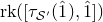 ${\mathrm{rk}}([\tau _{{\mathcal{S}}'}(\hat {1}), \hat {1}])$
.
Example 2.34. Consider the built lattice
 $({\mathcal{L}}_{\Gamma }, {\mathcal{G}}_{\Gamma })$
introduced in Example 2.25. The natural order on integers gives a total order
 $\vartriangleleft$
on the atoms of
 ${\mathcal{L}}_{\Gamma }$
. Let us describe the operadic normal monomials in
 $\mathbb{FY}^{\vee }({\mathcal{L}}_{\Gamma }, {\mathcal{G}}_{\Gamma })$
with respect to
 $\vartriangleleft$
, according to their weight (i.e. the cardinality of the corresponding nested set). The weight
 $2$
normal monomials are (in terms of nested sets)
 ${\mathcal{S}}(\omega ^{1}_{{\hat {0}}, \hat {1}}) = \{1, \hat {1}\}$
and
 $\{G, \hat {1}\}$
for all elements
 $G \in {\mathcal{G}}_{\Gamma }$
having rank
 $2$
or
 $3$
. The weight
 $3$
normal monomials are
 ${\mathcal{S}}(\omega ^{2}_{{\hat {0}}, \hat {1}}) = \{1, 123, \hat {1}\}$
, together with the nested sets
 $\{G, \hat {1}\}\circ (\omega ^0_{{\hat {0}}, G}, \omega ^1_{G, \hat {1}})$
for all
 $G\in {\mathcal{G}}_{\Gamma }$
of rank
 $2$
and
 $\{G, \hat {1}\} \circ (\omega ^1_{{\hat {0}}, G}, \omega ^0_{G, \hat {1}})$
for all
 $G\in {\mathcal{G}}_{\Gamma }$
of rank
 $3$
. In our example, the family ranging over rank
 $2$
elements gives the nested sets
 \begin{align*} &\{123, 12345, \hat {1}\}, \{145, 12345, \hat {1}\}, \{167, 12367, \hat {1}\}, \{24, 12345, \hat {1}\}, \{26, 12367, \hat {1}\}, \\&\quad\quad\quad\{46, 14567, \hat {1}\}, \{35, 12345, \hat {1}\}, \{37, 12367, \hat {1}\}, \textrm { and } \{57, 14567, \hat {1}\}, \end{align*}
and the family ranging over rank
 $3$
elements gives the nested sets
 \begin{align*} \{1, 12345, \hat {1}\}, \{1, 12367, \hat {1}\}, \{1, 14567, \hat {1}\}, \{2, 246, \hat {1}\}, \{3, 357, \hat {1}\}. \end{align*}
There is only one normal monomial of weight
 $4$
, which is given by the nested set
 \begin{align*} \{1, 123, 12345, \hat {1}\}. \end{align*}
3. The main results
This section is devoted to the proof of Theorem2.31. In § 3.1 we define an order on the simplicial generators of the Feichtner–Yuzvinsky algebras of supersolvable lattices and we compute the normal monomials of weight
 $2$
associated to this order. In § 3.2 we define a bijection between the algebraic normal monomials associated to the latter order and the operadic normal monomials described in § 2.5. The construction of this bijection will be done by induction and using the operadic structure. By a dimension argument this bijection will show that the algebraic normal monomials form an additive basis of the Feichtner–Yuzvinksky algebras, which will show that the set of quadratic relations forms a Gröbner basis of the Feichtner–Yuzvinsky algebras.
3.1 The order on generators and the normal monomials of weight 2
This subsection is devoted to defining an order on the simplicial generators of Feichtner–Yuzvinsky algebras and computing the associated quadratic normal monomials.
Definition 3.1. Let
 $({\mathcal{L}}, {\mathcal{G}})$
be a supersolvable built lattice, and
 $\vartriangleleft$
a total order on the atoms of
 $\mathcal{L}$
satisfying the property that for all pairs of atoms
 $H, H'$
, if there exists a
 $k$
such that
 $H \leq {\mathrm{d}}^k(\hat {1})$
and
 $H' \nleq {\mathrm{d}}^k(\hat {1})$
, then we have
 $H \vartriangleleft H'$
. For all
 $G \in {\mathcal{G}}$
, let
 $\mathsf{w}(G)$
denote the word with letters
 $\mathrm{At}_{\leq }(G)$
written in increasing order with respect to
 $\vartriangleleft$
. We define a total order on
 $\mathcal{G}$
, also denoted
 $\vartriangleleft$
, by setting
 \begin{align*} G \vartriangleleft G' \Leftrightarrow \mathsf{w}(G) \textrm { is strictly less than }\mathsf{w}(G') \textrm { for the lexicographic order.} \end{align*}
Remark 3.2. For all
 $G \in {\mathcal{G}}$
and all
 $k \leq {\mathrm{rk}} \, G - 1$
, we have the inequality
 \begin{equation} {\mathrm{d}}^{k}(G) \trianglelefteq G. \end{equation}
Furthermore, for all
 $G, G' \in {\mathcal{G}}$
with
 $G' \leq G$
and
 $G'$
not an initial segment of
 $G$
we have the inequality
 \begin{equation} G \vartriangleleft G'. \end{equation}
In what follows, whenever we introduce a supersolvable built lattice we implicitly choose a total order on
 $\mathcal{G}$
as in Definition 3.1. We shall see in Proposition 3.3 that the quadratic normal monomials with respect to
 $\vartriangleleft$
only depend on the subrelations (7), (8), which are determined solely by the supersolvable structure. This means that the additional choices made to define the total order
 $\vartriangleleft$
do not matter.
Proposition 3.3.
Let
 $({\mathcal{L}}, {\mathcal{G}})$
be a supersolvable built lattice, and let
 $\alpha = h_{G_1}h_{G_2}$
be a monomial in
 $\mathrm{FY}({\mathcal{L}}, {\mathcal{G}})$
with
 $G_1 \trianglelefteq G_2$
. Let us denote by
 $G$
the join
 $G_1 \vee G_2$
. For any admissible order on monomials induced by
 $\vartriangleleft$
, the monomial
 $\alpha$
is normal with respect to the quadratic relations of
 $\mathrm{FY}({\mathcal{L}},{\mathcal{G}})$
if and only if one of the following three conditions is verified.
-
– The element
$G$
does not belong to
$\mathcal{G}$
. -
– The element
$G$
belongs to
$\mathcal{G}$
, and
$G_1$
is an initial segment of
$G_2$
which is different from
$G_2$
. -
– The element
$G$
belongs to
$\mathcal{G}$
,
$G_2 \ngeq G_1$
,
$G_2$
is not covered by
$G$
and we have
$G_1 = {\mathrm{d}}^{k}(G)$
where
$k$
is the maximal integer satisfying
\begin{align*} {\mathrm{d}}^{k}(G) \vee G_2 = G. \end{align*}


For the rest of the article, for any two comparable elements
 $G \geq G'$
in
 $\mathcal{G}$
we will denote by
 $i_{G, G'}$
the biggest integer such that we have
 \begin{align*} {\mathrm{d}}^{i_{G, G'}}(G)\vee G' = G. \end{align*}
Proof.
We have an obvious bijection between the monomials described in the above proposition and the normal monomials given by Theorem2.30, sending
 $h_{{\mathrm{d}}^{{i_{G, G'}}}(G)}h_{G'}$
to
 $x_{G'}x_{G}$
if
 $G'$
is not covered by
 $G$
, sending
 $h_{{\mathrm{d}}(G)}h_G$
to
 $x_G^2$
and sending
 $h_{G_1}h_{G_2}$
to
 $x_{G_1}x_{G_2}$
when
 $\{G_1, G_2\}$
is a nested set of incomparable elements. By a dimension argument it is enough to prove that the quadratic normal monomials with respect to
 $\vartriangleleft$
are included in the monomials described in the proposition.
Assume
 $G = G_1 \vee G_2$
belongs to
 $\mathcal{G}$
. If
 $G \vartriangleleft G_1$
and
 $G \vartriangleleft G_2$
, then
 $h_{G_1}h_{G_2}$
is the leading term of the relation
 \begin{align*} (h_{G}-h_{G_1})(h_{G}- h_{G_2}). \end{align*}
If
 $G_1 \trianglelefteq G \vartriangleleft G_2$
and
 $G_2$
is covered by
 $G$
, then
 $h_{G_1}h_{G_2}$
is the leading term of the relation
 \begin{align*} (h_{G} - h_{G_1})(h_{G} - h_{G_2}) - h_{G}(h_{G} - h_{G_2}). \end{align*}
Finally, if
 $G_1 \trianglelefteq G \vartriangleleft G_2$
, then
 $G_1$
is some initial segment
 ${\mathrm{d}}^{k}(G)$
. If
 $k$
is not the maximal integer such that we have
 \begin{align*} {\mathrm{d}}^k(G)\vee G_2 = G, \end{align*}
we see that
 $h_{G_1}h_{G_2}$
is the leading term of the relation
 \begin{align*} (h_{G}-h_{G_1})(h_{G}-h_{G_2}) - (h_{G}-h_{{\mathrm{d}}^{k + 1}(G)})(h_{G} - h_{G_2}). \end{align*}
Example 3.4. Consider once again the built lattice
 $({\mathcal{L}}_{\Gamma }, {\mathcal{G}}_\Gamma )$
introduced in Example 2.25. The natural order on integers gives a total order on the atoms of
 ${\mathcal{L}}_\Gamma$
as in Definition 3.1, which leads to the total order
 $\vartriangleleft$
on
 ${\mathcal{G}}_\Gamma$
given by lexicographic order on the associated sets of atoms. Let us describe the quadratic normal monomials
 $h_{G_1}h_{G_2}$
of
 $\mathrm{FY}({\mathcal{L}}_\Gamma , {\mathcal{G}}_\Gamma )$
with respect to
 $\vartriangleleft$
, according to the join
 $G = G_1 \vee G_2$
. If
 $G$
has rank less than or equal to two then there is no normal monomial. If
 $G$
has rank three then there is exactly one normal monomial given by
 $h_{{\mathrm{d}}(G)}h_{G}$
. In our example, this gives the normal monomials
 \begin{align*} h_{123}h_{12345}, \,h_{123}h_{12367}, \,h_{145}h_{14567}, \,h_{24}h_{246}, \textrm { and } h_{35}h_{357}. \end{align*}
Finally if
 $G$
is equal to
 $\hat {1}$
then we have the monomial
 $h_{{\mathrm{d}}(\hat {1})}h_{\hat {1}} = h_{12345}h_{\hat {1}}$
and for each element
 $G'$
of rank
 $2$
we have the normal monomial
 $h_{{\mathrm{d}}^{i_{\hat {1},G'}}(\hat {1})}h_{G'}$
. In our example this gives the normal monomials
 \begin{align*} h_{\hat {1}}h_{123}, \, h_{\hat {1}}h_{145}, \,h_{12345}h_{167}, \,h_{\hat {1}}h_{24}, \,h_{12345}h_{26}, \,h_{123}h_{46}, \,h_{\hat {1}}h_{35}, \,h_{12345}h_{37}, \textrm { and } h_{123}h_{57}. \end{align*}
In weight
 $3$
there is only one normal monomial, which is given by
 $h_{123}h_{12345}h_{\hat {1}}$
.
We next come to an important lemma which highlights a first connection between our normal monomials and supersolvability.
Lemma 3.5.
Let
 $({\mathcal{L}}, {\mathcal{G}})$
be a supersolvable built lattice. Let
 $G_1$
and
 $G_2$
be two non-comparable elements of
 $\mathcal{G}$
such that we have
 $G_1 \vartriangleleft G_2$
,
 $G_1 \vee G_2 \in {\mathcal{G}}$
,
 $G_2$
is not covered by
 $G_1\vee G_2$
and
 $G_1$
is an initial segment of
 $G_1 \vee G_2$
. Then
 $h_{G_1}h_{G_2}$
is a normal monomial if and only if
 $G_1 \wedge G_2 \leq {\mathrm{d}}(G_1)$
.
The statement is not true without the supersolvability hypothesis. For instance, consider
 $\mathcal{L}$
the graphical lattice associated to a
 $5$
-cycle and number the edges (i.e. the atoms) from
 $1$
to
 $5$
. If we pick
 $G_1 = \{1, 2, 3 \}$
and
 $G_2 = \{4, 5\}$
in the maximal building set, then we have
 $G_1 \wedge G_2 = {\hat {0}}$
, but
 $h_{G_1}h_{G_2}$
is not normal because we have
 ${\mathrm{d}}(G_1) \vee G_2 = G_1 \vee G_2 = \hat {1}$
.
Proof.
With the hypothesis on
 $G_1$
and
 $G_2$
we have
 \begin{align*} h_{G_1}h_{G_2} \textrm { is normal } &\Leftrightarrow {\mathrm{d}}(G_1)\vee G_2 \lt G_1\vee G_2 \\ & \Leftrightarrow G_1 \nleq {\mathrm{d}}(G_1) \vee G_2 \\ & \Leftrightarrow G_1 \wedge ({\mathrm{d}}(G_1) \vee G_2) \lt G_1 \\ &\Leftrightarrow {\mathrm{d}}(G_1) \vee (G_1 \wedge G_2) \lt G_1 \\ &\Leftrightarrow G_1 \wedge G_2 \leq {\mathrm{d}}(G_1). \end{align*}
The fourth equivalence comes from the fact that, by supersolvability,
 $G_1$
is modular in the interval
 $[{\hat {0}}, G_1 \vee G_2]$
.
3.2 A bijection between algebraic normal monomials and operadic normal monomials
Let
 $({\mathcal{L}}, {\mathcal{G}})$
be a supersolvable built lattice and let
 $\vartriangleleft$
be a total order on the atoms of
 $\mathcal{L}$
obtained as in the proof of Definition 3.1. Let us denote by
 $\mathsf{ANM}({\mathcal{L}}, {\mathcal{G}}, \vartriangleleft )$
the set of algebraic normal monomials with respect to the order
 $\vartriangleleft$
and the quadratic relations. Let us denote by
 $\mathsf{ONM}({\mathcal{L}}, {\mathcal{G}}, \vartriangleleft )$
the set of operadic normal monomials with respect to the order on atoms
 $\vartriangleleft$
(see § 2.5). Notice that in the supersolvable case, the nested set
 ${\mathcal{S}}(\omega ^{k_G}_{\tau _{{\mathcal{S}}}(G), G})$
is simply some truncation of the maximal chain
 $\{G \gt {\mathrm{d}}_{\tau _{{\mathcal{S}}}(G)}(G) \gt {\mathrm{d}}^2_{\tau _{{\mathcal{S}}}(G)}(G) \gt \cdots \gt \tau _{{\mathcal{S}}}(G)\}$
. This means that the operadic normal monomials do not depend on the particular choice of
 $\vartriangleleft$
but only on the choice of the maximal chain of modular elements of
 $({\mathcal{L}}, {\mathcal{G}})$
. Such choice being implicit we will drop
 $\vartriangleleft$
from all notations.
3.2.1 From operadic normal monomials to algebraic normal monomials
We first define maps
 \begin{align*} \mathsf{ONM} ({\mathcal{L}}, {\mathcal{G}}) \xrightarrow {\Phi _{{\mathcal{L}}, {\mathcal{G}}}} \mathsf{ANM}({\mathcal{L}}, {\mathcal{G}}) \end{align*}
by induction on the rank of
 $\mathcal{L}$
. Let
 $({\mathcal{L}}, {\mathcal{G}})$
be a supersolvable built lattice. For any element
 $G \neq \hat {1} \in {\mathcal{G}}$
and any algebraic monomial
 $\alpha = \prod _{G'\in S} h_{G'}$
in
 $\mathrm{FY}([G, \hat {1}], \mathrm{Ind}({\mathcal{G}}))$
we define the algebraic monomial in
 $\mathrm{FY}({\mathcal{L}}, {\mathcal{G}})$
,
 \begin{align*} \mathsf{Supp}_G(\alpha ) = \prod _{\substack {G' \in S \\ G' \in {\mathcal{G}}}}h_{{\mathrm{d}}^{i_{G', G}}(G')} \prod _{\substack {G' \in S \\ G' \notin {\mathcal{G}}}} h_{G^{'\bot }}, \end{align*}
where for any
 $G' \notin {\mathcal{G}}$
, the element
 $G'^{\bot }$
is the factor of
 $G'$
in
 $\mathcal{G}$
different from
 $G$
. Finally, for any operadic normal monomial
 $\mathcal{S}$
in some supersolvable built lattice
 $({\mathcal{L}}, {\mathcal{G}}, \vartriangleleft )$
with
 $G$
the maximal element of
 ${\mathcal{S}}\setminus \{\hat {1}\}$
for the order
 $\vartriangleleft$
we define by induction (on both the cardinality of
 $\mathcal{S}$
and the rank of
 $\mathcal{L}$
) the map
 \begin{align*} \Phi _{{\mathcal{L}}, {\mathcal{G}}}({\mathcal{S}}) := \mathsf{Supp}_{G}(\Phi _{[G, \hat {1}], \mathrm{Ind}({\mathcal{G}})}(G\vee {\mathcal{S}}_{\nleq G})) \Phi _{[{\hat {0}}, G], \mathrm{Ind}({\mathcal{G}})}({\mathcal{S}}_{\leq G}) \end{align*}
initialized on singletons
 $\{\hat {1}\}$
by
 \begin{align*} \Phi _{{\mathcal{L}}, {\mathcal{G}}}(\{\hat {1}\}) = h_{\hat {1}} h_{{\mathrm{d}}(\hat {1})} \cdots h_{{\mathrm{d}}^{{\mathrm{rk}} {\mathcal{L}} - 2}(\hat {1})}. \end{align*}
One can check that
 $G\vee {\mathcal{S}}_{\nleq G}$
is an operadic monomial so our map is well defined. This map sends an operadic normal monomial to some algebraic monomial, which will turn out to be normal as a consequence of the proof of Theorem3.7.
3.2.2 From algebraic normal monomials to operadic normal monomials
We are concerned with finding an inverse for
 $\Phi$
. Let us define a candidate
 \begin{align*} \mathsf{ANM}({\mathcal{L}}, {\mathcal{G}}) \xrightarrow {\Psi _{{\mathcal{L}}, {\mathcal{G}}}} \mathsf{ONM}({\mathcal{L}}, {\mathcal{G}}) \end{align*}
by induction on the rank of
 $\mathcal{L}$
and the weight of the monomial. We will drop the built lattice from the notation if it can be deduced from the context. We initialize with
 \begin{align*} \Psi (1) = \omega _{{\hat {0}}, \hat {1}} = \{ \hat {1} \gt {\mathrm{d}}(\hat {1}) \gt \cdots \gt {\mathrm{d}}^{{\mathrm{rk}} \,{\mathcal{L}}-1}(\hat {1})\}. \end{align*}
Let
 $\alpha = \prod _{i} h_{G_i}$
be some algebraic normal monomial in
 $\mathrm{FY}({\mathcal{L}}, {\mathcal{G}})$
and let us denote by
 $G$
the maximum of the
 $G_i$
with respect to
 $\vartriangleleft$
. If
 $G = \hat {1}$
, then by Proposition 3.3 we see that all the
 $G_i$
except
 $G$
are below
 ${\mathrm{d}}(\hat {1})$
so we put
 \begin{align*} \Psi _{{\mathcal{L}}, {\mathcal{G}}}(\alpha ) = \Psi _{[{\hat {0}}, {\mathrm{d}}(\hat {1})], \mathrm{Ind}({\mathcal{G}})}(\alpha /h_{\hat {1}}), \end{align*}
where
 $ \Psi _{[{\hat {0}}, {\mathrm{d}}(\hat {1})], \mathrm{Ind}({\mathcal{G}})}(\alpha /h_{\hat {1}})$
is viewed as a normal monomial in
 $({\mathcal{L}}, {\mathcal{G}})$
(replacing
 ${\mathrm{d}}(\hat {1})$
by
 $\hat {1}$
). If
 $G$
is different from
 $\hat {1}$
, let us denote, respectively,
 \begin{align*} &\alpha _{\leq G} = \prod _{G_i \leq G} h_{G_i}, \\ &\alpha _{\nleq G} = \prod _{G_i \nleq G} h_{G_i}. \end{align*}
We put
 \begin{equation} \Psi _{{\mathcal{L}}, {\mathcal{G}}}(\alpha ) := \{G, \hat {1}\}\circ (\Psi _{[{\hat {0}}, G], \mathrm{Ind}({\mathcal{G}})}(\alpha _{\leq G}), \Psi _{[G, \hat {1}], \mathrm{Ind}({\mathcal{G}})}(G \vee \alpha _{\nleq G})), \end{equation}
with
 $G \vee \alpha _{\nleq G}$
a notation for
 $\prod _{G_i \nleq G}h_{G\vee G_i}$
. For this map to be well defined we must prove that the monomial
 $G\vee \alpha _{\nleq G}$
is normal in
 $\mathrm{FY}([G, \hat {1}], \mathrm{Ind}({\mathcal{G}}))$
. This is implied by the following lemma.
Lemma 3.6.
Let
 $({\mathcal{L}}, {\mathcal{G}})$
be a supersolvable built lattice and let
 $G_1 \vartriangleleft G_2 \vartriangleleft G_3$
be elements in
 $\mathcal{G}$
. If
 $h_{G_1}h_{G_2}$
,
 $h_{G_1}h_{G_3}$
and
 $h_{G_2}h_{G_3}$
are normal then
 $h_{G_1 \vee G_3}h_{G_2 \vee G_3}$
is normal in
 $\mathrm{FY}([G_3, \hat {1}], \mathrm{Ind}({\mathcal{G}}))$
.
This is the technical core of the article. The statement is not true in general without the supersolvability condition, as shown by the following example. Let
 $\mathcal{L}$
be the graphical lattice associated to a
 $6$
-cycle with edges
 $\{1, \ldots , 6\}$
. Consider the elements
 $G_1 = \{1, 2\}, G_2 = \{3,4\}$
and
 $G_3 = \{5,6\}$
. One can quickly check that the monomials
 $h_{G_1}h_{G_2}$
,
 $h_{G_1}h_{G_3}$
and
 $h_{G_2}h_{G_3}$
are normal in
 $\mathrm{FY}({\mathcal{L}}, {\mathcal{G}}_{\max })$
. However,
 $h_{G_1\vee G_3}h_{G_2 \vee G_3}$
is not normal in
 $\mathrm{FY}([G_3, \hat {1}], {\mathcal{G}}_{\max })$
for two reasons:
 $G_2 \vee G_3$
is covered by
 $G_1 \vee G_2 \vee G_3 = \hat {1}$
and we have
 \begin{align*} {1}\vee G_2 \vee G_3 = G_1 \vee G_2 \vee G_3. \end{align*}
If a built lattice has a small rank it can happen that it satisfies Lemma 3.6 without being supersolvable (see § 5.1).
Proof.
The statement is obvious when two of the
 $G_i$
are comparable so we can assume that the elements
 $G_1, G_2, G_3$
are not comparable. We make a disjunction on whether
 $G_i\vee G_j$
belongs to
 $\mathcal{G}$
for
 $i,j \leq 3$
.
Case 1.
 $G_i \vee G_j \notin {\mathcal{G}}$
for all
 $i \neq j \leq 3$
. In this case we have
 $(G_1\vee G_3)\vee (G_2 \vee G_3) \notin \mathrm{Ind}({\mathcal{G}})$
. Indeed, by the proof of Proposition 2.32 the element
 $G_1\vee G_2\vee G_3$
does not belong to
 $\mathcal{G}$
, and if
 $G_1\vee G_2\vee G_3$
is equal to
 $G_1 \vee G$
with
 $G \in {\mathcal{G}}$
and
 $G_1, G$
nested we immediately get
 $G_1 \vee G_2 = G \in {\mathcal{G}}$
, contradicting the initial hypothesis.
Case 2.
 $G_1 \vee G_2 \notin {\mathcal{G}}, G_1 \vee G_3 \notin {\mathcal{G}}, G_2 \vee G_3 \in {\mathcal{G}}$
. Let us show that
 $\{G_1 \vee G_3, G_2 \vee G_3\}$
is a nested set of pairwise incomparable elements in
 $\mathrm{Ind}({\mathcal{G}})$
as in Case 1. By contradiction, assume that
 $G_1 \vee G_2 \vee G_3$
belongs to
 $\mathcal{G}$
. By restriction, we can assume
 $G_1 \vee G_2 \vee G_3 = \hat {1}$
. Since
 $h_{G_2}h_{G_3}$
is normal and
 $G_2 \vee G_3 \in {\mathcal{G}}$
there exists some integer
 $k$
such that we have
 ${\mathrm{d}}^k(\hat {1})\wedge (G_2 \vee G_3) = G_2$
. We have
 \begin{align*} {\mathrm{d}}^{k}(\hat {1}) &= {\mathrm{d}}^k(\hat {1}) \wedge (G_2 \vee G_1 \vee G_3) \\ &= G_2 \vee ({\mathrm{d}}^k(\hat {1})\wedge (G_1 \vee G_3)) \\ &= G_2 \vee ({\mathrm{d}}^k(\hat {1})\wedge G_1) \wedge ({\mathrm{d}}^k(\hat {1}) \wedge G_3) \\ &\leq G_2 \vee G_1 \vee G_2 \\ &= G_1 \vee G_2. \end{align*}
By nested-ness this implies
 ${\mathrm{d}}^k(\hat {1}) =G_2$
which contradicts
 $G_1 \vartriangleleft G_2$
. If
 $G_1\vee G_2 \vee G_3$
belongs to
 $\mathrm{Ind}({\mathcal{G}})$
but not to
 $\mathcal{G}$
we immediately get a contradiction as in Case 1.
Case 3.
 $G_1 \vee G_2 \notin {\mathcal{G}}, G_1 \vee G_3 \in {\mathcal{G}}, G_2 \vee G_3 \notin {\mathcal{G}}$
. This is similar to Case 2.
Case 4.
 $G_1 \vee G_2 \notin {\mathcal{G}}, G_1 \vee G_3 \in {\mathcal{G}}, G_2 \vee G_3 \in {\mathcal{G}}$
. Once again, let us show that
 $\{G_1 \vee G_3, G_2 \vee G_3\}$
is a nested set of pairwise incomparable elements in
 $\mathrm{Ind}({\mathcal{G}})$
. By contradiction, assume that
 $G_1 \vee G_2 \vee G_3$
belongs to
 $\mathcal{G}$
. By restriction, we can assume that we have
 $G_1 \vee G_2 \vee G_3 = \hat {1}$
. By assumption, there exists an integer
 $k_1$
such that we have
 ${\mathrm{d}}^{k_1}(\hat {1}) \wedge (G_1\vee G_3) = G_1$
and an integer
 $k_2$
such that we have
 ${\mathrm{d}}^{k_2}(\hat {1}) \wedge (G_2 \vee G_3) = G_2$
. Let us denote
 $k := \min (k_1, k_2)$
. Let us assume
 $k_1 \geq k_2$
, the other case being symmetric. By modularity of
 ${\mathrm{d}}^k(\hat {1})$
and the definition of
 $k$
we have
 \begin{align*} {\mathrm{d}}^{k}(\hat {1}) &= {\mathrm{d}}^k(\hat {1}) \wedge (G_1 \vee G_2 \vee G_3) \\ &= G_1 \vee ({\mathrm{d}}^k(\hat {1})\wedge (G_2 \vee G_3)) \\ &= G_1 \vee G_2. \end{align*}
This contradicts the fact that
 $G_1 \vee G_2$
does not belong to
 $\mathcal{G}$
. If
 $G_1 \vee G_2 \vee G_3$
belongs to
 $\mathrm{Ind}({\mathcal{G}})$
and not to
 $\mathcal{G}$
we immediately get a contradiction as in the previous cases.
Case 5.
 $G_1 \vee G_2 \in {\mathcal{G}}$
,
 $G_1 \vee G_3 \notin {\mathcal{G}}$
and
 $G_2 \vee G_3 \notin {\mathcal{G}}$
. We can either have
 $G_1 \vee G_2 \vee G_3 \notin {\mathcal{G}}$
or the contrary. In the first case the building set isomorphism
 \begin{align*} [{\hat {0}} ,G_1 \vee G_2 \vee G_3 ] \simeq [{\hat {0}}, G_1\vee G_2 ]\times [{\hat {0}}, G_3] \end{align*}
immediately gives the result. In the second case we can assume
 $G_1 \vee G_2 \vee G_3 = \hat {1}$
. Let us prove that
 $G_1\vee G_3$
is an initial segment of
 $G_1\vee G_2\vee G_3$
in
 $[G_3, \hat {1}]$
. By assumption, there exists an integer
 $k$
such that we have
 ${\mathrm{d}}^{k}(\hat {1}) \wedge (G_1 \vee G_2) = G_1$
. We will prove the equality
 \begin{align*} {\mathrm{d}}^{k}(\hat {1}) \vee G_3 = G_1 \vee G_3. \end{align*}
We have
 \begin{align*} {\mathrm{d}}^{k}(\hat {1}) &= {\mathrm{d}}^{k}(\hat {1})\wedge (G_1 \vee G_2 \vee G_3) \\ &= G_1 \vee ({\mathrm{d}}^{k}(\hat {1}) \wedge (G_2 \vee G_3)) \, (\textrm {by modularity of } {\mathrm{d}}^{k}(\hat {1})) \\ &\leq G_1 \vee ({\mathrm{d}}^{k}(\hat {1}) \wedge G_2) \vee ({\mathrm{d}}^k(\hat {1}) \wedge G_3) \, ( \textrm {by nested-ness of } \{G_2, G_3\})\\ &\leq G_1 \vee G_1 \vee G_3 \, (\textrm {by definition of } k) \\ & = G_1\vee G_3. \end{align*}
The other inequality is obvious. Let us now show the inequality
 \begin{equation} {\mathrm{d}}(G_1)\vee G_2 \vee G_3 \lt G_1 \vee G_2 \vee G_3. \end{equation}
According to Lemma 3.5 it is enough to prove the inequality
 \begin{equation} (G_1\vee G_3) \wedge (G_2 \vee G_3) \leq {\mathrm{d}}(G_1) \vee G_3. \end{equation}
An atom
 $H$
below
 $G_1 \vee G_3$
is either below
 $G_1$
or
 $G_3$
by nested-ness, and similarly for
 $G_2 \vee G_3$
. As a consequence, an atom below
 $G_1 \vee G_3$
and below
 $G_2\vee G_3$
is either below
 $G_3$
or is below
 $G_1 \wedge G_2$
, which is below
 ${\mathrm{d}}(G_1)$
by Lemma 3.5.
One must also prove that
 $G_2 \vee G_3$
is not covered by
 $G_1\vee G_2 \vee G_3$
. By inequality (10), if
 $G_2\vee G_3$
is covered by
 $G_1 \vee G_2 \vee G_3$
then we have
 ${\mathrm{d}}(G_1)\vee G_3 \leq G_2 \vee G_3$
. In this case, by nested-ness
 ${\mathrm{d}}(G_1)$
is either below
 $G_2$
or
 $G_3$
. In the first case we immediately obtain that
 $G_2$
is covered by
 $G_1\vee G_2$
, which is a contradiction. In the second case we get
 $G_1 \wedge G_3 \neq {\hat {0}}$
, which contradicts the fact that
 $G_1\vee G_3$
does not belong to
 $\mathcal{G}$
.
Case 6.
 $G_1 \vee G_2 \in {\mathcal{G}}$
,
 $G_2 \vee G_3 \in {\mathcal{G}}$
. In this case we necessarily have
 $G_1 \vee G_2 \vee G_3 \in {\mathcal{G}}$
. Let us prove that
 $G_1 \vee G_3$
is an initial segment of
 $G_1 \vee G_2 \vee G_3$
in
 $[G_3, G_1 \vee G_2 \vee G_3]$
. It is enough to prove that
 $G_1$
is an initial segment of
 $G_1 \vee G_2 \vee G_3$
. By restriction, we can assume
 $G_1 \vee G_2 \vee G_3 = \hat {1}$
. Since
 $G_1$
is an initial segment of
 $G_1 \vee G_2$
there exists an integer
 $k_1$
such that we have
 ${\mathrm{d}}^{k_1}(\hat {1})\wedge (G_1 \vee G_2) = G_1$
. Since
 $G_2$
is an initial segment of
 $G_2 \vee G_3$
, there exists an integer
 $k_2$
such that we have
 ${\mathrm{d}}^{k_2}(\hat {1})\wedge (G_2 \vee G_3) = G_2$
. The integer
 $k_1$
is greater than or equal to
 $k_2$
because the opposite inequality would imply
 $G_2 \leq G_1$
. Let us prove the equality
 \begin{align*} {\mathrm{d}}^{k_1}(\hat {1}) = G_1. \end{align*}
We have
 \begin{align*} {\mathrm{d}}^{k_1}(\hat {1}) &= {\mathrm{d}}^{k_1}(\hat {1})\wedge (G_1 \vee G_2 \vee G_3) \\ &= G_1 \vee ({\mathrm{d}}^{k_1}(\hat {1}) \wedge (G_2 \vee G_3)) \, (\textrm {by modularity of } {\mathrm{d}}^{k_1}(\hat {1})) \\ &\leq G_1 \vee ({\mathrm{d}}^{k_1}(\hat {1}) \wedge G_2) \, ( \textrm {by } k_1 \geq k_2)\\ &\leq G_1 \vee G_1 \, (\textrm {by definition of } k_1) \\ & = G_1. \end{align*}
The opposite inequality is obvious. Let us now prove inequality (11). By modularity of
 $G_1= {\mathrm{d}}^{k_1}(\hat {1})$
we have
 \begin{align*} (G_1 \vee G_3)\wedge (G_2 \vee G_3) &= (G_1 \wedge (G_2 \vee G_3)) \vee (G_3 \wedge (G_2 \vee G_3)) \\ &= (G_1 \wedge (G_2 \vee G_3) ) \vee G_3 \\ &\leq (G_1 \wedge G_2) \vee G_3 \, (\textrm {by } k_1 \geq k_2) \\ &\leq {\mathrm{d}}(G_1) \vee G_3. \end{align*}
As in the other cases, one can check that
 $G_2 \vee G_3$
is not covered by
 $G_1 \vee G_2 \vee G_3$
.
Case 7.
 $G_1 \vee G_2 \in {\mathcal{G}}$
,
 $G_1 \vee G_3 \in {\mathcal{G}}$
,
 $G_2 \vee G_3 \notin {\mathcal{G}}$
. In this case, we necessarily have
 $G_1\vee G_2 \vee G_3 \in {\mathcal{G}}$
. As always, by restriction we can assume
 $G_1 \vee G_2 \vee G_3 = \hat {1}$
. By assumption, there exists an integer
 $k_2$
such that we have
 ${\mathrm{d}}^{k_2}(\hat {1}) \wedge (G_1 \vee G_2) = G_1$
and an integer
 $k_3$
such that we have
 ${\mathrm{d}}^{k_3}(\hat {1}) \wedge (G_1 \vee G_3) = G_1$
. Let us denote
 $k := \max (k_2, k_3)$
. We will prove the equality
 \begin{align*} {\mathrm{d}}^{k}(\hat {1}) = G_1. \end{align*}
We have
 \begin{align*} {\mathrm{d}}^{k}(\hat {1}) &= {\mathrm{d}}^{k}(\hat {1})\wedge (G_1 \vee G_ 2\vee G_3) \\ &= G_1 \vee ({\mathrm{d}}^k(\hat {1})\wedge (G_2 \vee G_3)) \, (\textrm {by modularity of } {\mathrm{d}}^k(\hat {1}))\\ &= G_1 \vee ({\mathrm{d}}^k(\hat {1})\wedge G_2) \vee ({\mathrm{d}}^{k}(\hat {1}) \wedge G_3) \, (\textrm {by nested-ness of } \{G_2, G_3\})\\ &\leq G_1 \vee G_1 \, (\textrm {by the definition of } k)\\ &= G_1. \end{align*}
The opposite inequality is obvious. This implies that
 $G_1 \vee G_3$
is an initial segment of
 $G_1 \vee G_2 \vee G_3$
in
 $[G_3, \hat {1}]$
. Let us now prove inequality (11). By modularity of
 $G_1= {\mathrm{d}}^{k_1}(\hat {1})$
we have

As in the other cases, one can check that
 $G_2 \vee G_3$
is not covered by
 $G_1 \vee G_2 \vee G_3$
.
3.3 Proof of the main theorem
In this section we give the proof of our main theorem and some immediate corollaries.
Theorem 3.7.
Let
 $({\mathcal{L}}, {\mathcal{G}})$
be a supersolvable built lattice. The algebra
 $\mathrm{FY}({\mathcal{L}}, {\mathcal{G}})$
admits a quadratic Gröbner basis.
Proof.
By dimension, it is enough to prove that the map
 $\Phi$
is a left inverse of
 $\Psi$
, which we will do by induction. The base cases are obvious. Let
 $\alpha = \prod _{G' \in S} h_{G'}$
be a normal algebraic monomial with maximal element
 $G$
with respect to
 $\vartriangleleft$
. If
 $G = \hat {1}$
, then every element
 $G' \in S$
is of the form
 ${\mathrm{d}}^{k}(\hat {1})$
for some
 $k$
. In this case we can explicitly compute
 \begin{align*} \Psi \biggl(\prod _{i \leq n} h_{{\mathrm{d}}^{k_i}(\hat {1})}\biggr) = \{{\mathrm{d}}^{k}(\hat {1}) \, | \, k+1 \notin \{k_i, i \leq n \}\}, \end{align*}
and
 \begin{align*} \Phi (\{{\mathrm{d}}^{k_i}(\hat {1}), \, i \leq n \}) = \prod _{ k-1 \notin \{k_i, i \leq n \}} h_{{\mathrm{d}}^{k}(\hat {1})}, \end{align*}
which proves reciprocity. If
 $G \neq \hat {1}$
, by induction one can prove that the maximal element (for
 $\vartriangleleft$
) of
 $\Psi (\alpha )$
is
 $G$
. We then have, by definition,
 \begin{align*} \Phi \circ \Psi (\alpha ) &= \Phi (\{G, \hat {1}\}\circ (\Psi (G \vee \alpha _{\nleq G}), \Psi (\alpha _{\leq G}))) \\ &= \mathsf{Supp}_{G}(\Phi (\Psi (G\vee \alpha )))\Phi (\Psi (\alpha _{\leq G})). \end{align*}
However, by normality of
 $\alpha$
and maximality of
 $G$
we get
 $\mathsf{Supp}_{G}(G \vee \alpha ) = \alpha _{\nleq G}$
, which concludes the proof by induction.
We have an immediate corollary.
Corollary 3.8.
Let
 $({\mathcal{L}}, {\mathcal{G}})$
be a supersolvable built lattice. The algebra
 $\mathrm{FY}({\mathcal{L}}, {\mathcal{G}})$
is Koszul.
For completeness, let us record here a presentation of the Koszul dual Lie algebra of
 $\mathrm{FY}({\mathcal{L}}, {\mathcal{G}})$
for any built lattice
 $({\mathcal{L}}, {\mathcal{G}})$
such that
 $\mathrm{FY}({\mathcal{L}}, {\mathcal{G}})$
is quadratic. To the best of our knowledge, such a presentation has not yet appeared in the literature. It is a direct generalization of the presentation given in [Reference DotsenkoDot22, Theorem 4.3] in the case of complete graphs with minimal building sets.
Proposition 3.9.
Let
 $({\mathcal{L}}, {\mathcal{G}})$
be a built lattice. The Koszul dual Lie algebra of
 $\mathrm{FY}({\mathcal{L}}, {\mathcal{G}})$
is isomorphic to the graded Lie algebra generated by elements
 $y_G$
of degree
 $1$
, where
 $G\in {\mathcal{L}}$
has rank greater than or equal to
 $2$
, subject to the relations
 \begin{align*} [y_{G_1}, y_{G_2}] = 0\quad \textrm {for all nested sets } \{G_1, G_2\} \textrm { of incomparable elements}, \end{align*}
 \begin{align*} \sum _{\substack {G_1, G_2 \textrm { s.t.}\\ G_1 \vee G_2 = G}}[y_{G_1}, y_{G_2}] = 0 \quad\textrm {for all } G \textrm { of rank greater than or equal to 3, } \end{align*}
 \begin{align*} \biggl[y_{G_1}, \sum _{G_1 \vee G_2 = G}y_{G_2}\biggr] = 0\quad \textrm {for all } G, G_1 \textrm { such that we have } G \geq G_1 \textrm { and } {\mathrm{rk}} \, G \gt {\mathrm{rk}} \, G_1 + 1. \end{align*}
Proof.
We must prove that the above relations span the annihilator of the quadratic relations of
 $\mathrm{FY}({\mathcal{L}}, {\mathcal{G}})$
. By direct inspection one can check that the above relations belong to the annihilator. Furthermore, those relations are linearly independent because monomials appearing in the first set of relations do not appear in the relations of the second set and third set, relations of the second set each contain one monomial of the form
 $[y_G, y_G]$
(different for each relation), which do not appear in the relations of the third set, and relations of the third set each contain one monomial of the form
 $[y_{G_1}, y_G], G_1 \leq G$
which is different for each relation. Finally, one can check that those relations have the right cardinality, which concludes the proof.
When restricting our attention to the maximal building set we get the following corollary of Theorem2.31.
Corollary 3.10.
Let
 $\mathcal{L}$
be a supersolvable lattice. The combinatorial Chow ring
 $\mathrm{FY}({\mathcal{L}}, {\mathcal{G}}_{\max })$
admits a quadratic Gröbner basis.
In § 3.4 we shall see that this is also true for the minimal building set.
3.4 Minimal building sets of supersolvable lattices
A lattice is said to be irreducible if it is not a product of proper subposets. The minimal building set
 ${\mathcal{G}}_{\min }$
of a lattice
 $\mathcal{L}$
is the set of elements
 $F$
of
 $\mathcal{L}$
such that
 $[{\hat {0}}, F]$
is irreducible. We have the following proposition.
Proposition 3.11.
Let
 $\mathcal{L}$
be an irreducible supersolvable lattice. The built lattice
 $({\mathcal{L}}, {\mathcal{G}}_{\min })$
is supersolvable.
Proof.
It is enough to prove that if
 $\mathcal{L}$
is a supersolvable irreducible lattice then
 ${\mathrm{d}}(\hat {1})$
is irreducible. In fact, here
 ${\mathrm{d}}(\hat {1})$
can be any modular coatom (it does not need to be part of a maximal chain of modular elements). We will prove the contraposition of this statement. Assume that
 $[{\hat {0}}, {\mathrm{d}}(\hat {1})]$
decomposes as a product
 $[{\hat {0}}, F_1]\times \cdots \times [{\hat {0}}, F_n]$
. Denote by
 $R$
the set of atoms that are not below
 ${\mathrm{d}}(\hat {1})$
. We have the following lemma.
Lemma 3.12.
There exists an integer
 $i\leq n$
such that we have the inclusion
 $(\bigvee R) \setminus R \subset F_i$
.
Proof. Recall from § 2.1 that we have
 \begin{align*} \bigvee R = \sigma (R) = R \cup \{i \in \mathrm{At}({\mathcal{L}}) \, | \, \exists \, C \textrm { circuit s.t. } i \in C \subset R \cup \{i\}\}. \end{align*}
Let us prove that there exists some integer
 $i$
such that for any atom
 $H \notin R$
and any circuit
 $C \subset R \cup \{H\}$
containing
 $H$
we have
 $H \leq F_i$
, by induction on the cardinality of the circuits. The base case is when the circuits have length
 $3$
. Let
 $H_1$
,
 $H_2$
be two different atoms in
 $R$
. Since
 ${\mathrm{d}}(\hat {1})$
is a coatom we have
 $H_2 \leq \hat {1} = {\mathrm{d}}(\hat {1}) \vee H_1$
so there exists a circuit
 $C$
containing
 $H_1$
and
 $H_2$
and such that we have
 $C\setminus \{H_1, H_2\} \subset {\mathrm{d}}(\hat {1})$
. Since
 ${\mathrm{d}}(\hat {1})$
is modular by Lemma 2.26, there exists a circuit
 $C'$
containing some element
 $H'$
in
 ${\mathrm{d}}(\hat {1})$
and such that
 $C'\setminus \{H'\}$
is equal to
 $\{H_1, H_2\}$
. Such a circuit is in fact unique, the atom
 $H'$
being necessarily equal to
 ${\mathrm{d}}(\hat {1})\wedge (H_1 \vee H_2)$
. Now consider three atoms
 $H_1, H_2, H_3$
in
 $R$
. The element
 ${\mathrm{d}}(\hat {1}) \wedge (H_1 \vee H_2 \vee H_3)$
has rank at most
 $2$
and contains the three atoms
 ${\mathrm{d}}(\hat {1})\wedge (H_i \vee H_j)$
for
 $i \neq j \leq 3$
. If two of those atoms are equal, say
 \begin{align*} {\mathrm{d}}(\hat {1}) \wedge (H_1 \vee H_2) = {\mathrm{d}}(\hat {1}) \wedge (H_2 \vee H_3) =: H, \end{align*}
then by sub-modularity of
 $\mathcal{L}$
we have
 \begin{align*} \rho (H_1 \vee H_3 \vee H) \leq \rho (H_1 \vee H) + \rho (H_3\vee H) - \rho ((H_1\vee H) \wedge (H_3\vee H)) \leq 2 + 2 -2 = 2 \end{align*}
(since we have
 $H \vee H_2 \leq (H_1 \vee H) \wedge (H_3 \vee H)$
). This implies that
 $H \leq H_1 \vee H_3$
, and therefore
 ${\mathrm{d}}(\hat {1}) \wedge (H_1 \vee H_3)$
is also equal to
 $H$
. If the three atoms are different then they must form a circuit, and thus they must all belong to some same
 $F_i$
. This concludes the initialization. Let us now assume that all the atoms
 ${\mathrm{d}}(\hat {1})\wedge (H_1 \vee H_2)$
are, for instance, below
 $F_1$
.
Let
 $C$
be a circuit of arbitrary length containing a unique element
 $H$
not in
 $R$
. Let
 $H_1, H_2$
be two atoms in
 $C$
different from
 $H$
. By the initialization part there exists a circuit
 $\{H_1, H_2, H'\}$
with
 $H'$
in
 $F_1$
. If
 $H'$
is equal to
 $H$
then we have
 $H \in F_1$
. If not, by Axiom (1), one can construct a circuit
 $C'$
containing
 $H$
and not containing
 $H_1$
, such that
 $C'$
is included in
 $C\cup \{H'\}$
. If
 $C'$
does not contain
 $H'$
, then we are done by induction. If
 $C'$
contains
 $H'$
then since
 ${\mathrm{d}}(\hat {1})$
is modular by Lemma 2.26, there exists a circuit
 $C''$
containing some element
 $H''$
in
 ${\mathrm{d}}(\hat {1})$
and such that
 $C''\setminus \{H''\}$
is contained in
 $C'\cap R$
. By induction, the atom
 $H''$
belongs to
 $F_1$
. If
 $H'' = H$
we are done. Otherwise, by Axiom (1) there exists a circuit
 $C'''$
containing
 $H$
, contained in
 $C' \cup \{H'' \}$
and not containing some element in
 $C' \cap R$
. Reiterating this process we get a circuit containing
 $H$
and some elements in
 $F_1$
which proves that
 $H$
belongs to
 $F_1$
.
From this we deduce the second lemma.
Lemma 3.13.
The set of atoms
 $F_1 \cup R$
is closed.
Proof.
Let
 $H$
be some element contained in a circuit
 $C$
contained in
 $F_1 \cup R \cup \{H\}$
. If
 $H$
is in
 $R$
we are done. If
 $H$
is the unique element of
 $C$
under
 ${\mathrm{d}}(\hat {1})$
, then by the Lemma 3.12 we are also done. Otherwise, using Lemma 2.26 together with Axiom (1) (as we did in Lemma 3.12) gives us a circuit contained in
 ${\mathrm{d}}(\hat {1})$
, containing
 $H$
with every other element in
 $F_1$
. This proves that
 $H$
belongs to
 $F_1$
.
Finally, we get the concluding lemma.
Lemma 3.14. The lattice
 $\mathcal{L}$
is isomorphic to
 $[{\hat {0}}, F_1\cup R]\times [{\hat {0}}, F_2] \times \cdots \times [{\hat {0}}, F_n]$
.
Proof.
We will prove that every circuit is either contained in
 $F_1 \cup R$
or in some
 $F_i$
with
 $i \geq 2$
. Let
 $C$
be a circuit in
 $\mathcal{L}$
. If
 $C$
is contained in
 ${\mathrm{d}}(\hat {1})$
then the result comes from the isomorphism
 $[{\hat {0}}, {\mathrm{d}}(\hat {1})] \simeq [{\hat {0}}, F_1] \times \cdots \times [{\hat {0}}, F_n]$
. If
 $C \nsubseteq {\mathrm{d}}(\hat {1})$
and if
 $C\cap {\mathrm{d}}(\hat {1})$
is a singleton, then by the previous lemma we have
 $C \subset F_1 \cup R$
. If
 $C\nsubseteq {\mathrm{d}}(\hat {1})$
and if
 $C \cap {\mathrm{d}}(\hat {1})$
is not a singleton, pick
 $H$
any atom in
 $C\cap {\mathrm{d}}(\hat {1})$
. By iterating Lemma 2.26 as in the proof of Lemma 3.13 we obtain a circuit
 $C'$
containing
 $H$
, contained in
 ${\mathrm{d}}(\hat {1})$
and containing some elements in
 $F_1$
. The isomorphism
 \begin{align*} [{\hat {0}}, {\mathrm{d}}(\hat {1})] \simeq [{\hat {0}}, F_1]\times \cdots \times [{\hat {0}}, F_n] \end{align*}
implies that this circuit should be contained in
 $F_1$
, which proves the result.
Proposition 3.11 and Theorem2.31 imply the following theorem.
Theorem 3.15.
Let
 $\mathcal{L}$
be a supersolvable lattice. The algebra
 $\mathrm{FY}({\mathcal{L}}, {\mathcal{G}}_{\min })$
has a quadratic Gröbner basis and is therefore Koszul.
Proof.
Any supersolvable lattice
 $\mathcal{L}$
decomposes as a product of irreducible supersolvable lattices
 \begin{align*} {\mathcal{L}} \simeq {\mathcal{L}}_1 \times \cdots \times {\mathcal{L}}_n. \end{align*}
We then have
 \begin{align*} \mathrm{FY}({\mathcal{L}}, {\mathcal{G}}_{\min }) \simeq \mathrm{FY}({\mathcal{L}}_1, {\mathcal{G}}_{\min })\otimes \cdots \otimes \mathrm{FY}({\mathcal{L}}_n, {\mathcal{G}}_{\min }), \end{align*}
4. Application to the extended modular operad
4.1 Chordal graphs
In [Reference StanleySta72], Stanley proved that if
 $\Gamma$
is a chordal graph (meaning every cycle of length greater than or equal to
 $4$
in
 $\Gamma$
has a chord), the geometric lattice associated to
 $\Gamma$
is supersolvable. This result is based on the following lemma by Dirac [Reference DiracDir61].
Lemma 4.1 (Dirac [Reference DiracDir61]). Every chordal graph admits a vertex
 $v$
such that the graph induced by the neighbors of
 $v$
is a complete graph.
Such vertices are called ‘simplicial’. If we remove a simplicial vertex from a chordal graph, the graph we obtain is chordal and this graph is a coatom in the original graph. This means we can reiterate the process and get a maximal chain in the lattice associated with a chordal graph. One can then check that this maximal chain consists of modular elements. We have a ‘built’ variant of this result. Let us remind the reader that in Example 2.10 we defined a built lattice
 $({\mathcal{L}}_\Gamma , {\mathcal{G}}_\Gamma )$
for every simple graph
 $\Gamma$
, with
 ${\mathcal{L}}_\Gamma$
the usual graphical matroid associated to
 $\Gamma$
and
 ${\mathcal{G}}_\Gamma$
the building set of connected subgraphs of
 $\Gamma$
.
Lemma 4.2.
Let
 $\Gamma$
be a connected chordal graph. The built lattice
 $({\mathcal{L}}_\Gamma , {\mathcal{G}}_\Gamma )$
associated to
 $\Gamma$
is supersolvable.
Proof.
Let us choose a maximal chain of modular elements as in the last paragraph. By construction, those elements are connected subgraphs of
 $\Gamma$
. Let
 $G$
be a closed connected subset of edges of
 $\Gamma$
. For any integer
 $k$
less than the rank of
 ${\mathcal{L}}_{\Gamma }$
, the element
 ${\mathrm{d}}^{k}(\hat {1}) \wedge G$
can be obtained from
 $G$
by successively removing simplicial vertices of
 $G$
, and therefore it is connected.
Corollary 4.3.
For all chordal graphs
 $\Gamma$
, the Feichtner–Yuzvinsky algebra
 $\mathrm{FY}({\mathcal{L}}_\Gamma , {\mathcal{G}}_\Gamma )$
admits a quadratic Gröbner basis and is therefore Koszul.
4.2 The components of the extended modular operad
In [Reference Losev and ManinLM00], Losev and Manin introduced new moduli stacks
 $\overline {L}_{g,S}$
for stable curves of genus
 $g$
with painted marked points indexed by
 $S$
of two types (say ‘black’ and ‘white’), where the points of type black are allowed to coincide and the points of type white are not. Those stacks are the components of the so-called extended modular operad (see [Reference Losev and ManinLM04]). We will deduce from Corollary 4.3 the following result.
Theorem 4.4. The cohomology algebras of the components of the extended modular operads in genus 0 are Koszul.
Proof.
It is part of the folklore that if
 $S$
is a (colored) set with
 $m$
white points and
 $n$
black points and that
 $*$
is some chosen white point, then the moduli space
 $\overline {L}_{0, S}$
is isomorphic to the wonderful compactification of the graphical arrangement
 \begin{align*} {\mathcal{H}}_{m,n} = \{z_i = z_j \, | \,i \neq * \textrm { white }, \, j \neq * \textrm { white or black} \}, \end{align*}
with respect to the building set of connected components (see Example 2.10). Here, let us summarize the main line of arguments leading to this isomorphism. In [Reference ManinMan04], Manin remarked that the moduli stacks
 $\overline {L}_{g, S}$
are part of the formalism of Hassett spaces introduced by Hassett in [Reference HassettHas03]. In the latter article, the author introduces the moduli problem of curves with weighted points, where one fixes a ‘weight data’ consisting of a vector
 $(g, \mathsf{w}) = (g, w_1, \ldots , w_n) \in \mathbb{N} \times (]0 , 1] \cap \mathbb{Q})^n$
and then seeks to parametrize the nodal curves of genus
 $g$
with
 $n$
marked points
 $(s_i)_{i \leq n}$
which are allowed to coincide ‘up to their weights’, meaning that if the points
 $s_i, i \in I$
coincide, then we require
 \begin{align*} \sum _{i \in I}w_i \leq 1, \end{align*}
and a (weighted) stability condition is satisfied (see [Reference HassettHas03]). If the first
 $p$
weights are
 $1$
and the last
 $n-p$
weights are small enough (precisely,
 $\sum _{i \gt p} w_i \lt 1$
) then the above condition means exactly that the first
 $p$
points cannot coincide with any other point and the last
 $n-p$
points can coincide only between them, and we recover the painted moduli problem of Losev and Manin. Hassett proved that there exists a Deligne–Mumford stack
 $\overline {{\mathcal{M}}}_{g, \mathsf{w}}$
representing the above weighted moduli problem.
In genus
 $0$
, the stability condition can be simply stated: for any irreducible component
 $T$
of the nodal curve, we require
 \begin{align*} \sum _{i \,\textrm {s.t.}s_i \in T} w_i + \#\textrm {nodes of } T \gt 2. \end{align*}
In addition, in genus
 $0$
the moduli stack
 $\overline {{\mathcal{M}}}_{0, \mathsf{w}}$
is a smooth projective scheme (called a Hassett space). If the weights are either
 $1$
or very small then we call those Hassett spaces ‘heavy/light’. Indices with weight
 $1$
are called heavy and the other indices are called light. The work of Cavalieri, Hampe, Markwig and Ranganathan [Reference Cavalieri, Hampe, Markwig and RanganathanCHMR16] shows that a ‘heavy/light’ Hassett space is a ‘tropical compactification’ of the projective complement
 ${\mathcal{M}}_{0, \mathsf{w}}$
of the same graphical arrangement
 $\{z_i = z_j \, | \,i \neq * \textrm { heavy}, \, j \neq * \textrm { heavy or light} \}$
(with
 $*$
some chosen heavy index). Let us briefly explain what this means, referring to [Reference MacLagan and SturmfelsMS15] for more details. One possible starting point is to consider a tropical version
 ${\mathcal{M}}^{\mathrm{trop}}_{0, \mathsf{w}}$
of
 ${\mathcal{M}}_{0, \mathsf{w}}$
, which consists of the set of all metric trees with leaves labeled from one to
 $n$
, satisfying some stability condition depending on
 $\mathsf{w}$
(those are the so-called tropical
 $\mathsf{w}$
-stable curves (of genus zero)). The space
 ${\mathcal{M}}^{\mathrm{trop}}_{0, \mathsf{w}}$
has the structure of an abstract cone complex, which can be realized as a fan in a lattice. On the geometric end, the moduli space
 ${\mathcal{M}}_{0, \mathsf{w}}$
can be embedded in the torus associated to the same lattice using the Plücker coordinates. Via this embedding, the closure of
 ${\mathcal{M}}_{0, \mathsf{w}}$
in the toric variety associated to the fan
 ${\mathcal{M}}^{\mathrm{trop}}_{0, \mathsf{w}}$
is exactly the Hassett space
 $\overline {{\mathcal{M}}}_{0, \mathsf{w}}$
. The fan realizing
 ${\mathcal{M}}^{\mathrm{trop}}_{0, \mathsf{w}}$
is none other than the Bergman fan associated to the built lattice
 $({\mathcal{L}}_{\Gamma _{m,n}}, {\mathcal{G}}_{\Gamma _{m,n}})$
(see [Reference Feichtner and YuzvinskyFY04] for the definition of the Bergman fan of a built lattice), with
 $\Gamma _{m,n}$
the graph giving the arrangement
 ${\mathcal{H}}_{m,n}$
.
In [Reference TevelevTev07], Tevelev showed that the tropical compactification of a projective hyperplane arrangement complement along the Bergman fan of some building set
 $\mathcal{G}$
of the corresponding lattice can in fact be identified with the wonderful compactification of De Concini and Procesi along the same building set
 $\mathcal{G}$
, which is the stated isomorphism.
We notice that the graph
 $\Gamma _{m,n}$
is chordal for every
 $m$
and
 $n$
, which concludes the proof by Corollary 4.3.
5. Further considerations
5.1 Towards a classification of Koszul–Feichtner–Yuzvinsky algebras
We would like to emphasize the fact that we know plenty of Feichtner–Yuzvinsky algebras
 $\mathrm{FY}({\mathcal{L}}, {\mathcal{G}})$
that admit quadratic Gröbner bases and such that the built lattice
 $({\mathcal{L}}, {\mathcal{G}})$
is not supersolvable, especially in low rank. For instance, if
 $C_4$
and
 $C_5$
are, respectively, the
 $4$
- and
 $5$
-cycles, then the lattices
 ${\mathcal{L}}_{C_4}$
and
 ${\mathcal{L}}_{C_5}$
are not supersolvable but the built lattices
 $({\mathcal{L}}_{C_4}, {\mathcal{G}}_{C_4})$
and
 $({\mathcal{L}}_{C_5}, {\mathcal{G}}_{C_5})$
are so small that they still satisfy the key Lemma 3.6, and therefore their Feichtner–Yuzvinsky algebras will be Koszul. However, for the wonderful presentation and for the order used in this article, based on a few examples it feels to the author that the supersolvability condition should be close to necessary, in high enough rank. For instance, if
 $C_n$
is the
 $n$
-cycle then one can easily check that the relations of weight
 $2$
do not form a Gröbner basis of the algebra
 $\mathrm{FY}({\mathcal{L}}_{C_n}, {\mathcal{G}}_{C_n})$
with respect to the order considered in this article for
 $n \geq 6$
. We still do not know if
 $\mathrm{FY}({\mathcal{L}}_{C_6}, {\mathcal{G}}_{C_6})$
is Koszul or not. In order to produce a quadratic Gröbner basis of this algebra, one would need to consider either a different order or even a different presentation (which should also be different from the classical presentation since one can show that no order on monomials induces a quadratic Gröbner basis for the classical presentation; the argument is completely analogous to that of Dotsenko [Reference DotsenkoDot22] for the case of the building set of connected subgraphs of the complete graphs).
Let us also highlight the fact that even the question of quadraticity of Feichtner–Yuzvinsky algebras is not completely clear. We know that the building sets having a flag nested set complex give quadratic Feichtner–Yuzvinsky algebras, but this condition is not necessary, as shown by the following example. Consider
 $C_4$
, the
 $4$
-cycle with edges numbered from
 $1$
to
 $4$
. The set of flats
 \begin{align*} {\mathcal{G}} = \{\hat {1}, \{1,2\}, \{1\}, \{2\}, \{3\}, \{4\}\} \end{align*}
is a building set of
 ${\mathcal{L}}_{{\mathcal{C}}_4}$
which has a non-flag nested set complex since
 $\{\{2\}, \{3\}, \{4\}\}$
is not nested and does not contain any subset of cardinality
 $2$
which is not nested. However, the Feichtner–Yuzvinsky algebra of this built lattice is the algebra generated by
 $h_{\hat {1}}$
and
 $h_{\{1,2\}}$
with relations
 \begin{align*} h_{\hat {1}}^3 &= 0, \\ h_{\hat {1}}h_{\{1, 2\}} &= h_{\hat {1}}^2, \\ h_{\{1,2\}}^2 &= 0, \end{align*}
which is quadratic since the first relation is a consequence of the last two which are quadratic. This ‘pathology’ has to do with the fact that the minimal building set of
 ${\mathcal{L}}_{C_4}$
(which is just the atoms together with the maximal element) does not have a flag nested set complex.
Proposition 5.1.
Let
 $\mathcal{L}$
be a lattice such that
 $({\mathcal{L}}, {\mathcal{G}}_{\min })$
has a flag nested set complex. If
 $\mathcal{G}$
is a building set of
 $\mathcal{L}$
such that
 $\mathrm{FY}({\mathcal{L}}, {\mathcal{G}})$
is quadratic, then the nested set complex of
 $({\mathcal{L}}, {\mathcal{G}})$
is flag.
Proof.
Assume that we have non-comparable elements
 $G_1, \ldots , G_n$
, with
 $n\geq 3$
, such that we have
 $G := \bigvee _i G_i \in {\mathcal{G}}$
and
 $G_i \vee G_j \notin {\mathcal{G}}$
for all
 $i\neq j$
. If
 $G$
is irreducible, then decomposing the elements
 $G_1, \ldots , G_n$
in their irreducible factors immediately yields a contradiction to the flag-ness of the nested set complex of
 $({\mathcal{L}}, {\mathcal{G}}_{\min })$
. If
 $G$
is not irreducible, to lighten the notation let us assume
 $G= \hat {1}$
(just restrict to the interval
 $[{\hat {0}}, G]$
). We have some decomposition
 \begin{equation} {\mathcal{L}} \simeq [{\hat {0}}, F_1]\times \cdots \times [{\hat {0}}, F_p] \end{equation}
with irreducible
 $[{\hat {0}}, F_i]$
and
 $p \geq 2$
. Let
 $j$
be some index less than
 $p$
. By isomorphism (12), we have
 $F_j = \bigvee _i (F_j \wedge G_i)$
. If we decompose the elements
 $F_j \wedge G_i$
as the join of their factors in
 $\mathcal{G}$
we can see that there are at most two indices
 $i$
such that we have
 $F_j \wedge G_i \neq {\hat {0}}$
(otherwise we get a new family of non-comparable elements contradicting the flag-ness of
 ${\mathcal{N}}({\mathcal{L}}, {\mathcal{G}})$
, but this time with join
 $F_j$
, which is irreducible). In addition, there cannot be two such indices, because if, say,
 $F_j = (G_{i_1} \wedge F_j)\vee (G_{i_2} \wedge F_j )$
with
 $i_1 \neq i_2$
, then
 $F_j$
is an element of
 $\mathcal{G}$
below
 $G_1 \vee G_2$
, which is neither below
 $G_{i_1}$
nor below
 $G_{i_2}$
, which contradicts the fact that we have
 $G_{i_1} \vee G_{i_2} \notin {\mathcal{G}}$
. In conclusion, for each
 $j$
there is exactly one
 $i$
such that we have
 $G_i \wedge F_j \neq {\hat {0}}$
, and this implies that we in fact have
 $F_i \leq G_i$
. By using isomorphism (12) one more time, we get that each
 $G_i$
is a join of some
 $F_j$
, and this forms a partition of the
 $F_j$
. Finally, if
 $\mathrm{FY}({\mathcal{L}}, {\mathcal{G}})$
is a quadratic algebra then the relation
 $(h_{\hat {1}}- h_{G_1})\cdots (h_{\hat {1}} - h_{G_n})$
can be written as a sum of relations of weight 2, multiplied by monomials. One of the terms of this sum shall be of the form
 $h_{\hat {1}}^{n-2}(h_{\hat {1}}- h_{G'_1})(h_{\hat {1}} - h_{G'_2})$
with
 $G'_1$
and
 $G'_2$
two elements in
 $\mathcal{G}$
with join
 $\hat {1}$
. By isomorphism (12) we have
 $G'_1 = (G_1 \wedge G'_1) \vee \cdots{} \vee (G_n \wedge G'_1)$
, and similarly for
 $G'_2$
. If there are more than three indices
 $i$
such that we have
 $G_i \wedge G'_1 \neq {\hat {0}}$
, then decomposing the elements
 $G_i \wedge G'_1$
in
 $\mathcal{G}$
yields a new obstruction to the flag-ness of
 ${\mathcal{N}}({\mathcal{L}}, {\mathcal{G}})$
, and we can conclude by induction. If there are two indices
 $i_1\neq i_2$
such that we have
 $G'_1 \wedge G_{i_1} \neq {\hat {0}}$
and
 $G'_1 \wedge G_{i_2} \neq {\hat {0}}$
, then
 $G'_1$
contradicts the fact that we have
 $G_{i_1} \vee G_{i_2} \notin {\mathcal{G}}$
. Finally, we get
 $G'_1 = G_{i _1}$
and
 $G'_2 = G_{i_2}$
for some
 $i_1, i_2$
, which contradicts
 $G_{i_1}\vee G_{i_2} \notin {\mathcal{G}}$
.
As we know from Proposition 3.11, if a lattice
 $\mathcal{L}$
is supersolvable the nested set complex associated to the minimal building set will be flag.
5.2 Conceptualizing the proofs of Koszulness
It would be beneficial if one could explain in a more conceptual way the strategy for proving the Koszul property introduced by Dotsenko and extended in this paper. In this direction, it could be of interest to check if an analogous strategy could work to reprove the following classical theorem of Yuzvinsky.
Theorem 5.2 (Yuzvinsky [Reference YuzvinskiĭYuz01]). If
 $\mathcal{L}$
is a supersolvable geometric lattice, then the algebra
 $OS({\mathcal{L}})$
admits a quadratic Gröbner basis.
The corresponding (co)operad would be the cooperad of Orlik–Solomon algebras introduced in [Reference CoronCor22]. Having this other example may lead to a better understanding of the phenomena at play and perhaps give new applications.
It would also be interesting to find an operadic characterization of supersolvable lattices, which would explain why they behave so well with respect to the operadic structure.
Acknowledgements
The author would like to thank Vladimir Dotsenko for his highly salutary redactional comments, and Russ Woodroofe for his comments on the use of supersolvability. We would also like to express our gratitude to the reviewer for their comments on exposition, which considerably improved this article.
This research is part of the author’s PhD. The author would like to thank Eva Maria Feichtner and Karim Adiprasito for agreeing to be his thesis referees.
Conflicts of interest
None.
Financial support
This research was supported by the University of Strasbourg Institute for Advanced Study through the French national program ‘Investment for the future’ [IdEx-Unistra, fellowship USIAS-2021-061 of V. Dotsenko] and by the French (ERC-StG national research agency [grant ANR-20-CE40-0016].
Journal information
Compositio Mathematica is owned by the Foundation Compositio Mathematica and published by the London Mathematical Society in partnership with Cambridge University Press. All surplus income from the publication of Compositio Mathematica is returned to mathematics and higher education through the charitable activities of the Foundation, the London Mathematical Society and Cambridge University Press.