1 Introduction
Conservation laws are staples of continuum mechanics. They take the form of the rate of change of a conserved quantity
 $\unicode[STIX]{x1D70C}$
, such as mass, energy or momentum density, balanced by the divergence of a vector flux
 $\unicode[STIX]{x1D753}=\{\unicode[STIX]{x1D719}_{j}\}$
,
 $$\begin{eqnarray}\unicode[STIX]{x2202}_{t}\unicode[STIX]{x1D70C}+\unicode[STIX]{x2202}_{j}\unicode[STIX]{x1D719}_{j}=\tilde{S},\end{eqnarray}$$
where
 $\unicode[STIX]{x2202}_{j}$
is the partial derivative along the
 $j$
th coordinate, repeated indices imply summation over all coordinate directions and
 $\tilde{S}$
represents any sources or sinks. Conserved vectors require tensor fluxes. While the physical significance of the conserved quantity is usually obvious, that of the flux is less clear because only its divergence enters the equation. In spite of this, the fluxes themselves are often given physical significance, such as when Reynolds stresses are taken to represent the flux of momentum and are explicitly modelled in large-eddy simulations (LES), when they are considered observables in the ‘quadrant’ analysis of bursting in wall-bounded turbulence (Wallace, Eckelmann & Brodkey Reference Wallace, Eckelmann and Brodkey1972; Lu & Willmarth Reference Lu and Willmarth1973), or when a constant energy transfer rate is used as the basic scaling parameter in the spectral theory of the turbulence cascade (Kolmogorov Reference Kolmogorov1941). The cascade theories that form the backbone of modern turbulence research are theories not about conserved quantities, but about their fluxes.
A consequence of these considerations is that fluxes cannot be uniquely defined. Consider the generalisation of (1.1),
 $$\begin{eqnarray}\unicode[STIX]{x2202}_{j}\unicode[STIX]{x1D719}_{j}=\tilde{S}-\unicode[STIX]{x2202}_{t}\unicode[STIX]{x1D70C}\equiv S,\end{eqnarray}$$
where
 $S$
has been modified to include the instantaneous temporal rate of change of the density, and
 $\unicode[STIX]{x1D753}$
is a vector flux in an
 $n$
-dimensional space. In the first place, there is often some ambiguity about which part of
 $S$
is incorporated into the flux, such as, for example, when a constant pressure gradient
 $g$
is interpreted as a secular term
 $gx_{j}$
within the corresponding spatial flux. But, even when that decomposition is decided on physical or other grounds, the definition of the fluxes remains ambiguous. The relation (1.2) is singular when interpreted as an equation for the vector flux
 $\unicode[STIX]{x1D753}$
, given
 $S$
. For example, any solenoidal vector field can be added to
 $\unicode[STIX]{x1D753}$
without changing (1.2), and a three-dimensional vector flux is only defined up to the addition of a rotor.
It should be noted that any two representations of the fluxes are linked by their divergence. This can be used to simplify calculations because, if a particular expression
 $R_{j}$
is known for the fluxes, there is no need to compute the right-hand side of (1.2). All other flux representations satisfy
 $$\begin{eqnarray}\unicode[STIX]{x2202}_{j}\unicode[STIX]{x1D719}_{j}=\unicode[STIX]{x2202}_{j}R_{j}=S.\end{eqnarray}$$
Applying Gauss’s theorem to this equation shows that
 $$\begin{eqnarray}\int _{\unicode[STIX]{x2202}\unicode[STIX]{x1D6FA}}\unicode[STIX]{x1D719}_{n}\,\text{d}(\unicode[STIX]{x2202}\unicode[STIX]{x1D6FA})=\int _{\unicode[STIX]{x2202}\unicode[STIX]{x1D6FA}}R_{n}\,\text{d}(\unicode[STIX]{x2202}\unicode[STIX]{x1D6FA}).\end{eqnarray}$$
This implies that the total flux across a boundary is independent of the representation, even if the distribution of the fluxes along that boundary may vary. In fact, the use of fluxes instead of their divergence is most often linked to a particular domain. Equation (1.1) shows that the local rate of change of the density only depends on the divergence of the flux, but it may be useful to determine where along the boundary of a domain the flux is entering or leaving. In physical space this may help to define control strategies. In scale space, whenever the range of scales of interest is artificially restricted, such as in LES, the issue is how to model the fluxes across a scale boundary.
The ambiguity discussed above is a particular case of the gauge invariance familiar from electromagnetic and other field theories (Barut Reference Barut1980), and it should be clear that it in no way invalidates the original field equations. As in the case of other classical field theories, it only becomes important when giving physical significance to quantities that only appear in the equations as a gradient or as a divergence. In those cases, gauge transformations provide an extra degree of freedom in the choice of expressions for the fluxes that can be used to simplify further manipulations for specific purposes. For example, we will see below that the energy–momentum tensor of classical fluid mechanics can be gauge-transformed. The same is true of its modelling counterpart, the Reynolds or subgrid stresses. This suggests that neither of them should be the primary object of analysis, and that both should only be used as one among many possible representations of the same physical object. Which representation to use in each particular case should be decided on utilitarian, rather than on absolute, grounds.
A point to note is that, when the equations of motion are written in terms of the fluxes, they no longer need to remain invariant under gauge transformations. For example, it is well known in electromagnetism that some gauges lead to an ‘infinite speed of light’ for the scalar electric potential, and that a gauge can always be found in which that potential vanishes identically. Such examples are clearly beyond the scope of this paper, but details can be found in the previously cited textbook by Barut (Reference Barut1980) or in Jackson (Reference Jackson2002). While these are representational artefacts, and none of the resulting equations are ‘wrong’, they can lead to incorrect physical arguments unless properly understood. One may think of similar dangers in the formulation of second-order turbulence closures in which the Reynolds stress tensor is explicitly modelled.
Some gauges produce flux expressions that are easier to measure observationally than others, and could thus be characterised as ‘experimental’. In fluid mechanics, velocities are easily measured, and the ‘experimental’ mass and momentum fluxes,
 $\unicode[STIX]{x1D70C}u_{i}$
and
 $\unicode[STIX]{x1D70C}u_{i}u_{j}+p\unicode[STIX]{x1D6FF}_{ij}$
, where
 $\unicode[STIX]{x1D70C}$
is the fluid density,
 $u_{i}$
and
 $p$
are velocities and pressure, and
 $\unicode[STIX]{x1D6FF}_{ij}$
is Kronecker’s delta, may be considered more ‘natural’ in this sense than other expressions. They also have intuitive interpretations rooted in mechanics. If it is assumed that the flux vector or tensor can depend only on the local velocities, and that they have to behave properly under Galilean transformations, both forms are essentially unique (Landau & Lifshitz Reference Landau and Lifshitz1958). However, once the equations of motion have been written and, especially, once they are particularised to a system with a preferred frame of reference, neither observability nor invariance considerations necessarily make a particular gauge preferable to others. In the previous example of electromagnetism, the scalar electric potential can be easily measured, even if it is gauge-dependent. In the case of the momentum tensor, the full flux includes the pressure, which is not easily measured and depends on global boundary conditions.
This separation between the equations of motion and their original derivation becomes clearer when modelling is involved. Conditions such as the local dependence on the velocities are then routinely dropped, and it is mainly the basic symmetries that need to be respected.
This paper describes a gauge designed to minimise a particular norm of
 $\unicode[STIX]{x1D753}$
. Although these ‘optimal’ fluxes have some useful properties, the emphasis should not be so much on them as on their comparison with the fluxes defined in more classical ways. The goal is to determine whether different gauges result in very different fluxes, and to use this information to differentiate properties that are intrinsic to the physics from those linked to a particular gauge.
The paper is organised as follows. Optimal vector fluxes for scalar conservation laws are introduced in § 2.1 and generalised to tensor fluxes and vector equations in § 2.2. The methodology thus developed is applied to the stress tensor of the momentum conservation equation for a turbulent channel in § 3, and the results are compared to the classical Reynolds stress tensor in § 4. Conclusions and possible directions for future research are offered in § 5.
2 Optimal fluxes
2.1 Vector fluxes
As an example of the previous considerations, we will develop expressions for ‘optimal’ fluxes that minimise the integrated flux magnitude over a domain of interest
 $\unicode[STIX]{x1D6FA}$
. It should be emphasised that this definition is not unique, and that it is only optimum in the sense of minimising a particular norm. In general, choosing another norm or even another domain results in a different expression, but we shall see that such fluxes sometimes have a physically reasonable interpretation and that, as mentioned above, comparing two alternative definitions may be useful to determine which properties of the classically defined expressions are intrinsic to the physics, and which ones are accidents of a particular choice of gauge. Define a cost function,
 $$\begin{eqnarray}J=\int _{\unicode[STIX]{x1D6FA}}[\unicode[STIX]{x1D719}_{j}\unicode[STIX]{x1D719}_{j}/2+\unicode[STIX]{x1D706}(\unicode[STIX]{x2202}_{j}\unicode[STIX]{x1D719}_{j}-S)]\,\text{d}\unicode[STIX]{x1D6FA},\end{eqnarray}$$
where (1.2) has been added as a constraint with the scalar Lagrange multiplier
 $\unicode[STIX]{x1D706}$
. Taking the first variation,
 $\unicode[STIX]{x1D719}_{j}\rightarrow \unicode[STIX]{x1D719}_{j}+\unicode[STIX]{x1D6FF}\unicode[STIX]{x1D719}_{j}$
, and integrating by parts, we obtain
 $$\begin{eqnarray}\unicode[STIX]{x1D6FF}J=\int _{\unicode[STIX]{x1D6FA}}(\unicode[STIX]{x1D719}_{j}-\unicode[STIX]{x2202}_{j}\unicode[STIX]{x1D706})\,\unicode[STIX]{x1D6FF}\unicode[STIX]{x1D719}_{j}\,\text{d}\unicode[STIX]{x1D6FA}+\int _{\unicode[STIX]{x2202}\unicode[STIX]{x1D6FA}}\unicode[STIX]{x1D706}\,\unicode[STIX]{x1D6FF}\unicode[STIX]{x1D719}_{n}\,\text{d}(\unicode[STIX]{x2202}\unicode[STIX]{x1D6FA})=0,\end{eqnarray}$$
where
 $\unicode[STIX]{x2202}\unicode[STIX]{x1D6FA}$
is the boundary of
 $\unicode[STIX]{x1D6FA}$
, and the ‘
 $n$
’ subscript denotes components normal to
 $\unicode[STIX]{x2202}\unicode[STIX]{x1D6FA}$
. Requiring (2.2) to be satisfied for arbitrary
 $\unicode[STIX]{x1D6FF}\unicode[STIX]{x1D753}$
yields the Euler variational equations (Gelfand & Fomin Reference Gelfand and Fomin1963)
 $$\begin{eqnarray}\unicode[STIX]{x1D719}_{j}=\unicode[STIX]{x2202}_{j}\unicode[STIX]{x1D706},\end{eqnarray}$$
with natural boundary conditions
 $$\begin{eqnarray}\unicode[STIX]{x1D706}=0\quad \text{at}~\unicode[STIX]{x2202}\unicode[STIX]{x1D6FA}.\end{eqnarray}$$
The latter may require modification in special cases. For example, if the fluxes are assumed to be spatially periodic along some direction,
 $\unicode[STIX]{x1D706}$
can also be assumed to be periodic. Equation (2.3) expresses the intuitive condition that the optimum flux should be an (irrotational) gradient, ‘as free as possible’ from circuits. When combined with the dynamical relation (1.2), the potential
 $\unicode[STIX]{x1D706}$
satisfies the Poisson equation
 $$\begin{eqnarray}\unicode[STIX]{x1D6FB}^{2}\unicode[STIX]{x1D706}=S,\end{eqnarray}$$
with homogeneous Dirichlet boundary conditions. Note that this does not imply that the fluxes vanish at the boundary.
Note also that the results in this section can be seen as a variational characterisation of the potential part of the Helmholtz decomposition of a vector field into irrotational and solenoidal components, but that the variational formulation simplifies the generalisation to tensor fluxes in the next section.
2.2 Tensor fluxes
Equation (1.2) can be generalised to a vector right-hand side
 $\boldsymbol{S}=\{S_{i}\}$
, such as momentum, and to a tensor flux
 $\unicode[STIX]{x1D731}=\{\unicode[STIX]{x1D719}_{ij}\}$
,
 $$\begin{eqnarray}\unicode[STIX]{x2202}_{j}\unicode[STIX]{x1D719}_{ij}=S_{i}.\end{eqnarray}$$
The potential is then a vector
 $\unicode[STIX]{x1D740}=\{\unicode[STIX]{x1D706}_{i}\}$
, and the problem can be defined as minimising the integrated Euclidean norm of the tensor. However, it is often the case that
 $\unicode[STIX]{x1D731}$
is not fully arbitrary, and the minimisation has to consider additional constraints. For example, the momentum flux tensor should be symmetric, in which case the cost function is
 $$\begin{eqnarray}J=\int _{\unicode[STIX]{x1D6FA}}[\unicode[STIX]{x1D719}_{ij}\unicode[STIX]{x1D719}_{ij}/2+\unicode[STIX]{x1D706}_{i}(\unicode[STIX]{x2202}_{j}\unicode[STIX]{x1D719}_{ij}-S_{i})+\unicode[STIX]{x1D700}_{mij}\unicode[STIX]{x1D707}_{m}\unicode[STIX]{x1D719}_{ij}]\,\text{d}\unicode[STIX]{x1D6FA},\end{eqnarray}$$
where
 $\unicode[STIX]{x1D700}_{mij}$
is the completely antisymmetric Levi-Civita symbol, and the
 $\unicode[STIX]{x1D707}_{m}$
are extra Lagrange multipliers to ensure the symmetry of
 $\unicode[STIX]{x1D719}_{ij}$
. The Euler equations are then
 $$\begin{eqnarray}\unicode[STIX]{x1D719}_{ij}=\unicode[STIX]{x2202}_{j}\unicode[STIX]{x1D706}_{i}-\unicode[STIX]{x1D700}_{mij}\unicode[STIX]{x1D707}_{m},\end{eqnarray}$$
with natural boundary conditions as in (2.4). The requirement that
 $\unicode[STIX]{x1D719}_{ij}=\unicode[STIX]{x1D719}_{ji}$
implies
 $$\begin{eqnarray}\unicode[STIX]{x1D700}_{mij}\unicode[STIX]{x1D707}_{m}=(\unicode[STIX]{x2202}_{j}\unicode[STIX]{x1D706}_{i}-\unicode[STIX]{x2202}_{i}\unicode[STIX]{x1D706}_{j})/2,\end{eqnarray}$$
and (2.8) becomes
 $$\begin{eqnarray}\unicode[STIX]{x1D719}_{ij}=(\unicode[STIX]{x2202}_{j}\unicode[STIX]{x1D706}_{i}+\unicode[STIX]{x2202}_{i}\unicode[STIX]{x1D706}_{j})/2.\end{eqnarray}$$
Substituting in (2.6) results in
 $$\begin{eqnarray}\unicode[STIX]{x1D735}(\unicode[STIX]{x1D735}\boldsymbol{\cdot }\unicode[STIX]{x1D740})+\unicode[STIX]{x1D6FB}^{2}\unicode[STIX]{x1D740}=2\unicode[STIX]{x1D735}(\unicode[STIX]{x1D735}\boldsymbol{\cdot }\unicode[STIX]{x1D740})-\unicode[STIX]{x1D735}\times \unicode[STIX]{x1D735}\times \unicode[STIX]{x1D740}=2\boldsymbol{S}.\end{eqnarray}$$
This vector equation proves that
 $\unicode[STIX]{x1D740}$
is a Cartesian vector, and that
 $\unicode[STIX]{x1D731}$
is a Cartesian tensor. A useful equation for the trace of
 $\unicode[STIX]{x1D731}$
,
 $\unicode[STIX]{x1D6F1}=\unicode[STIX]{x1D719}_{ii}=\unicode[STIX]{x1D735}\boldsymbol{\cdot }\unicode[STIX]{x1D740}$
, is obtained taking the divergence of (2.11),
 $$\begin{eqnarray}\displaystyle \unicode[STIX]{x1D6FB}^{2}\unicode[STIX]{x1D6F1}=\unicode[STIX]{x1D735}\boldsymbol{\cdot }\boldsymbol{S}. & & \displaystyle\end{eqnarray}$$
If desired,
 $\unicode[STIX]{x1D6F1}$
can be separated from
 $\unicode[STIX]{x1D731}$
as a pressure-like isotropic term, and (2.12) becomes a variant of the usual pressure equation. In fact, the procedure leading to (2.3)–(2.5) is akin to the classical derivation of the pressure equation in incompressible flows, and
 $\unicode[STIX]{x1D731}$
can be loosely interpreted as a generalised ‘tensor pressure’ that completes the right-hand side of (2.6) in the same sense that the standard scalar pressure projects the momentum equation onto the incompressible subspace. On the other hand, the interpretation of the optimal tensor flux is not as straightforward as for a vector, since there is nothing like a rotor to justify the interpretation of ‘minimum circularity’. The condition of minimum magnitude remains.
Once
 $\unicode[STIX]{x1D6F1}$
is known from (2.12), the vector potential is obtained from (2.11) written in the form
 $$\begin{eqnarray}\unicode[STIX]{x1D6FB}^{2}\unicode[STIX]{x1D740}=2\boldsymbol{S}-\unicode[STIX]{x1D735}\unicode[STIX]{x1D6F1}.\end{eqnarray}$$
Note that, although
 $\unicode[STIX]{x1D740}$
in (2.13) has to satisfy the homogeneous boundary conditions (2.4), there are no explicit boundary conditions for
 $\unicode[STIX]{x1D6F1}$
in (2.12). How these are derived as compatibility conditions in the case of a channel is explained in detail in the next section.
3 Momentum transfer in a turbulent channel
We illustrate the above procedure by computing the optimal momentum fluxes in a pressure-driven incompressible turbulent channel between infinite parallel plates separated by
 $2h$
. We denote by
 $x_{i}$
, with
 $i=1$
–3, the streamwise, wall-normal and spanwise coordinates, respectively, with
 $x_{2}=0$
at the lower wall. Momentum is injected across the channel cross-section by the streamwise gradient
 $g_{1}$
of the kinematic pressure, uniform in space but not necessarily in time. The spanwise pressure gradient vanishes at all times. Momentum is removed at the walls by viscous friction, and has to be transferred along
 $x_{2}$
from the body of the flow to the wall. The resulting flux is conserved except for the constant pressure forcing, and its conservation is responsible for the possibility of using the friction velocity
 $u_{\unicode[STIX]{x1D70F}}$
as a uniform velocity scale at all wall distances (Townsend Reference Townsend1976). Quantities normalised with
 $u_{\unicode[STIX]{x1D70F}}$
and with the kinematic viscosity
 $\unicode[STIX]{x1D708}$
are denoted by a ‘+’ superscript.
We use simulations in a doubly periodic channel with reasonably large streamwise and spanwise dimensions
 $L_{1}\times L_{3}=8\unicode[STIX]{x03C0}h\times 3\unicode[STIX]{x03C0}h$
, and
 $h^{+}=934$
(del Álamo et al.
Reference del Álamo, Jiménez, Zandonade and Moser2004). The different fluxes are computed using 73 existing flows snapshots, sufficiently separated in time to be essentially uncorrelated. The numerical discretisation used in the original simulations is Fourier spectral in
 $(x_{1},x_{3})$
, dealiased by the
 $2/3$
rule, and Tchebychev in
 $x_{2}$
. The grid resolution is
 $\unicode[STIX]{x0394}x_{1}^{+}=11.4$
,
 $\unicode[STIX]{x0394}x_{3}^{+}=5.7$
, in terms of Fourier modes, and
 $\unicode[STIX]{x0394}x_{2}^{+}=7.6$
at the centre of the channel. Other details can be found in the original publication. The same discretisation is used here, as well as the same spectral routines to differentiate the data and to solve the required Poisson equations. The right-hand-side forcing
 $\boldsymbol{S}$
was computed in two different ways. In the first one, the temporal momentum equation was marched in time for a single time step with very low Courant–Friedrichs–Lewy number (CFL = 0.01), and the time derivative
 $\unicode[STIX]{x2202}_{t}\boldsymbol{u}$
on the right-hand side of (1.2) was obtained by Euler differentiation. In the second method,
 $\boldsymbol{S}$
was obtained simply as the divergence of the classical energy–momentum tensor, as in (1.3). No significant differences were found between the two computational schemes, but the second one is more robust (and generally faster), because it is free from the effects of the arbitrary parameter of the marching CFL.
As mentioned above, our main purpose is to determine how different are the optimal momentum fluxes from the classical Reynolds stresses, and thereby which properties of the latter should be considered physical and which ones accidental. The structures responsible for this transfer have been studied often. A recent summary can be found in Lozano-Durán, Flores & Jiménez (Reference Lozano-Durán, Flores and Jiménez2012), where it is shown that three-dimensional ‘quadrant’ structures (Wallace et al. Reference Wallace, Eckelmann and Brodkey1972; Lu & Willmarth Reference Lu and Willmarth1973) exist at all scales, and that the most intense ones form a self-similar hierarchy of sweeps and ejections with sizes proportional to their distance from the wall. Because of this size stratification, it can be argued that the momentum transfer constitutes an inertial turbulent cascade taking place mostly in space (Jiménez Reference Jiménez2012, Reference Jiménez2013b ). However, the non-uniqueness of the fluxes raises the question of the generality of these structures and of their properties.
The momentum equation can be written as
 $$\begin{eqnarray}\unicode[STIX]{x2202}_{j}\unicode[STIX]{x1D719}_{ij}=-\unicode[STIX]{x2202}_{t}u_{i}-g_{i}=\unicode[STIX]{x2202}_{j}R_{ij},\end{eqnarray}$$
where
 $$\begin{eqnarray}R_{ij}\equiv u_{i}u_{j}+p\unicode[STIX]{x1D6FF}_{ij}-2\unicode[STIX]{x1D708}\unicode[STIX]{x1D70E}_{ij},\end{eqnarray}$$
and
 $\unicode[STIX]{x1D70E}_{ij}=(\unicode[STIX]{x2202}_{i}u_{j}+\unicode[STIX]{x2202}_{j}u_{i})/2$
is the rate-of-strain tensor. The left-hand side of (3.1) has been written in the form of a divergence, but we will see below by direct calculation that the tensor flux
 $R_{ij}$
in (3.2) is not optimal. We are not aware of any analytic expression for the optimal flux tensor
 $\unicode[STIX]{x1D719}_{ij}$
associated with (3.1), but the algorithm discussed above can be easily implemented numerically. We will be particularly interested in the tangential flux
 $\unicode[STIX]{x1D719}_{12}$
, which is the only one that survives under long-time averaging. Introducing
 $\langle ~\rangle$
to denote averaging over wall-parallel planes and time, it follows from (3.1) that
 $$\begin{eqnarray}\unicode[STIX]{x2202}_{2}\langle \unicode[STIX]{x1D719}_{12}\rangle +\langle g_{1}\rangle =0.\end{eqnarray}$$
Note that the pressure gradient
 $g_{1}$
has been taken outside the divergence in (3.1), because of its obvious physical interpretation as a momentum source. This also allows us to define quantities that are periodic in
 $x_{1}$
, including the residual pressure
 $p$
and the diagonal momentum fluxes
 $\unicode[STIX]{x1D719}_{jj}$
(no summation).
The different variables are expanded in Fourier series, as in
 $$\begin{eqnarray}u_{i}=\widehat{u}_{i,\unicode[STIX]{x1D6FC}}(x_{2})\exp [\text{i}(\unicode[STIX]{x1D6FC}_{1}x_{1}+\unicode[STIX]{x1D6FC}_{3}x_{3})],\end{eqnarray}$$
where the wavenumbers
 $\unicode[STIX]{x1D6FC}_{k}(j)=2\unicode[STIX]{x03C0}j/L_{k},\,j=-\infty ,\ldots ,-1,0,1,\ldots ,\infty$
, for
 $k=1$
or
 $k=3$
. For the rest of the paper, the dependence of the Fourier coefficients on the wavenumber will be omitted. Consider, for example, the streamwise component of equation (2.13) for the flux potential
 $$\begin{eqnarray}\displaystyle & \displaystyle \unicode[STIX]{x2202}_{22}\widehat{\unicode[STIX]{x1D706}}_{1}-(\unicode[STIX]{x1D6FC}_{1}^{2}+\unicode[STIX]{x1D6FC}_{3}^{2})\widehat{\unicode[STIX]{x1D706}}_{1}=2\widehat{S}_{1}-\text{i}\unicode[STIX]{x1D6FC}_{1}\widehat{\unicode[STIX]{x1D6F1}}, & \displaystyle\end{eqnarray}$$
 $$\begin{eqnarray}\displaystyle & \displaystyle \widehat{\unicode[STIX]{x1D706}}_{1}(0)=\widehat{\unicode[STIX]{x1D706}}_{1}(2h)=0, & \displaystyle\end{eqnarray}$$
where
 $\widehat{S}_{i}$
is the Fourier transform of the right-hand side of (3.1), and
 $$\begin{eqnarray}\widehat{\unicode[STIX]{x1D6F1}}=\widehat{\unicode[STIX]{x1D735}\boldsymbol{\cdot }\unicode[STIX]{x1D740}}=\text{i}\unicode[STIX]{x1D6FC}_{1}\widehat{\unicode[STIX]{x1D706}}_{1}+\unicode[STIX]{x2202}_{2}\widehat{\unicode[STIX]{x1D706}}_{2}+\text{i}\unicode[STIX]{x1D6FC}_{3}\widehat{\unicode[STIX]{x1D706}}_{3}.\end{eqnarray}$$
The fluxes become
 $$\begin{eqnarray}\displaystyle & \displaystyle \widehat{\unicode[STIX]{x1D719}}_{11}=\text{i}\unicode[STIX]{x1D6FC}_{1}\widehat{\unicode[STIX]{x1D706}}_{1}, & \displaystyle\end{eqnarray}$$
 $$\begin{eqnarray}\displaystyle & \displaystyle \widehat{\unicode[STIX]{x1D719}}_{12}=\widehat{\unicode[STIX]{x1D719}}_{21}=(\unicode[STIX]{x2202}_{2}\widehat{\unicode[STIX]{x1D706}}_{1}+\text{i}\unicode[STIX]{x1D6FC}_{1}\widehat{\unicode[STIX]{x1D706}}_{2})/2, & \displaystyle\end{eqnarray}$$
 $$\begin{eqnarray}\displaystyle & \displaystyle \widehat{\unicode[STIX]{x1D719}}_{13}=\widehat{\unicode[STIX]{x1D719}}_{31}=\text{i}(\unicode[STIX]{x1D6FC}_{3}\widehat{\unicode[STIX]{x1D706}}_{1}+\unicode[STIX]{x1D6FC}_{1}\widehat{\unicode[STIX]{x1D706}}_{3})/2. & \displaystyle\end{eqnarray}$$
The divergence
 $\widehat{\unicode[STIX]{x1D6F1}}$
satisfies Poisson’s equation (2.12) with unknown boundary conditions. These are handled indirectly, as in the channel simulations of Kim, Moin & Moser (Reference Kim, Moin and Moser1987). The equation for each Fourier component of the divergence is solved three times: one with its full right-hand side and homogeneous boundary conditions,
 $$\begin{eqnarray}\unicode[STIX]{x2202}_{22}\widehat{\unicode[STIX]{x1D6F1}}_{0}-(\unicode[STIX]{x1D6FC}_{1}^{2}+\unicode[STIX]{x1D6FC}_{3}^{2})\widehat{\unicode[STIX]{x1D6F1}}_{0}=\widehat{\unicode[STIX]{x1D735}\boldsymbol{\cdot }\boldsymbol{S}},\quad \widehat{\unicode[STIX]{x1D6F1}}_{0}(0)=\widehat{\unicode[STIX]{x1D6F1}}_{0}(2h)=0,\end{eqnarray}$$
and two with a homogeneous right-hand side, with unit boundary condition at one wall and zero at the other. For the solution associated with the lower wall,
 $$\begin{eqnarray}\unicode[STIX]{x2202}_{22}\widehat{\unicode[STIX]{x1D6F1}}_{L}-(\unicode[STIX]{x1D6FC}_{1}^{2}+\unicode[STIX]{x1D6FC}_{3}^{2})\widehat{\unicode[STIX]{x1D6F1}}_{L}=0,\quad \widehat{\unicode[STIX]{x1D6F1}}_{L}(0)=1,\quad \widehat{\unicode[STIX]{x1D6F1}}_{L}(2h)=0,\end{eqnarray}$$
with an equivalent expression for the upper one,
 $\widehat{\unicode[STIX]{x1D6F1}}_{U}$
. The divergence can then be written as
 $\widehat{\unicode[STIX]{x1D6F1}}=\widehat{\unicode[STIX]{x1D6F1}}_{0}+a_{L}\widehat{\unicode[STIX]{x1D6F1}}_{L}+a_{U}\widehat{\unicode[STIX]{x1D6F1}}_{U}$
, which satisfies,
 $$\begin{eqnarray}\widehat{\unicode[STIX]{x1D6F1}}(0)=a_{L},\quad \widehat{\unicode[STIX]{x1D6F1}}(2h)=a_{U}.\end{eqnarray}$$
The Poisson problem (3.5)–(3.6) is solved three times for each
 $\unicode[STIX]{x1D706}_{i}$
. For example, once for
 $\widehat{\unicode[STIX]{x1D706}}_{10}$
, with right-hand side
 $\widehat{S}_{1}-\text{i}\unicode[STIX]{x1D6FC}_{1}\widehat{\unicode[STIX]{x1D6F1}}_{0}$
, and once for each of
 $\widehat{\unicode[STIX]{x1D706}}_{1L}$
and
 $\widehat{\unicode[STIX]{x1D706}}_{1U}$
, with right-hand sides
 $-\text{i}\unicode[STIX]{x1D6FC}_{1}\widehat{\unicode[STIX]{x1D6F1}}_{L}$
and
 $-\text{i}\unicode[STIX]{x1D6FC}_{1}\widehat{\unicode[STIX]{x1D6F1}}_{U}$
, respectively. Again, the solution can be expressed as
 $\widehat{\unicode[STIX]{x1D706}}_{1}=\widehat{\unicode[STIX]{x1D706}}_{10}+a_{L}\widehat{\unicode[STIX]{x1D706}}_{1L}+a_{U}\widehat{\unicode[STIX]{x1D706}}_{1U}$
. The process is repeated for
 $\widehat{\unicode[STIX]{x1D706}}_{2}$
and
 $\widehat{\unicode[STIX]{x1D706}}_{3}$
, allowing us to compute the divergence of the resulting
 $\unicode[STIX]{x1D740}$
from its definition (3.7). The values of this divergence at the two walls are also linear combinations of three terms, two of which are proportional to
 $a_{U}$
and
 $a_{L}$
. Substituting them in (3.13a,b
) allows these coefficients to be computed, and the problem to be closed.
3.1 Fluctuation velocities
The different components of the fluxes
 $R_{ij}$
in (3.2) have very dissimilar magnitudes. Equation (3.3) can be integrated to give
 $\langle \unicode[STIX]{x1D719}_{12}^{+}\rangle =\langle \unicode[STIX]{x1D719}_{12}\rangle /u_{\unicode[STIX]{x1D70F}}^{2}=1-x_{2}/h$
, where
 $u_{\unicode[STIX]{x1D70F}}^{2}=-\langle g_{1}\rangle$
. This is satisfied by all flux definitions, and implies that the mean of
 $\unicode[STIX]{x1D719}_{12}^{+}$
is
 $O(1)$
in wall units. However, the classical fluxes given by (3.2) are found to have standard deviations of the order of
 $R_{rms}^{+}=O(20{-}60)$
, which can be used as proxies for their integrated Euclidean norm. The optimisation procedure reduces these intensities considerably (not shown), but only to
 $\unicode[STIX]{x1D719}_{rms}^{+}=O(10)$
. This is important because, if instantaneous fluxes are to be used to study their contribution to the mean momentum transport or to model them in LES, it is useful if their characteristic magnitude is not much larger than their average.
Some reflection shows that the problem is that (3.1)–(3.2) are written in the frame of reference linked to the wall, and that the fluctuating fluxes are dominated by sweeping terms of the type
 $Uu_{i}^{\prime }$
, where we have made the customary decomposition,
 $u_{i}=U(x_{2})\unicode[STIX]{x1D6FF}_{i1}+u_{i}^{\prime }$
with respect to the mean profile
 $U(x_{2})=\langle u_{1}\rangle$
. In terms of the perturbation velocities, the momentum equation becomes
 $$\begin{eqnarray}\unicode[STIX]{x2202}_{j}\unicode[STIX]{x1D719}_{ij}^{\prime }=-\unicode[STIX]{x2202}_{t}u_{i}^{\prime }-g_{i}-U\unicode[STIX]{x2202}_{1}u_{i}^{\prime }+(\unicode[STIX]{x1D708}\unicode[STIX]{x2202}_{22}U-u_{2}^{\prime }\unicode[STIX]{x2202}_{2}U)\unicode[STIX]{x1D6FF}_{i1},\end{eqnarray}$$
one of whose solutions is
 $$\begin{eqnarray}\unicode[STIX]{x1D719}_{ij}^{\prime }=R_{ij}^{\prime }\equiv u_{i}^{\prime }u_{j}^{\prime }+p\unicode[STIX]{x1D6FF}_{ij}-2\unicode[STIX]{x1D708}\unicode[STIX]{x1D70E}_{ij}^{\prime },\end{eqnarray}$$
with
 $\unicode[STIX]{x1D70E}_{ij}^{\prime }$
defined as in (3.2) using
 $\boldsymbol{u}^{\prime }$
. When compared with (3.1), most of the extra terms on the right-hand side of (3.14) average to zero over long times, but they can be large instantaneously, and are responsible for the large standard deviations of the fluxes in (3.2). For example, it is known experimentally that the standard deviation of the perturbation tangential stress in the logarithmic layer is
 $(u_{1}^{\prime }u_{2}^{\prime })_{rms}^{+}\approx 2$
(Lozano-Durán et al.
Reference Lozano-Durán, Flores and Jiménez2012), but the standard deviation of
 $(u_{1}u_{2})^{+}$
is
 $O(20)$
.
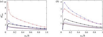
The fluctuation intensities of the perturbation fluxes in (3.15) are represented in figure 1 as lines with symbols. They are weaker than the values cited above for the fluxes based on the full velocities, and only the standard deviation of
 $R_{11}^{\prime +}$
reaches
 $O(10)$
near the wall. However, it should be borne in mind that these fluxes no longer represent the full momentum transfer, and that part of the momentum is now carried by the linear advection terms on the right-hand side of (3.14). The leftmost one,
 $U\unicode[STIX]{x2202}_{1}u_{1}^{\prime }$
, is the advection of the velocity fluctuations by the mean velocity profile, and appears as flux fluctuations in any but the semi-Lagrangian frame of reference that follows the mean flow. It was shown in Jiménez (Reference Jiménez2013a
) that approximately 90 % of the particle acceleration in a channel flow is due to this term, and this is the main reason why the standard deviation of the fluxes is reduced when defined in terms of fluctuations. The price of this non-uniform frame of reference is the last term on the right-hand side of (3.14),
 $u_{2}^{\prime }\unicode[STIX]{x2202}_{2}U$
, which is the classical lift-up representing the change in mean velocity of a fluid particle as it moves with respect to the wall. Whether these transfers should be treated as fluxes or sources has to be decided on physical grounds.
4 Results
The results of applying the optimisation process to (3.14) are shown in figure 1, where they are compared with the classical algebraic perturbation fluxes
 $R_{ij}^{\prime }$
. The optimisation reduces the fluctuating intensity of all the fluxes by a substantial factor that varies among components. In fact, the reduction is larger than shown in the figure, because the standard deviation is computed with respect to the mean value, which is typically not zero for the classical fluxes. For example,
 $\langle R_{11}^{\prime }\rangle =\langle {u_{1}^{\prime }}^{2}\rangle \geqslant 0$
, while it follows from (2.10) that the mean value of the optimal diagonal fluxes along any homogeneous direction vanishes identically. All the optimal flux fluctuations are of similar magnitude, and of the order of the mean momentum transfer rate,
 $u_{\unicode[STIX]{x1D70F}}^{2}$
. Note that the standard deviations discussed here refer to the fluctuations of the quadratic functions of the velocities, as in
 $(u^{2})_{rms}^{2}=\langle u^{4}\rangle -\langle u^{2}\rangle ^{2}$
, not to those of the velocities themselves.
Although not shown in figure 1, the effect of the pressure on the diagonal stresses
 $R_{ii}^{\prime }$
in (3.15) (no summation implied) is not negligible, and always increases the fluctuation intensities when compared with the Reynolds products
 ${u_{i}^{\prime }}^{2}$
. This is particularly evident for the wall-normal velocity
 $u_{2}^{2}$
. On the other hand, the effect of the viscous term in
 $R_{ij}^{\prime }$
is negligible above
 $x_{2}^{+}\approx 20$
.
Root-mean-squared fluctuation intensities of the momentum fluxes along the three coordinate directions, computed with the fluctuation velocity equation (3.14). (a) Fluxes of the streamwise momentum: – – –,
 $\unicode[STIX]{x1D719}_{11}$
; ——,
 $\unicode[STIX]{x1D719}_{12}$
; – ⋅ – ⋅ –,
 $\unicode[STIX]{x1D719}_{13}$
. (b) Fluxes of the transverse momenta: – – –,
 $\unicode[STIX]{x1D719}_{22}$
; ——,
 $\unicode[STIX]{x1D719}_{23}$
; – ⋅ – ⋅ –,
 $\unicode[STIX]{x1D719}_{33}$
. Lines with circles are
 $R_{ij}^{\prime }$
from (3.14). Those without symbols are optimum fluxes
 $\unicode[STIX]{x1D719}_{ij}^{\prime }$
from (3.5)–(3.10).

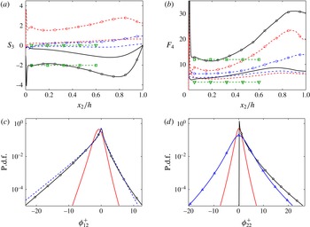
Higher-order moments of the fluctuation intensities of the centred momentum fluxes, computed from the fluctuation velocities: – – –,
 $\unicode[STIX]{x1D719}_{11}^{\prime }$
; ——,
 $\unicode[STIX]{x1D719}_{12}^{\prime }$
; – ⋅ – ⋅ –,
 $\unicode[STIX]{x1D719}_{22}^{\prime }$
. (a) Third-order skewness,
 $\langle \unicode[STIX]{x1D719}^{\prime 3}\rangle /\langle \unicode[STIX]{x1D719}^{\prime 2}\rangle ^{3/2}$
. (b) Fourth-order flatness,
 $\langle \unicode[STIX]{x1D719}^{\prime 4}\rangle /\langle \unicode[STIX]{x1D719}^{\prime 2}\rangle ^{2}$
. The horizontal dashed lines are theoretical values for different functions of Gaussian-distributed variables: ▿, a Gaussian variable
 $(S_{3}=0,~F_{4}=3)$
; ▫, the product of two Gaussian variables with cross-correlation coefficient
 $-0.4$
 $(S_{3}=-2.02,~F_{4}=11.9)$
. (c) Probability density function of
 $\unicode[STIX]{x1D719}_{12}$
at
 $x_{2}/h\in (0.1-0.2)$
, normalised in wall units. The dashed line is the product of two Gaussian variables with cross-correlation coefficient
 $-0.4$
. (d) As in (c), for
 $\unicode[STIX]{x1D719}_{22}$
. The line with triangles is for
 $u_{2}^{\prime 2}+p$
. In all panels, lines with circles are the Reynolds products,
 $u_{i}^{\prime }u_{j}^{\prime }$
, and those without symbols are optimum fluxes from (3.5)–(3.10).

The optimal fluxes are also less intermittent than the classical algebraic ones or than the Reynolds products
 $\unicode[STIX]{x1D70F}_{ij}=u_{i}^{\prime }u_{j}^{\prime }$
. Their third-order skewness and fourth-order flatness are given in figure 2(a,b). It is well known that the Reynolds products are skewed and intermittent, which is clear from the figure, but this is mostly a consequence of their definition as quadratic forms. For example, even if a variable is Gaussian distributed, its square is not, and Antonia & Atkinson (Reference Antonia and Atkinson1973) and Lu & Willmarth (Reference Lu and Willmarth1973) showed that the probability distribution of the product
 $u_{1}^{\prime }u_{2}^{\prime }$
is essentially the same as the product of two Gaussian variables with the correct cross-correlation coefficient. The theoretical moments for this product of Gaussian variables are given in figure 2(a,b), and represent well the observations for the tangential Reynolds product, except very near to and far from the wall. The optimal fluxes, which do not suffer from these algebraic artefacts, are much less intermittent and stay approximately Gaussian except in the buffer layer. Although not shown in figure 2 to avoid clutter, the effect of the pressure on
 $R_{ij}^{\prime }$
is to decrease intermittency. Particularly for
 $u_{2}^{\prime 2}$
and
 $u_{3}^{\prime 2}$
, the flatness of the Reynolds products is approximately three times higher than for the corresponding
 $R_{ii}^{\prime }=u_{i}^{\prime 2}+p-2\unicode[STIX]{x1D708}\unicode[STIX]{x2202}_{i}u_{i}^{\prime }$
(no summation). The effect of the viscous term is also negligible in this case.
The probability density functions (p.d.f.s) for two flux components in the ‘logarithmic’ layer are given in figure 2(c,d), where both the smaller standard deviation and the weaker intermittency are clear. In the case of
 $\unicode[STIX]{x1D70F}_{12}$
in figure 2(c), also shown is the theoretical p.d.f. for the product of two Gaussian variables, which fits the classical Reynolds product well except at the extreme tails. Note that the mean value of these two p.d.f.s is exactly the same,
 $\langle \unicode[STIX]{x1D719}_{12}^{+}\rangle =x_{2}/h-1$
, but is achieved by the two fluxes in different ways. While the p.d.f. of the classical Reynolds product peaks at
 $\unicode[STIX]{x1D70F}_{12}=0$
, and owes its negative mean value to the skewness of its tails, the distribution of the optimal fluxes is roughly symmetric about its mean value. Consequently, the volume fraction of the ‘countergradient’ momentum flux, defined as
 $\unicode[STIX]{x1D719}_{12}\unicode[STIX]{x2202}_{2}U>0$
, is approximately 15 % for the optimal fluxes
 $\unicode[STIX]{x1D719}_{12}^{\prime }$
in the logarithmic layer, and 30 % for
 $\unicode[STIX]{x1D70F}_{12}\approx R_{12}^{\prime }$
.
Figure 2(d) displays the p.d.f. of the diagonal stress
 $\unicode[STIX]{x1D719}_{22}$
. It also shows the narrower distribution of the optimal flux and its narrower tails, although the main difference in this case is that the classical product,
 $u_{2}^{\prime 2}$
, is intrinsically positive. Figure 2(d) also shows the effect of the pressure, discussed at the beginning of this section. Its main effect is to restore the approximate symmetry of the p.d.f. of
 $u_{2}^{\prime 2}+p$
, which now includes negative values. As mentioned above, this also decreases intermittency, although figure 2(d) shows that most of the decrease is due to the effect of centring the one-sided p.d.f. of the square. On the other hand, there is almost no difference between the p.d.f. of the optimum
 $\unicode[STIX]{x1D719}_{22}^{\prime }$
and that of its traceless equivalent,
 $\unicode[STIX]{x1D719}_{22}^{\prime }-\unicode[STIX]{x1D6F1}^{\prime }/3$
(not shown).
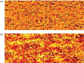
Wall-parallel snapshots of the instantaneous tangential momentum flux in a channel at
 $Re_{\unicode[STIX]{x1D70F}}=934$
(del Álamo et al.
Reference del Álamo, Jiménez, Zandonade and Moser2004) and
 $x_{2}/h=0.15$
. Flow is from left to right, and the area in the panels is
 $L_{1}\times L_{3}=4\unicode[STIX]{x03C0}h\times 3\unicode[STIX]{x03C0}h/2$
. (a) Classical flux
 $R_{12}^{\prime }$
from (3.15). (b) Optimal flux
 $\unicode[STIX]{x1D719}_{12}^{\prime }$
. In both cases, the flux is centred with its mean value, and the colour scale spans
 $\pm 3$
standard deviations, increasing from dark to light.

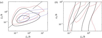
(a) Two-dimensional premultiplied spectra as functions of the wall-parallel wavelengths,
 $\unicode[STIX]{x1D701}=2\unicode[STIX]{x03C0}/\unicode[STIX]{x1D6FC}$
: ——,
 $R_{12}^{\prime }$
; – – –, optimal
 $\unicode[STIX]{x1D719}_{12}^{\prime }$
; – ⋅ – ⋅ –, cospectrum of
 $u_{1}^{\prime }$
and
 $u_{2}^{\prime }$
. The two contours contain 30 % and 80 % of the spectral mass. The dashed diagonals are
 $\unicode[STIX]{x1D701}_{1}=\unicode[STIX]{x1D701}_{3}$
. Flow as in figure 3,
 $x_{2}/h=0.15$
. (b) Streamwise premultiplied spectra as a function of
 $x_{2}$
: ——,
 $R_{12}^{\prime }$
; – – –,
 $\unicode[STIX]{x1D719}_{12}^{\prime }$
. Each horizontal section is a spectrum normalised to unit energy, and the contours are 50 % and 80 % of the global maximum. The dashed diagonal is
 $\unicode[STIX]{x1D701}_{1}=1.2\,x_{2}$
.

Reynolds and optimal fluxes are also structurally quite different. This is shown in figure 3(a,b), where the classical transverse Reynolds stress
 $R_{12}^{\prime }\approx u_{1}^{\prime }u_{2}^{\prime }$
is compared with the corresponding optimal flux
 $\unicode[STIX]{x1D719}_{12}^{\prime }$
. Both quantities are shown centred with respect to their mean and normalised with their standard deviation. This scaling absorbs the difference in their magnitude, but the geometry of the field remains different. This is partly because of the stronger intermittency of
 $R_{12}^{\prime }$
, manifested by the presence of numerous dark and light spots in figure 3(a), but the characteristic streamwise organisation of the Reynolds stresses is also much less marked in the optimal flux in figure 3(b). The differences are even more marked in the buffer layer (not shown), where the classical tangential Reynolds stress reflects the organisation of the near-wall velocity streaks, while the optimal one does not. The correlation coefficient between
 $R_{12}^{\prime }$
and
 $\unicode[STIX]{x1D719}_{12}^{\prime }$
is approximately 0.5 throughout most of the channel, but falls to approximately 0.1 at
 $x_{2}^{+}\approx 15$
.
The differences are confirmed by the spectra in figure 4, where
 $\unicode[STIX]{x1D719}_{12}^{\prime }$
is compared to
 $R_{12}^{\prime }$
. They are presented premultiplied by the appropriate wavenumbers, and displayed in terms of the wavelengths
 $\unicode[STIX]{x1D701}_{j}=2\unicode[STIX]{x03C0}/\unicode[STIX]{x1D6FC}_{j}$
. Note that these spectra, such as
 $E_{RR}=\langle \widehat{R}_{12}^{\prime }\widehat{R}_{12}^{\prime }\rangle$
, are different from the cospectrum,
 $E_{12}=-\langle \widehat{u}_{1}^{\prime }\widehat{u}_{2}^{\prime }\rangle$
, which is included in figure 4(a) for comparison. The latter represents the spectral contribution of the product
 $\unicode[STIX]{x1D70F}_{12}=u_{1}^{\prime }u_{2}^{\prime }$
to the mean tangential stress, while the former reflects the geometry of the product (Lozano-Durán et al.
Reference Lozano-Durán, Flores and Jiménez2012), and expresses the spectral contribution to the variance. Figure 3(a) shows two-dimensional spectra in the plane
 $x_{2}/h=0.15$
, and reveals that the cospectrum is contaminated by the elongated streaks of the streamwise velocity. In the case of products of velocities, the high-order spectra such as
 $E_{RR}$
were shown by Van Atta & Wyngaard (Reference Van Atta and Wyngaard1975) to be dominated by the sweeping of the small scales by the larger ones, and the spectrum of
 $R_{12}^{\prime }$
is also anisotropic, although less than the cospectrum. On the other hand, the spectrum of
 $\unicode[STIX]{x1D719}_{12}^{\prime }$
, which is only indirectly linked to
 $u_{1}$
through the right-hand side of (3.14), is weakly influenced by the elongated streaks, and is more isotropic (i.e. closer to
 $\unicode[STIX]{x1D701}_{1}=\unicode[STIX]{x1D701}_{3}$
).
Figure 4(b) shows one-dimensional premultiplied spectra as functions of the streamwise wavelength and of the distance to the wall. It is known that the wavelength of the maximum of the cospectrum increases linearly with
 $x_{2}$
at high Reynolds numbers (see figure 1b in Jiménez Reference Jiménez2012), but this is still not obvious at the relatively low Reynolds number of figure 4. The reason is that
 $R_{12}^{\prime }$
is dominated by the effect of the wall-parallel velocity
 $u_{1}^{\prime }$
, whose scale is not constrained by the impermeability condition near the wall (Townsend Reference Townsend1961). On the other hand, figure 4(b) shows that the spectral peak of
 $\unicode[STIX]{x1D719}_{12}^{\prime }$
, which is free from the spurious influence of the inactive wall-parallel motions, grows linearly away from the wall even at this relatively low Reynolds number. It can be shown that the difference between the spectrum of classical and optimal fluxes is largest in the buffer layer, and decreases with increasing distance to the wall. This effect is more marked for quantities involving
 $u_{1}^{\prime }$
or
 $u_{3}^{\prime }$
, and almost non-existent for
 $\unicode[STIX]{x1D719}_{22}^{\prime }$
.
5 Discussion and conclusions
We have noted that the fluxes implicit in conservation laws are not uniquely defined, in a way similar to the gauge ambiguity of classical field theory. As an example, we have developed a particular definition that minimises the integral of their square. Although this definition should not be considered in any way unique, it has the intuitive appeal of minimising ‘sterile circularities’ in the transfers of conserved scalars. We have generalised these observations to vector conservation laws and tensor fluxes, and presented a way to compute such fluxes from simulations. We have applied it to the momentum transfer in turbulent channels, and showed that the results differ substantially from the classical Reynolds stresses. In particular, the fluctuations of the optimal fluxes are weaker than the classical ones, their probability distributions are closer to Gaussian, and their spectra show less contamination from individual velocity components.
These results raise some interesting questions that go beyond the scope of the present paper, and which should eventually be considered individually. Not the least of them is whether, given their arbitrariness, pointwise Reynolds stresses should be considered to be proper targets for the subgrid models of LES. Only their divergence is important, while the stresses themselves can vary widely without ill effects. This may help explain the apparent contradiction that a priori testing of many LES models fails grossly while the a posteriori results are reasonable (Bardina Reference Bardina1983). It is interesting to note in this context that the very successful dynamic model of Germano et al. (Reference Germano, Piomelli, Moin and Cabot1991) can be characterised as an algorithm to determine the magnitude of the eddy viscosity from the difference of the subgrid stresses at two different scales, and can therefore be seen as an integral implementation of fitting the divergence of the fluxes in scale space, rather than the fluxes themselves.
In particular, we noted in the introduction that, while gauge transformations leave the field equations invariant, the same is not generally true when the equations are written in terms of the fluxes or of the potentials, and remarked that this may give rise to problems in the second-order turbulence closures that model the Reynolds stresses directly. While there should be nothing wrong with their use in applications to domains large enough for the flow to be considered in equilibrium, the results in this paper suggest that they may not be very useful over smaller domains, such as over individual LES cells. In fact, Lund & Novikov (Reference Lund and Novikov1993) showed that introducing a full set of tensor invariants in models of the subgrid stresses did not improve them appreciably with respect to simpler models. On the other hand, the above results suggest that much of the effort spent in modelling individual components may be largely irrelevant, as long as the divergence of the flux is correctly represented. For example, there is probably no reason why closures should be expected to reproduce the intermittency of the Reynolds stresses. Note that this conclusion applies to all gauges, including the optimal one discussed here. The present paper should not be construed as an invitation to model the optimal fluxes, but as an indication that it is enough for closures to mimic the simplest tensor structure that guarantees the right divergence, even if the fluxes themselves appear to be incorrect. Although the formulation of turbulence models is beyond the scope of this paper, it is interesting to note that the expression (2.10) of the optimal fluxes as the symmetrised gradient of a vector suggests the possibility of formulations that depend on fewer than full tensor quantities.
The somewhat different approach of simplifying second-order closures by modelling directly the divergence of the stress tensor (the ‘turbulent force’), instead of the tensor itself, has been discussed before by Perot & Moin (Reference Perot and Moin1996), following earlier work by Wu, Zhou & Wu (Reference Wu, Zhou and Wu1996) and Wu et al. (Reference Wu, Zhou, Lu and Fan1999). This last paper, which also frames the problem in terms of the gauge ambiguity of the stress tensor, contains references to earlier work in the same direction.
The gauge freedom in the definition of the momentum fluxes also calls into question the meaning of individual structures of intense Reynolds products, such as those studied in the classical ‘quadrant’ classification of the
 $(u_{1}^{\prime },u_{2}^{\prime })$
plane by Wallace et al. (Reference Wallace, Eckelmann and Brodkey1972) and Lu & Willmarth (Reference Lu and Willmarth1973), and in modern three-dimensional extensions of the same idea by Lozano-Durán et al. (Reference Lozano-Durán, Flores and Jiménez2012) and Lozano-Durán & Jiménez (Reference Lozano-Durán and Jiménez2014). Although a detailed investigation of this question is beyond the scope of this paper, the present results suggest that these structural analyses should be repeated using other gauges, such as the present optimal one, to test how dependent on the gauge are the properties of the resulting structures. This is a case in which intermittency is beneficial, since the hope is to identify structures strong enough to stay coherent independently of the rest of the flow, but able to explain some flow characteristics from a small fraction of the total volume. The weaker intermittency of the optimal fluxes in figure 2 suggests that analyses based on intense structures may be less relevant for them than for the classical Reynolds products. For example, it follows from the p.d.f.s in figure 2(c) that, while the 10 % strongest points of
 $-\unicode[STIX]{x1D70F}_{12}$
contain approximately 70 % of the total Reynolds stress, the equivalent strongest 10 % of the optimal
 $-\unicode[STIX]{x1D719}_{12}^{\prime }$
accounts for only 33 %.
Also interesting is that (1.2) and (1.3) provide an algorithmic ‘accounting’ definition of fluxes that can be computed even in cases in which the physical formulation is difficult to interpret locally. There is no implication that the result can be expressed in terms of a ‘formula’ of local observables, but this is no worse than for the pressure, which is part of the classical momentum and energy fluxes, and can only be determined as the solution of an elliptic partial differential equation. Numerically, all variables are equally simple to obtain, particularly since (1.3) ensures that the knowledge of any expression for the fluxes provides a way to compute all other representations.
For example, the Kolmogorov inertial energy cascade assumes that energy is transferred across scales from its injection into large structures to its dissipation in small viscous ones. The momentum transfer in physical space and the energy cascade in wavenumber space are different problems, but the underlying mathematical ambiguity is the same, and the questions of how relevant are intermittency and backscatter are similar. Defining the energy flux,
 $\unicode[STIX]{x1D700}$
, is straightforward in isotropic flows for which scale is a one-dimensional parameter and the conservation equation (1.2) can be solved by a simple quadrature. In more general situations, the definition is no longer unique. Even in the simple case of statistically isotropic flows, the energy flux in three-dimensional wavenumber space is a vector that depends on the wavenumber and time. It only coincides with the classical scalar
 $\unicode[STIX]{x1D700}$
when averaged over full spherical wavenumber shells.
In the slightly more complicated case of statistically homogeneous anisotropic shear turbulence, the average energy flux is also a vector in wavenumber space, but its direction is undetermined even in the mean. Any attempt to write energy conservation in spectral space in terms of observables leads to wavenumber triads that cannot be interpreted locally (Kraichnan Reference Kraichnan1971). The formulation in Dar, Verma & Eswaran (Reference Dar, Verma and Eswaran2001) shows that triads can be combined to provide an essentially unique definition for the energy transfer among arbitrary modes, but the fundamental transfer unit is still the triad (Verma Reference Verma2004). Even this formulation does not provide a transfer definition restricted to contiguous wavenumbers. Energy is transferred among all possible mode pairs in wave space, and it is interesting that these authors note that there is an undetermined ‘circulating transfer’ in any triad that is essentially a gauge (Verma Reference Verma2004). Most of these ambiguities disappear when the energy flux is averaged over sufficiently large wavenumber surfaces, or over time, but, when applied locally, they are at the root of many of the discussions about the instantaneous direction of the energy transfer and about the relevance of backscatter (Domaradzki & Rogallo Reference Domaradzki and Rogallo1990). An energy equation equivalent to (1.2) in wavenumber space provides a definition of a vector energy transfer rate that is local, algorithmically computable and, inasmuch as energy conservation embodies the behaviour of the energy in spectral space, as physically ‘relevant’ as any definition based on algebraic expressions. Note that even the classical one-dimensional definition of
 $\unicode[STIX]{x1D700}$
relies on a homogeneous boundary condition such as (2.4); the energy transfer rate can only be given a definite value by assuming that it vanishes at very large and at very small scales.
An even more interesting application concerns non-homogeneous flows. While the concept of scale is unambiguous in homogeneous flows, it is harder to define in inhomogeneous ones, where it is not easily separated from position. Consider, for example, a turbulent channel in which energy is being transferred among eddies of different sizes while they move relative to the wall. The ambiguity is whether their energy should be considered as transferred across space or across scale. A recent analysis of this problem led to a transport equation for the second-order structure function (the ‘scale energy’) in the form of a double divergence, in space and scale, of a six-dimensional vector flux (Hill Reference Hill2002),
 $$\begin{eqnarray}\unicode[STIX]{x2202}_{x_{j}}\unicode[STIX]{x1D719}_{j}+\unicode[STIX]{x2202}_{r_{j}}\unicode[STIX]{x1D713}_{j}=S,\end{eqnarray}$$
where
 $x_{j}$
with
 $j=1,\ldots ,3$
represent the spatial directions, and
 $r_{j}$
are the respective separations along those directions. The analysis provides explicit expressions for the fluxes in space,
 $\unicode[STIX]{x1D719}_{j}$
, and scale,
 $\unicode[STIX]{x1D713}_{j}$
, which have been computed and interpreted in turbulent channels by Cimarelli & De Angelis (Reference Cimarelli and De Angelis2011, Reference Cimarelli and De Angelis2012). They are not optimal in the sense described here (Cimarelli, private communication). Irrespective of the merits of the structure function as a measure of energy at a given scale, the previous considerations show that these fluxes and this analysis are not unique, and suggest that their conclusions should be revisited in terms of their robustness with regards to the different definitions.
In general, cascade theories concern themselves with fluxes, which are typically conserved across some ‘inertial’ range. The quantities being transferred, such as the energy, are typically created and dissipated somewhere else in the system. The results in the present paper suggest that the concept of flux, and therefore of cascades, should be re-examined with care.
Acknowledgements
This work was supported by the European Research Council Coturb grant ERC-2014.AdG-669505. I am grateful to the Sidney Sussex College and to the Department of Engineering of the University of Cambridge for their hospitality during the preparation of the manuscript.