


1. Introduction
The Richardson–Kolmogorov view of energy cascade (Kolmogorov Reference Kolmogorov1941a,Reference Kolmogorovb,Reference Kolmogorovc) is central to the classical phenomenology of turbulent flows, whose significance cannot be overemphasized. It is well known that a priori hypotheses formulated by Kolmogorov (i.e. local isotropy, first similarity and second similarity hypotheses) have to be invoked to derive the  $-5/3$ power law for energy spectra in the so-called ‘inertial range’. However, the deduction from Kolmogorov's hypotheses has no direct connection to the Navier–Stokes equations. More specifically, the most common way to derive the
 $-5/3$ power law is dimensional analysis.
The earliest attempt to explore energy cascade based on the Navier–Stokes equations was performed by Kármán and Howarth (Pope Reference Pope2000). The Kármán–Howarth equation predicts the four-fifths law of the third-order structure function, which is viewed as ‘one of the few exact, but non-trivial, results in the statistical theory of isotropic turbulence’ (Davidson Reference Davidson2004). The Kármán–Howarth equation offers the second way to derive the  $-5/3$ power law if we further assume that the skewness factor of the velocity differences is constant within the inertial range (Kolmogorov Reference Kolmogorov1941a).
It should be stressed that several hypotheses (i.e. homogeneous and isotropic) are necessary for the derivation of the Kármán–Howarth equation, albeit compared with the  $-5/3$ power law fewer hypotheses are required. The Kármán–Howarth–Monin–Hill (KHMH) equation, which is directly derived from Navier–Stokes equations (Pope Reference Pope2000) without resorting to any assumptions, on the other hand, allows us to explore the scale-by-scale energy transfer in any kind of incompressible flow (Marati, Casciola & Piva Reference Marati, Casciola and Piva2004; Gomes-Fernandes, Ganapathisubramani & Vassilicos Reference Gomes-Fernandes, Ganapathisubramani and Vassilicos2015; Valente & Vassilicos Reference Valente and Vassilicos2015; Portela, Papadakis & Vassilicos Reference Portela, Papadakis and Vassilicos2017; Yasuda & Vassilicos Reference Yasuda and Vassilicos2018). Therefore, the KHMH equation is also viewed as the generalized Kármán–Howarth equation.
The  $-5/3$ energy spectra, probably the most remarkable deduction from Kolmogorov phenomenology, have already received considerable experimental and numerical support (e.g. Goto (Reference Goto2012) and references therein). Recently, however, new evidences (Laizet, Vassilicos & Cambon Reference Laizet, Vassilicos and Cambon2013; Gomes-Fernandes, Ganapathisubramani & Vassilicos Reference Gomes-Fernandes, Ganapathisubramani and Vassilicos2014; Hearst & Lavoie Reference Hearst and Lavoie2014; Isaza, Salazar & Warhaft Reference Isaza, Salazar and Warhaft2014; Laizet, Nedić & Vassilicos Reference Laizet, Nedić and Vassilicos2015; Zhou et al. Reference Zhou, Nagata, Sakai, Ito and Hayase2016; Nagata et al. Reference Nagata, Saiki, Sakai, Ito and Iwano2017; Paul, Papadakis & Vassilicos Reference Paul, Papadakis and Vassilicos2017; Portela et al. Reference Portela, Papadakis and Vassilicos2017), both experimental and numerical, have emerged that the
 $-5/3$ energy spectra can be found in the turbulent region where Kolmogorov's hypotheses do not hold (also named non-Kolmogorov
 $-5/3$ spectra). The first ever investigation focusing on the spatial origin of the
 $-5/3$ energy spectra was carried out by Laizet et al. (Reference Laizet, Vassilicos and Cambon2013, Reference Laizet, Nedić and Vassilicos2015) in spatially developing turbulent flows generated by fractal grids. Since then there has been a multitude of studies of various kinds of turbulent flows on this subject. Portela et al. (Reference Portela, Papadakis and Vassilicos2017) reported that in the near field of a square prism, where the flow is highly inhomogeneous and anisotropic, a well-defined energy spectrum with an exponent close to
 $-5/3$ can be observed. Similar findings have also been reported in uniformly sheared flows (Nedić & Tavoularis Reference Nedić and Tavoularis2016), grid-generated turbulence (by single square (Laizet et al. Reference Laizet, Nedić and Vassilicos2015; Melina, Bruce & Vassilicos Reference Melina, Bruce and Vassilicos2016; Zhou et al. Reference Zhou, Nagata, Sakai, Ito and Hayase2016; Paul et al. Reference Paul, Papadakis and Vassilicos2017), regular (Isaza et al. Reference Isaza, Salazar and Warhaft2014) and fractal (Laizet et al. Reference Laizet, Vassilicos and Cambon2013; Gomes-Fernandes et al. Reference Gomes-Fernandes, Ganapathisubramani and Vassilicos2014; Nagata et al. Reference Nagata, Saiki, Sakai, Ito and Iwano2017) grids), dual-wake flow (Zhou et al. Reference Zhou, Nagata, Sakai and Watanabe2019) and dual-jet flow (Zhou et al. Reference Zhou, Nagata, Sakai and Watanabe2018). The results of the aforementioned investigations all suggested that even in the turbulent regions where the Reynolds number is considerably small and the flow is highly inhomogeneous and anisotropic, a well-defined
 $-5/3$ energy spectrum can still be found.
Another equally important but less noticed finding is that the occurrence of the extended range of the  $-5/3$ energy spectra appears to be intimately associated with extreme/intermittent events (Laizet et al. Reference Laizet, Nedić and Vassilicos2015; Melina et al. Reference Melina, Bruce and Vassilicos2016; Paul et al. Reference Paul, Papadakis and Vassilicos2017). The term ‘extreme events’ is used rather loosely here to indicate that the corresponding velocity fluctuations are remarkably non-Gaussian distributed with a high probability of occurrence of rare events (i.e. large magnitude of velocity fluctuations). In our previous study on dual-wake flows (Zhou et al. Reference Zhou, Nagata, Sakai and Watanabe2019), the physical mechanism responsible for the extreme events was suggested to be attributed to large-scale vortex streets. It has been demonstrated that at in the upstream region (i.e.
 $X/T_0=6$), where the flow field is in a state of transition and is not fully developed, the range of the
 $-5/3$ power law appears to be determined by two different turbulence behaviours, one being large-scale vortex shedding, which defines the lower frequency part of the
 $-5/3$ power law, and the other being the burst of intermittent fluctuations, which defines the higher frequency part of the
 $-5/3$ power law. Here,
 $X$ is the streamwise distance from the cylinder and
 $T_0$ is the thickness of the square cylinder. Furthermore, in the upstream region of the dual-wake flow, where the celebrated
 $-5/3$ energy spectrum appears, the expected
 $2/3$ power law of the second-order structure function in physical space is absent. Instead, the returned power-law exponent is
 $1$, which is much larger than
 $2/3$. Therefore, the spectrum with
 $-5/3$ power-law shape found at
 $X/T_0=6$ is regarded as a ‘non-Kolmogorov’
 $-5/3$ spectrum. This large power-law exponent reflects a significant non-locality (i.e. direct interaction of large-scale vortex shedding and small-scale motions). With downstream distance the strength of the large-scale vortex shedding decreases and the expected 2/3 power law emerges at
 $X/T_0=26$. Moreover, the downstream flow field becomes more or less homogeneous and isotropic. In view of this, to some extent the corresponding spectrum can be viewed as a ‘quasi-Kolmogorov’
 $-5/3$ spectrum. It should be emphasized that the term ‘quasi-Kolmogorov’ used does not further imply whether the local energy cascade process is equilibrium or not. The corresponding energy transfer mechanisms (both one-point and two-point energy balances) at
 $X/T_0=6$ and
 $26$ are still unclear.
Recently, energy cascade processes in physical space in various kinds of flows (e.g. wall turbulence (Marati et al. Reference Marati, Casciola and Piva2004), grid-generated turbulence (Gomes-Fernandes et al. Reference Gomes-Fernandes, Ganapathisubramani and Vassilicos2014; Valente & Vassilicos Reference Valente and Vassilicos2015), single-wake flows (Portela et al. Reference Portela, Papadakis and Vassilicos2017) and homogeneous isotropic turbulence (Yasuda & Vassilicos Reference Yasuda and Vassilicos2018)) have been reported. It might be worth mentioning the aforementioned studies mainly focused on fully turbulent flow fields. For example, Portela et al. (Reference Portela, Papadakis and Vassilicos2017) numerically explored the turbulence cascade inside the near wake behind a single square cylinder. In this work, however, of particular interest is the scale-by-scale energy transfer at the upstream location  $X/T_0=6$, where the turbulent flow is highly intermittent (i.e. composed of both laminar large-scale oscillations and strong turbulent fluctuations). To clarify the effects of the pronounced large-scale oscillations at
 $X/T_0=6$ on the energy cascade, the scale-by-scale energy transfer over long separation ranges comparable to the size of large-scale vortex shedding is investigated. Moreover, a comparison of the energy transfer mechanisms (both one-point and two-point energy transfer) at
 $X/T_0=6$ and
 $26$ certainly contributes to a more complete picture of the so-called ‘non-Kolmogorov’ and ‘quasi-Kolmogorov’
 $-5/3$ energy cascade.
Besides the theoretical importance as mentioned above, wake interactions are also encountered in various engineering situations (e.g. wind turbines, bridges, buildings and heat exchanger tubes). Over the past few decades, various kinds of experiments using laser Doppler velocimetry (Kolář, Lyn & Rodi Reference Kolář, Lyn and Rodi1997), hot-wire probe (Alam, Zhou & Wang Reference Alam, Zhou and Wang2011), laser-induced fluorescence (Alam & Zhou Reference Alam and Zhou2013) and particle imaging velocimetry (Alam, Bai & Zhou Reference Alam, Bai and Zhou2016) have been carried out to study the turbulent flow behind two side-by-side square cylinders. However, except for our previous numerical study (Zhou et al. Reference Zhou, Nagata, Sakai and Watanabe2019) there have been very few direct numerical simulations (DNSs) of dual-wake flow.
The main object of this paper is to complement our previous study of spatially developing dual-wake flow by investigating the one-point and two-point turbulent kinetic energy budgets. The remaining parts of the paper are as follows. In § 2, we present the simulation set-up along with the geometric details. The spatial evolution of the centreline intermittency factor and the conditional statistics are presented in § 3. In §§ 4 and 5, the one-point and two-point energy transfer processes at two selected locations (i.e.  $X/T_0=6$ and
 $26$) are numerically investigated. In § 6, our main results are summarized.
2. Numerical and geometric details
In this study, DNSs are performed to investigate the turbulent flow behind two side-by-side square cylinders, through which we could easily get access to the full velocity and pressure fields with high fidelity, which are the essential prerequisites for the investigation of the scale-by-scale cascade. It would be difficult, if not impossible, to access such flow information through experimental measurements. Hence, DNSs of turbulent flow due to two identical parallel square cylinders placed side-by-side are performed in this study. It is worth mentioning that in previous experimental studies of the process of energy cascade (Hearst & Lavoie Reference Hearst and Lavoie2014; Gomes-Fernandes et al. Reference Gomes-Fernandes, Ganapathisubramani and Vassilicos2015; Valente & Vassilicos Reference Valente and Vassilicos2015), several simplifying assumptions were made due to the difficulties of collecting the full velocity and pressure fields. On the other hand, by means of DNSs we can compute accurately all terms in the KHMH equation.
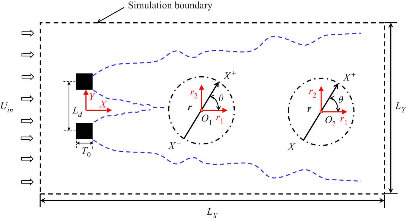
A schematic side view of the simulation domain along with the two kinds of coordinate systems (i.e.  $(x,y,z)$ and
 $(r_1,r_2,r_3)$) are presented in figure 1. The Cartesian coordinate system
 $(x,y,z)$ is adopted for numerical simulation and the origin of this system is placed at the midpoint of the two square cylinders. The coordinates
 $X$,
 $Y$ and
 $Z$ stand for the the streamwise, vertical and spanwise directions, respectively. The lengths
 $L_X$,
 $L_Y$ and
 $L_Z$ stand for the sizes of the computational domain in the streamwise, vertical and spanwise directions (i.e.
 $X$,
 $Y$ and
 $Z$ directions), respectively. The coordinates
 $(r_1,r_2,r_3)$ are employed to evaluate the interscale energy budget between the two points
 $X^+$ and
 $X^-$ in real space. The components
 $r_1$,
 $r_2$ and
 $r_3$ are evaluated along the streamwise (direction of the mean flow), vertical and spanwise directions, respectively. The position
 $\boldsymbol {x}$ of the centroid
 $O$ and the separation vector
 $\boldsymbol {r}$ are defined as
 $\boldsymbol {x}=(1/2)(\boldsymbol {X}^+ + \boldsymbol {X}^-)$ and
 $\boldsymbol {r} = \boldsymbol {X}^+ - \boldsymbol {X}^-$, respectively. In the following sections, two centroids located at
 $(X/T_0,Y/T_0)=(6,0)$ and
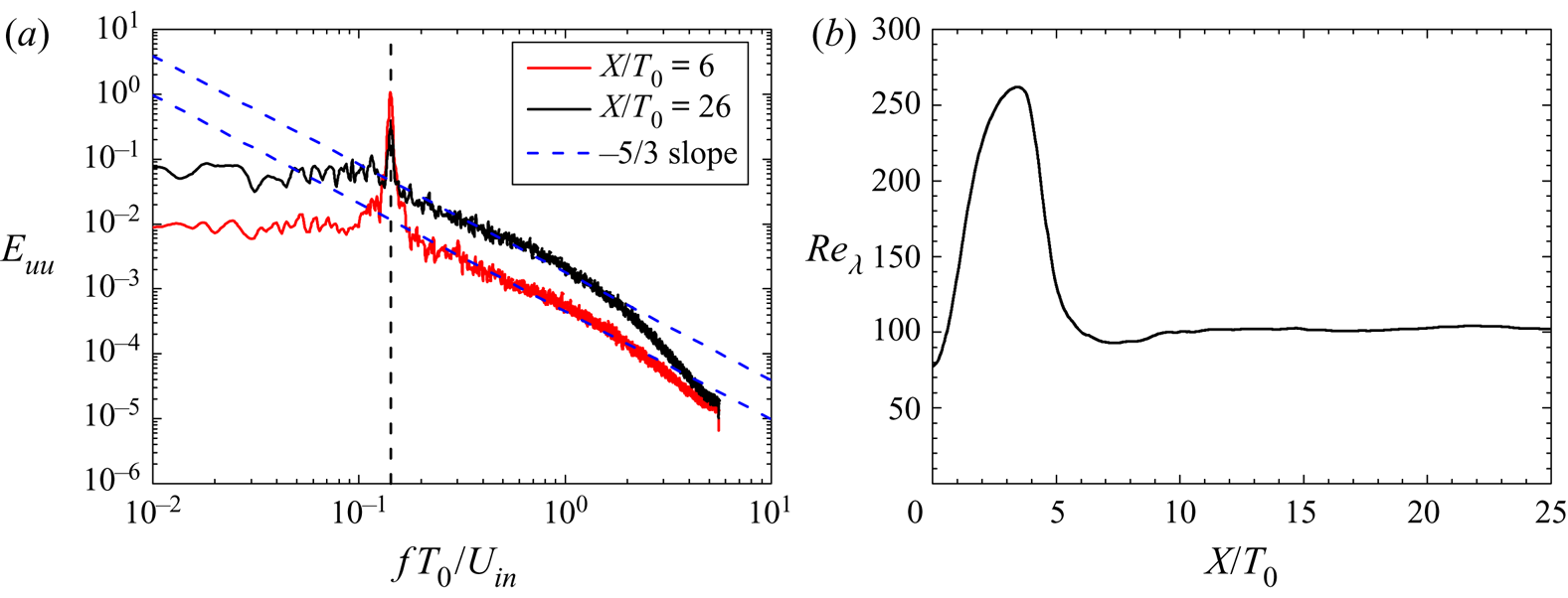
 $(26,0)$ are considered to investigate the interscale energy transfer in dual-wake flows by using KHMH equations. The spectra of the two centroids considered and the local Taylor length-scale-based Reynolds number
 $Re_{\lambda }$ (
 $=u_1\lambda /\nu$) with
 $\lambda ^2 = \langle u_1^{2}\rangle / \langle (\partial u_1 / \partial x)^{2}\rangle$ are shown in figures 2(a) and 2(b), respectively. It can be seen that
 $Re_{\lambda }$ remains roughly constant and is around 100 in the region
 $X/T_0 \ge 5$ (see figure 2b).
Definition of the two coordinate systems used in this study. The angle between the axis  $r_1$ and the vector
 $\boldsymbol {r}$ is defined as
 $\theta$. The notations
 $O_1$ and
 $O_2$ indicate the two centroids, namely
 $(X/T_0,Y/T_0) = (6, 0)$ and
 $(26, 0)$. The dashed lines represent the simulation boundaries. For simplicity, only the two-dimensional side view is plotted. The schematic drawing is not to scale.

 $(a)$ Energy spectra of the streamwise velocity fluctuations
 $u_1$ at
 $X/T_0 =6$ and 26 (Zhou et al. Reference Zhou, Nagata, Sakai and Watanabe2019).
 $(b)$ Streamwise evolution of the local Reynolds number
 $Re_{\lambda }$ along the centreline.

The computational and geometric details of this study are given in table 1. Here,  $Re_{T_0}$ is the inlet Reynolds number based on the inlet velocity
 $U_{in}$ and the thickness of square bar
 $T_0$. Length
 $L_d$ denotes the separation distance between the two cylinders. The two side-by-side square cylinders are placed at
 $X_{bar}/T_0=8$, with
 $X_{bar}$ being the streamwise distance from the inlet to the cylinders. Except for the domain size (i.e.
 $L_X \times L_Y \times L_Z=42 T_0 \times 38 T_0 \times 5 T_0$) and the corresponding mesh numbers (i.e.
 $N_X \times N_Y \times N_Z = 961 \times 874 \times 100$), the other numerical settings (e.g. inlet Reynolds number, streamwise location of the two square bars, boundary conditions) are exactly the same as those in Zhou et al. (Reference Zhou, Nagata, Sakai and Watanabe2019). A relatively small inlet Reynolds number
 $Re_{T_0}=2500$ is adopted to ensure sufficiently fine spatial resolution. It has been confirmed in Zhou et al. (Reference Zhou, Nagata, Sakai and Watanabe2019) that the streamwise evolution of the centreline resolution
 $(\Delta X \Delta Y \Delta Z)^{1/3}/\eta$ is always below 3.2, where
 $\Delta X$,
 $\Delta Y$ and
 $\Delta Z$ are the mesh sizes in the streamwise, vertical and spanwise directions, respectively, and
 $\eta$ is the Kolmogorov scale. The Strouhal number of the large-scale vortex shedding is
 $St = f_sT_0/U_{in} \simeq 0.142$ with
 $f_s$ being the vortex shedding frequency. The statistical results are averaged over
 $N_{total} = 400\,000$ time steps corresponding to approximately 250 vortex shedding cycles and the time step is
 $\Delta t /(T_0/U_{in}) = 0.0045$. The convergence of the high-order statistics (i.e. third order) in the KHMH equations, which is more demanding than other low-order statistics, will be discussed later.
Computational and geometric details.

In the  $X$ direction, a uniformly distributed inlet velocity
 $U_{in}$ is prescribed at the inlet (i.e.
 $X/T_0=-8$) and a convective outflow condition is adopted at the outlet (i.e.
 $X/T_0=34$). In the other two directions (i.e.
 $Y$ and
 $Z$ directions), the boundaries (i.e.
 $Y/T_0={\pm }19$ and
 $Z/T_0={\pm }2.5$) are set to be periodic. The modelling of the bluff square cylinders is based on the procedure proposed by Parnaudeau et al. (Reference Parnaudeau, Carlier, Heitz and Lamballais2008). The parallel finite difference solver ‘Incompact3d’ (Laizet & Lamballais Reference Laizet and Lamballais2009; Laizet, Lamballais & Vassilicos Reference Laizet, Lamballais and Vassilicos2010; Laizet & Li Reference Laizet and Li2011) is employed to solve the Navier–Stokes equations for incompressible flows with a constant kinematic viscosity. See Zhou et al. (Reference Zhou, Nagata, Sakai and Watanabe2019) for further numerical details along with the verification of the numerical strategies.
3. Flow visualization and intermittency
3.1. Flow visualization
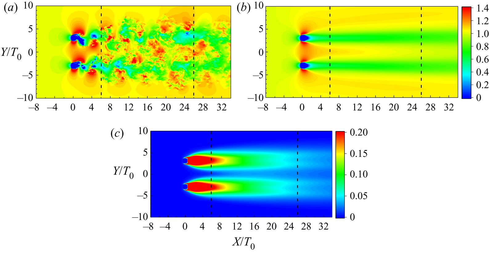
The instantaneous and mean streamwise velocity fields in the  $X\text {--}Y$ plane for the turbulent flow around two identical parallel square cylinders are shown in figure 3, along with the mean turbulent kinetic energy, in which only parts of the full simulation domain are plotted. Unless otherwise stated, the mean and fluctuating velocity components are denoted by upper case and lower case, respectively.
Contour plots of  $(a)$ the normalized instantaneous streamwise velocity field
 $(u_1+U_1)/U_{in}$,
 $(b)$ the normalized mean streamwise velocity field
 $U_1/U_{in}$ and
 $(c)$ the normalized kinetic energy
 $((U_{rms}^2+V_{rms}^2+W_{rms}^2)/U_{in}^2)/2$. For all maps, only a part of the flow fields (i.e.
 $-10 < Y/T_0 < 10$ in the vertical direction) is plotted. The two vertical dashed lines indicate
 $X/T_0=6$ and
 $26$, respectively.

The gap flow between the two cylinders is initially laminar. The transition to turbulent motion for the gap flow is evident from figure 3(a), which is introduced by the intermittent encounter of the two turbulent wakes. One can expect that the gap flow can be highly intermittent in the upstream region and will become fully turbulent in the far downstream region. A quantitative description of the intermittency is given below.
In the upstream region, the turbulent flow exhibits strong inhomogeneity in terms of the one-point statistics (i.e. mean streamwise velocity and turbulent kinetic energy) especially in the vertical direction. The highly inhomogeneous turbulent flow also suggests distinct anisotropy. With increasing distance, the inhomogeneities of the mean velocity and the turbulence intensities can be gradually smoothed out. However, even at the most downstream location considered (i.e.  $X/T_0=34$), the two wakes do not fully merge as hinted at by the persistence of the jet-like distribution of
 $U_1$ around the centreline (see figure 3b) and also the discernible large magnitudes of the turbulent kinetic energy of the two wakes (see figure 3c). As will be shown in the following section, the lack of homogeneity can exert a significant influence on both one-point and two-point energy transfer processes.
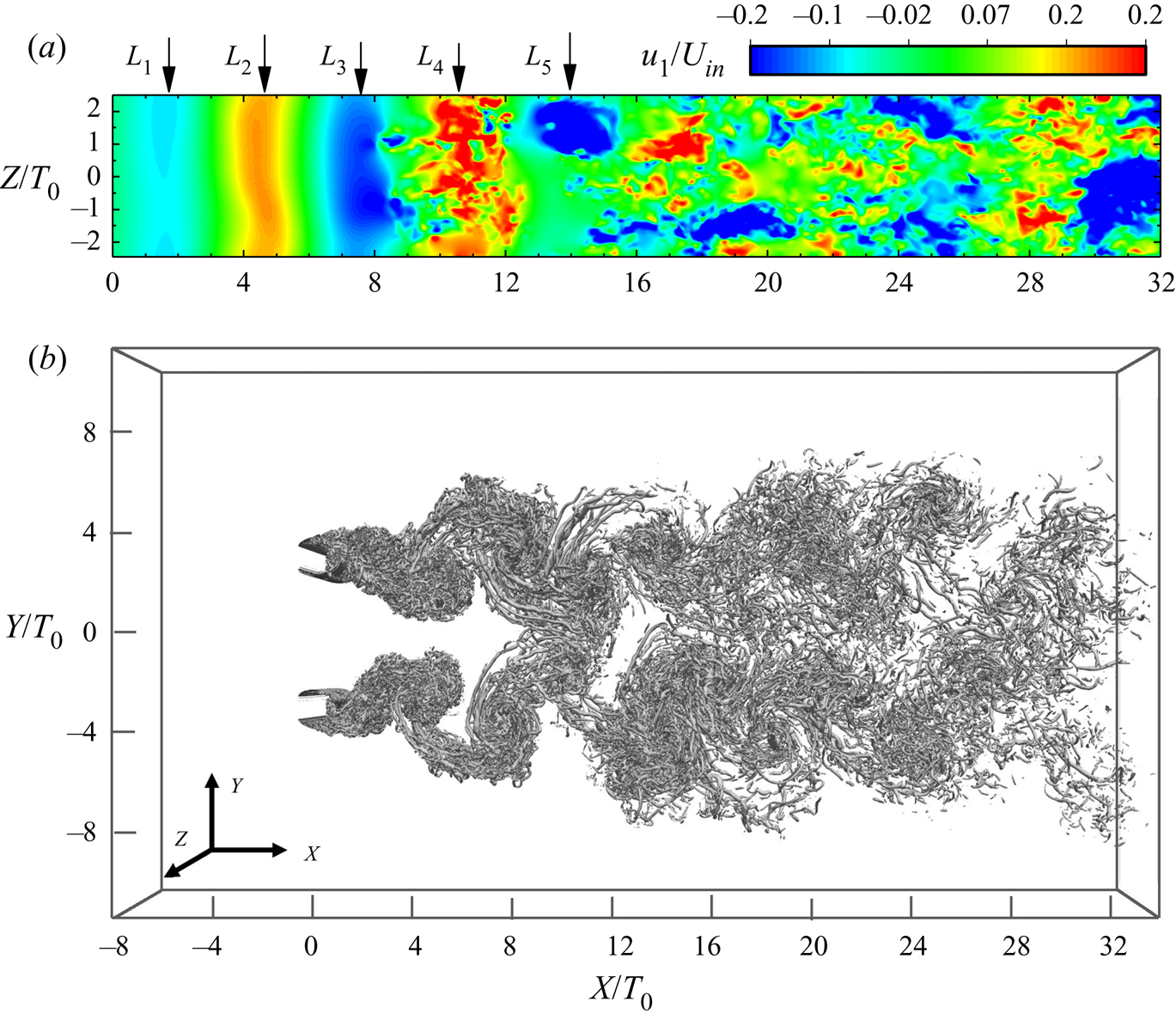
It is well known that behind a bluff body at a sufficiently large Reynolds number, large-scale spanwise structures can be formed, which may contribute to transport the turbulent kinetic energy. One may argue that even in a dual-wake flow there may also exist streamwise rib-like vortices between spanwise rolls. Figure 4(a) shows that periodical spanwise positive and negative strips can be found in the upstream region, which suggests the imprint of the large-scale coherent structures. The acceleration of the gap flow between two counter-rotating vortices (at  $L_1$ and
 $L_3$ locations) has already been reported (see figure 2(b) in Alam & Zhou (Reference Alam and Zhou2013)). One may easily verify that the periodical alternations of the positive and negative strips (negative strip at
 $L_1$,
 $L_3$ and
 $L_5$; positive strip at
 $L_2$ and
 $L_4$) are in accord with the vortex shedding behaviour, the Strouhal number of which is
 $St \simeq 0.142$. The isosurfaces of the normalized second invariant of the velocity gradient tensor
 $Q/(U_{in}/T_0)^2 = 5$ at the same time step are shown in figure 4(b), where
 $Q=- (A_{i j} A_{j i}/2)$ with
 $A_{i j}=\partial (u_{i} + U_{i}) / \partial x_{j}$ being the instantaneous velocity gradient tensor. Figure 4(b) confirms the very existence of the streamwise rib-like vortices. In the upstream region, the instantaneous velocity field along the spanwise direction is quasi-homogeneous, which allows us to make use of a spatial decomposition as will be discussed below. Also figure 4(b) shows that at the time step considered, antiphase vortex shedding (varicose mode) from the two cylinders can be observed. We also confirm that inphase vortex shedding behaviour (sinuous mode) can also be found behind the two cylinders (for economy of space not shown herein). However, the detailed characteristics of the vortex shedding behaviour (e.g. excitation and perishing of the antiphase/inphase vortex shedding, and switching between two modes) remain unclear, which is indeed an important topic but beyond the scope of the current study.
 $(a)$ Contour plot of the fluctuating streamwise velocity components
 $u_1/U_{in}$ in the
 $(X, Z)$ plane at
 $Y=0$ and
 $(b)$ visualization of the isosurfaces corresponding to
 $Q/(U_{in}/T_0)^2 = 5$. The two plots are obtained by using DNS data of the same time step.

3.2. Intermittency
To further study the observation that the turbulent flow owing to wake interactions can be highly intermittent in the upstream region (see figure 3a, figure 3 in Alam & Zhou (Reference Alam and Zhou2013) and figure 9 in Laizet et al. (Reference Laizet, Nedić and Vassilicos2015)) and to quantitatively assess the alternation between laminar and turbulent motion along the centreline, the intermittency factor  $\gamma$ and the conditional statistics are computed.
The intermittency factor  $\gamma$ is the probability that fluid points are in the turbulent region. More specifically,
 $\gamma$ is defined by
 \begin{equation} \gamma \equiv \frac{\text{number of time steps in the turbulent region}}{\text{total number of time steps}}. \end{equation}
In this study, vorticity norm is adopted to locate the turbulent–non-turbulent interfaces, and the intermittency factor  $\gamma$ is directly determined from the instantaneous vorticity field. If an appropriate vorticity magnitude threshold
 $\varOmega _{tr}(x,t)$ (written for simplicity as
 $\varOmega _{tr}$) is exceeded, the fluid motions can be considered to be in the turbulent region, and the algorithm for obtaining it is quite similar to that proposed by Zhou & Vassilicos (Reference Zhou and Vassilicos2017). The threshold
 $\varOmega _{tr}$ therefore depends on the instantaneous maximum
 $\varOmega (x,t)_{max}$ (written for simplicity as
 $\varOmega _{max}$) in a given
 $Y\text {--}Z$ plane.
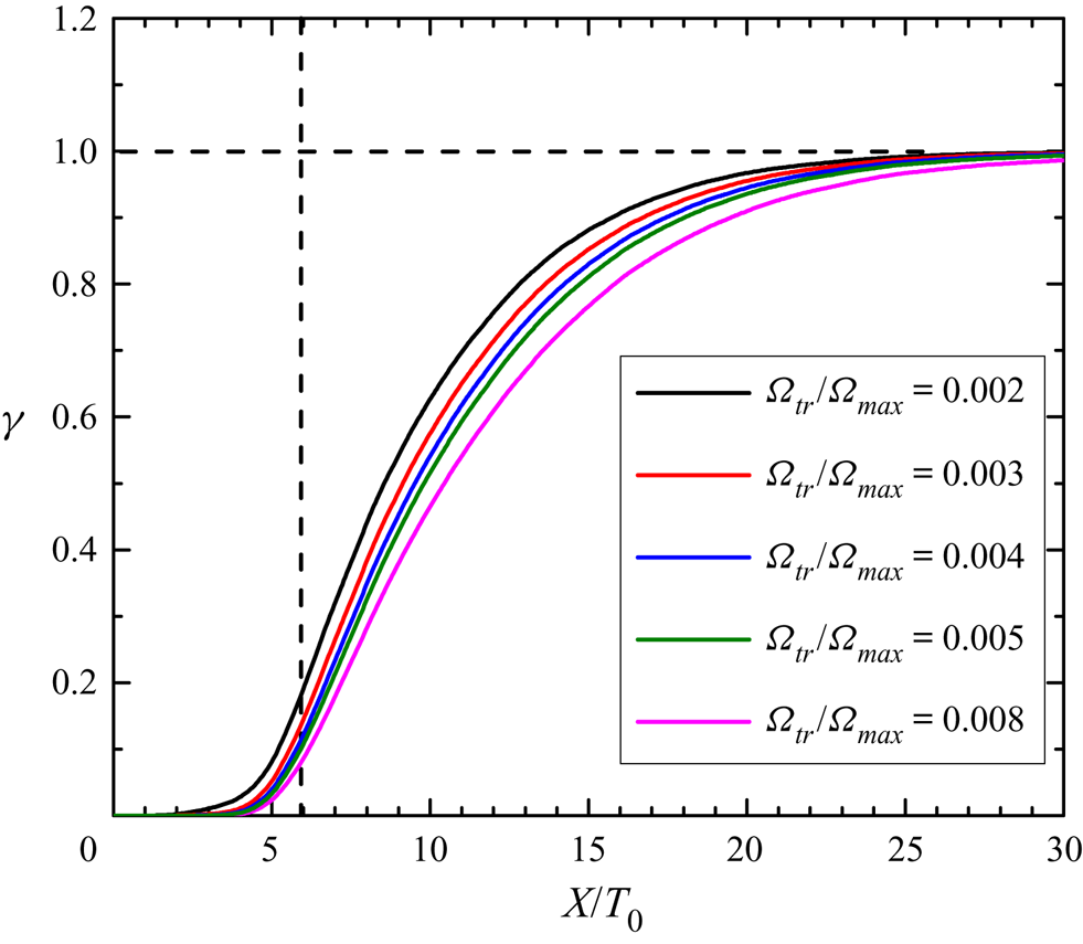
To investigate the evolution of the centreline intermittency  $\gamma$, the vorticity magnitude within the range
 $0.002 \le \varOmega _{tr}/ \varOmega _{max}\le 0.008$ is considered. It can be seen from figure 5 that in the range
 $0.003 \le \varOmega _{tr}/ \varOmega _{max}\le 0.005$, the profiles of
 $\gamma$ slightly depend on the threshold chosen. Therefore,
 $\varOmega _{tr}/ \varOmega _{max} = 0.004$ is chosen as the detection threshold. It should be stressed that this threshold level can be applied only to the centreline, rather than the two-dimensional
 $Y\text {--}Z$ plane.
Streamwise evolution of the intermittency factor  $\gamma$ along the centreline under different thresholds within the range
 $0.002 \le \varOmega _{tr}/\varOmega _{max}\le 0.008$. The dashed horizontal line denotes a fully turbulent state (i.e.
 $\gamma = 1$) and the vertical dashed line indicates
 $X/T_0=6$.

By and large, the turbulent flow along the centreline can be divided into three subregions (i.e. laminar/irrotational region, intermittent region and fully turbulent region), as can be seen from figure 5. The flow field is purely irrotational at  $X/T_0 \lesssim 4$. In the next extended region
 $4 \lesssim X/T_0 \lesssim 23$, where the flow is intermittent,
 $\gamma$ is slowly increasing. It should be noted that at the location
 $X/T_0=6$, the magnitude of the intermittency factor is quite small, i.e.
 $\gamma \simeq 0.14$, implying that the flow field is indeed highly intermittent, as suggested by figure 3. Only at the far downstream location, namely
 $X/T_0 \gtrsim 23$, does the flow field become almost fully turbulent (i.e.
 $\gamma \simeq 1$). The profile of
 $\gamma$ is quite different from that in a dual-jet flow, in which a rapid increase in
 $\gamma$ is observed (see figure 18b in Zhou et al. (Reference Zhou, Nagata, Sakai and Watanabe2018)).
3.3. Large-scale vortex shedding and turbulent motions
A step function  $\mathcal {H}(X,Y,Z,t)$ is used to characterize fluid motion at a given location
 $(X,Y,Z)$ at time
 $t$, namely
 $\mathcal {H} = 0$ if
 $\varOmega < \varOmega _{tr}$ (i.e. non-turbulent motion) and
 $\mathcal {H} = 1$ if
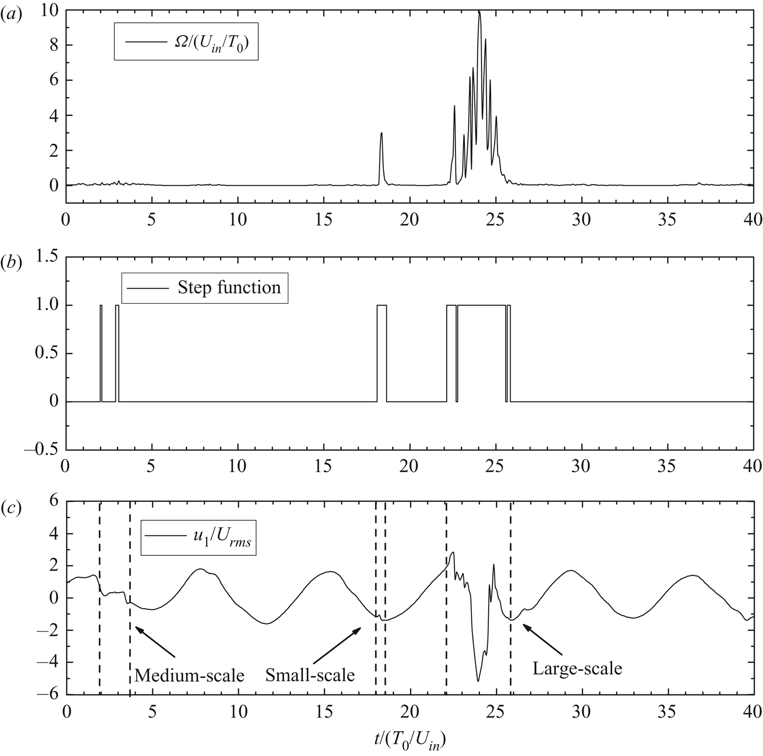
 $\varOmega \ge \varOmega _{tr}$ (i.e. turbulent motion). Figure 6(b) shows the time trace of the centreline step function
 $\mathcal {H}$ at
 $X/T_0 = 6$,
 $Y/T_0 = 0$ and an arbitrarily selected
 $Z$ location. The corresponding time evolutions of
 $\varOmega$ and the normalized fluctuating streamwise velocity
 $u_1/U_{rms}$ are shown in figures 6(a) and 6(c). By comparing figures 6(a), 6(b) and 6(c), it can be seen that most of the large-scale oscillation of
 $u_1$ is laminar. This observation is in accord with the small intermittency factor
 $\gamma \simeq 0.14$. Figure 6(c) shows a variety of velocity fluctuations, with extreme events occurring for large negative
 $u_1$. In the lee of the two solid bars, large-scale coherent structures with low speed are generated. One may expect that the transverse motions could occasionally convect the low-speed structures to the centreline, which leads to a negative skewness of the streamwise velocity fluctuations. See Zhou et al. (Reference Zhou, Nagata, Sakai and Watanabe2019) for a further explanation of the occurrence of extreme events. It was shown that the probability density function of the velocity fluctuations
 $u_1$ at
 $X/T_0=6$ exhibits significant fat tails, which are negatively skewed (see figure 8 in Zhou et al. (Reference Zhou, Nagata, Sakai and Watanabe2019)). There are approximately six cycles of large-scale periodic oscillations (i.e. vortex shedding) within the normalized time interval
 $t/( T_0/U_{in}) = 40$. One can roughly estimate the Strouhal number via
 $St \simeq 1/(40/6)=0.15$, which is indeed quite close to the exact Strouhal number, namely
 $St\simeq 0.142$.
Time evolution of  $(a)$ the magnitude of vorticity
 $\varOmega$,
 $(b)$ the step function
 $\mathcal {H}$ and
 $(c)$ the normalized fluctuating streamwise velocity component
 $u_1/U_{rms}$ at
 $X/T_0 = 6$ on the centreline.

Figure 6(c) shows that only one large-scale extreme event can be found within  $t/(T_0/U_{in})=40$. In our previous study (see figure 12b in Zhou et al. (Reference Zhou, Nagata, Sakai and Watanabe2019)), there are only two such large-scale extreme events (TF1 and TF2) within a time interval
 $t/(T_0/U_{in})=80$ and the periodic oscillation occurs approximately 11 times. Therefore, a rough estimation suggest that the time interval of the large-scale events is five times that of periodical oscillation. However, we have to emphasize that this evaluation approach can be somewhat inaccurate since there is no exact definition of what events are ‘large events’. It should be stressed that within large-scale fluctuations, small-scale fluctuations may also be observed. This phenomenological observation may suggest the existence of a continuous distribution of the one-dimensional energy spectrum of
 $u_1$. Moreover, a well-defined
 $-5/3$ energy spectrum can be found at
 $X/T_0 = 6$ (see figure 2a).
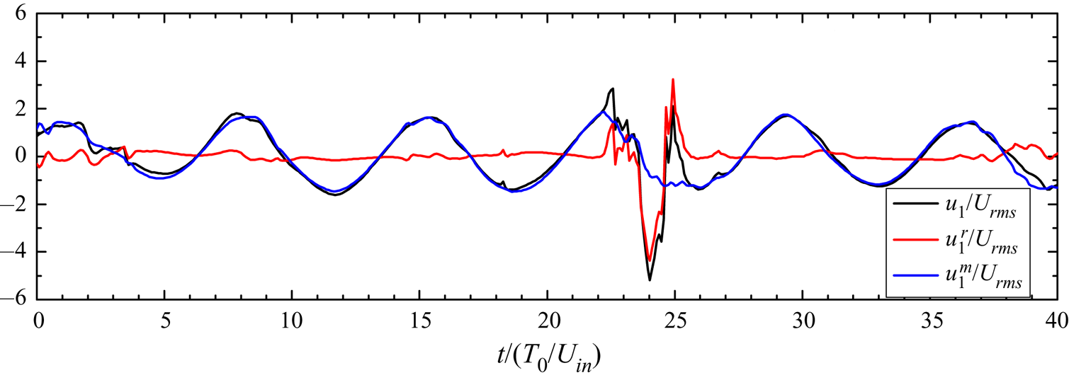
Figure 4(a) shows that for the fluctuating velocity field in the  $X\text {--}Z$ plane there are spanwise strips in the upstream region, which can be viewed as background movement. Therefore, the velocity fluctuations
 $u_1$ would be further decomposed into the spanwise average of instantaneous velocities
 $u_1^m$ and the residual part
 $u_1^r$, i.e.
 $u_1 = u_1^m + u_1^r$. Through this decomposition, one can evaluate the turbulent part without influence of background large-scale field. It can be seen from figure 7 that by removing the background velocity
 $u_1^m$ (periodical large-scale oscillation), except for the burst of extreme events, the magnitude of the remaining component
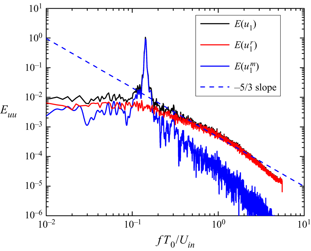
 $u_1^r$ can be negligibly small. Figure 8 indicates that the background part
 $u_1^m$ mainly contributes to the low-frequency range of the spectrum of
 $u_1$. In our previous study (Zhou et al. Reference Zhou, Nagata, Sakai and Watanabe2019), it was only suggested that ‘the approximate
 $-5/3$ power law in the high-frequency range is closely related to the occurrences of the extreme events’. Figures 7 and 8 clearly show that the residual part
 $u_1^r$ contains a wide range of scales, which can lead to a discernible power-law range with an exponent close to
 $-5/3$. The fluctuation of the residual part seems to be composed of the quiescent part and the intermittently passing eddy structure (
 $22 \lesssim t /(T_0 / U_{in}) \lesssim 26$).
Time evolution of  $u_1/U_{rms}$,
 $u_1^m/U_{rms}$ and
 $u_1^r/U_{rms}$ at
 $X/T_0 = 6$ on the centreline. The origin of time is the same as that in figure 6.

Energy spectra of the streamwise velocity fluctuation  $u_1$ and its two components (
 $u_1^m$ and
 $u_1^r$) at
 $X/T_0=6$.

The size (or the duration) of the intermittently passing eddy structure is approximately  $\Delta t /(T_{0}/U_{in}) \approx 4$ (
 $=26\text {--}22$). The inverse of this value roughly corresponds to the lower value of the ‘inertial subrange’ spectrum (
 $\,fT_0/U_{in} \simeq 0.25$) of the residual part.
A previous experimental study (Cuypers, Maurel & Petitheans Reference Cuypers, Maurel and Petitheans2003) revealed that vortex burst in a laminar flow is an elementary structure responsible for the celebrated  $-5/3$ spectra. It seems that even in a turbulent environment with wake interactions (i.e. in the near field of turbulent flows due to two parallel square cylinders Zhou et al. (Reference Zhou, Nagata, Sakai and Watanabe2019), a single square grid Paul et al. (Reference Paul, Papadakis and Vassilicos2017); Yasuda, Goto & Vassilicos (Reference Yasuda, Goto and Vassilicos2019), a regular grid Valente & Vassilicos (Reference Valente and Vassilicos2012); Isaza et al. (Reference Isaza, Salazar and Warhaft2014) and a fractal square grid Gomes-Fernandes et al. (Reference Gomes-Fernandes, Ganapathisubramani and Vassilicos2015); Laizet et al. (Reference Laizet, Nedić and Vassilicos2015)), the appearance of vortex burst structures may also lead to the celebrated
 $-5/3$ spectra. The intermittently passing isolated eddy structure (see figure 7) is a cause of the inertial subrange at
 $X/T_0=6$ for the dual-wake case.
It might be worth mentioning that the physical model proposed by Lundgren (Reference Lundgren1982) for intermittent fine structure to predict the origin of the  $-5/3$ spectra is directly derived from the vortex solutions of the Navier–Stokes equation, and the conventional dimensional analysis and the related hypothesis (local isotropy hypothesis and similarity hypotheses) are not involved. Therefore, in turbulent flow with vortex burst, the appearance of the
 $-5/3$ power law in spectral space does not suggest a 2/3 power law in real space. Only in Kolmogorov's flow (homogeneous and isotropic) with sufficiently high Reynolds number is the spectral equivalent of the
 $2/3$ power law the
 $-5/3$ scaling law, as hinted at by the Kolmogorov dimensional analysis.
4. One-point turbulent kinetic energy balance
As can be seen from figure 6, a wide range of excited scales can be found at  $X/T_0=6$, where the flow is highly intermittent. The existence of multiple length scales is owing to the nonlinear nature of the Navier–Stokes equation. Before delving into the scale-by-scale energy cascade, we first investigate the centreline evolution of the one-point turbulent kinetic energy budget, which, as shown in the following section, is actually closely related to the two-point energy budget.
4.1. Streamwise evolution of the one-point turbulent kinetic energy budget
The transport equation for the one-point turbulent energy budget reads
 \begin{align} \frac{\partial}{\partial t} \langle k \rangle &+ U_{j} \frac{\partial}{\partial x_{j}}\left(\frac{1}{2} {\langle u_{i} u_{i}\rangle}\right) = -\frac{\partial}{\partial x_{j}}\left(\langle u_{j} p\rangle\right) -\frac{\partial}{\partial x_{j}}\left(\frac{1}{2}\langle u_{i} u_{i} u_{j}\rangle\right)\nonumber\\ &\quad+\frac{\partial}{\partial x_{j}} (2 \nu \langle u_{i} s_{i j}\rangle) -\langle u_{i} u_{j} \rangle S_{i j}-2 \nu \langle s_{i j} s_{i j}\rangle, \end{align}
where
 \begin{equation} k= \frac{1}{2}( u_{i} u_{i}),\quad s_{i j}=\frac{1}{2}\left(\frac{\partial u_{i}}{\partial x_{j}}+\frac{\partial u_{j}}{\partial x_{i}}\right)\quad \textrm{and}\quad S_{i j}=\frac{1}{2}\left(\frac{\partial U_{i}}{\partial x_{j}}+\frac{\partial U_{j}}{\partial x_{i}}\right) \end{equation}
denote the fluctuating and mean strain rates, respectively. The operator  $\langle \ \rangle$ indicates an average over time and the homogeneous
 $Z$ direction. The terms in (4.1) can also be expressed in the form of
 \begin{equation} \left\langle \mathcal{A}_t^k \right\rangle + \left\langle \mathcal{A}^k \right\rangle = \left\langle \mathcal{T}_p^k \right\rangle + \left\langle \mathcal{T}_u^k \right\rangle + \left\langle \mathcal{T}_D^k \right\rangle + \left\langle \mathcal{P}^k \right\rangle - \left\langle \varepsilon^k\right\rangle. \end{equation}
It might be worth mentioning that the terms involved in the one-point turbulent energy budget are represented by the superscript  $k$. One can expect that the average unsteady term
 $\langle \mathcal {A}_t^k \rangle$ vanishes if the statistical convergence of terms in the turbulent kinetic energy equation is secured. Brief physical interpretations of the other terms in (4.3) are as follows. The advection term
 $\langle \mathcal {A}^k \rangle$ stands for the advection of the turbulent kinetic energy
 $\langle k \rangle$ by the mean flow. Since
 $U_2 = 0$ and
 $U_3 = 0$ along the centreline, evidently it can be seen that the advection term becomes
 $\langle \mathcal {A}^k \rangle \simeq U_{1} ({\partial }/{\partial x_{1}})\langle k\rangle$. The terms
 $\langle \mathcal {T}_p^k \rangle$,
 $\langle \mathcal {T}_u^k \rangle$ and
 $\langle \mathcal {T}_D^k \rangle$ represent transport of turbulent kinetic energy (i.e. spatial redistribution of energy) by pressure, turbulent fluctuation (or triple correlation) and viscous diffusion. The production term
 $\langle \mathcal {P}^k \rangle$, which is usually positive, indicates a connection between the fluctuating and the mean velocity fields, that is the kinetic energy is transferred from the mean field to the fluctuating field through the gradients of the mean velocities. The last term
 $\langle \varepsilon ^k \rangle$ is the dissipation term, through which the turbulent kinetic energy is converted into heat and obviously
 $\langle \varepsilon ^k \rangle$ is always positive.
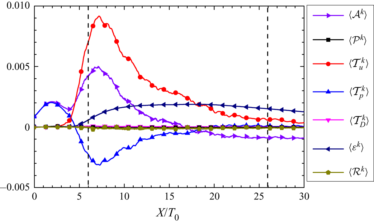
Figure 9 shows the streamwise evolution of the turbulent kinetic energy budget along the centreline, which clearly demonstrates that the one-point energy transfer can be considerably different with streamwise distance from the two square cylinders. In the laminar/irrotational region ( $X/T_0 \lesssim 4$), where the two wakes do not reach the centreline, (4.3) can be simplified as
 $\langle \mathcal {A}^k \rangle \simeq \langle \mathcal {T}_p^k \rangle$. This finding suggests that the increase of the turbulent kinetic energy is solely related to the non-local effects of the pressure force, which serves as a source term. On the other hand, the other terms in (4.3) (i.e
 $\langle \mathcal {T}_u^k \rangle$,
 $\langle \mathcal {T}_D^k \rangle$,
 $\langle \mathcal {P}^k \rangle$ and
 $\langle \varepsilon ^k \rangle$) are negligibly small.
Streamwise evolution of turbulent kinetic energy budget along the centreline. The two vertical dashed lines indicate  $X/T_0=6$ and 26 (the corresponding intermittency factors
 $\gamma$ are 0.14 and 1). The term
 $\langle \mathcal {R}^k\rangle$ stands for the residual balance, which would arise due to a lack of statistical convergence or numerical errors stemming from the DNS approach itself and the subsequent data processing.

In the highly intermittent region (e.g.  $X/T_0=6$), we are now left with
 $\langle \mathcal {A}^k \rangle \simeq \langle \mathcal {T}_p^k \rangle + \langle \mathcal {T}_u^k \rangle - \langle \varepsilon ^k \rangle$ and the pressure term
 $\langle \mathcal {T}_p^k \rangle$ serves as a sink term instead. It can be seen that the average magnitude of the dissipation term
 $\langle \varepsilon ^k \rangle$ is much smaller than
 $\langle \mathcal {A}^k \rangle$,
 $\langle \mathcal {T}_p^k \rangle$ and
 $\langle \mathcal {T}_u^k \rangle$. The small dissipation
 $\langle \varepsilon ^k \rangle$ is related to the fact that the flow is laminar for most of its time (i.e.
 $\gamma \simeq 0.14$ and also see figure 6) since the viscous dissipation in laminar flows with large-scale motion is considerably small. It has already been demonstrated by Paul et al. (Reference Paul, Papadakis and Vassilicos2017) that along the cylinder centreline even at a similar upstream location the dissipation term is a dominant term (see figure 7 in Paul et al. (Reference Paul, Papadakis and Vassilicos2017)). Obviously, this difference finds its root in the different turbulent state, that is, the corresponding wake flow in Paul et al. (Reference Paul, Papadakis and Vassilicos2017) is always turbulent (i.e.
 $\gamma \simeq 1$). The only source term is the turbulent transport term
 $\langle \mathcal {T}_u^k \rangle$, which is further explored below.
It is well known that the non-local pressure forces (drag force and lift force) are closely associated with the large-scale vortex shedding. In the lee of square bars, one would therefore reasonably argue that the influences of the larger-scale advection term and the non-local pressure term can be significant, as suggested by figure 9. The strength of the pressure term decreases with increasing downstream distance. And in the fully turbulent region, e.g.  $X/T_0=26$, the influence of the pressure term can be safely neglected. Consequently, the full one-point turbulent energy budget equation can further reduce to
 $\langle \mathcal {A}^k \rangle \simeq \langle \mathcal {T}_u^k \rangle - \langle \varepsilon ^k \rangle$. Also the dissipation term
 $\langle \varepsilon ^k \rangle$ becomes much larger than the turbulent transport term
 $\langle \mathcal {T}_u^k \rangle$ at
 $X/T_0=26$. This large dissipation term (i.e. loss of energy), which finds its root in the large intermittent factor
 $\gamma$, directly leads to a negative advection term and consequently a decrease in the turbulent kinetic energy. The continuous decreases in the two average transport terms, namely
 $\langle \mathcal {T}_p^k \rangle$ and
 $\langle \mathcal {T}_u^k \rangle$, at
 $X/T_0 \ge 7$ also reflect the fact that the degree of homogeneity of the turbulent flow is improved around the centreline with downstream distance.
To further investigate the redistribution of the turbulent kinetic energy, we decompose the two non-negligible transport terms (i.e.  $\langle \mathcal {T}_p^k \rangle$ and
 $\langle \mathcal {T}_u^k \rangle$) into three components:
 \begin{align} \left\langle \mathcal{T}_u^k \right\rangle &=\left\langle \mathcal{T}_{u,x}^k \right\rangle + \left\langle \mathcal{T}_{u,y}^k \right\rangle + \left\langle \mathcal{T}_{u,z}^k \right\rangle \nonumber\\ &=-\frac{\partial}{\partial x_{1}}\left(\frac{1}{2}{\left\langle u_{i} u_{i}u_{1}\right\rangle}\right) -\frac{\partial}{\partial x_{2}}\left(\frac{1}{2}{\left\langle u_{i} u_{i}u_{2}\right\rangle}\right) -\frac{\partial}{\partial x_{3}}\left(\frac{1}{2}{\left\langle u_{i} u_{i}u_{3}\right\rangle}\right) \end{align}
and
 \begin{align} \left\langle \mathcal{T}_p^k \right\rangle & = \left\langle \mathcal{T}_{p,x}^k \right\rangle + \left\langle \mathcal{T}_{p,y}^k \right\rangle+\left\langle\mathcal{T}_{p,z}^k \right\rangle\nonumber\\ & =-\frac{\partial}{\partial x_{1}}\left\langle u_{1} p\right\rangle -\frac{\partial}{\partial x_{2}}\left\langle u_{2} p\right\rangle -\frac{\partial}{\partial x_{3}}\left\langle u_{3} p\right\rangle. \end{align}
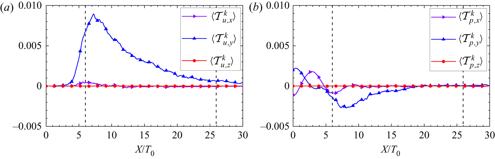
Figure 10 clearly demonstrates that the transport of the kinetic energy mainly occurs in the vertical direction, that is  $\langle \mathcal {T}_u^k \rangle \simeq \langle \mathcal {T}_{u,y}^k \rangle$ and
 $\langle \mathcal {T}_p^k \rangle \simeq \langle \mathcal {T}_{p,y}^k \rangle$. At the highly intermittent location (
 $X/T_0=6$), the turbulent transport term, the dominant source term, which is directly related to the growth and interactions of the two wakes, transports the turbulent kinetic energy towards the centreline. The vertical pressure term
 $\langle \mathcal {T}_{p,y}^k \rangle$, in contrast, acts like a sink and transports the kinetic energy away from the centreline. In other words, part of
 $\langle \mathcal {T}_u^k \rangle$ is then transferred back to the two turbulent wakes through the non-local pressure force.
Streamwise evolution of  $(a)$ three components of the turbulent transport term
 $\langle \mathcal {T}_{u}^k \rangle$ (i.e.
 $\langle \mathcal {T}_{u,x}^k \rangle$,
 $\langle \mathcal {T}_{u,y}^k \rangle$ and
 $\langle \mathcal {T}_{u,z}^k \rangle$) and
 $(b)$ three components of the pressure transport term
 $\langle \mathcal {T}_{p}^k \rangle$ (i.e.
 $\langle \mathcal {T}_{p,x}^k \rangle$,
 $\langle \mathcal {T}_{p,y}^k \rangle$ and
 $\langle \mathcal {T}_{p,z}^k \rangle$) along the centreline.

4.2. Sweeping and non-local effects
The flow field at  $X/T_0=6$ is characterized by energetic large-scale vortex shedding, which leads to direct interaction/coupling between large-scale motions and small-scale motions. Moreover, the flow is highly intermittent, i.e.
 $\gamma =0.14$. The existence of pairs of counter-rotating vortices (see figure 4) can result in a quasi-sweeping mechanism, through which small-scale turbulent motions can be transported by periodical large-scale vortex shedding motions. The sweeping decorrelation hypothesis, which actually originates from the Taylor frozen hypothesis, assumes that the Lagrangian acceleration of a fluid particle is considerably small, that is,
 $\textrm {D}\boldsymbol {u}/\textrm {D} t = {\partial \boldsymbol {u} }/{\partial t} + \boldsymbol {u}\boldsymbol {\cdot } \boldsymbol {\nabla } \boldsymbol {u} \simeq 0.$ If the sweeping decorrelation hypothesis holds, the one-point kinetic energy budget (i.e. (4.3)) can simplify to
 $\langle \mathcal {A}^k \rangle \simeq \langle \mathcal {T}_u^k \rangle$ since
 $\langle \mathcal {P}^k \rangle \simeq 0$ and the corresponding second-order structure function vanishes. It might be worth noting that the sweeping decorrelation hypothesis does not necessarily suggest that the Lagrangian acceleration is always zero, as has already been stressed by Tsinober (Reference Tsinober2009). More precisely, the local acceleration and the convective acceleration tend to cancel out each other so that
 $|{\textrm {D} \boldsymbol {u} }/{\textrm {D} t}| \ll |{\partial \boldsymbol {u} }/{\partial t}|$ and
 $|{\textrm {D} \boldsymbol {u} }/{\textrm {D} t}| \ll |\boldsymbol {u}\boldsymbol {\cdot } \boldsymbol {\nabla } \boldsymbol {u}|$.
To quantitatively evaluate the strength of the statistical correlation between the two quantities  $\mathcal {A}^k$ and
 $\mathcal {T}_u^k$ along the centreline, we resort to the so-called correlation coefficients:
 \begin{equation} \rho(\mathcal{A}^k,\mathcal{T}_u^k)=\langle (\mathcal{A}^k(x,t)- \langle \mathcal{A}^k(x,t) \rangle)(\mathcal{T}_u^k(x,t) - \langle \mathcal{T}_u^k(x,t) \rangle) \rangle/(\sigma_{\mathcal{A}^k} \sigma_{\mathcal{T}_u^k}), \end{equation}
where  $\sigma$ represents the standard deviation of a time-dependent variable. One may expect a discernible positive correlation between
 $\mathcal {A}^k$ and
 $\mathcal {T}_u^k$.
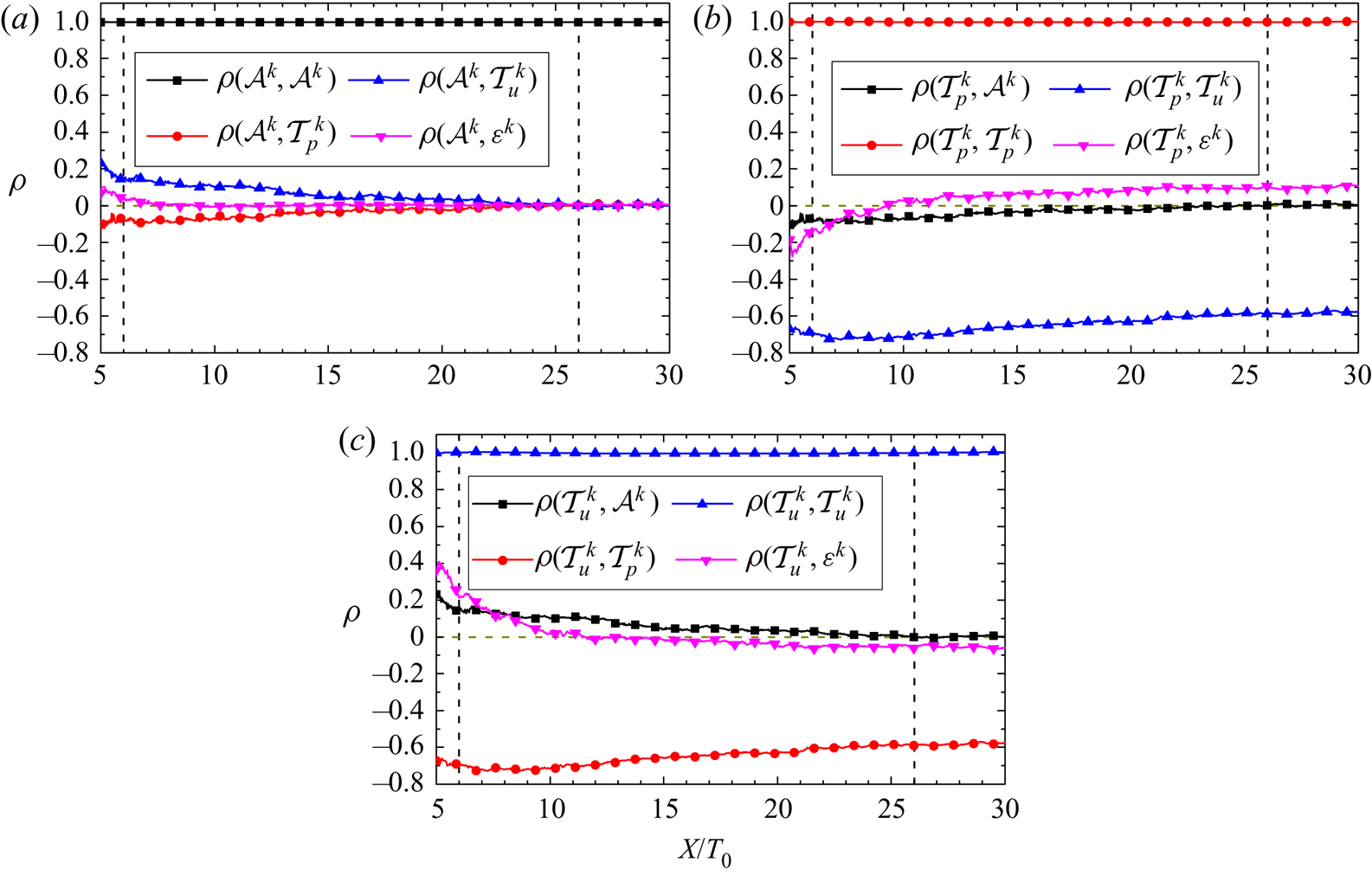
Figure 11(a) shows that a discernible correlation can indeed be found in the upstream region, that is at  $X/T_0 =6$,
 $\rho (\mathcal {A}^k, \mathcal {T}_u^k) \simeq 0.15$. With increasing streamwise distance, the sweeping effects continuously decrease. Consequently,
 $\rho (\mathcal {A}^k, \mathcal {T}_u^k) \simeq 0$ at
 $X/T_0 =26$. Similarly, we also calculate other correlation coefficients between the four significant terms (
 $\mathcal {A}^k$,
 $\mathcal {T}_p^k$,
 $\mathcal {T}_u^k$ and
 $\varepsilon ^k$) in (4.3) to reveal their intrinsic correlations. As can be seen from figure 11, the most pronounced correlation is the one between the two transport terms (i.e.
 $\mathcal {T}_p^k$ and
 $\mathcal {T}_u^k$), whose value lies between
 $-0.8$ and
 $-0.6$. And the lasting significant negative correlation coefficient
 $\rho (\mathcal {T}_p^k, \mathcal {T}_u^k)$ is obviously related to the non-locality of incompressible turbulent flows (i.e.
 $\boldsymbol {\nabla } \boldsymbol {\cdot }(\boldsymbol {u} \boldsymbol {\cdot } \boldsymbol {\nabla } \boldsymbol {u})=-\nabla ^{2} P$). The significant negative correlation
 $\rho (\mathcal {T}_p^k, \mathcal {T}_u^k)$ also to some extent reflects Bernoulli's principle, although Bernoulli's principle is applied only to isentropic flow. It might be worth mentioning that Lumley (Reference Lumley1978) has already proposed the model
 $\langle u_ip \rangle = -\langle u_iu_ju_j \rangle /5$ for the pressure transport in nearly homogeneous turbulence. Therefore, the significant negative correlation between turbulent transport
 $\mathcal {T}_u^k$ and pressure transport
 $\mathcal {T}_p^k$ terms is perhaps not surprising. This finding further implies that there is strong statistical cancellation between the pressure transport term
 $\langle \mathcal {T}_p^k \rangle$ and the turbulent transport term
 $\langle \mathcal {T}_u^k \rangle$. The small but discernible correlation coefficients
 $\rho (\varepsilon ^k, \mathcal {T}_u^k)$ and
 $\rho (\varepsilon ^k, \mathcal {T}_p^k)$ in the downstream region suggest that there is a weak link between the small-scale variables (i.e.
 $\varepsilon ^k$ and
 $\mathcal {T}_u^k$;
 $\varepsilon ^k$ and
 $\mathcal {T}_p^k$), which is certainly a topic for future work.
Streamwise evolution of the correlation coefficients along the centreline.  $(a)$ Correlation coefficients between
 $\mathcal {A}^k$ and
 $\mathcal {A}^k$,
 $\mathcal {T}_p^k$,
 $\mathcal {T}_u^k$ and
 $\varepsilon ^k$;
 $(b)$ correlation coefficients between
 $\mathcal {T}_p^k$ and
 $\mathcal {A}^k$,
 $\mathcal {T}_p^k$,
 $\mathcal {T}_u^k$ and
 $\varepsilon ^k$;
 $(c)$ correlation coefficients between
 $\mathcal {T}_u^k$ and
 $\mathcal {A}^k$,
 $\mathcal {T}_p^k$,
 $\mathcal {T}_u^k$ and
 $\varepsilon ^k$. The two vertical dashed lines indicate
 $X/T_0=6$ and 26, respectively.

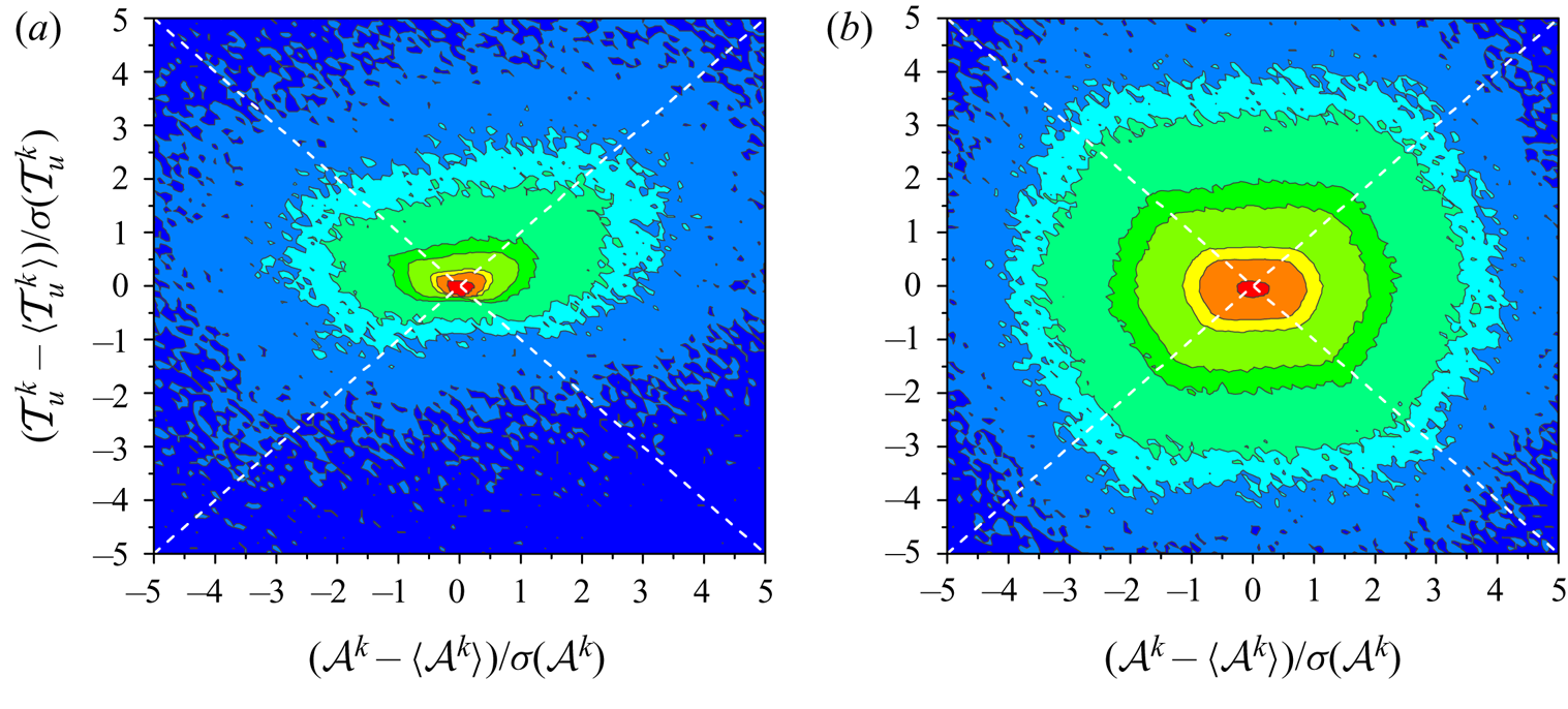
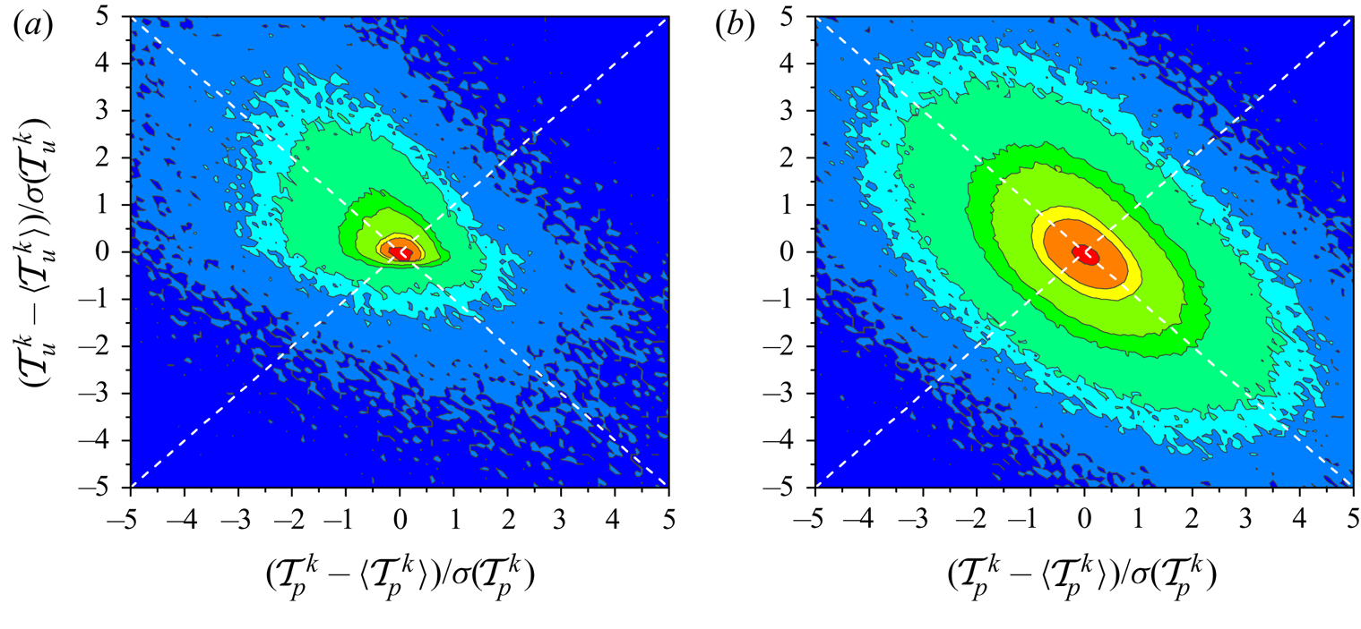
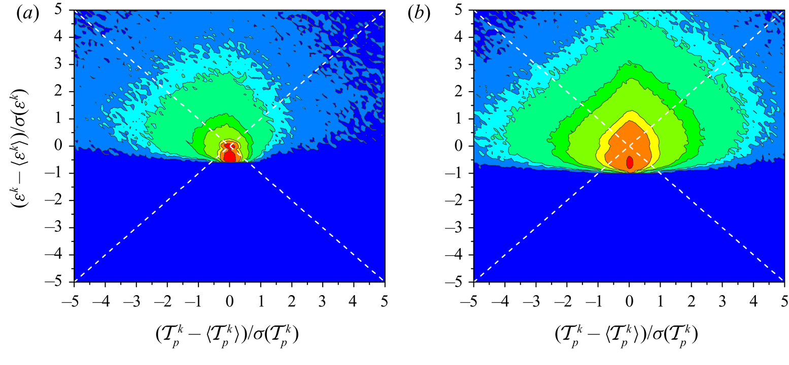
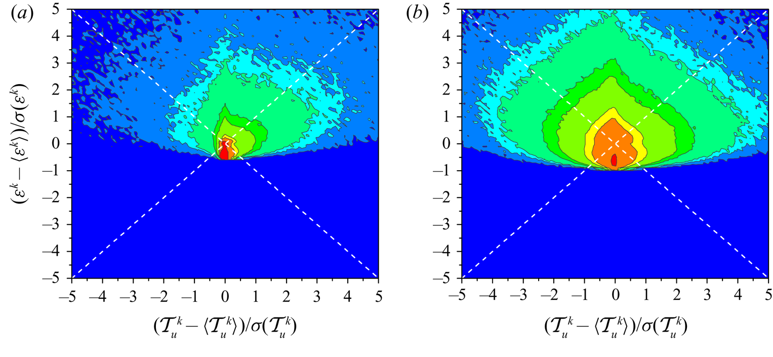
The joint probability distribution functions (PDFs) of  $(\mathcal {A}^k -\langle \mathcal {A}^k \rangle , \mathcal {T}_u^k - \langle \mathcal {T}_u^k \rangle )$,
 $(\mathcal {T}_p^k -\langle \mathcal {T}_p^k \rangle , \mathcal {T}_u^k -\langle \mathcal {T}_u^k \rangle )$,
 $(\mathcal {T}_p^k -\langle \mathcal {T}_p^k \rangle , \varepsilon ^k- \langle \varepsilon ^k \rangle )$ and
 $(\mathcal {T}_u^k -\langle \mathcal {T}_u^k \rangle , \varepsilon ^k- \langle \varepsilon ^k \rangle )$ at
 $X/T_0=6$ and
 $26$ are plotted in figures 12–15. Generally speaking, the contour lines of the joint PDFs at
 $X/T_0=6$ are less symmetric than those at the downstream location
 $X/T_0=26$. For instance, the contour lines of
 $\mathcal {T}_u^k$ at
 $X/T_0=6$ are positively skewed with respect to the horizontal line instead of being symmetric, suggesting that their fluctuating components tend to have intense positive values. The unsymmetric contour lines are related to the uneven probability distribution of the streamwise fluctuations (see figures 8 and 10 in Zhou et al. (Reference Zhou, Nagata, Sakai and Watanabe2019)).
Joint PDFs of  $\mathcal {A}^k- \langle \mathcal {A}^k \rangle$ and
 $\mathcal {T}_u^k - \langle \mathcal {T}_u^k \rangle$ at
 $(a)$
 $X/T_0=6$ and
 $(b)$
 $X/T_0=26$. The eight contour levels plotted are 1, 0.1, 0.05, 0.01, 0.005, 0.001, 0.0005 and 0.0001, respectively.

Joint PDFs of  $\mathcal {T}_p^k - \langle \mathcal {T}_p^k \rangle$ and
 $\mathcal {T}_u^k - \langle \mathcal {T}_u^k \rangle$ at
 $(a)$
 $X/T_0=6$ and
 $(b)$
 $X/T_0=26$. The eight contour levels plotted are 1, 0.1, 0.05, 0.01, 0.005, 0.001, 0.0005 and 0.0001, respectively.

Joint PDFs of  $\mathcal {T}_p^k - \langle \mathcal {T}_p^k \rangle$ and
 $\varepsilon ^k- \langle \varepsilon ^k \rangle$ at
 $(a)$
 $X/T_0=6$ and
 $(b)$
 $X/T_0=26$. The eight contour levels plotted are 1, 0.1, 0.05, 0.01, 0.005, 0.001, 0.0005 and 0.0001, respectively.

Joint PDFs of  $\mathcal {T}_u^k - \langle \mathcal {T}_u^k \rangle$ and
 $\varepsilon ^k- \langle \varepsilon ^k \rangle$ at
 $(a)$
 $X/T_0=6$ and
 $(b)$
 $X/T_0=26$. The eight contour levels plotted are 1, 0.1, 0.05, 0.01, 0.005, 0.001, 0.0005 and 0.0001, respectively.

Before closing this section, we summarize the characteristics of the one-point turbulent kinetic energy budget at the two selected locations (i.e.  $X/T_0=6 \text { and } 26$). In the upstream region, where the flow is highly intermittent and also highly inhomogeneous, the two transport terms (i.e.
 $\langle \mathcal {T}_u^k \rangle$ and
 $\langle \mathcal {T}_p^k \rangle$) play significant roles in the energy budget and the dissipation term is considerably small. However, as the homogeneity and the intermittency factor increase with downstream distance, the strength of the two transport terms continuously decreases and the dissipation term becomes the dominant term at
 $X/T_0=26$.
5. The KHMH equation and scale-by-scale energy cascade
In the preceding section, the one-point turbulent kinetic energy budget is investigated, which demonstrates that the energy transfer mechanism at  $X/T_0 =6$ is quite different from that at
 $X/T_0=26$. Here, we proceed one step further to provide a more complete picture of energy transfer by investigating the corresponding two-point energy budgets, which could provide some insight into the nature of the non-Kolmogorov
 $-5/3$ spectra at
 $X/T_0=6$, where
 $\gamma \simeq 0.14$. Note that in previous relevant studies, only the two-point energy transfer in fully turbulent flows (i.e. grid-generated turbulence (Gomes-Fernandes et al. Reference Gomes-Fernandes, Ganapathisubramani and Vassilicos2015; Valente & Vassilicos Reference Valente and Vassilicos2015), turbulent wake (Portela et al. Reference Portela, Papadakis and Vassilicos2017), homogeneous isotropic turbulence (Goto & Vassilicos Reference Goto and Vassilicos2016; Yasuda & Vassilicos Reference Yasuda and Vassilicos2018)) has been considered. The two-point energy transfer behaviour in highly intermittent flow fields, which is an important part of this study, however, still remains unclear. Moreover, the two-point energy cascade processes at the fully turbulent location
 $X/T_0=26$ are also explored for comparison.
5.1. The KHMH equation
The average generalized Kármán–Howarth equation reads
 \begin{align} &\frac{\partial \langle \delta q^2 \rangle}{\partial t} + \frac{\partial \dfrac{U_i^++U_i^-}{2} \langle \delta q^2 \rangle}{\partial x_i} + \frac{\partial \langle \delta u_i \delta q^2 \rangle}{\partial r_i} + \frac{\partial \delta U_i \langle \delta q^2 \rangle}{\partial r_i} \nonumber\\ &\quad = - 2 \langle \delta u_i \delta u_j \rangle \frac{\partial \delta U_j}{\partial r_i} - \langle (u_i^+ + u_i^-)\delta u_j \rangle \frac{\partial\delta U_j}{\partial x_i} -\frac{\partial \left\langle \dfrac{u_i^+ + u_i^-}{2}\delta q^2 \right\rangle}{\partial x_i} -2\frac{\partial \langle \delta u_i \delta p \rangle}{\partial x_i} \nonumber\\ &\qquad +\frac{1}{2} \nu \frac{\partial^2 \langle \delta q^2 \rangle}{\partial x_i\partial x_i} +2 \nu \frac{\partial^2 \langle \delta q^2 \rangle}{\partial r_i\partial r_i} -4 \nu \left(\left\langle \frac{\partial \delta u_j }{\partial x_i} \frac{\partial \delta u_j }{\partial x_i} \right\rangle + \frac{1}{4} \left\langle \frac{\partial \delta u_j }{\partial r_i} \frac{\partial \delta u_j }{\partial r_i} \right\rangle\right), \end{align}
where  $x_i=(X_i^+ + X_i^-)/2$,
 $r_i= X_i^+ - X_i^-$,
 $\delta q^2 = (\delta u_i)^2 = (u_i^+ -u_i^-)^2$ with summation over index
 $i = 1, 2, 3$. Following Gomes-Fernandes et al. (Reference Gomes-Fernandes, Ganapathisubramani and Vassilicos2015) the terms in (5.1) can also be expressed in the form of
 \begin{equation} \langle \mathcal{A}_t \rangle + \langle \mathcal{A} \rangle + \langle \varPi \rangle + \langle \varPi_U \rangle = \langle \mathcal{P} \rangle + \langle \mathcal{T}_u \rangle + \langle \mathcal{T}_p \rangle + \langle \mathcal{D}_x \rangle + \langle \mathcal{D}_r \rangle - \langle \varepsilon_r \rangle. \end{equation}
A detailed physical interpretation of each term in (5.2) has already be given in previous studies (e.g. Marati et al. Reference Marati, Casciola and Piva2004; Portela et al. Reference Portela, Papadakis and Vassilicos2017; Valente & Vassilicos Reference Valente and Vassilicos2015; Gomes-Fernandes et al. Reference Gomes-Fernandes, Ganapathisubramani and Vassilicos2015).
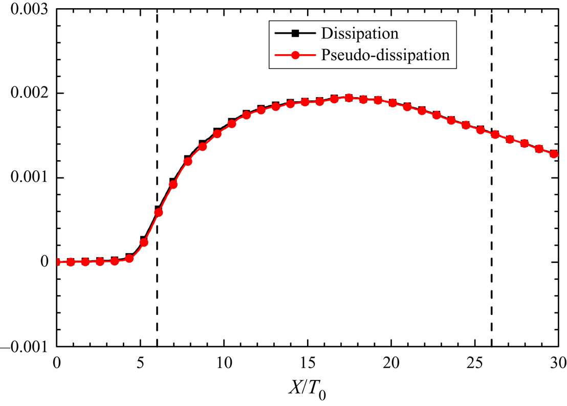
It is worth recalling that the viscous dissipation term  $\langle \varepsilon _r \rangle$ can also be rewritten as
 \begin{equation} \langle \varepsilon_r \rangle=\frac{1}{2} \nu \left\langle \frac{\partial u_j^+ }{\partial X_i^+} \frac{\partial u_j^+ }{\partial X_i^+} + \frac{\partial u_j^- }{\partial X_i^-} \frac{\partial u_j^-}{\partial X_i^-} \right\rangle \end{equation}
and is the average of the pseudo-dissipation at  $X^+$ and
 $X^-$. Actually,
 $\langle \varepsilon _r \rangle$ is also referred to as the ‘dissipation’ term in the two-point energy balance, since the difference between the average true dissipation
 $\langle 2\nu s_{ij}s_{ij} \rangle$ in the one-point turbulent energy budget (i.e. in (4.1)) and the average pseudo-dissipation
 $\langle \varepsilon _r \rangle$ is quite small (Pope Reference Pope2000).
With sufficiently high Reynolds numbers, according to the Richardson–Kolmogorov equilibrium view of energy cascade in the ‘inertial range’, the full KHMH equation (5.2) can reduce to  $\langle \varPi \rangle \simeq - \langle \varepsilon _r \rangle$, which sets the basis for the
 $-5/3$ energy spectra or equivalently the
 $2/3$ scaling of the second-order structure function (e.g. Marati et al. Reference Marati, Casciola and Piva2004; Gomes-Fernandes et al. Reference Gomes-Fernandes, Ganapathisubramani and Vassilicos2015; Valente & Vassilicos Reference Valente and Vassilicos2015; Portela et al. Reference Portela, Papadakis and Vassilicos2017). The second important implication of the equilibrium energy cascade assumption is the Taylor dissipation law. However, recently it has been numerically demonstrated by Goto & Vassilicos (Reference Goto and Vassilicos2015, Reference Goto and Vassilicos2016) that such local equilibrium hypothesis is not valid even in homogeneous and isotropic turbulence. The absence of the equilibrium energy cascade stems from the finite time required for the energy at large scales to cascade down to the small/dissipative scales. In a recent numeral study of homogeneous isotropic turbulence by Yasuda & Vassilicos (Reference Yasuda and Vassilicos2018), it has been demonstrated that the zero-average unsteady terms (
 $\langle \mathcal {A}_t \rangle$,
 $\langle \mathcal {T}_u \rangle$ and
 $\langle \mathcal {T}_p \rangle$) also play indispensable roles in the process of energy cascade albeit these terms are absent in the average picture. The nonlinear energy transfer term
 $\varPi$ is the divergence of the interscale energy flux
 $\langle \delta \boldsymbol {u} \delta q^2 \rangle$ in
 $r$ space as can be easily proved by using Gauss's divergence theorem. It is believed that the interscale energy flux integrated over all directions in the intermittent range is always negative, indicating a forward cascade, that is, the kinetic energy on average cascades from large to small scales. The idea of forward energy cascade was firstly proposed in Richardson's celebrated poem (Richardson Reference Richardson1922). By decomposition of the velocity field into coherent and random parts, Thiesset et al. (Reference Thiesset, Danaila, Antonia and Zhou2011) investigated the scale-by-scale energy transfer associated with coherent motion in a cylinder wake flow by resorting to a simplified version of the KHMH equation.
To compute terms in (5.1), the correlations between the two points  $X^+$ and
 $X^-$ are used. For example, the turbulent transport term is computed by
 \begin{equation} \mathcal{T}_u = - \frac{1}{4} \left(u_j^+ + u_j^-\right) \left(u_i^+ - u_i^-\right)\left( \frac{\partial u_i^+ }{\partial X_j^+} - \frac{\partial u_i^- }{\partial X_j^-}\right). \end{equation}
The flow considered here is statistically steady and the unsteady term  $\langle \mathcal {A}_t \rangle$ would vanish if the number of time steps,
 $N_{total}$, is sufficient to achieve statistical convergence. For computation, the average KHMH equation consequently becomes
 \begin{equation} \langle \mathcal{A} \rangle + \langle \varPi \rangle + \langle \varPi_U \rangle = \langle \mathcal{P} \rangle + \langle \mathcal{T}_u \rangle + \langle \mathcal{T}_p \rangle + \langle \mathcal{D}_x \rangle + \langle \mathcal{D}_r \rangle - \langle \varepsilon_r \rangle + \langle \mathcal{R} \rangle, \end{equation}
where  $\langle \mathcal {R} \rangle$ is the residual balance, which would arise because of numerical errors associated with numerical simulation and the subsequent data processing. The implications of the residual balance term
 $\langle \mathcal {R} \rangle$ are twofold. First, the relativity small magnitude of the residual term
 $\langle \mathcal {R} \rangle$ implies that
 $\langle \mathcal {A} \rangle + \langle \varPi \rangle + \langle \varPi _U \rangle$ and
 $\langle \mathcal {P} \rangle + \langle \mathcal {T}_u \rangle + \langle \mathcal {T}_p \rangle + \langle \mathcal {D}_x \rangle + \langle \mathcal {D}_r \rangle - \langle \varepsilon _r \rangle$ are in good balance and validates the statistical convergence, namely
 $\langle \mathcal {A}_t \rangle \simeq 0$. Second, the small residual term
 $\langle \mathcal {R} \rangle$ lends further credence to our DNSs as well as the subsequent data processing. As is shown in the following section, the residual term
 $\langle \mathcal {R} \rangle$ is indeed negligibly small as it should be.
5.2. Scale-by-scale energy cascade at the two chosen locations
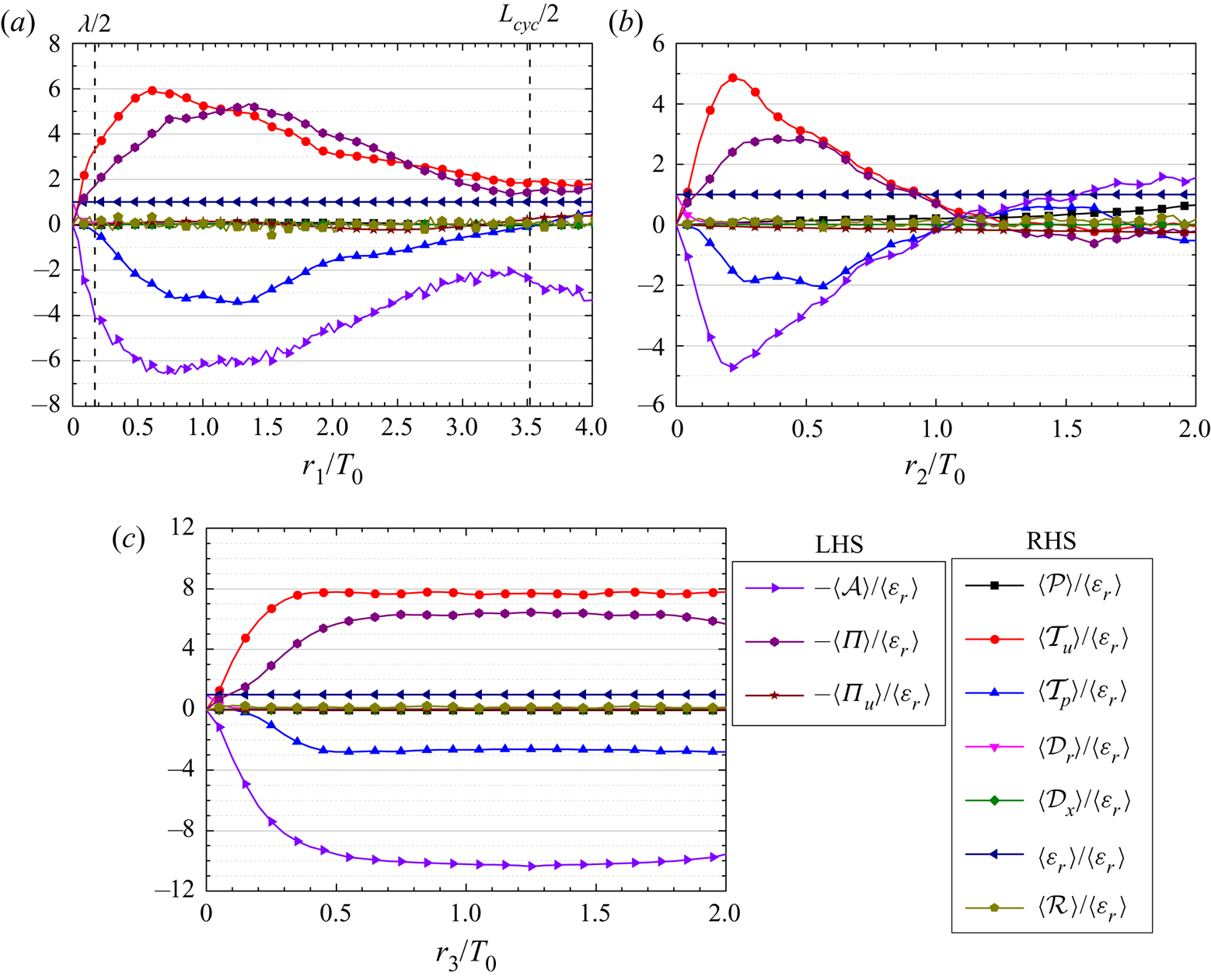
The average scale-by-scale energy transfer along  $r_1$,
 $r_2$ and
 $r_3$ at
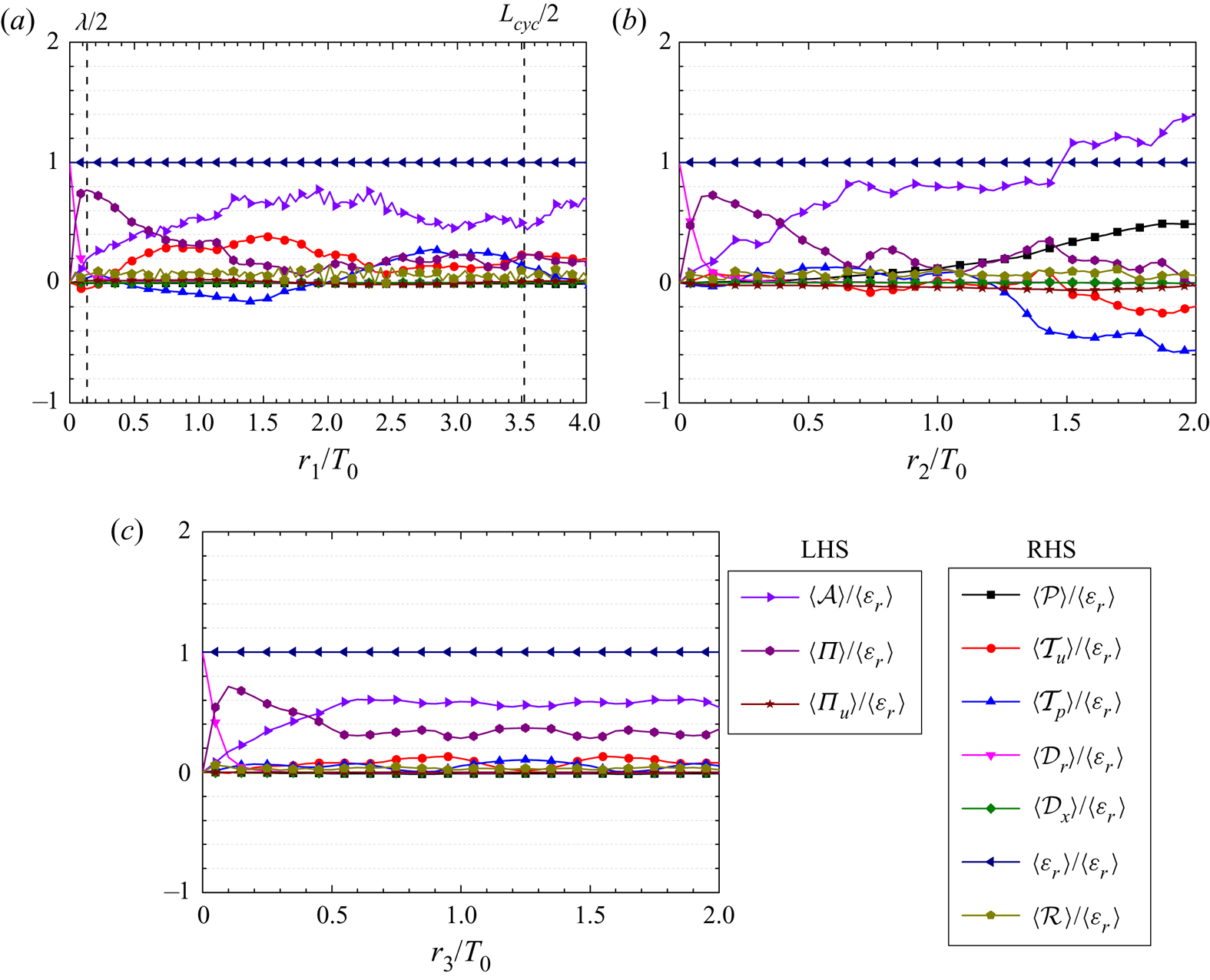
 $X/T_{0}=6$, where the energy spectrum exhibits a well-defined
 $-5/3$ power-law range for over one decade, is plotted in figure 16. Similar to what we did for the one-point turbulent kinetic energy balance, to evaluate the two-point scale-by-scale energy cascade, the full time series of the velocity signals are used and the statistical averages are taken over the statistically homogeneous direction
 $Z$. In this work, two-point energy transfer over long separation ranges is considered, which enables us to study the influence of the large-scale vortex shedding, which appears to define the beginning of the
 $-5/3$ power-law spectra, and the energy transfer from energetic dual wakes to the centre of the flow field. For a zero separation distance, it can be seen that the only two remaining terms are
 $\langle \mathcal {D}_r \rangle$ and
 $\langle \varepsilon _r \rangle$, that is,
 $\langle \mathcal {D}_r \rangle = \langle \varepsilon _r \rangle$, as it should be. It can be also seen that except at very small scales, which is comparable to
 $\lambda /2$, the linear energy transport term
 $\langle \varPi _U \rangle$, the production term
 $\langle \mathcal {P} \rangle$ and the viscous diffusion terms (both
 $\langle \mathcal {D}_x \rangle$ and
 $\langle \mathcal {D}_r \rangle$) can be safely neglected. For instance, within the intermediate separation range
 $\lambda /2 \lesssim r \lesssim L_{cyc}/2$, along
 $r_1$ the remaining terms in (5.2) are
 $\langle \mathcal {A} \rangle$,
 $\langle \varPi \rangle$,
 $\langle \mathcal {T}_u \rangle$,
 $\langle \mathcal {T}_p \rangle$ and
 $\langle \varepsilon _r \rangle$ and the KHMH equation can be approximated by
 \begin{equation} \langle \mathcal{A} \rangle + \langle \varPi \rangle \simeq \langle \mathcal{T}_u \rangle + \langle \mathcal{T}_p \rangle - \langle \varepsilon_r\rangle, \end{equation}
which is in direct contrast to the Richardson–Kolmogorov equilibrium view of energy cascade, namely  $\langle \varPi \rangle \simeq - \langle \varepsilon _r \rangle$. Here,
 $L_{cyc}$ is the size of the large-scale vortex shedding. In addition, the average magnitudes of
 $\langle \mathcal {A} \rangle$,
 $\langle \varPi \rangle$,
 $\langle \mathcal {T}_u \rangle$ and
 $\langle \mathcal {T}_p \rangle$ are much larger than that of the dissipation
 $\langle \varepsilon _r \rangle$. And
 $\langle \mathcal {T}_u \rangle$ and
 $\langle \varPi \rangle$ are source terms (i.e. gain of
 $\delta {q^2}$), whereas the other terms in the simplified KHMH equation (5.6) (i.e.
 $\langle \mathcal {A} \rangle$,
 $\langle \mathcal {T}_p \rangle$ and
 $\langle \varepsilon _r \rangle$) serve as sink terms (i.e. loss of
 $\delta {q^2}$). The negative nonlinear term
 $\langle \varPi \rangle$ within the intermediate separation range suggests on average a forward energy cascade, i.e. energy transfer from large to small scales. Similar observations can also be found for extended intermediate ranges along the other two directions (i.e.
 $r_2$ and
 $r_3$). Thus, at
 $X/T_0=6$ these intermediate separation ranges in figure 16 should not be confused with the well-established ‘inertial subrange’.
The averaged scale-by-scale energy transfer in (5.5) along (a)  $r_1$, (b)
 $r_2$ and (c)
 $r_3$ at
 $X/T_{0}=6$. All terms involved are normalized by
 $\langle \varepsilon _r \rangle$. The two vertical dashed lines in (a) correspond to the half-size of the Taylor microscale
 $\lambda /2$ and the half-size of large-scale vortex shedding
 $L_{cyc}/2$, respectively.

It might be worth mentioning that at a similar downstream location (i.e.  $X/T_0=8$) behind a single square bar, the orientation averaged
 $\langle \varPi \rangle$ approximately balances the orientation averaged
 $\langle \varepsilon _r \rangle$ over a discernible range of separation (Portela et al. Reference Portela, Papadakis and Vassilicos2017), which is obviously different from the observation here. This difference may find its roots in the different locations of the centroid with respect to the turbulent wake. In Portela et al. (Reference Portela, Papadakis and Vassilicos2017), the centroid of the two-point statistics was set at a downstream location along the centreline of a square bar, where the flow is almost always turbulent. However, the flow explored here is highly intermittent, namely
 $\gamma \simeq 0.14$. This work therefore contributes to the understanding of flow configuration with mixture of turbulent and laminar motions.
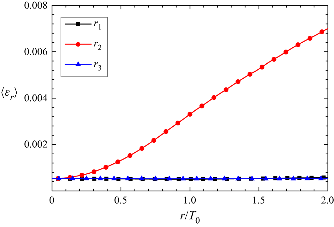
Note that in figure 16, all the terms are normalized by the average pseudo-dissipation  $\langle \varepsilon _r \rangle$. Figure 17 shows the distributions of the dissipation
 $\langle \varepsilon _r \rangle$ along
 $r_1$,
 $r_2$ and
 $r_3$, which gives further information on the homogeneity and isotropy of the scale-by-scale energy cascade. It can be seen that
 $\langle \varepsilon _r \rangle$ is quasi-homogeneous along the streamwise and transverse directions (i.e.
 $r_1$ and
 $r_3$), whereas along the vertical direction,
 $r_2$, the distribution is highly inhomogeneous. The large dissipation for a large separation distance is related to the existence of the energetic dual wakes away from the centreline. By combining figures 16 and 17, one could also draw the conclusion that the two-point energy transfer process is anisotropic at
 $X/T_0=6$.
The averaged two-point pseudo-dissipation  $\langle \varepsilon _r \rangle$ along
 $r_1$,
 $r_2$ and
 $r_3$ at
 $X/T_{0}=6$.

Along  $r_2$ owing to the inhomogeneity of the dual wakes (i.e. considerable variation of the mean velocity) the contribution of the production term cannot be omitted, especially at
 $r_2/T_0 \sim 2$. For a large separation distance (far away from the centreline), which can be deep inside the turbulent wake, the flow fields can be fully turbulent. Consequently, the production term and the dissipation term can be significant. Furthermore, a careful examination of the energy transfer in all three directions reveals that there is no discernible range over which the nonlinear transport term
 $\langle \varPi \rangle$ approximately balances the dissipation term
 $\langle \varepsilon _r \rangle$.
Figure 16(a) shows that a discernible decrease in  $\langle \mathcal {A} \rangle$ can be found in the range
 $r_1 \gtrsim L_{cyc}/2$. For the slowly varied mean streamwise velocity, we may have the approximation
 $2U_1^0 \simeq U_1^{+} + U_1^-$ with
 $U_1^{+} + U_1^- \gg U_2^{+} + U_2^-$ and
 $U_1^{+} + U_1^- \gg U_3^{+} + U_3^-$. Using this relationship, the two-point advection term
 $\langle \mathcal {A} \rangle$ can be rewritten as
 \begin{align} \langle \mathcal{A} \rangle &= \frac{1}{4} (U_j^+ + U_j^-) \left\langle(u_i^+ - u_i^-) \left(\frac{\partial u_i^+ }{\partial X_j^+} - \frac{\partial u_i^- }{\partial X_j^-}\right) \right\rangle \nonumber\\ &\simeq \frac{1}{4} (U_1^+ + U_1^-)\left\langle(u_i^+ - u_i^-) \left( \frac{\partial u_i^+ }{\partial X_1^+} - \frac{\partial u_i^- }{\partial X_1^-}\right) \right\rangle\nonumber\\ &\simeq \frac{1}{2} U_1^0 \left\langle(u_i^+ - u_i^-)\left( \frac{\partial u_i^+ }{\partial X_1^+} - \frac{\partial u_i^- }{\partial X_1^-}\right) \right\rangle\nonumber\\ & = \frac{1}{2} U_1^0\left(\left\langle(u_1^+ - u_1^-)\left( \frac{\partial u_1^+ }{\partial X_1^+} - \frac{\partial u_1^- }{\partial X_1^-}\right) \right\rangle +\left\langle(u_2^+ - u_2^-)\left( \frac{\partial u_2^+ }{\partial X_1^+} - \frac{\partial u_2^- }{\partial X_1^-}\right) \right\rangle\right. \nonumber\\ &\quad\left. +\left\langle(u_3^+ - u_3^-)\left( \frac{\partial u_3^+ }{\partial X_1^+} - \frac{\partial u_3^- }{\partial X_1^-}\right) \right\rangle\right). \end{align}
Both the streamwise and vertical velocity fluctuations  $u_1$ and
 $u_2$ exhibit pronounced frequency spectra peaks at
 $f_s=fT_0/U_{in}\simeq 0.142$ (not shown herein). It might be worth mentioning that the peak frequency of the downstream centreline vertical component
 $u_2$ is half that of the corresponding streamwise component
 $u_1$ downstream of a square cylinder (Portela et al. Reference Portela, Papadakis and Vassilicos2017). Further work involving alternation between the antiphase and inphase vortex shedding from the two square cylinders is required to reveal the physical mechanism of the similar frequency spectra peaks. Thus, we can further neglect the contribution due to the spanwise velocity fluctuation. Owing to the two-dimensional vortex shedding in the
 $X\text {--}Y$ plane the pronounced frequency spectra peaks cannot be found for the spanwise velocity fluctuation
 $u_3$. Consequently, the slow but discernible increase in
 $\langle \mathcal {A} \rangle$ at
 $r_1 \gtrsim L_{cyc}/2$ is related to the repeated two-dimensional large-scale vortex shedding behaviour. It can be also seen from figure 16(a) that two-point energy transfer processes mainly occur within one large-scale vortex shedding cycle.
We now consider the scale-by-scale energy transfer at a far downstream location, i.e.  $X/T_0=26$. Figure 18 shows terms involved in the scale-by-scale energy budget, namely (5.2), along
 $r_1$,
 $r_2$ and
 $r_3$ directions. At the far streamwise location
 $X/T_0=26$, we have
 $\langle \mathcal {A} \rangle + \langle \varPi \rangle \simeq - \langle \varepsilon _r \rangle$ for a relatively short range around
 $r/T_0 \simeq (\lambda /2)/T_0$. This observation is quite different from that at
 $X/T_0=6$, where the dissipation term is much smaller than other non-negligible terms. More specifically, the relation
 $\langle \varPi \rangle \simeq - 0.7 \langle \varepsilon _r \rangle$ in all three directions somewhat echoes Kolmogorov's prediction,
 $\langle \varPi \rangle \simeq - \langle \varepsilon _r \rangle$. The discernible
 $\langle \mathcal {A} \rangle$ may find its roots in the low local Reynolds number (
 $Re_{\lambda }$ is around 100; see figure 2b). According to the local equilibrium hypothesis proposed by Kolmogorov, at sufficiently high Reynolds numbers the variations in the large-scale motions can negligibly affect the small-scale motions, which obviously are not strictly valid at
 $X/T_0=26$. The two transport terms (i.e.
 $\langle \mathcal {T}_u \rangle$ and
 $\langle \mathcal {T}_p \rangle$) are relatively small, implying that the flow becomes more homogeneous, in agreement with the evolution tendency of the one-point energy transfer. The observation that the maximum
 $\langle \varPi \rangle / \langle \varepsilon _r \rangle$ is found at
 $r/T_0 \simeq (\lambda /2)/T_0$ is in accord with the case of decaying homogeneous turbulence (Obligado & Vassilicos Reference Obligado and Vassilicos2019).
The average scale-by-scale energy transfer in (5.5) along (a)  $r_1$, (b)
 $r_2$ and (c)
 $r_3$ at
 $X/T_{0}=26$. All terms are normalized by
 $\langle \varepsilon _r \rangle$. The two vertical dashed lines in (a) correspond to the half-size of the Taylor microscale
 $\lambda /2$ and the half-size of large-scale vortex shedding
 $L_{cyc}/2$, respectively.

It should be stressed that according to Kolmogorov's local equilibrium hypothesis, at a sufficiently high Reynolds number within an extended range there is an instantaneous balance between the dissipation effect and the nonlinear transfer effect, that is, in real space  $\varPi = \varepsilon _r$. Obviously, the statistical balance
 $\langle \varPi \rangle = \langle \varepsilon _r \rangle$ is readily deduced from Kolmogorov's local equilibrium hypothesis. The dimensional analysis for the derivation of the
 $2/3$ power law requires that the flow is in statistical equilibrium (
 $\langle \varPi \rangle = \langle \varepsilon _r \rangle$ holds for a substantial range).
Recently, it has emerged that even at very high Reynolds numbers, the energy cascade process is non-equilibrium (Vassilicos Reference Vassilicos2015) with time lags between  $\varPi$ and
 $\varepsilon _r$ (Goto & Vassilicos Reference Goto and Vassilicos2016) and therefore
 $\varPi \neq \varepsilon _r$. In Obligado & Vassilicos (Reference Obligado and Vassilicos2019), it has been demonstrated in decaying homogeneous isotropic turbulence that the upper end of the inertial range is significantly non-equilibrium and the unsteady term is comparable to the dissipation term. It might be worth stressing that even in a stationary non-equilibrium turbulent flow with high Reynolds number, we should still expect a statistical balance between the temporal-average nonlinear term and the temporal-average dissipation term (e.g. Goto & Vassilicos Reference Goto and Vassilicos2016; Yasuda & Vassilicos Reference Yasuda and Vassilicos2018), that is,
 $\langle \varPi \rangle \simeq \langle \varepsilon _r \rangle$ due to the vanishing unsteady term
 $\langle \mathcal {A}_t^k \rangle$. Therefore, the statistical balance between the time-averaged nonlinear transfer term
 $\langle \varPi \rangle$ and the time-averaged dissipation term
 $\langle \varepsilon _r \rangle$ in stationary turbulence is not necessarily inconsistent with the non-equilibrium phenomenology. It is worth stressing again that the term ‘quasi-Kolmogorov’ in this paper is used for the reason that at
 $X/T_0= 26$ the flow field is more or less homogeneous and isotropic and the exponent of the second-order structure function is close to the expected value, i.e.
 $2/3$, which does not further imply whether the energy cascade process is local equilibrium or not. For the upstream location
 $X/T_0 = 6$, there is no such intermediate separation range where
 $\langle \varPi \rangle$ approximately balances
 $\langle \varepsilon _r \rangle$, and consequently the exponent of the second-order structure function is not
 $2/3$ but a much large value close to 1.
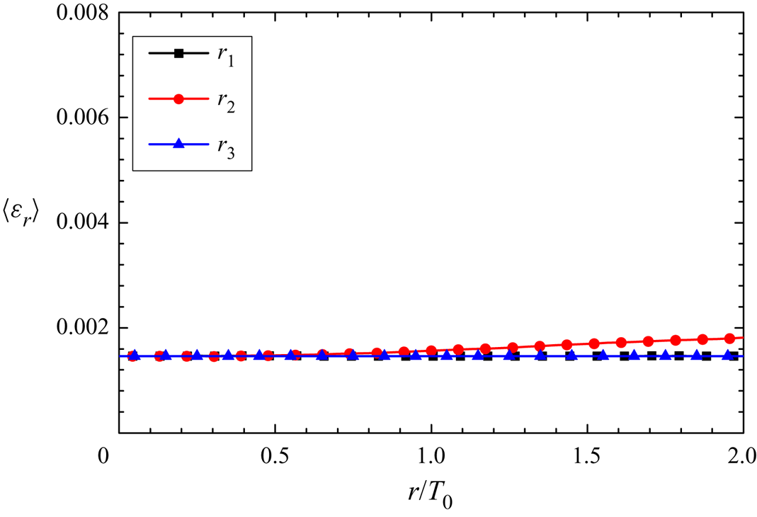
Figure 19 shows the evolution of  $\langle \varepsilon _r \rangle$ along all three directions at
 $X/T_0=26$, which again clearly shows that the degree of homogeneity improves when compared with upstream location
 $X/T_0=6$. By comparing figures 18 and 19, one may draw the conclusion that a reasonably good level of isotropy can be found within the range
 $r/T_0 \lesssim 0.5$. This also reflects a tendency towards isotropization of the dual-wake flow. Along the streamwise direction,
 $r_1$, the cancellation between the pressure transport term
 $\langle \mathcal {T}_p \rangle$ and the turbulent transport term
 $\langle \mathcal {T}_u \rangle$ can be significant at
 $r_1/T_0 \gtrsim 0.5$. It is worth recalling that the small-scale isotropy is a premise for the derivation of Kolmogorov's
 $-5/3$ spectra. The lack of isotropy in the range
 $r/T_0 \gtrsim 0.5$ is related to the persistence of the two wakes.
The averaged two-point pseudo-dissipation  $\langle \varepsilon _r \rangle$ along
 $r_1$,
 $r_2$ and
 $r_3$ at
 $X/T_0=26$.

A short remark concerning the origin of the quasi-Kolmogorov  $-5/3$ spectrum at the far downstream location
 $X/T_0=26$ can be made. First, it has been demonstrated that the corresponding flow becomes fully turbulent,
 $\gamma \simeq 1$. Furthermore, a reasonably good level of homogeneity and isotropy can be reached. Echoing Kolmogorov's prediction, we observe a short range with the relation
 $\langle \varPi \rangle \simeq - 0.7 \langle \varepsilon _r \rangle$, which may explain the discernible power law of the second-order structure with an approximately
 $2/3$ exponent in real space.
The above discussion only focuses on the average the nonlinear transfer along three principal axes (i.e.  $r_1$,
 $r_2$,
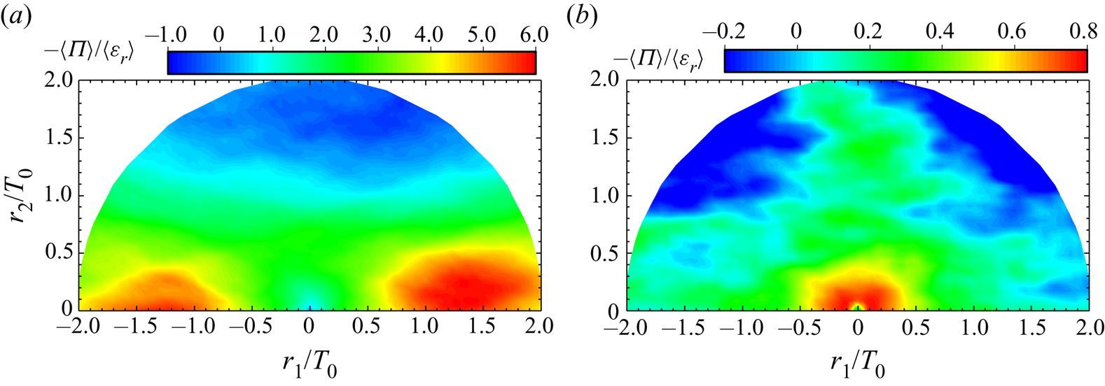
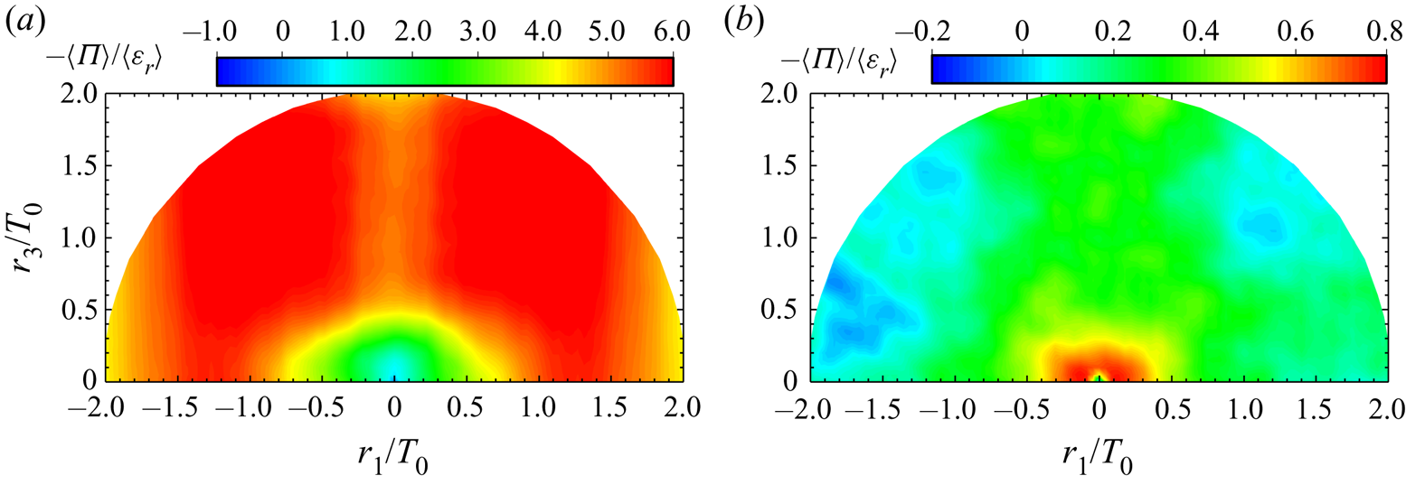
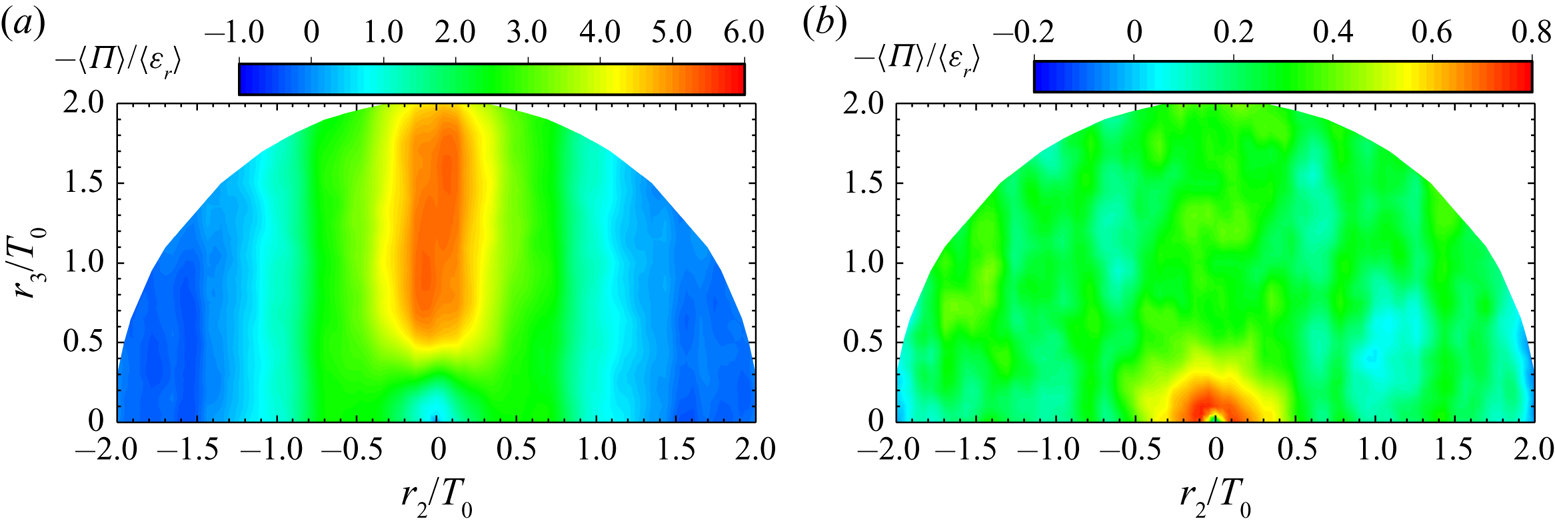
 $r_3$). One should not exclude the possibility that there may exist inverse energy transfer for off-axis directions, especially when considering the fact that in the upstream region the turbulent flow is highly anisotropic. Figures 20–22 show two-dimensional plots of the normalized nonlinear energy transfer term
 $- \langle \varPi \rangle / \langle \varepsilon _r \rangle$ in the
 $(r_1, r_2$),
 $(r_1, r_3)$ and
 $(r_2, r_3)$ planes, respectively. The discernible but small asymmetry in figures 20–22 is related to the finite statistical steps. It can be seen from figures 20–22 that the two-point energy transfer process is highly anisotropic at
 $X/T_0=6$, whereas a reasonably good level of isotropy can be found at the further downstream location
 $X/T_0=26$. Obviously, figures 20–22 indicate that within the range
 $r/T_0 <1.0$, on average the nonlinear terms always serve as source terms at the two locations considered (
 $X/T_0=6$ and 26).
The normalized nonlinear interscale transfer term  $- \langle \varPi \rangle / \langle \varepsilon _r \rangle$ at
 $(a)$
 $X/T_0=6$ and
 $(b)$
 $X/T_0=26$ in the
 $(r_1, r_2)$ plane.

The same as figure 20 but in the  $(r_1, r_3)$ plane.

The same as figure 20 but in the  $(r_2, r_3)$ plane.

5.3. Relation between one-point and two-point energy transfer
It is well known that the one-point energy balance is related to the exchange of energy between the mean and fluctuating fields, whereas the two-point energy balance reflects the energy exchanges between different scales of motions. As the separation distance  $\boldsymbol {r}$ approaches a zero vector, the only two remaining terms in the KHMH equation are
 $\langle \mathcal {D}_r \rangle$ and
 $\langle \varepsilon _r \rangle$, that is,
 $\langle \mathcal {D}_r \rangle = \langle \varepsilon _r \rangle$. On the other hand, when
 $\boldsymbol {r}$ is sufficiently large, the velocities at the two spatial points considered could be uncorrelated. And by further assuming the flow is homogeneous, the asymptotic form of the KHMH equation, namely (5.1), simply reduces to four times the one-point energy budget, namely (4.1).
It can be seen by comparing figures 9, 16 and 18 that the behaviour of the one-point energy balance closely resembles that of the two-point energy balance over significant intermediate separation scales, which is perhaps much less noticed. The first evidence is related to the relative importance of the viscous dissipation (i.e.  $\langle \varepsilon ^k_r \rangle$ and
 $\langle \varepsilon _r \rangle$). In the upstream region
 $X/T_0=6$ the contributions of the dissipation are small in both one- and two-point energy transfer, whilst at
 $X/T_0=26$ the dissipation effects are responsible for the major loss of
 $\langle k \rangle$ and
 $\langle \delta q^2 \rangle$. This observation is partially related to the small difference between the one-point ‘true’ dissipation and the one-point pseudo-dissipation. As can be seen from figure 23, the two profiles virtually collapse together. The second point is that the impacts of the non-negligible terms in the one-point energy budget and their two-points counterparts, i.e. (
 $\langle \mathcal {T}_p^k \rangle$,
 $\langle \mathcal {T}_p \rangle$), (
 $\langle \mathcal {T}_u^k \rangle$,
 $\langle \mathcal {T}_u \rangle$) and (
 $\langle \mathcal {A}^k \rangle$,
 $\langle \mathcal {A} \rangle$), are similar in terms of being a source or sink term. For instance, at
 $X/T_0=6$ the time-averaged pressure term
 $\langle \mathcal {T}_p^k \rangle$ is negative in the one-point energy balance, and within a considerably intermediate range along all three directions, the pressure term
 $\langle \mathcal {T}_p \rangle$ in the two-point energy transfer is also negative. This observation indicates that the pressure-related terms (i.e.
 $\langle \mathcal {T}_p^k \rangle$ and
 $\langle \mathcal {T}_p \rangle$) contribute to a loss of the one-point kinetic energy
 $\langle k\rangle$ and the two-point second-order structure function
 $\langle \delta q^2\rangle$. Besides the two pressure transport terms (
 $\langle \mathcal {T}_p^k \rangle$ and
 $\langle \mathcal {T}_p \rangle$), the advection terms (i.e.
 $\langle \mathcal {A}^k \rangle$ and
 $\langle \mathcal {A} \rangle$) and turbulent transport terms (i.e.
 $\langle \mathcal {T}_u^k \rangle$ and
 $\langle \mathcal {T}_u \rangle$) also exhibit similar influences (in terms of gain or loss) on
 $\langle k\rangle$ and
 $\langle \delta q^2\rangle$.
Streamwise evolution of the one-point ‘true’ dissipation and one-point pseudo-dissipation along the centreline. The two vertical dashed lines indicate  $X/T_0=6$ and 26, respectively.

To investigate the intrinsic correlation between the one-point and two-point energy transfers, we start from the pressure transport effects. The one-point and two-point pressure transport terms are
 \begin{align} \langle \mathcal{T}_p^k \rangle =- \left\langle u_{i} \frac{\partial}{\partial X_{i}} p \right\rangle\quad \textrm{and} \quad 4 \langle \mathcal{T}_p \rangle = -2\left\langle u_i^+\frac{\partial p^+}{\partial X_{i}^+} +u_i^-\frac{\partial p^-}{\partial X_{i}^-} - u_i^-\frac{\partial p^+}{\partial X_{i}^+} - u_i^+\frac{\partial p^-}{\partial X_{i}^-} \right\rangle, \end{align}
respectively. A little algebra leaves us with
 \begin{align} 4\langle \mathcal{T}_p \rangle &= -2\left\langle u_k^+\frac{\partial p^+}{\partial X_{k}^+} \right\rangle\left(1 - \left.\left\langle u_i^-\frac{\partial p^+}{\partial X_{i}^+} \right\rangle \right/ \left\langle u_j^+\frac{\partial p^+}{\partial X_{j}^+} \right\rangle\right)\nonumber\\ &\quad -2\left\langle u_k^-\frac{\partial p^-}{\partial X_{k}^-}\right\rangle\left(1 - \left.\left\langle u_i^+\frac{\partial p^-}{\partial X_{i}^-} \right\rangle\right/\left\langle u_j^-\frac{\partial p^-}{\partial X_{j}^-}\right\rangle\right) \nonumber\\ & = -2\left\langle u_i^+\frac{\partial p^+}{\partial X_{i}^+} \right\rangle\left(1-f\left(\boldsymbol{X}^-,\boldsymbol{X}^+\right)\right) -2\left\langle u_i^-\frac{\partial p^-}{\partial X_{i}^-} \right\rangle\left(1-f\left(\boldsymbol{X}^+,\boldsymbol{X}^-\right)\right). \end{align}
Clearly,
 \begin{equation} f(\boldsymbol{X}^-,\boldsymbol{X}^+)=\left. \left\langle u_i^-\frac{\partial p^+}{\partial X_{i}^+} \right\rangle \right/ \left\langle u_j^+\frac{\partial p^+}{\partial X_{j}^+} \right\rangle \end{equation}
is a quasi two-point spatial correlation function, which is equal to one if  $X^+=X^-$ and approaches zero in the limit
 $|X^+-X^-| \to \infty$. It must be noted that the quasi two-point correlation function
 $f$ should not be confused with the correlation coefficient
 $\rho$ used in § 4. Within an intermediate separation range,
 \begin{equation} -\left\langle u_i^+\frac{\partial p^+}{\partial X_{i}^+} \right\rangle\quad \textrm{and}\quad -\left\langle u_i^-\frac{\partial p^-}{\partial X_{i}^-} \right\rangle \end{equation}
take the same sign and the two-point spatial correlation  $f(\boldsymbol {X}^-,\boldsymbol {X}^+)$ (also
 $f(\boldsymbol {X}^+,\boldsymbol {X}^-)$) tends to take a positive value, which is smaller than 1. One may also expect that the signs of the one-point
 $\langle \mathcal {T}_p^k \rangle$ and the two-point
 $\langle \mathcal {T}_p \rangle$ for an intermediate separation are the same. Similar conclusions can also be reached for other related terms.
Before closing this section, we make a short remark concerning the two-point energy exchanges at  $X/T_0=6$, where the flow is highly intermittent, significantly inhomogeneous/anisotropic with the appearance of a well-defined
 $-5/3$ energy spectrum. The simplified KHMH equation is
 $\langle \mathcal {A} \rangle + \langle \varPi \rangle \simeq \langle \mathcal {T}_u \rangle + \langle \mathcal {T}_p \rangle - \langle \varepsilon _r\rangle$ within a significant separation range. This observation clearly violates Kolmogorov's equilibrium predictions. The active roles of the advection, turbulent transport and pressure transport terms (i.e.
 $\langle \mathcal {A} \rangle$,
 $\langle \mathcal {T}_u \rangle$ and
 $\langle \mathcal {T}_p \rangle$) may find their roots in the one-point energy budget.
6. Conclusion
The current work represents a continuation of our previous investigation of turbulent flows behind two side-by-side square cylinders. We first decompose the streamwise velocity fluctuations  $u_1$ into two parts (spanwise average part
 $u_1^m$ and the residual part
 $u_1^r$), that is,
 $u_1=u_1^m+u_1^r$. The background part
 $u_1^m$ contributes to the low-frequency range of the spectrum of
 $u_1$, whereas the residual part
 $u_1^r$ is a direct cause of the non-Kolmogorov
 $-5/3$ spectrum at
 $X/T_0=6$.
As a further step towards better understanding of the energy transfer mechanisms, we investigate the streamwise evolution of the one-point turbulent kinetic energy budget and also the two-point energy budget at two centreline locations, namely an upstream location  $X/T_0=6$ and a further downstream location
 $X/T_0=26$, by resorting to the generalized Kármán–Howarth equation. Based on the intermittency factor
 $\gamma$, the flow field can be approximately divided into three different subregions (i.e. laminar/irrotational region, intermittent region and fully turbulent region). The first finding is that the features of the one-point energy transfer are significantly different in different flow regions. At
 $X/T_0 = 6$ the sweeping effect can be noticeable because of the energetic quasi-periodic/regular oscillations, whereas at
 $X/T_0 = 26$ the sweeping effect is quite small. In contrast, persistent significant negative correlation between
 $\mathcal {T}_p^k$ and
 $\mathcal {T}_u^k$ can be found owing to the non-locality of incompressible turbulent flows (i.e.
 $\boldsymbol {\nabla } \boldsymbol {\cdot }(\boldsymbol {u} \boldsymbol {\cdot } \boldsymbol {\nabla } \boldsymbol {u})=-\nabla ^{2} P$).
At the upstream location  $X/T_0=6$, where the flow is highly intermittent, the scale-by-scale energy cascade is highly inhomogeneous and anisotropic and the KHMH equation cannot reduce to the well-known statistical balance relation, namely
 $\langle \varPi \rangle \simeq - \langle \varepsilon _r \rangle$. Instead, within significant intermediate ranges in all three directions, the KHMH approximation that we are faced with is
 $\langle \mathcal {A} \rangle + \langle \varPi \rangle \simeq \langle \mathcal {T}_u \rangle + \langle \mathcal {T}_p \rangle - \langle \varepsilon _r\rangle .$ Moreover, the magnitude of the average viscous dissipation term
 $\langle \varepsilon _r\rangle$ is much smaller than other non-negligible terms. In other words, the roles of the advection, non-local pressure, nonlinear transport and turbulent transport terms in the scale-by-scale energy transfer are significantly important, which clearly violates Kolmogorov's equilibrium predictions. In the downstream region (i.e.
 $X/T_0=26$), where the dual-wake flow is almost fully turbulent and becomes much more homogeneous and isotropic, within short intermediate ranges the simplified two-point energy budget is
 $\langle \mathcal {A} \rangle + \langle \varPi \rangle \simeq - \langle \varepsilon _r \rangle$, which is close to Kolmogorov's prediction, namely
 $\langle \varPi \rangle \simeq - \langle \varepsilon _r \rangle$.
The non-vanishing advection term (i.e.  $\langle \mathcal {A} \rangle \simeq - 0.3 \langle \varepsilon _r \rangle$) is probably caused by the relatively low local Reynolds number, which implies that the time scales of
 $\langle \varPi \rangle$ and
 $\langle \varepsilon _r \rangle$ are not sufficiently small when compared with that of the large-scale advection
 $\langle \mathcal {A} \rangle$. By comparing the behaviour of the one-point and two-point energy transfer at
 $X/T_0=6$ and 26, it can be seen that the two different energy transfer processes are actually closely related, that is, similar relative importance of the viscous dissipation and the same role of the non-negligible terms in terms of being source term or sink term.
In the upstream region (i.e.  $X/T_0=6$), the flow field is highly intermittent with bursts of extreme events. The correlation between extreme events and the vortex shedding behaviour (i.e. sinuous mode or varicose mode and the switch between the two modes) in such intermittent flow region is an important remaining issue, which should be pursued in future work. The conditional analysis for the energy transfer processes, for example, scale-by-scale energy transfer based on the states of two separation points (including three different cases: laminar–laminar, laminar–turbulent and turbulent–turbulent states), in the intermittent flow region would be another important research topic.
Acknowledgements
This work was in part supported by the National Natural Science Foundation of China (nos. 91952105 and 11802133), the Natural Science Foundation of Jiangsu Province (no. BK20180454) and the Fundamental Research Funds for the Central Universities (no. 30918011325). Part of this study was also supported by MEXT KAKENHI (nos. 18H01367 and 18H01369). Part of the numerical simulations were carried out on the supercomputer at Tohoku University (nos. J18I078 and J19I100: Institute of Fluid Science, Tohoku University; and no. CP02APR18: Advanced Fluid Information Research Center, Institute of Fluid Science, Tohoku University). The authors acknowledge the helpful discussions with Dr J. C. Vassilicos (Lille Fluid Mechanics Laboratory–Kampé de Fériet, Lille, France). We are also grateful to the anonymous referees for their valuable comments.
Declaration of interests
The authors report no conflict of interest.