2. Problem formulation

We consider a rigid, spherical autophoretic particle of radius $a^{*}$ in an incompressible Newtonian fluid of viscosity $\eta ^{*}$, whose flow obeys the Stokes equations. Above and henceforth, dimensional variables are marked with an asterisk as superscript. There is a constant flux $\mathcal {A}^{*}$ of solute at the particle surface, which is positive (negative) when the solute is being emitted (absorbed) at the interface. Far away from the particle, the uniform solute concentration is $C^{*}_{\infty }$, and the difference between the local concentration and its far-field value is denoted by $c^{*}=C^{*}-C^{*}_{\infty }$. The solute molecules, of diffusivity $D^{*}$, interact with the active particle via a short-ranged potential whose characteristic length is $b^{*}$, such that $b^{*}\ll a^{*}$. These interactions give rise to a tangential slip velocity along the particle surface (Anderson Reference Anderson1989), whose magnitude is set by the concentration gradient of the solute at the interface, and the mobility parameter, $\mathcal {M}^{*}=\pm {k_B^{*}T^{*}b^{*2}}/{\eta ^{*}}$, where $k^{*}_{B}$ is Boltzmann's constant and $T^{*}$ is the absolute temperature. Attractive (repulsive) interactions between the solute and the active particle are described by a negative (positive) $\mathcal {M}^{*}$ (Michelin & Lauga Reference Michelin and Lauga2014). The concentration profile of the solute, therefore, evolves due to diffusion and advection by fluid flow.

Following Michelin et al. (Reference Michelin, Lauga and Bartolo2013), length, time, fluid velocity, pressure and concentration are scaled by $a^{*}$, ${a^{*}D^{*}}/{|\mathcal {A}^{*}\mathcal {M}^{*}|}$, $U^*={|\mathcal {A}^{*}\mathcal {M}^{*}|}/{D^{*}}$, ${\eta ^{*}U^*}/{a^{*}}$ and ${a^{*}|\mathcal {A}^{*}|}/{D^{*}}$, respectively. Additionally, following Saha et al. (Reference Saha, Yariv and Schnitzer2021) an external force of magnitude $F^*$ imposed on the particle leads to a ‘mechanical’ velocity scale $W^*=F^*/(6{\rm \pi} \eta ^*a^*)$. In the subsequent discussion, variables without asterisks are the dimensionless equivalent of their dimensional counterparts. A key dimensionless parameter is the intrinsic Péclet number,

(2.1)\begin{equation} Pe=\dfrac{a^{*}|\mathcal{A}^{*}\mathcal{M}^{*}|}{D^{*2}}, \end{equation}

which quantifies the relative importance of the solute advection with respect to its diffusion, and is a measure of the chemical activity of the particle. Another important parameter is the ratio of ‘mechanical’ to ‘chemical’ velocity scales, $\epsilon =W^*/U^*$, which is by assumption small compared with unity in the work of Saha et al. (Reference Saha, Yariv and Schnitzer2021). It is convenient to introduce the scaled flux and mobility parameters

(2.2a,b)\begin{equation} A=\dfrac{\mathcal{A}^{*}}{|\mathcal{A}^{*}|}, \quad M=\dfrac{\mathcal{M}^{*}}{|\mathcal{M}^{*}|}. \end{equation}

The concentration field is governed by the unsteady advection–diffusion equation

(2.3)\begin{equation} Pe\left(\dfrac{\partial c}{\partial t}+\boldsymbol{v} \boldsymbol{\cdot}\boldsymbol{\nabla} c\right)=\nabla^2 c, \end{equation}

where $t$ is time and $\boldsymbol {v}$ denotes the velocity field. Equation (2.3) is subject to the two boundary conditions of: (i) constant flux of the solute at the surface of the active particle

(2.4)\begin{equation} \dfrac{\partial c}{\partial r}={-}A\text{ at } r=1, \end{equation}

and (ii) an attenuation condition far away from the particle

(2.5)\begin{equation} c\to0\text{ as } r\to\infty. \end{equation}

We employ a cylindrical coordinate system $(z,\rho,\phi )$ with its origin attached to the particle centre. The $z$-axis represents the axis of symmetry along which the particle motion is constrained. The perpendicular distance from the $z$-axis is measured by the $\rho$-coordinate, and $\phi$ denotes the azimuthal angle of rotation about the $z$-axis. This frame of reference is non-inertial since the particle is accelerating during its unsteady translation. However, this choice does not affect the advection–diffusion equation or the fluid flow equations, since the motion occurs at zero Reynolds number. The particle surface is denoted by $r=1$ where $r=\sqrt {\rho ^2+z^2}$. The axisymmetric flow around the particle is represented as

(2.6)\begin{equation} \boldsymbol{v}={v}_{z}(\rho,z)\boldsymbol{e}_{z}+{v}_{\rho} (\rho,z)\boldsymbol{e}_{\rho}, \end{equation}

where $\boldsymbol {e}_{z}$ and $\boldsymbol {e}_{\rho }$ are unit vectors along the $z$ and $\rho$ axes, respectively. It is useful to define the polar angle $\theta \equiv \arctan (\rho /z)$ measured anticlockwise such that $\theta =0$ lies on the positive $z$-axis.

The velocity field, $\boldsymbol {v}$, in (2.3) is governed by the incompressibility criterion and the Stokes equation

(2.7a,b)\begin{equation} \boldsymbol{\nabla}\boldsymbol{\cdot}\boldsymbol{v}=0, \quad \nabla^2\boldsymbol{v}=\boldsymbol{\nabla} p, \end{equation}

where $p$ is the dynamic pressure, and subject to the following boundary conditions:

(2.8)\begin{equation} \boldsymbol{v}\equiv M\boldsymbol{\nabla}_{{s}}c=v_{{s}} (\cos\theta\boldsymbol{e}_{\rho}-\sin\theta\boldsymbol{e}_{z}) \text{ at } r=1, \end{equation}

where

(2.9)\begin{equation} v_{{s}}=M\left(\cos\theta\dfrac{\partial c}{\partial \rho}- \sin\theta\dfrac{\partial c}{\partial z}\right), \end{equation}

and

(2.10)\begin{equation} \boldsymbol{v}\to-U\boldsymbol{e}_{z}\text{ as } r\to\infty. \end{equation}

The far-field speed $U$ in (2.10) is unknown a priori, and is determined by requiring that the total hydrodynamic force on the particle in the $z$-direction is at all times is equal to $-6{\rm \pi} \epsilon$. The presumed axisymmetry of the problem permits us to rewrite the velocity field in terms of the Stokes streamfunction $\psi$

(2.11)\begin{equation} \boldsymbol{v}=\dfrac{1}{\rho}\left(\boldsymbol{e}_{z} \dfrac{\partial \psi}{\partial \rho}-\boldsymbol{e}_{\rho} \dfrac{\partial \psi}{\partial z}\right)\equiv \dfrac{1}{\rho}{\nabla}^{{\perp}}\psi. \end{equation}

Taking the curl of the Stokes equations and introducing the vorticity vector $\boldsymbol {\omega }=\boldsymbol {\nabla }\times \boldsymbol {v}$ eliminates the pressure from the governing equations, resulting in the following system of coupled partial differential equations:

(2.12)$$\begin{gather} \omega\rho+E^2\psi=0, \end{gather}$$

(2.13)$$\begin{gather}\nabla^2 \omega-\dfrac{\omega}{\rho^2}=0, \end{gather}$$

where $\omega$ is the $\phi$-component of the vorticity $\boldsymbol {\omega }$ about the $z$-axis, with the other components ($\rho$ and $z$) of the vorticity vector vanishing due to symmetry, and the operators

(2.14a,b)\begin{equation} \nabla^2=\dfrac{1}{\rho}\dfrac{\partial}{\partial \rho} \left(\rho\dfrac{\partial}{\partial \rho}\right)+ \dfrac{\partial^2}{\partial z^2},\quad E^2=\nabla^2-\dfrac{2}{\rho}\dfrac{\partial}{\partial \rho}. \end{equation}

Equations (2.12) and (2.13) must be solved subject to the following boundary conditions:

(2.15)$$\begin{gather} \boldsymbol{n}\boldsymbol{\cdot}\boldsymbol{\nabla}\psi={-}\rho v_{{s}} \text{ at } r=1, \end{gather}$$

(2.16)$$\begin{gather}\boldsymbol{n}\boldsymbol{\cdot}\boldsymbol{\nabla}\psi\to-\rho U\sin\theta \text{ as } r\to\infty, \end{gather}$$

(2.17)$$\begin{gather}\boldsymbol{n}\boldsymbol{\cdot}\boldsymbol{\nabla}\omega\to0 \text{ as } r\to\infty, \end{gather}$$

(2.18)$$\begin{gather}\psi=0\text{ at } r=1, \end{gather}$$

with $\boldsymbol {n}=\cos \theta \boldsymbol {e}_{z}+\sin \theta \boldsymbol {e}_{\rho }$ being the unit normal to the particle surface pointing into the fluid; and the symmetry condition

(2.19)\begin{equation} \psi=\omega=0\text{ along } \rho=0. \end{equation}

For an unforced particle ($\epsilon =0$) there exists a trivial solution to the system of (2.3), (2.12) and (2.13), which is the isotropic concentration profile $c=1/r$, corresponding to the quiescent state of zero phoretic velocity and no fluid motion at all times. Beyond $Pe=4$, however, the quiescent state becomes unstable with respect to dipolar perturbations in the concentration field (Michelin et al. Reference Michelin, Lauga and Bartolo2013; Morozov & Michelin Reference Morozov and Michelin2019), and the autophoretic particle sets into motion. Further types of perturbation (such as quadrupolar) are unstable at larger values of the Péclet number as the higher hydrodynamic modes are excited. We therefore supply an asymmetrical concentration field as the initial condition to (2.3), as follows:

(2.20)\begin{equation} c(r,t=0)=\dfrac{1}{r}-\delta_{{per}}\left(\dfrac{\cos\theta}{r^2}\right), \end{equation}

with $|\delta _{{per}}|<1$.

For a forced particle ($\epsilon \neq 0$), there exists no trivial solution corresponding to an isotropic concentration profile. Nonetheless, we still use an initial condition of the form given by (2.20). The agreement of the resultant numerical results with the asymptotic predictions of Saha et al. (Reference Saha, Yariv and Schnitzer2021) (discussed in § 5) justifies the use of this initial condition.

3. Numerical solution methodology

Numerical computations require the stipulation of a finite outer boundary, and a value of $R_{{o}}=100$ is chosen as the radius of the spherical shell on which the far-field boundary conditions are prescribed, unless specified otherwise. The far-field boundary conditions, (2.5) and (2.10), are enforced exactly at $r=R_{{o}}$. The computational domain is a polar grid in the $(r,\theta )$ space, with $N_{r}=N_{\theta }=15$ quadrilateral elements in both the radial and angular directions. The elements in the $\theta -$ direction are evenly spaced in the range $[0,{\rm \pi} ]$, while those in the $r$-direction are arranged such that the size of the radial elements follow a geometrical progression, with the width of the radial element closest to the particle surface being $\Delta r_{0}=0.388$.

As the first step in the numerical solution process, the initial condition given in (2.20) is used to specify the slip boundary condition (2.8) for the flow problem. The self-propulsion speed $U(t)$ at any instant of time $t$ must satisfy the requirement that the total hydrodynamic drag force on the particle in the $z$-direction, $F_{z}$, given by (Khair & Chisholm Reference Khair and Chisholm2014)

(3.1)\begin{equation} F_{z}=\left\{{\rm \pi}\int_{0}^{\rm \pi}\left[\dfrac{\partial(\omega r)}{\partial r}-2\omega\right]_{r=1}\sin^2\theta\, {\rm d}\theta\right\}+6{\rm \pi}\epsilon, \end{equation}

vanishes at $t$. The self-propulsion speed is evaluated iteratively using a secant method, as described in Chisholm et al. (Reference Chisholm, Legendre, Lauga and Khair2016). Given two initial guesses $U^{\langle \ell \rangle }$ and $U^{\langle \ell -1\rangle }$ at time $t$, where $\ell$ denotes the iteration number, the hydrodynamic drag at the two values of the self-propulsion speed are evaluated. Using linear interpolation, an improved estimate for $U$ is obtained as $U^{\langle \ell +1\rangle }=(U^{\langle \ell \rangle }F_z^{\langle \ell -1\rangle }-U^{\langle \ell -1\rangle }F_z^{\langle \ell \rangle })/(F_z^{\langle \ell -1\rangle }-F_z^{\langle \ell \rangle })$. The procedure is terminated when the magnitude of the difference in the computed speeds between successive iterations $|U^{\langle \ell \rangle }-U^{\langle \ell -1\rangle }|$ is reduced below $10^{-5}$. The converged solution for the flow field $(\psi,\omega )$ at each time instant is then used to solve the advection–diffusion equation for the concentration field. We present next the algorithm for the solution of the advection–diffusion equation governing the transient evolution of concentration (2.3). The Stokes equations governing the flow field are solved in the same manner as in Chisholm et al. (Reference Chisholm, Legendre, Lauga and Khair2016) and Khair & Chisholm (Reference Khair and Chisholm2018).

The time derivative in (2.3) is discretized using the finite-difference formula

(3.2)\begin{equation} \dfrac{\partial c}{\partial t}\approx \dfrac{c^{(n+1)}-c^{(n)}}{\Delta t}, \end{equation}

where $c^{(n)}$ denotes the value of the concentration at the discrete time $t^{(i)}$, and $\Delta t\equiv t^{(n+1)}-t^{(n)}$ is the width of the discrete timestep.

The concentration variable is taken to be the weighted sum of its values at its current and previous timestep, that is,

(3.3)\begin{equation} c=\varTheta c^{(n+1)}+(1-\varTheta)c^{(n)}, \end{equation}

where the choice of the $\varTheta$ parameter corresponds to different well-known methods for time discretization. For example, $\varTheta =1$ represents the backward Euler method, while $\varTheta =1/2$ is used in the Crank–Nicolson algorithm. We have used the latter method throughout this paper, in view of its unconditional stability and second-order accuracy (Tanaka, Matsumoto & Yang Reference Tanaka, Matsumoto and Yang1994; Donea & Huerta Reference Donea and Huerta2003) with respect to the discretization width, $\Delta t$. A value of $\Delta t=1.0$ is used for simulations with $Pe<20$, while a timestep width of 0.1 is used at higher values of the Péclet number. In the discussion that follows, we have retained the $\varTheta$ notation for the sake of generality.

Substituting (3.2) into (2.3), the governing equation may be rewritten as

(3.4) \begin{equation} \left.\begin{array}{c@{}} -(\varTheta\Delta t)\nabla^2c^{(n+1)}+{Pe} c^{(n+1)}+{Pe}(\varTheta\Delta t) (\boldsymbol{v}\,{\cdot}\,{\boldsymbol{\nabla}}c^{(n+1)})\\ -(1-\varTheta)\Delta t\nabla^2c^{(n)}-{Pe} c^{(n)}+{Pe}\Delta t(1-\varTheta) (\boldsymbol{v}\,{\cdot}\,{\boldsymbol{\nabla}}c^{(n)})=0 \end{array}\right\}, \end{equation}

where the velocity $\boldsymbol {v}$ is known from the solution of (2.12) and (2.13). The weak variational form of (3.4) is obtained by multiplying each term by a test function and taking an inner product (Khair & Chisholm Reference Khair and Chisholm2018; Campion–Renson & Crochet Reference Campion–Renson and Crochet1978). The concentration field is discretized, and the independent variables ($\rho,z$) parametrized using a set of shape functions defined as tensor products of 1-D Lagrange polynomials of high order ($N_{{o}}=8$), supported at $N_{{o}}+1$ Gauss–Lobatto quadrature points over the standard region $[-1,1]^2$. 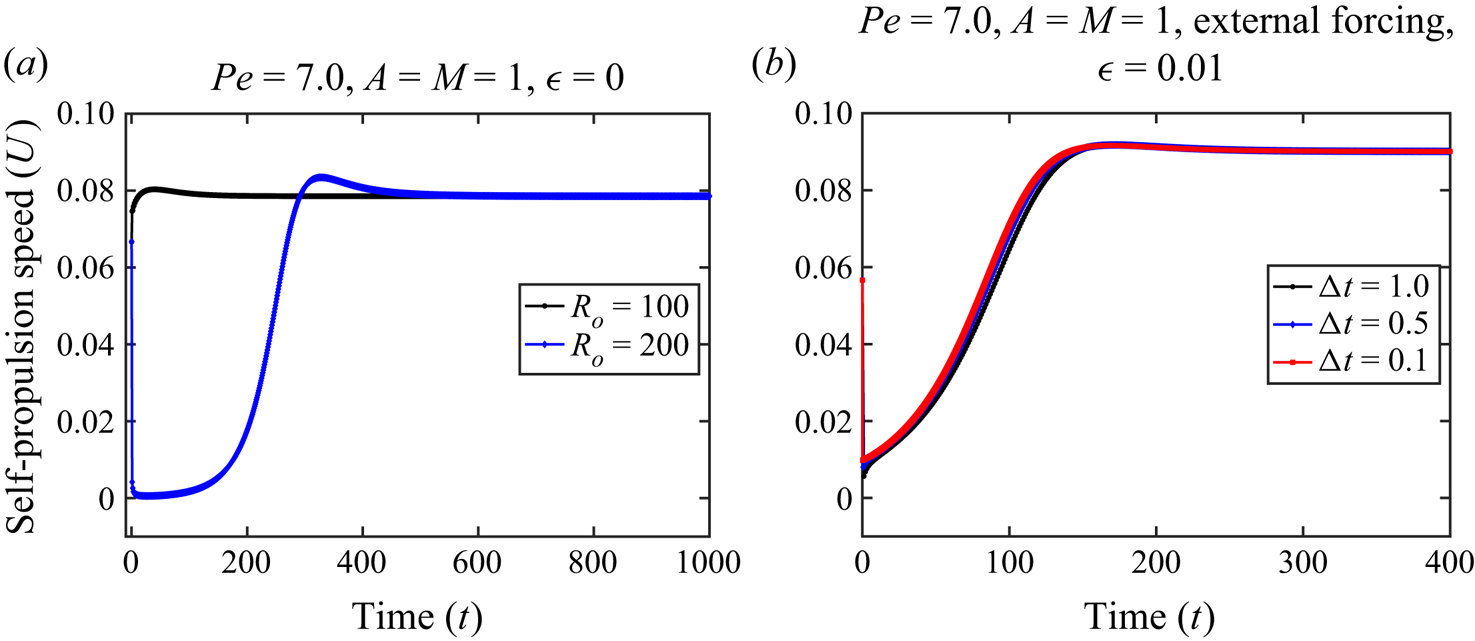A global matrix equation over all spectral elements is then assembled, and solved iteratively until the $L^2$-norm of the difference in concentration between successive iterations computed over all discretization points at each timestep drops below $10^{-6}$. Convergence studies with respect to the outer shell radius ($R_{o}$) and the integration timestep ($\Delta t$) are provided in the Appendix.

Previous investigations (Michelin et al. Reference Michelin, Lauga and Bartolo2013; Hu et al. Reference Hu, Lin, Rafai and Misbah2019) on autophoresis have established that for unforced particles ($\epsilon =0$) with oppositely signed $A$ and $M$, perturbations to the concentration field vanish in the long-time limit, where the particle remains stationary. We therefore concern ourselves with the non-trivial case of similarly signed $A$ and $M$ values, which results in the self-propulsion of the particle, and we pick $A=M=1$ without loss of generality. We examine both $AM=1$ and $AM=-1$ for a forced particle.

At $Pe\leq 10$ the solver is supplied an initial condition of the form given by (2.20), with the choice of $\delta _{{per}}=0.1$. It is observed that different values of $\delta _{{per}}$ in this regime result in the same long-time prediction for the steady phoretic velocity. At $Pe>10$ the concentration profile computed at a previous (lower) value of the Péclet number is used as the initial condition for the subsequent simulation at the next higher Pe.

The transient solver for the concentration field described above may be used across a range of $Pe$, because it does not make any assumptions about the steadiness of the self-propulsion, and thereby allows for the phoretic velocity and the concentration field to be functions of time. An alternative solution methodology, valid (and more efficient) at low values of $Pe$, where the particle is either stationary or undergoing steady translation, is an iterative technique, which solves the coupled system of equations given by the steady advection–diffusion equation

(3.5)\begin{equation} Pe(\boldsymbol{v}\boldsymbol{\cdot}\boldsymbol{\nabla} c)=\nabla^2 c, \end{equation}

and (2.7a,b), using the spectral element method, and subject to the same boundary conditions as described previously. The calculation is started by providing a concentration field of the form given by the right-hand side of (2.20) as the initial guess, and repeated until the difference between the phoretic velocities obtained in successive iterations differ by less than $10^{-5}$. The utility of the iterative solver is admittedly limited in comparison with the transient solver. 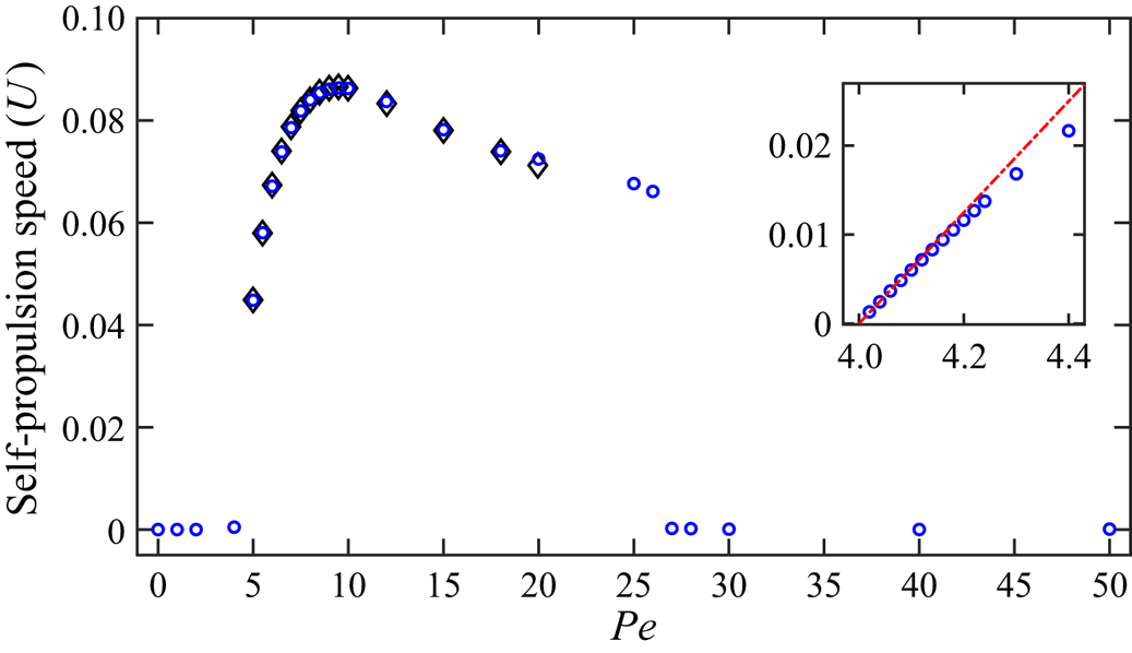Nonetheless, the results obtained using the iterative solver prove useful in comparison against analytical approximations for the self-propulsion speed of unforced and forced autophoretic particles near $Pe=4$, as discussed below in connection with figures 1 and 9. All results presented henceforth in this paper have been obtained using the transient solver, unless mentioned otherwise.

Figure 1.

Steady self-propulsion speed of an unforced autophoretic particle at various Péclet numbers across the quiescent, steady and stirring regimes. The unfilled diamonds ($\diamond$) represent results obtained by Michelin et al. (Reference Michelin, Lauga and Bartolo2013), and the unfilled circles are from the present work. The inset compares the numerical results obtained using the iterative solver with $R_o=1000$ in the vicinity of the first bifurcation against the analytical approximation, $U=(Pe-4)/16$ (indicated by line), derived by Morozov & Michelin (Reference Morozov and Michelin2019) and Saha et al. (Reference Saha, Yariv and Schnitzer2021).

The axisymmetry of the flow field restricts motion of the particle along the $z$ axis. From the computed time series of the self-propulsion speed, the particle position at a discrete time $i+1$ is evaluated as

(3.6)\begin{equation} z({i+1})=z({i})+U(i)\Delta t;\quad z(0)=0. \end{equation}

In the time interval $[0,t_{{sim}}]$, a total of $N\equiv t_{{sim}}/\Delta t$ data points are recorded. The MSD and VAC, $C_v$, at the $n$th time interval are evaluated as follows:

(3.7)$$\begin{gather} {MSD}(n)=\dfrac{1}{N-n}\sum_{i=0}^{N-n} [z(i+n)-z(i)]^2, \end{gather}$$

(3.8)$$\begin{gather}C_{v}(n)=\dfrac{1}{N-n}\sum_{i=0}^{N-n} [\boldsymbol{e}_{u}(i+n)\boldsymbol{\cdot}\boldsymbol{e}_{u}(i)], \end{gather}$$

where $\boldsymbol {e}_{u}(i)\equiv U(i)/|U(i)|$ is the unit direction vector of the self-propulsion speed at discrete time $i$, and can take the value of $+1$ or $-1$. Equations (3.7) and (3.8) represent calculations of the time average over a single trajectory. The lag time is defined as $\tau \equiv n\Delta t$ and used in reporting the MSD and VAC results. For $Pe\geq 50$, the total simulation time is at least $t_{{sim}}=5\times 10^3$, while those for $Pe=75$ and $Pe=80$ are $t_{{sim}}=1\times 10^4$ and $t_{{sim}}=2\times 10^4$, respectively. Data points corresponding to at least the first $1\times 10^4$ timesteps in these runs are discarded prior to the calculation of the MSD and VAC, to remove the effects of transients.

4. Unforced autophoretic particle

We analyse the dynamics of the autophoretic particle as a function of the Péclet number. Michelin et al. (Reference Michelin, Lauga and Bartolo2013) have shown that the particle remains stationary until a critical Péclet number, $Pe_{{c}}=4$. This range, $0\leq Pe \leq 4$, may be termed as the quiescent regime. As the Péclet number is increased beyond 4, the fore–aft symmetry in the concentration profile is broken, and the particle executes steady rectilinear self-propulsion. In figure 1, the steady self-propulsion speed $U$ from our computations is plotted as a function of Pe, and it is seen that $U$ attains a maximum at $Pe\approx 9$, and decreases smoothly up to a value of $Pe\approx 26$. This range, $4< Pe\leq 26$, is classified as the steady self-propulsion regime. The good agreement of our results with data from Michelin et al. (Reference Michelin, Lauga and Bartolo2013) lends confidence to the numerical procedure used in the present work.

In the inset to figure 1, the self-propulsion speed in the vicinity of symmetry breaking is plotted as a function of $Pe$, and is found to vary linearly as $U=(Pe-4)/16$, in agreement with asymptotic predictions (Morozov & Michelin Reference Morozov and Michelin2019; Saha et al. Reference Saha, Yariv and Schnitzer2021) of this singular pitchfork bifurcation. While we have used a value of $R_{o}=100$ for the majority of our simulations, we found that a higher value, $R_{o}=1000$, is required near the bifurcation threshold, in order to correctly model the remote outer region (at distances of order $(Pe-4)^{-1}$) in which advection plays a comparable role to diffusion (Schnitzer Reference Schnitzer2022). As discussed by Schnitzer (Reference Schnitzer2022), factors such as a finite-size domain and bulk reaction resulting in the consumption of solute (see also Farutin & Misbah Reference Farutin and Misbah2021) could regularize the bifurcation, leading to a square root scaling $U\sim (Pe-Pe_{{c}})^{1/2}$ as observed by Li (Reference Li2022) and Hu et al. (Reference Hu, Lin, Rafai and Misbah2022). In particular, Li (Reference Li2022) uses an ad hoc approximation of the base state around a circular autophoretic drop, where the diffusive concentration profile is set to zero at a finite distance $R_{o}$, to circumvent the issue that there is no steady unbounded solution to Laplace's equation in two dimensions. This represents a finite-size regularization of the pitchfork bifurcation, because the base state concentration profile is always unsteady in the 2-D case: at small $Pe$ there is an outer region at distances of order $1/Pe^{1/2}$ in which unsteadiness balances diffusion (see e.g. Yariv Reference Yariv2020). We believe this is the reason for the square root scaling observed in Li (Reference Li2022). In three dimensions one has to choose $R_{o}$ to be larger than $1/(Pe-4)$ so that the advective outer region is included; we suggest that Hu et al. (Reference Hu, Lin, Rafai and Misbah2022) did not do this, and this is why they also found a square root scaling. We view our computations being in agreement with the predictions of Morozov & Michelin (Reference Morozov and Michelin2019) and Saha et al. (Reference Saha, Yariv and Schnitzer2021) as further evidence for their accuracy.

At $Pe\approx 27$, there is a qualitative change in the particle motion, as it experiences a drop of almost three orders of magnitude in its self-propulsion speed, becoming practically stationary and entering what we refer to as a stirring regime. The seemingly abrupt transition in particle motion may be understood by considering the relative growth rates of the various angular modes near the Péclet number at which the transition is observed. In figure 1 of Michelin et al. (Reference Michelin, Lauga and Bartolo2013), analytical solutions to the growth rates of the various unstable modes are plotted as a function of the Péclet number. 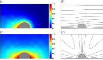Near $Pe\approx 30$, the growth rates of the higher-order modes are seen to outweigh the dipolar self-propulsion mode, and this could be a reason for the qualitative change in the dynamics of the particle from the swimming to the stirring regime. The transition may also be examined by a comparison of the concentration profile of the solute cloud, and the streamlines of the flow profile, at two different values of $Pe$, as illustrated in figure 2. The solute distribution around the autophoretic particle is fore–aft asymmetric at $Pe=20$, but is nearly fore–aft symmetric at $Pe=30$ with a maximum concentration at the front and rear stagnation points. Furthermore, the streamlines in figure 2(d) indicate a recirculation of the fluid around the autophoretic particle, where fluid is brought in along the polar axis and expelled at the equator. This flow pattern is consistent with the dominance of a quadrupolar disturbance to concentration profile. This region of parameter space $27\leq Pe\leq 50$ is therefore analogous to the symmetric extensile pumping regime identified by Morozov & Michelin (Reference Morozov and Michelin2019), wherein the activity of the particle results in the stirring of the fluid around it, without resulting in its self-propulsion.

Figure 2.

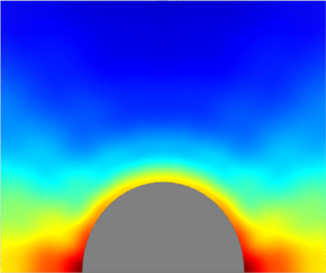
Steady-state concentration profile and streamlines of the flow around the autophoretic particle at $Pe=20$ (a,b) and (b) $Pe=30$ (c,d). The flow and concentration fields are symmetric about the horizontal axis; therefore, only half the particle is shown. The colour bar indicates the value of the solute concentration $c$.

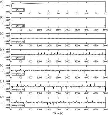
In figure 3, the instantaneous self-propulsion speed of the autophoretic particle is plotted as a function of time for various values of $Pe$. The swimming speed in the steady regime, as seen from figure 3(a), settles to a constant value of ${O}(10^{-1})$ following an initial transient, while that in the stirring regime (shown in figure 3(b)) is orders of magnitude lower. Beyond $Pe=51$, an onset of oscillations in the swimming speed is observed. While these oscillations are transient and vanish at long times for $Pe=52$, they become persistent at $Pe=53$, as seen from figures 3(c) and 3(d), respectively. With a further increase in $Pe$, the particle begins to move back and forth along the $z$-axis, the time scale for the reversal in self-propulsion direction decreases and the magnitude of the instantaneous self-propulsion speed increases, as seen from figures 3(e)–3(g). 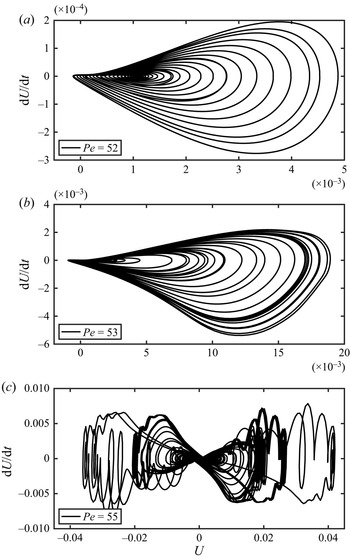The region $Pe\geq 55$ may be termed as the chaotic regime, characterized by short bursts of self-propulsion in arbitrary directions (along the $\pm z$-axis) and sharp changes in both the magnitude and direction of the self-propulsion speed. This transition to chaos occurs through a period-doubling cascade, as illustrated through the phase-plane diagram $(\textrm {d} U/\textrm {d} t,U)$ in figure 4. The pattern of closed loops in figures 4(a) and 4(b), corresponding to $Pe=52$ and $Pe=53$, respectively, is qualitatively similar to that reported by Hu et al. (Reference Hu, Lin, Rafai and Misbah2022), who also observe a period-doubling route to chaos. As the Péclet number is increased to $Pe=55$ (figure 4c) the trajectory resembles the familiar butterfly-shaped pattern observed in chaotic systems (Strogatz Reference Strogatz2015).

Figure 3.

Time evolution of the self-propulsion speed at (a) $Pe=10$, (b) $Pe=40$, (c) $Pe=52$, (d) $Pe=53$, (e) $Pe=55$, ( f) $Pe=58$, (g) $Pe=60$.

Figure 4.

Phase-plane diagram at (a) $Pe=52$, (b) $Pe=53$ and (c) $Pe=55$.

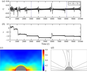
The dynamics in the chaotic regime is explored further by considering a representative case of $Pe=75$. The time series of instantaneous self-propulsion speed at $Pe=75$ is shown in figure 5(a). Following an initial transient that lasts till $t\approx 3000$, the velocity settles into a characteristic pattern, with intermittent bursts of chaos that interrupt nearly regular oscillations of slowly varying amplitude (Bérge, Pomeau & Vidal Reference Bérge, Pomeau and Vidal1984). The instantaneous position of the particle along the $z-$axis, evaluated using (3.6), is plotted in figure 5(b) as a function of time. After a transient period, the particle is seen to oscillate about a mean position of $z=-1$. The time-averaged concentration profile and streamlines of flow around the autophoretic particle, evaluated in the window $t\in (3000,8000)$, are plotted in figures 5(c) and 5(d), respectively. The concentration map is largely fore–aft symmetric, and this is consistent with the limited (net) mobility of the particle seen in (b). The pattern of the streamlines is qualitatively similar to that observed in the stirring regime (cf. figure 2d). 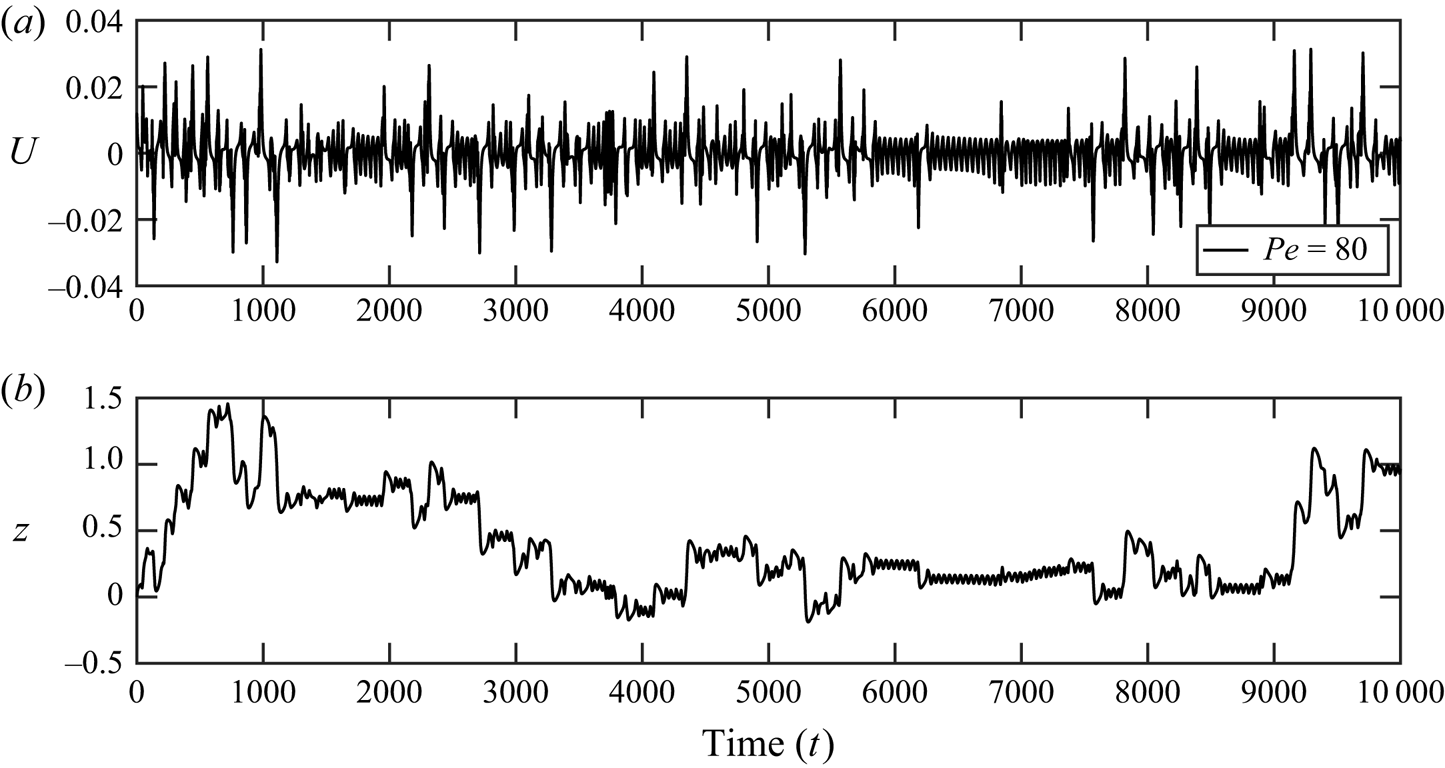A similar behaviour is observed at $Pe=80$, following an initial transient period that lasts till $t\approx 1500$. The intermittent bursts of chaos are more frequent, however, as observed in figure 6(a). Due to the more frequent injections of this ‘turbulent’ motion, the particle travels a larger distance than at $Pe=75$, as seen from figure 6(b). While the velocity and displacement time series of the autophoretic particle in the chaotic regime vary markedly depending upon the Péclet number, an analysis of the particle's MSD and VAC reveals certain unifying features, as discussed below.

Figure 5.

Time evolution of (a) the self-propulsion speed, and (b) displacement along $z-$ axis, for an autophoretic particle at $Pe=75$. The complete simulation output in the window $t\in (3000,8000)$ is saved at intervals of fifty dimensionless time units. The time-averaged concentration profile and streamlines of the flow around the autophoretic particle in this window are shown in (c) and (d), respectively.

Figure 6.

Time evolution of (a) the self-propulsion speed, and (b) displacement along $z-$ axis, for an autophoretic particle at $Pe=80$.

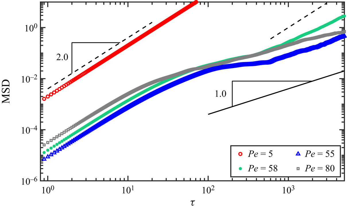
In figure 7, the MSD of the particle is plotted as a function of the lag time for a range of Péclet numbers. At $Pe=5$, corresponding to steady self-propulsion, the MSD grows as $\sim \tau ^2$, since the particle moves rectilinearly at a constant speed. Péclet numbers in the range $27\leq Pe <50$ are not examined since the particle is practically stationary, with only the fluid around it undergoing symmetric pumping, or stirring. At $Pe=55$ and $Pe=58$, the MSD grows quadratically with the lag time at early times, followed by a region of slower growth, before appearing to tend toward a long-time ballistic regime. This evolution may be qualitatively compared with the findings by Hu et al. (Reference Hu, Lin, Rafai and Misbah2022), who observed for $Pe=54$ that the MSD has an early-time and late-time ballistic regime. At $Pe=80$, however, only an early-time ballistic motion is observed, followed by a transition to what more closely resembles a diffusive regime (MSD $\sim \tau$). While such a trend is not observed in axisymmetric simulations of Hu et al. (Reference Hu, Lin, Rafai and Misbah2022), who do not report computational results for $Pe>60$, it is similar to the transition to diffusive motion observed their 3-D simulations, albeit at lower values of the Péclet number ($Pe\approx 24.5$). The different MSD behaviours observed for $Pe=55$ and $Pe=80$ can be interpreted in terms of the differences in the velocity time series at these two Péclet numbers: the time series at $Pe=55$ (figure 3e) is within the window of period doubling identified by Hu et al. (Reference Hu, Lin, Rafai and Misbah2022), whereas that for $Pe=80$ contains bursts of intermittent chaos (figure 6a). Thus, we conjecture that the long-time diffusive motion of an autophoretic particle, whether constrained to axisymmetric motion or free to move in three dimensions, is due to intermittency in its chaotic dynamics.

Figure 7.

Mean square displacement of an autophoretic particle at various Péclet numbers. Broken lines indicate a slope of $2$, while solid line has a slope of $1$.

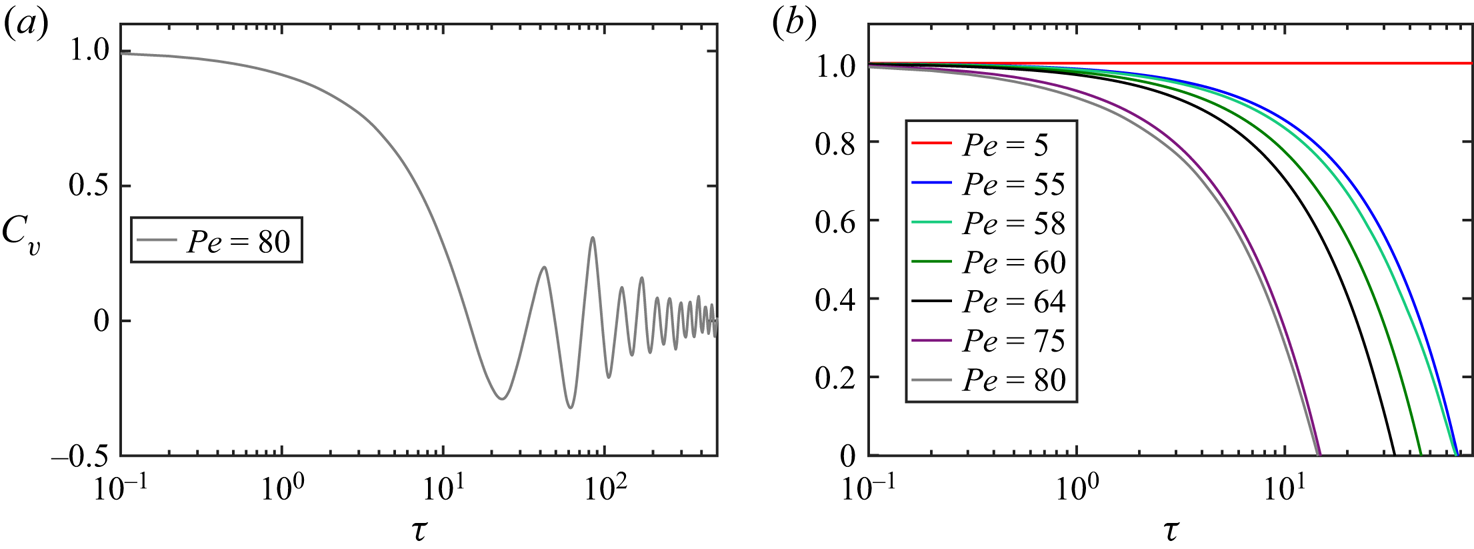
In figure 8(a), the VAC function for an autophoretic particle with $Pe=80$ is plotted as a function of time. Rapid changes in the direction of self-propulsion result in a decorrelation of the signal, which crosses zero at $\tau \approx 15$. This is followed by the appearance of negative dips and oscillations in the VAC: these features have also been observed experimentally by Suda et al. (Reference Suda, Suda, Ohmura and Ichikawa2021) and Hokmabad et al. (Reference Hokmabad, Dey, Jalaal, Mohanty, Almukambetova, Baldwin, Lohse and Maass2021), as discussed below in detail. The variation in the VAC with $Pe$ is illustrated in figure 8(b), where the data for $Pe\geq 55$ have been shown only until the first instance of their crossing zero, for clarity. A decrease in the Péclet number from $Pe=80$ results in less rapid changes in the particle motion, which is reflected in the longer time required for the velocity to decorrelate. Finally, at $Pe=5$, the VAC is constant in time, indicating a complete correlation in the velocity, due to the persistent unidirectional translation of the particle. Such a decrease in the correlation time with an increase in $Pe$ has also been reported by Chen et al. (Reference Chen, Chong, Liu, Verzicco and Lohse2021), who performed 3-D simulations of a phoretic particle using the immersed boundary method. That study, however, does not report a zero crossing in the VAC for the range of lag times investigated.

Figure 8.

Velocity autocorrelation of an active particle (a) at $Pe=80$, and (b) over a range of Péclet numbers.

Experiments on water droplets in a mixture of oil and surfactant (Suda et al. Reference Suda, Suda, Ohmura and Ichikawa2021), as well as oil droplets in an aqueous surfactant solution (Hokmabad et al. Reference Hokmabad, Dey, Jalaal, Mohanty, Almukambetova, Baldwin, Lohse and Maass2021), have both shown that the decorrelation in the droplet velocity is faster at larger values of $Pe$, in qualitative agreement with the trends in figure 8(b). In these experiments, the droplets undergo self-propulsion due to a Marangoni stress imbalance at the interface, driven by a reaction between the droplet contents and the surfactant, resulting in the generation of oil-filled micelles. The active droplets undergo a transition from ballistic motion to anomalous diffusion with an increase in the Péclet number (Hokmabad et al. Reference Hokmabad, Dey, Jalaal, Mohanty, Almukambetova, Baldwin, Lohse and Maass2021), which is accompanied by a faster decay in the VAC. The droplets are found to avoid the chemical trail that they generate, and undergo a 2-D self-avoiding walk, with MSD $\sim \tau ^{3/2}$. This route for trail avoidance is not possible for the axisymmetric model considered here, and is a major point of distinction from the 2-D experiments discussed above. This could also potentially be the reason for the slower growth in the MSD at long times, leading to a near-diffusive regime observed at $Pe=80$.

5. Forced autophoretic particle

Saha et al. (Reference Saha, Yariv and Schnitzer2021) have derived asymptotic approximations to the motion of an autophoretic particle subjected to a weak external force ($\epsilon \ll 1$). Specifically, they have obtained ‘global’ and a ‘local’ approximations to this problem. In the global approximation an $O(\epsilon )$ perturbation is constructed to the trivial solution of an unforced particle, where the solute concentration is isotropic and there is no flow. This leads to the prediction $U\sim \epsilon (8-AMPe)/[2(4-AMPe)]$ as $\epsilon \to 0$. Thus, increasing $Pe$ for $AM=-1$, where the trivial solution is stable, leads to a reduction in the speed of particle translation due to diffusio-osmotic flow around the particle. 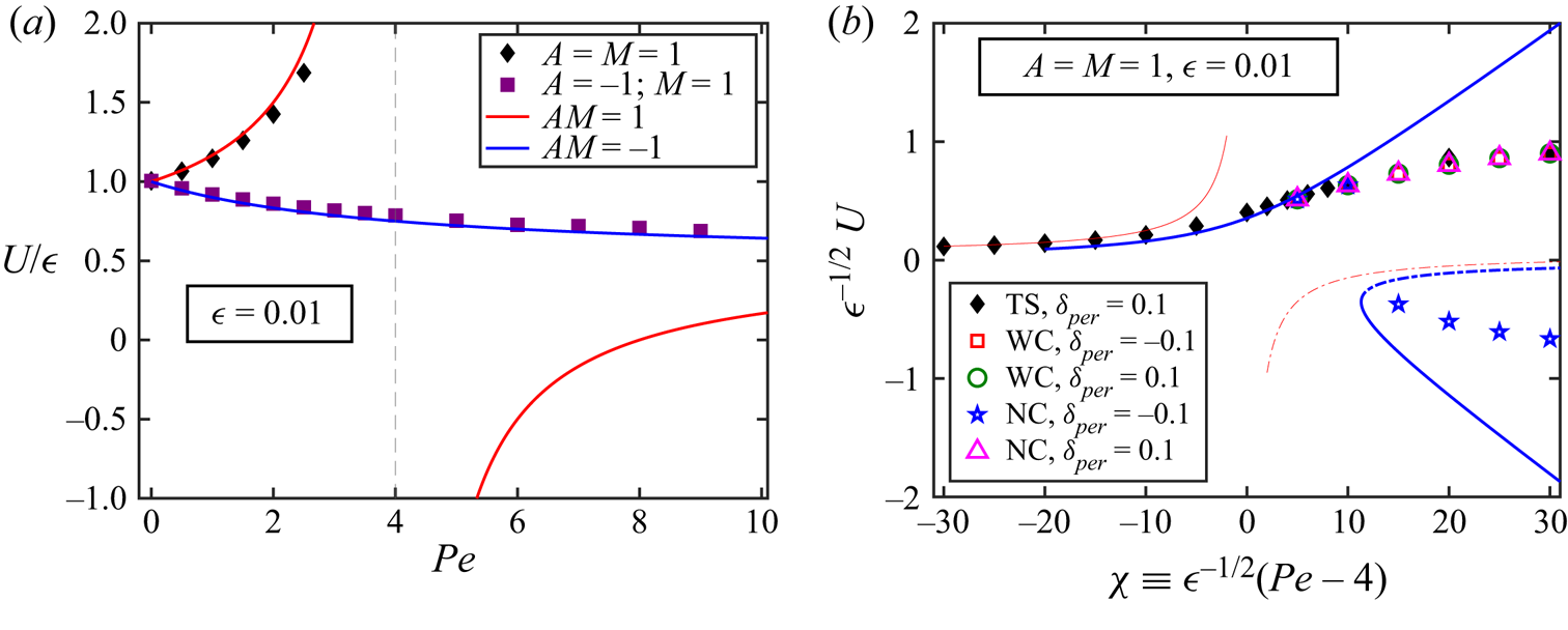The case of $AM=1$ is more interesting: here, the instability of the unforced problem at $Pe=4$ is manifested as a divergence in the global approximation at this value of $Pe$. A comparison of their global prediction against our numerical solution is shown in figure 9(a). For $AM=1$ the numerical result matches well with the approximate global solution at small values of $Pe$. For $AM=-1$ the global approximation and the numerical results agree over a larger range of the Péclet number.

Figure 9.

Scaled self-propulsion speed of a forced autophoretic particle with $\epsilon =0.01$. Symbols are numerical results, and in (a) lines are analytical predictions from the global analysis of Saha et al. (Reference Saha, Yariv and Schnitzer2021); in (b) thick lines denote solutions from their local analysis, and thin lines represent the global solution. Solid lines denote the stable solution branch, while the broken lines represent the unstable branch. Filled symbols indicate solutions obtained using the transient solver (TS), while hollow symbols denote results obtained using the iterative solver. Results obtained with and without a continuation scheme have been denoted by the abbreviations ‘WC’ and ‘NC’ respectively.

Saha et al. (Reference Saha, Yariv and Schnitzer2021) have also derived a local approximation for the particle translation speed, valid in the vicinity of the bifurcation point of the unforced problem, $Pe=4$. More specifically, this approximation is valid when the variable $\chi \equiv \epsilon ^{-1/2}(\mathrm {Pe}-4)=O(1)$ as $Pe\to 4$; that is, $\chi$ represents the appropriate deviation from the bifurcation point. The results for the particle speed are given in (8.1) to (8.3) of Saha et al. (Reference Saha, Yariv and Schnitzer2021) and not repeated here for brevity. In summary, the speed is of $O(\epsilon ^{-1/2})$ near the bifurcation point, and there are two stable solutions branches: one corresponds to $U>0$ and smoothly matches to the global approximation as $\chi \to \infty$; and the other corresponds to $U<0$ and only exists for $\chi >8\sqrt {2}$. There is also an unstable branch with $U<0$ for $\chi >8\sqrt {2}$. This is the classic scenario of an imperfect (singular) pitchfork bifurcation. The stable branch with $U<0$ suggests that steady propulsion is possible in a direction anti-parallel to the external force, which is remarkable. On this note, experiments on the sedimentation of active droplets in a semicylindrical glass container (Moerman Reference Moerman2019) show that, above a critical Péclet number, the droplets move transiently against the direction of the biasing force (i.e. gravity). We are not aware, however, of experiments in which an active particle/drop undergoes steady self-propulsion against the direction of the external force.

In figure 9(b), the particle speed for $AM=1$ computed from the present work, scaled by $\epsilon ^{-1/2}$, is compared against their local approximation. The agreement is good near the bifurcation point ($\chi =0$). Four different numerical scenarios are examined in figure 9(b) for the iterative solver corresponding to various choices of $\delta _{{per}}$ and whether or not a continuation scheme is applied, wherein the converged concentration field at a particular value of the Péclet number is used as the initial guess for the computation at the next higher value of $Pe$. At $\delta _{{per}}=0.1$, the numerical predictions of the iterative solver are identical, irrespective of whether continuation is employed. With $\delta _{{per}}=-0.1$, contrasting trends are observed: using a continuation scheme, the predictions agree with those obtained for the $\delta _{{per}}=0.1$ case. However, in the absence of continuation, a stable steady self-propulsion is observed in the direction opposite to the external forcing, for $\chi \geq 15$. Using the converged concentration field at these Péclet numbers as the initial condition for the transient solver, however, predicts a steady phoretic speed in the direction of the external forcing, i.e. a jump from the anti-parallel to parallel branches of the local approximation. Additionally, the results predicted by the transient solver for the range of $Pe$ examined in figure 9(b) are unaltered by the choice of $\delta _{{per}}$, or the use of a continuation scheme. These results only lead to motion with $U>0$.

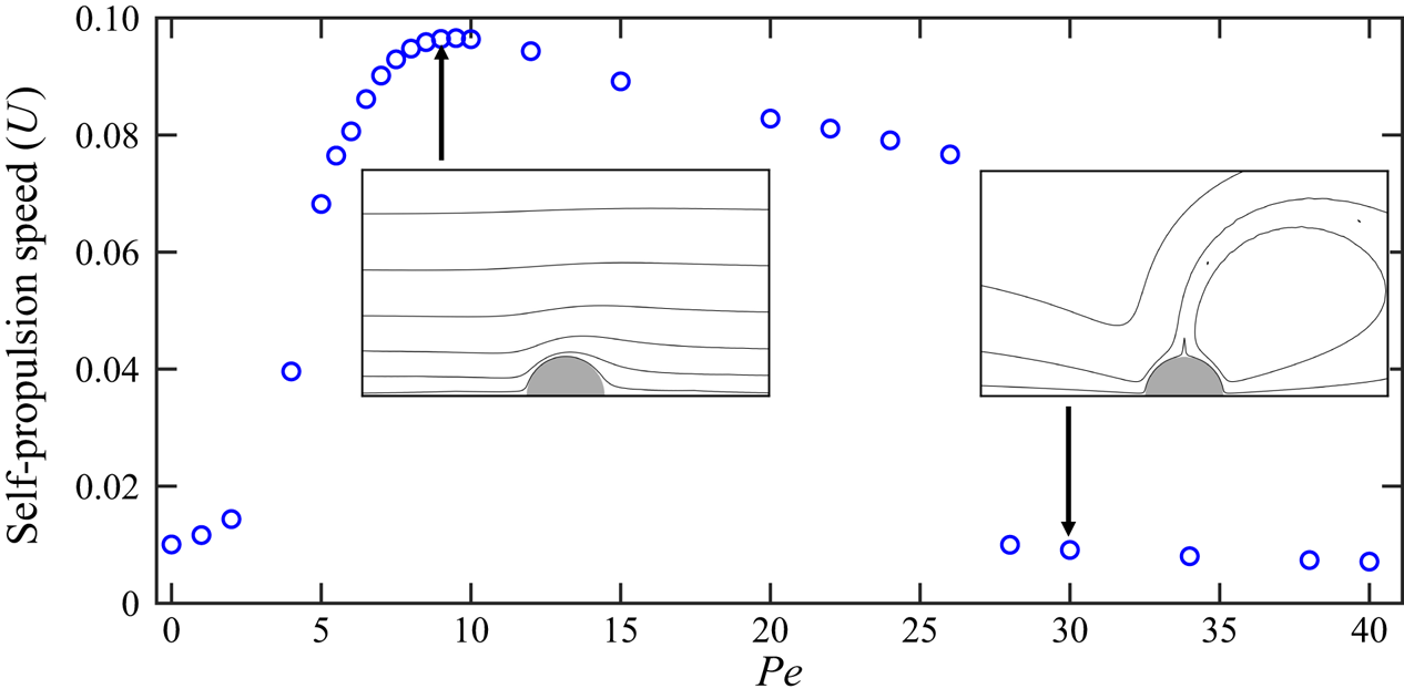
The variation of the steady self-propulsion speed for a particle with $AM=1$ and $\epsilon =0.01$ over a larger range of Péclet number is shown in figure 10. There is no quiescent regime for such a particle, and the self-propulsion speed increases with the Péclet number up to $Pe\approx 10$, before decreasing. At $Pe\approx 28$, an abrupt decrease in the self-propulsion speed is observed, which is accompanied by a recirculation region in front of the particle. This represents a perturbed form of the stirring regime observed for an unforced particle, where the fore–aft symmetry in the flow profile is due to the weak external force. 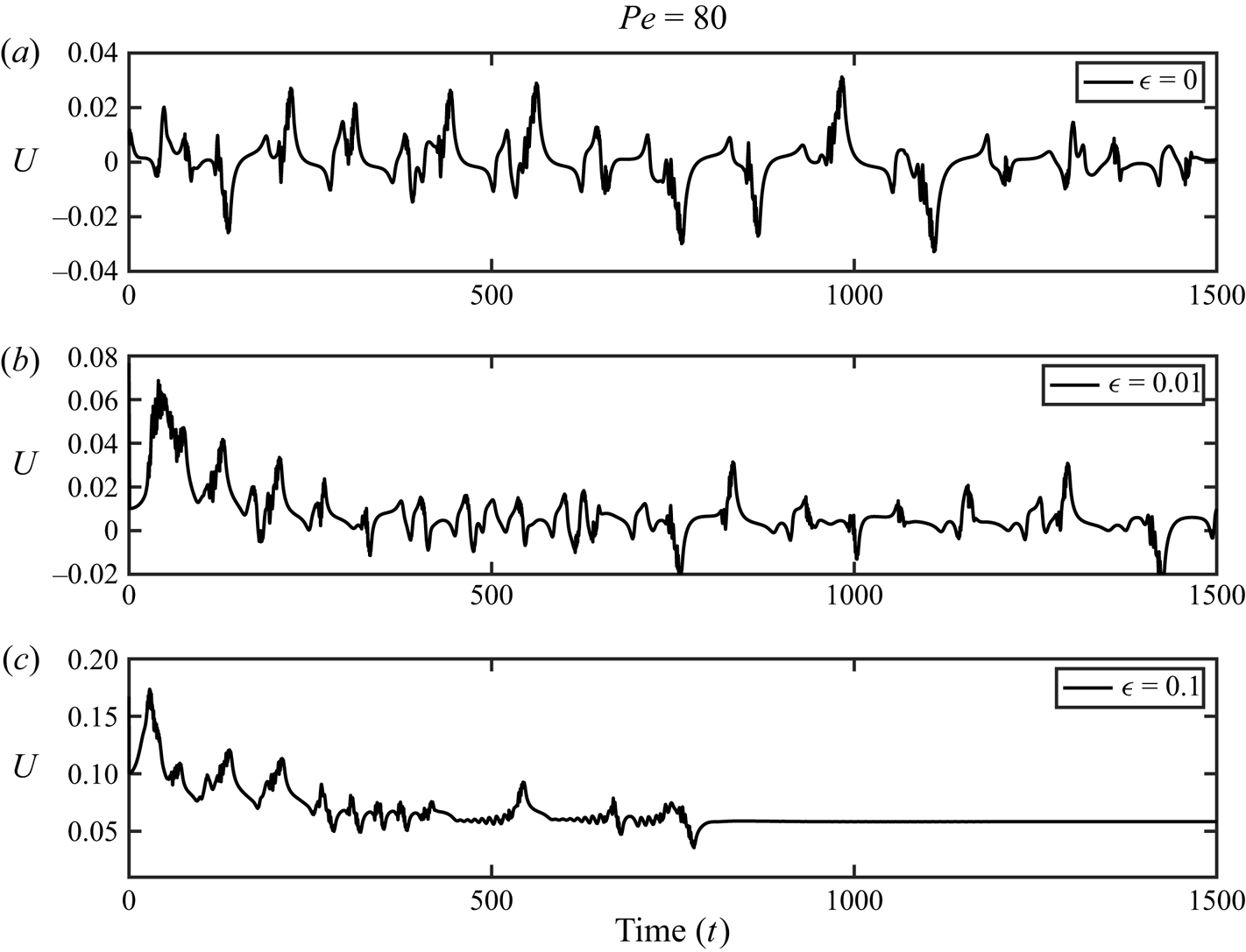The qualitative similarity of the particle speed variation with $Pe$ to that of an unforced particle suggests that chaotic dynamics should occur at sufficiently large $Pe$, and this is indeed the case. In figure 11, the effect of a steady force on the chaotic dynamics of an autophoretic particle is illustrated, at a representative value of $Pe=80$ for $\epsilon =0, 0.01$ and $0.1$. Increasing the value of $\epsilon$ quenches the chaos, as seen for $\epsilon =0.1$, where the particle attains a steady translation speed after an initial period of transient chaotic self-propulsion. However, at $\epsilon =0.01$ the magnitude of the external force is not sufficient to quench the chaos. Nonetheless, following a transient period that lasts till $t\approx 1000$, the time-averaged value of the self-propulsion speed is observed to increase commensurately, relative to the unforced case, with the magnitude of the external force.

Figure 10.

Translation speed of an autophoretic particle with $A=M=1$ and $\epsilon =0.01$. The insets show the streamlines of the flow around the particle at $Pe=9$ and $Pe=30$.

Figure 11.

Transient translation speed of an autophoretic particle with $Pe=80$ and (a) $\epsilon =0.0$, (b) $\epsilon =0.01$ and (c) $\epsilon =0.1$.

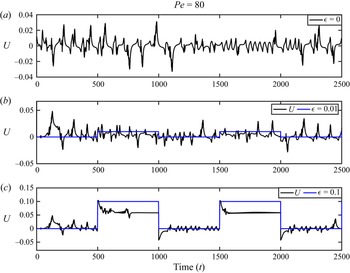
In figure 12, we demonstrate the effect of a time-dependent external force on the chaotic dynamics. The external force is varied between zero and a fixed value of $\epsilon$ over a time interval $t_{{box}}=500$. The difference in the average self-propulsion speed between adjacent blocks computed over the interval $t_{{box}}$ is $\approx \epsilon /2$ for both of the non-zero values of the dimensionless external force considered in figure 12. At $\epsilon =0.1$ the external force is of sufficient strength to eventually quench the chaotic dynamics during the time when the external force switched on. Thus, even a relatively weak external force can significantly alter the dynamics of an autophoretic particle within the chaotic regime. Our computations are axisymmetric, which restricts the particle motion to be along the direction of the external force. However, we expect our conclusions to hold qualitatively for unconstrained (i.e. three-dimensional) motion. For example, with reference to figure 12, a time-dependent external forcing could lead to transient alignment of the particle motion with the direction of the external force, whereas unconstrained chaotic motion occurs during times when the external force is switch off.

Figure 12.

Transient translation speed of an autophoretic particle with $Pe=80$ and (a) $\epsilon =0.0$, (b) $\epsilon =0.01$ and (c) $\epsilon =0.1$. (a) Corresponds to an unforced particle, while the time-dependent forcing has been indicated by blue lines in (b,c).