1 Introduction
Social scientists regularly confront situations that require some type of model selection. This may include selecting the shape of the relationship between an explanatory variable and an outcome. Or, as is the focus in this paper, it may involve “sparse modeling,” an estimation technique that zeroes out all but the most relevant of variables from hundreds or thousands of possible candidates. Earlier approaches to these situations, such as step-wise regression, have in recent years been replaced by new tools, including those provided by the growing machine learning literature.Footnote 1 Many of these tools use some form of “regularization” or “sparsity” where estimates can be shrunk or removed from the model according to a thresholding rule. As one applied example of variable selection, a subgroup analysis involves estimating which combinations of treatments are most (or least) efficacious, and for which observations (Berry Reference Berry1990). As experimental designs grow more complex (e.g., Hainmueller et al. Reference Hainmueller, Hopkins and Yamamoto2014), the number of candidate subgroup effects has grown as well. In turn, social scientists have grown increasingly interested in methods for uncovering subgroup effects (e.g. Grimmer et al., Reference Grimmer, Messing and Westwoodforthcoming; Imai and Ratkovic Reference Imai and Ratkovic2013; Green and Kern Reference Green and Kern2012), with some of these methods using regularization-based variable selection methods.
In this paper, we introduce LASSOplus,Footnote 2 a Bayesian method for variable selection in high-dimensional settings. LASSOplus offers two major statistical advances over existing Bayesian shrinkage and selection methods (Park and Casella Reference Park and Casella2008; Carvalho et al. Reference Carvalho, Polson and Scott2010; Armagan et al. Reference Armagan, Dunson and Lee2013; Leng et al. Reference Leng, Tran and Nott2014; Griffin and Brown Reference Griffin and Brown2012, Reference Griffin and Brown2010; Kang and Guo Reference Kang and Guo2009). First, LASSOplus is the first sparse Bayesian method for variable selection, whereby effects are simultaneously estimated and selected. Second, LASSOplus has been designed to possess desirable theoretical properties. We focus our theoretical attention on cases where the number of possible effects are either growing in or even greater than the sample size. LASSOplus has the Oracle Property described by Fan and Li (Reference Fan and Li2001), which means that it is asymptotically indistinguishable from a model fit only to covariates with an in-truth nonzero effect. It also satisfies an Oracle Inequality (Candes Reference Candes2006), so it achieves a prediction error of the same order as least squares fit to the true model. Third, LASSOplus returns approximate confidence intervals. As a Bayesian method, LASSOplus returns credible intervals, but previous methods have found that these credible intervals are more narrow than the confidence intervals (Kyung et al. Reference Kyung, Gill, Ghosh and Casella2010). For the researcher interested in confidence intervals, we return uncertainty intervals that are calibrated to achieve nominal coverage (Efron Reference Efron2015). Our goal is to produce a method useful to the applied researcher, so our implementation of LASSOplus includes extensions to several commonly encountered data structures and types. The software, which we make publicly available in the R programming language, handles binary and truncated outcomes, computes up to three-way random effects, and has both a full Markov Chain Monte Carlo implementation and a faster Expectation–Maximization implementation, a useful tool for practical modeling.
To illustrate the usefulness of LASSOplus, we apply the method to subgroup analysis. Existing subgroup analysis methods face several shortcomings. Frequentist tree-based methods identify subgroups, but they do not offer uncertainty estimates nor can they handle experiments with repeated observations (Loh et al. Reference Loh, Heb and Manc2015; Foster et al. Reference Foster, Taylor and Ruberg2011; Imai and Strauss Reference Imai and Strauss2011; Lipkovich et al. Reference Lipkovich, Dmitrienko, Denne and Enas2011; Su et al. Reference Su, Tsai, Wang, Nickerson and Li2009), but see Wager and Athey (Reference Wager and Athey2015). Frequentist variable selection methods also cannot handle repeated observations (Imai and Ratkovic Reference Imai and Ratkovic2013), and their methods for estimating confidence intervals perform poorly in our simulations (Minnier et al. Reference Minnier, Tian and Cai2011). Recent work has implemented ensemble or high-dimensional Bayesian methods (Berger et al. Reference Berger, Wang and Shen2015; Green and Kern Reference Green and Kern2012; Grimmer et al., Reference Grimmer, Messing and Westwoodforthcoming). These methods are powerful predictive tools, but they do not point-identify relevant subgroups. They work by fitting either a single black-box model or several different models, and subgroups are identified through an ex post, ad hoc search. The uncertainty estimates (if they are even available) are not guaranteed to have nominal coverage, and implementations of the machine learning methods do not accommodate repeated observations.
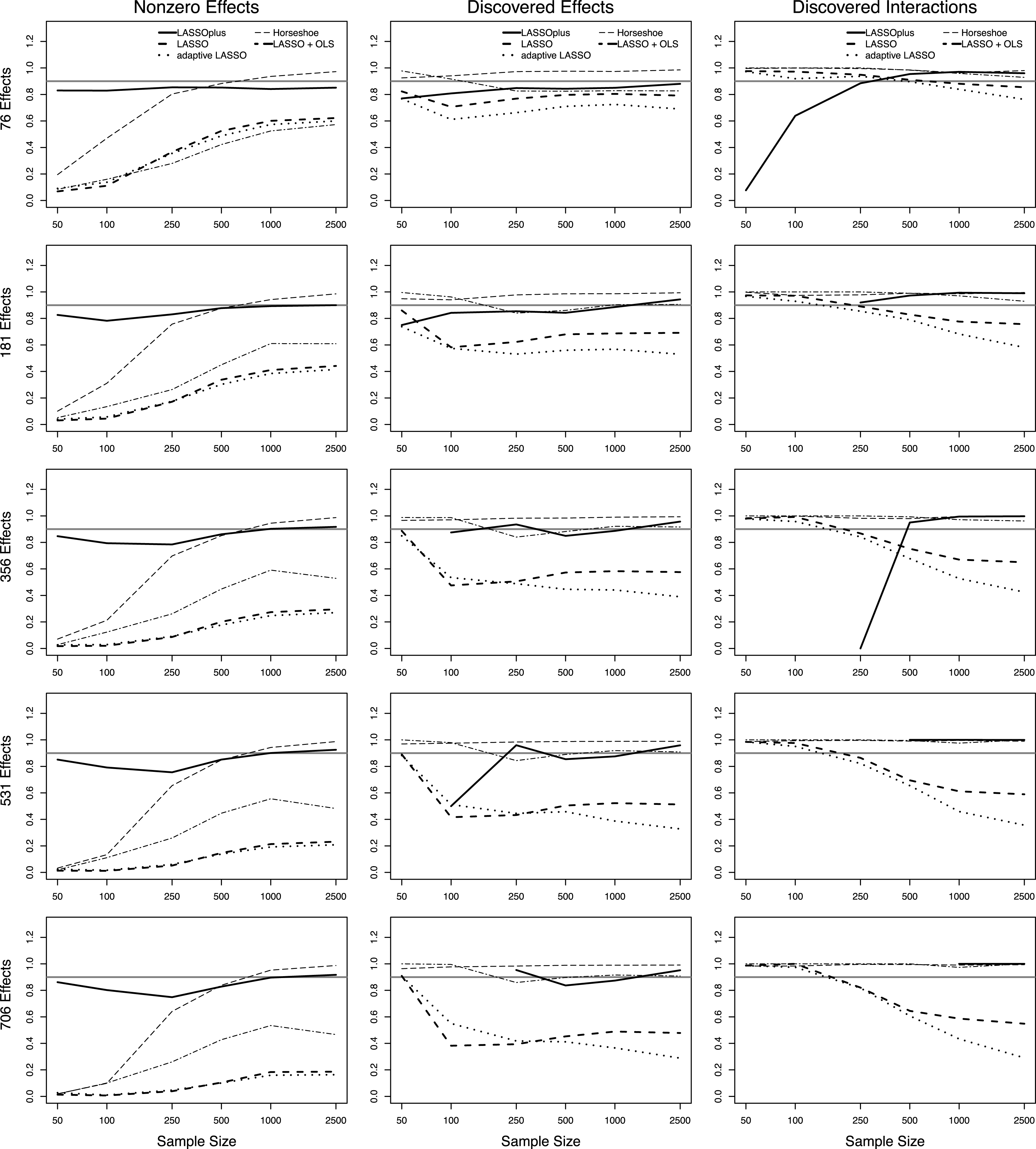
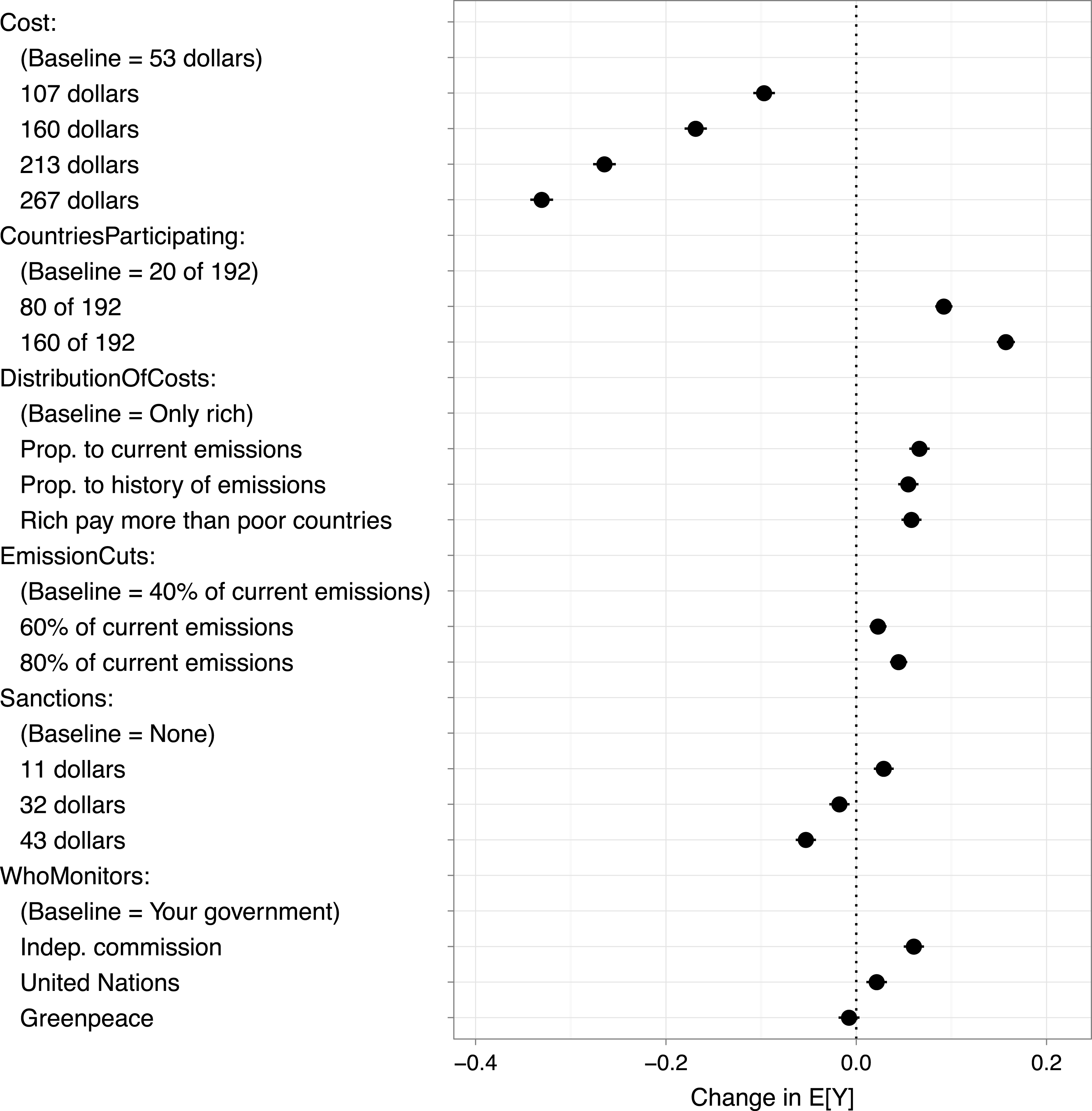
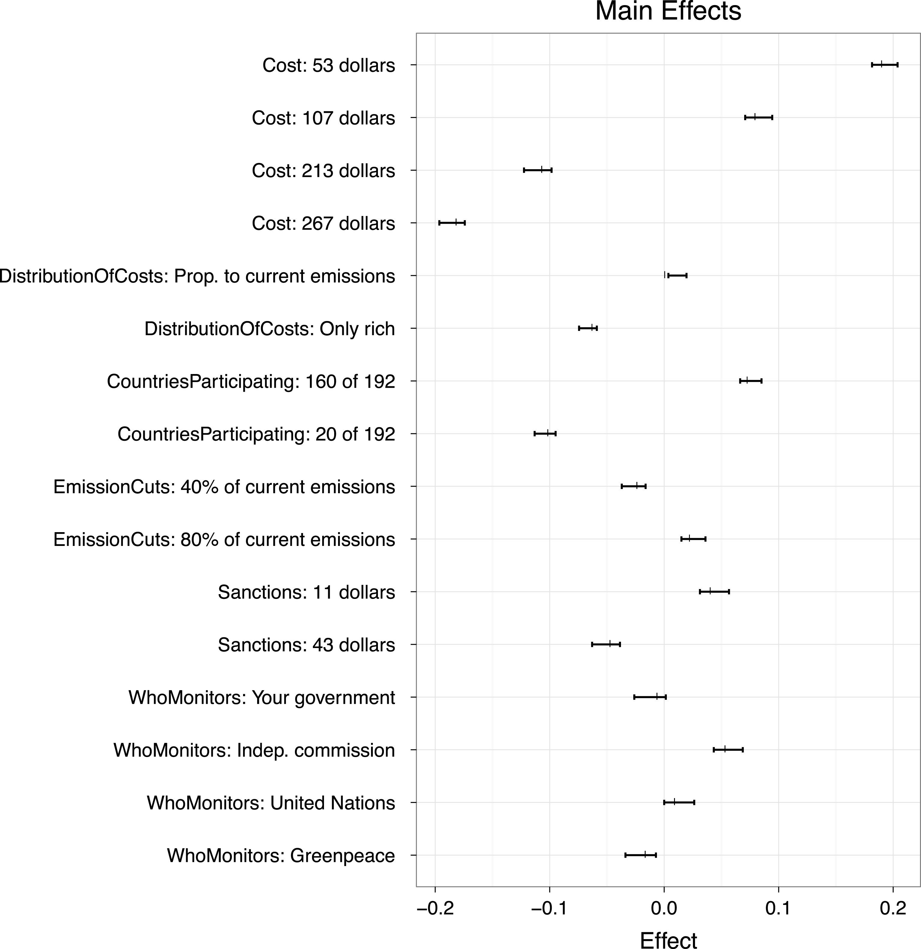
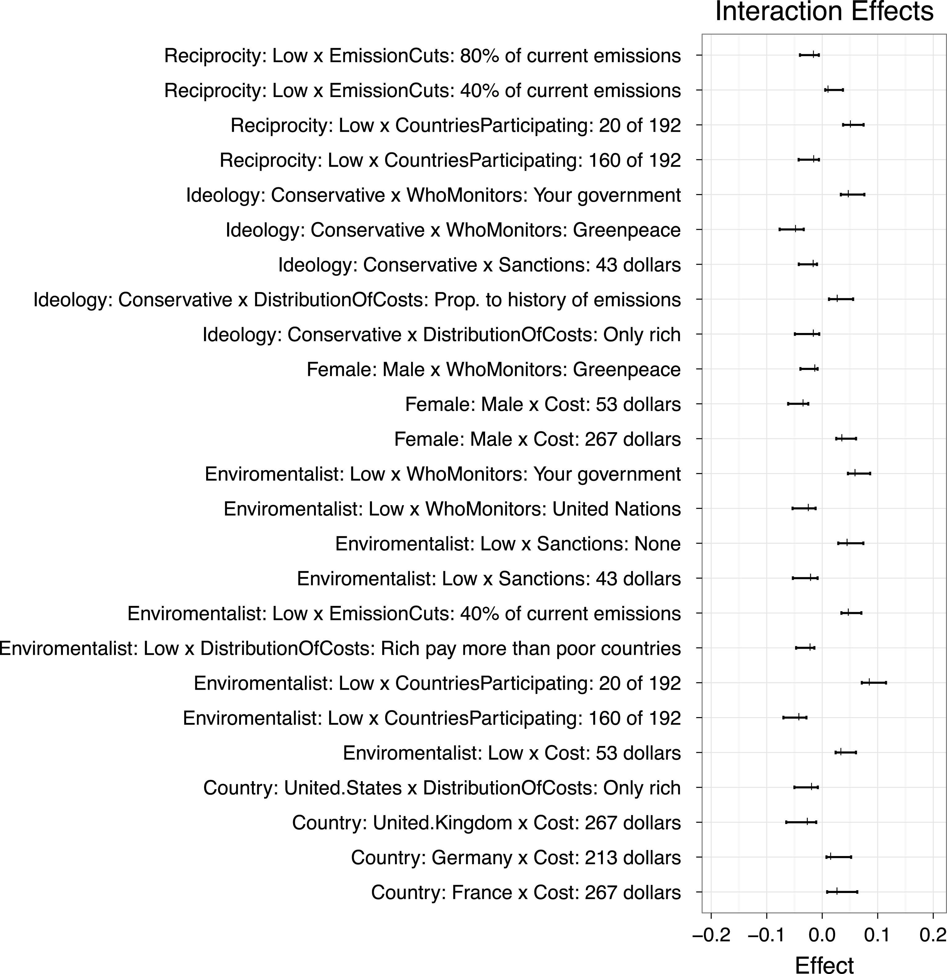
We present a simulation study that compares LASSOplus to other cutting edge methods. LASSOplus achieves a false discovery rate lower than that of several existing methods, often dramatically so. The method remains reasonably powerful, and its approximate confidence intervals achieve nominal or near-nominal coverage. We also apply the method to a recent conjoint experiment by Bechtel and Scheve (Reference Bechtel and Scheve2013) in which the authors estimate the effects of different features of an international climate change agreement on voter support. The original authors conduct an extensive set of subgroup analyses by running a regression after repeatedly subsetting their data. Our method recovers many of the same effects, avoids the arbitrary nature of subsetting, is implemented in one line of code, and returns uncertainty estimates on each effect that take into account the fact that individuals respond to multiple versions of the experiment.
The structure of the paper reflects our three main goals. First, in Section 2, we introduce readers to core concepts and existing methods for LASSO-based variable selection. Second, Sections 3 and 4 introduce the LASSOplus and state its statistical properties, while Section 5 discusses relevant issues arising during the application and interpretation of the method for subgroup analysis. Third, we illustrate the application of LASSOplus in Section 6 by comparing it to earlier methods using an extensive Monte Carlo simulation study and in Section 7 we apply the method to the case of subgroup analysis by analyzing the data in Bechtel and Scheve (Reference Bechtel and Scheve2013). We show how LASSOplus recovers many of the original authors’ subgroup results while making minimal modeling decisions. Section 8 concludes with key contributions and discusses future research opportunities.
2 Variable Selection and Shrinkage
Given observed outcome
 $Y_{i}$
and vector of
 $K$
observed covariates
 $X_{i}$
on observation
 $i\in \{1,2,\ldots ,N\}$
, researchers will commonly turn to the linear model to connect the two, as
 $$\begin{eqnarray}\displaystyle Y_{i}=X_{i}^{\top }\unicode[STIX]{x1D6FD}^{o}+\unicode[STIX]{x1D716}_{i} & & \displaystyle\end{eqnarray}$$
where
 $\unicode[STIX]{x1D6FD}^{o}$
is the population-level vector of parameters associated with each covariate and
 $\unicode[STIX]{x1D716}_{i}$
is the error term, assumed mean zero and equivariant. We will also assume that
 $Y_{i}$
is mean zero, so
 $\sum _{i=1}^{N}Y_{i}=0$
and that each element of
 $X_{i}$
is scaled to be mean zero and have a sample standard deviation one, so
 $\sum _{i=1}^{N}X_{ik}=0$
and
 $\sum _{i=1}^{N}X_{ik}^{2}=N-1$
.
Social scientists are well trained on how to handle the case where
 $N\gg K$
. Valid inference can be conducted using the familiar
 $t$
- or
 $z$
-statistics,
 $p$
-values, and confidence intervals. We work here on a different problem: how to fit this model when there are hundreds or thousands of elements in
 $X_{i}$
and return the handful that best explain the outcome. When
 $K$
is large, least squares estimates are unstable, and when
 $K>N$
, a unique estimate does not even exist.
This setting may at first seem unfamiliar or esoteric, but it is not. Once we consider
 $X_{i}$
as consisting of all main effects and two- and three-way interaction terms, even a modest number of variables can produce a large number of covariates (e.g., Gillen et al.
Reference Gillen, Montero, Moon and Shum2016). In our application below, we consider data from a conjoint experiment, where main effects plus treatment
 $\times$
covariate interactions generated 215 possible subgroup effects. Rather than present three or four pages of output from a regression table, we implement LASSOplus, producing 41 nonzero effects. Thus LASSOplus opens the door to allow for models that are saturated with interaction terms, while still returning efficient estimates that can add nuance to the underlying theory.
LASSOplus is an example of a “sparse model.” Sparse modeling involves fitting a model that zeroes out all but some small subset of
 $\widehat{\unicode[STIX]{x1D6FD}}$
. The literature on sparse modeling is large and diverse, so we first introduce several of the key concepts, contributions, and insights. For ease of exposition, we focus on variable selection in the single-parameter case, where
 $X_{i}$
is simply a scalar and the issue at hand is whether or not to set the estimate of
 $\unicode[STIX]{x1D6FD}^{o}$
to zero. After a brief survey of sparse modeling methods we turn to a description and evaluation of LASSOplus.
2.1 Standard practice: variable selection with one covariate
For this section, we assume an outcome
 $Y_{i}$
and single covariate,
 $X_{i}$
, both scaled as described above. We are going to consider variable selection in this simplified setting, with model
 $$\begin{eqnarray}\displaystyle Y_{i}=X_{i}\unicode[STIX]{x1D6FD}^{o}+\unicode[STIX]{x1D716}_{i} & & \displaystyle\end{eqnarray}$$
where the goal is how to decide whether or not to zero out
 $\widehat{\unicode[STIX]{x1D6FD}}$
. We focus on this simplified setting because it provides analytic results not available in the multivariate setting, and we use these results to convey the basic intuitions of variable selection. Later we return to the multivariate setting.
With a single covariate, variable selection is normally done in two stages: first, the effect is estimated and then some
 $p$
-value or
 $t$
-statistic threshold for statistical significance is used to determine whether the effect can be differentiated from zero. A standard estimate for
 $\unicode[STIX]{x1D6FD}^{o}$
is the least squares estimate,
 $$\begin{eqnarray}\displaystyle \widehat{\unicode[STIX]{x1D6FD}}^{LS} & = & \displaystyle \mathop{\text{argmin}}_{\widetilde{\unicode[STIX]{x1D6FD}}}\frac{1}{2}\mathop{\sum }_{i=1}^{N}(Y_{i}-X_{i}\widetilde{\unicode[STIX]{x1D6FD}})^{2}\end{eqnarray}$$
 $$\begin{eqnarray}\displaystyle & = & \displaystyle \frac{\mathop{\sum }_{i=1}^{N}Y_{i}X_{i}}{\mathop{\sum }_{i=1}^{N}X_{i}^{2}}=\frac{\mathop{\sum }_{i=1}^{N}Y_{i}X_{i}}{N-1}\end{eqnarray}$$
which gives a point estimate. The point estimate is then compared to its standard error,
 $\widehat{\unicode[STIX]{x1D70E}}_{\widehat{\unicode[STIX]{x1D6FD}}}:$
 $$\begin{eqnarray}\displaystyle \widehat{\unicode[STIX]{x1D70E}}_{\widehat{\unicode[STIX]{x1D6FD}}}=\frac{\widehat{\unicode[STIX]{x1D70E}}_{\unicode[STIX]{x1D716}}}{\sqrt{N-1}};\quad \widehat{\unicode[STIX]{x1D70E}}_{\unicode[STIX]{x1D716}}=\sqrt{\frac{\mathop{\sum }_{i=1}^{N}(Y_{i}-X_{i}\widehat{\unicode[STIX]{x1D6FD}}^{LS})^{2}}{N-2}}. & & \displaystyle\end{eqnarray}$$
If the
 $t$
-statistic is larger in magnitude than some critical value, normally 1.96, the effect is considered statistically significant. In this framework, estimation and selection occur in two separate steps. Estimation and selection cannot, in fact, be simultaneous: the least squares estimate is never zero, outside of pathological cases.
2.2 LASSO with a single covariate
Next we introduce the LASSO of Tibshirani (Reference Tibshirani1996) in the case with a single covariate. LASSO is an acronym for Least Absolute Shrinkage and Selection Operator. In the one-parameter case, the LASSO estimator is the solution to
 $$\begin{eqnarray}\displaystyle \widehat{\unicode[STIX]{x1D6FD}}^{L}=\mathop{\text{argmin}}_{\widetilde{\unicode[STIX]{x1D6FD}}}\frac{1}{2}\mathop{\sum }_{i=1}^{N}(Y_{i}-X_{i}\widetilde{\unicode[STIX]{x1D6FD}})^{2}+\unicode[STIX]{x1D706}|\widetilde{\unicode[STIX]{x1D6FD}}|. & & \displaystyle\end{eqnarray}$$
The first term in this objective function is the residual sum of a squares. The second term has two components: the tuning parameter
 $\unicode[STIX]{x1D706}$
, indexed by sample size, and the penalty term
 $|\widetilde{\unicode[STIX]{x1D6FD}}|$
. The least absolute component references the structure of the penalty,
 $\unicode[STIX]{x1D706}|\widetilde{\unicode[STIX]{x1D6FD}}|$
.
Denote the sign of the least squares estimate as
 $\widehat{s}^{L}=\text{sgn}(\widehat{\unicode[STIX]{x1D6FD}}^{LS})\in \{-1,1\}$
. With one parameter, the LASSO estimate is (Tibshirani Reference Tibshirani1996, Section 2.2)
 $$\begin{eqnarray}\displaystyle \widehat{\unicode[STIX]{x1D6FD}}^{L}=\left(\widehat{\unicode[STIX]{x1D6FD}}^{LS}-\widehat{s}^{L}\frac{\unicode[STIX]{x1D706}}{N-1}\right)\mathbf{1}\left(|\widehat{\unicode[STIX]{x1D6FD}}^{LS}|>\frac{\unicode[STIX]{x1D706}}{N-1}\right). & & \displaystyle\end{eqnarray}$$
The first part of Equation (7) illustrates the shrinkage: the estimate is the least squares estimate biased toward zero by
 $\unicode[STIX]{x1D706}/(N-1)$
. The second part of Equation (7) illustrates the selection component. If
 $\widehat{\unicode[STIX]{x1D6FD}}^{LS}$
is less than
 $\unicode[STIX]{x1D706}/(N-1)$
in magnitude, then the LASSO estimate is simply zero.
Equation (7) reveals three shortcomings of LASSO estimation. First,
 $\unicode[STIX]{x1D706}_{}$
must be estimated from the data. Researchers commonly turn to an AIC or BIC criterion or to cross-validation to select this tuning parameter. Unfortunately, these three methods may give quite different results, with little theoretical guidance to choose among them. Second, both large effects and small effects are biased toward zero by the same amount,
 $\unicode[STIX]{x1D706}/(N-1)$
. A more accurate estimator would shrink smaller effects but leave larger effects untouched. The third problem arises due to competing demands on
 $\unicode[STIX]{x1D706}/(N-1)$
. In the left side of the equation, it is a bias term. As such, we want it to go to zero quickly. In the right side of the equation, though, we see that if
 $\unicode[STIX]{x1D706}/(N-1)$
goes to zero too quickly, then we will end up not zeroing out any effects. As we show in Appendix A,Footnote
3
no LASSO model indexed by a single
 $\unicode[STIX]{x1D706}$
can produce estimates that are sparse, consistent, and asymptotically normal. The LASSOplus method proposed in this paper helps to resolve all three issues.
2.3 Single covariate adaptive LASSO
Zou (Reference Zou2006) introduced the adaptive LASSO, which extends the LASSO by including parameter-specific weights that cause differential shrinkage (see also Kenkel and Signorino Reference Kenkel and Signorino2012). These weights serve to shrink larger effects less than smaller effects. The adaptive LASSO is a two-stage estimator. In the first stage, weights that are inversely related to
 $\unicode[STIX]{x1D6FD}$
are constructed. In the second stage, these weights are used to weigh a LASSO problem. The weights are constructed as
 $$\begin{eqnarray}\displaystyle \widehat{w}=1/|\widehat{\unicode[STIX]{x1D6FD}}^{1}|^{\unicode[STIX]{x1D6FE}} & & \displaystyle\end{eqnarray}$$
where
 $\widehat{\unicode[STIX]{x1D6FD}}^{1}$
is a first-stage, root-N consistent estimate of
 $\unicode[STIX]{x1D6FD}^{o}$
and
 $\unicode[STIX]{x1D6FE}>0$
. With these weights, the estimator becomes
 $$\begin{eqnarray}\displaystyle \widehat{\unicode[STIX]{x1D6FD}}^{L}(\unicode[STIX]{x1D706})=\mathop{\text{argmin}}_{\widetilde{\unicode[STIX]{x1D6FD}}}\frac{1}{2}\mathop{\sum }_{i=1}^{N}(Y_{i}-X_{i}\widetilde{\unicode[STIX]{x1D6FD}})^{2}+\unicode[STIX]{x1D706}\widehat{w}|\widetilde{\unicode[STIX]{x1D6FD}}|. & & \displaystyle\end{eqnarray}$$
In this setting, the univariate adaptive LASSO estimator is
 $$\begin{eqnarray}\displaystyle \widehat{\unicode[STIX]{x1D6FD}}^{aL}(\unicode[STIX]{x1D706},w)=\left(\widehat{\unicode[STIX]{x1D6FD}}^{LS}-s\frac{w\unicode[STIX]{x1D706}}{N-1}\right)\mathbf{1}\left(|\widehat{\unicode[STIX]{x1D6FD}}^{LS}|>\frac{w\unicode[STIX]{x1D706}}{N-1}\right). & & \displaystyle\end{eqnarray}$$
For a fixed value of
 $\unicode[STIX]{x1D706}$
, the adaptive LASSO estimator has a lower bias for larger effects than smaller ones. With one effect, the adjustment is trivial, but with hundreds of possible effects, the gains from differential shrinkage can be substantial.
Several problems emerge with adaptive LASSO estimation. The first is that any number of methods can return a root-N consistent estimate of
 $\unicode[STIX]{x1D6FD}$
: least squares, ridge regression, or Bayesian regression models (e.g., Gelman et al.
Reference Gelman, Jakulin, Pittau and Su2008). Second, the decay parameter
 $\unicode[STIX]{x1D6FE}$
must be either assumed or estimated from the data, which can grow computationally costly. Third, the adaptive LASSO inherits the same uncertainty over tuning parameter selection as the LASSO.
2.4 An empirical process approach with a single variable
We turn next to LASSO estimation through an empirical process approach. Early seminal works include Donoho and Johnstone (Reference Donoho and Johnstone1994), Candes and Tao (Reference Candes and Tao2007), and Bickel et al. (Reference Bickel, Ritov and Tsybakov2009); the approach has been recently popularized in economics in work by Victor Chernozhukov and colleagues (Belloni and Chernozhukov Reference Belloni and Chernozhukov2013; Chernozhukov et al. Reference Chernozhukov, Fernández-Val and Melly2013; Belloni et al. Reference Belloni, Chen, Chernozhukov and Hansen2012, Reference Belloni, Chernozhukov and Hansen2011). Harding and Lamarche (Reference Harding and Lamarche2016) have extended this work to estimating individual-level heterogeneous effect in quantile regression panel models. We recommend Buhlmann and van de Geer (Reference Buhlmann and van de Geer2013) as a particularly accessible introduction to this line of work.
A central result in this literature is deriving an “Oracle Inequality,” a bound showing that for a particular value of
 $\unicode[STIX]{x1D706}$
, the excess risk goes to zero at rate
 $1/N$
, up to a penalty incurred for not knowing the true covariates. In the one-parameter case, this inequality is given below:
Lemma 1 (Oracle Inequality for the LASSO in the Single-Parameter Case).
For
 $\unicode[STIX]{x1D706}=\unicode[STIX]{x1D70E}\times t\times \sqrt{(N-1)}$
, the single-parameter LASSO estimator satisfies the Oracle InequalityFootnote
4
 $$\begin{eqnarray}\displaystyle \frac{1}{N}\left\{\mathop{\sum }_{i=1}\left(X_{i}(\widehat{\unicode[STIX]{x1D6FD}}^{L}-\unicode[STIX]{x1D6FD}^{o})\right)^{2}+\unicode[STIX]{x1D706}|\widehat{\unicode[STIX]{x1D6FD}}^{L}-\unicode[STIX]{x1D6FD}^{o}|\right\}\leqslant \frac{C_{L1}\unicode[STIX]{x1D70E}^{2}t^{2}}{N} & & \displaystyle\end{eqnarray}$$
with probability at least
 $1-2\exp \{-t^{2}/2\}$
.
We denote as
 $t$
the variable by which we control the probability of the bound holding, i.e., the variable
 $t$
enters into both the bound
 $C_{L1}\unicode[STIX]{x1D70E}^{2}t^{2}/(N-1)$
and the probability of it holding
 $1-2\exp \{-t^{2}/2\}$
. We will use
 $C_{\cdot }$
to denote constants that do not change in
 $N$
or
 $K$
.
Though we state the result with
 $K=1$
, this approach is most useful in the
 $K>N$
setting, a point to which we return below.
2.5 The multivariate LASSO and its variants
We now turn to the multivariate setting, where
 $X_{i}^{\top }$
is a vector of
 $K$
observation-level covariates,
 $i\in \{1,2,\ldots ,N\}$
. These covariates may include the values of treatment variables, pretreatment moderators, and interactions within and between the two. We assume
 $X_{i}$
is of length
 $K$
, where
 $K$
is a finite but possibly large number, say in the hundreds or thousands. The
 $k$
th element of
 $X_{i}$
and
 $\unicode[STIX]{x1D6FD}$
are
 $X_{ik}$
and
 $\unicode[STIX]{x1D6FD}_{k}$
, and we also assume all fourth moments of
 $[Y_{i}X_{i}^{\top }]$
exist.Footnote
5
We assume the data are generated as
 $$\begin{eqnarray}\displaystyle Y_{i}=X_{i}^{\top }\unicode[STIX]{x1D6FD}^{o}+\unicode[STIX]{x1D716}_{i} & & \displaystyle\end{eqnarray}$$
where we desire a sparse representation of the
 $K$
-dimensional vector
 $\unicode[STIX]{x1D6FD}$
. We are not assuming that elements of
 $\unicode[STIX]{x1D6FD}^{o}$
are zero, but that some effects are of negligible magnitude.Footnote
6
Instead, we are seeking the best representation of the model in which most effects are estimated as zero, so as to allow the researcher to focus on relevant effects. We return to this point more fully below.
In the multivariate setting, the LASSO estimate is the solution to
 $$\begin{eqnarray}\displaystyle \widehat{\unicode[STIX]{x1D6FD}}^{L}(\unicode[STIX]{x1D706})=\mathop{\text{argmin}}_{\widetilde{\unicode[STIX]{x1D6FD}}}\frac{1}{2}\mathop{\sum }_{i=1}^{N}(Y_{i}-X_{i}^{\top }\widetilde{\unicode[STIX]{x1D6FD}})^{2}+\unicode[STIX]{x1D706}\mathop{\sum }_{k=1}^{K}|\widetilde{\unicode[STIX]{x1D6FD}}_{k}|. & & \displaystyle\end{eqnarray}$$
The LASSO tends to over-select small effects. Previous research has addressed this problem in two ways. First, first-stage adaptive weights can be incorporated into the estimation. This leads to the adaptive LASSO, given above. Alternatively, small coefficients can be trimmed ex post and OLS fit to the surviving covariates. This approach has been developed in the empirical process framework discussed above and we focus on the popular LASSO
 $+$
OLS method of Belloni and Chernozhukov (Reference Belloni and Chernozhukov2013) below and in our simulations.
We start with the first. In the multivariate setting, the adaptive LASSO gives each parameter its own weight in the penalty
 $\widehat{w}_{k}=1/|\widehat{\unicode[STIX]{x1D6FD}}_{k}^{0}|^{\unicode[STIX]{x1D6FE}}$
, for some
 $\unicode[STIX]{x1D6FE}>0$
and
 $\unicode[STIX]{x1D6FD}_{k}^{0}$
a root-N consistent estimate. The model is now
 $$\begin{eqnarray}\displaystyle \widehat{\unicode[STIX]{x1D6FD}}^{aL}(\unicode[STIX]{x1D706})=\mathop{\text{argmin}}_{\widetilde{\unicode[STIX]{x1D6FD}}}\frac{1}{2}\mathop{\sum }_{i=1}^{N}(Y_{i}-X_{i}^{\top }\widetilde{\unicode[STIX]{x1D6FD}})^{2}+\unicode[STIX]{x1D706}\mathop{\sum }_{k=1}^{K}\widehat{w}_{k}|\widetilde{\unicode[STIX]{x1D6FD}}_{k}|. & & \displaystyle\end{eqnarray}$$
We move now to the second approach. LASSO
 $+$
OLS proceeds in two steps. First, a LASSO fit is used to select an initial set of possible effects. Second, OLS is conducted on the all subsets of the initial fit, and the OLS fit with residual variance close to the residual variance of the LASSO fit is selected (Belloni and Chernozhukov Reference Belloni and Chernozhukov2013). From our experience, LASSO
 $+$
OLS serves as a helpful tool for sparse modeling and variable selection, so we include it both in our software package and in our simulations below. We provide a more complete discussion of LASSO
 $+$
OLS in the online supplemental materials.
These methods, pre-estimation weighting and post-estimation selection, raise several concerns. First, each have tuning parameters that must be selected and, ideally, estimated. As we describe in the online supplemental materials, LASSO
 $+$
OLS has three tuning parameters that must be selected. The authors provide reasonable defaults and algorithms on how to estimate the tuning parameters, but provide no theoretical guidance as to how to choose them. Similarly, with the adaptive LASSO, the user must choose a method for estimating the first-stage weights and for the exponent in the weights. A second area of concern is in generating confidence intervals. The probabilistic bounds in LASSO
 $+$
OLS generate confidence intervals (Belloni et al.
Reference Belloni, Chernozhukov and Hansen2011), but require user-tuning of several parameters. For the adaptive LASSO methods, generating confidence intervals is still a field of active research.Footnote
7
2.6 Two statistical properties of sparse models
We now discuss two statistical properties of sparse models that have been described in the literature. We present these properties and their relationship to existing methods here in order to set up our discussion in Section 4 of how and when LASSOplus has these properties. Though the two properties have similar names, the Oracle Property and Oracle Inequality, they are actually distinct statistical concepts. The Oracle Property requires that, as
 $N$
grows, the estimator select the correct effects and converge in distribution to OLS using only variables from the true subset. This property was initially cast in the fixed-
 $K$
, growing-
 $N$
framework (Fan and Li Reference Fan and Li2001; Zou Reference Zou2006), but we focus on the Oracle Property in when
 $N$
and
 $K$
can both be thought of as growing (see also Fan and Peng Reference Fan and Peng2004). The Oracle Inequality is a predictive property, such that the fitted values are close to the fitted values from OLS estimated only on the true subset variables. Satisfying the Oracle Inequality is weaker than satisfying the Oracle Property, as estimating fitted values well is easier than estimating
 $\unicode[STIX]{x1D6FD}^{o}$
correctly. The key advantage to the Oracle Inequality is that it allows for analysis when
 $K>N$
.
2.6.1 The Oracle Property
The adaptive LASSO satisfies the Oracle Property of Fan and Li (Reference Fan and Li2001, p. 1353, Thm 2). An Oracle estimator must satisfy two conditions. First, it must be consistent for variable selection, so in-truth nonzero effects are selected and in-truth zero effects are zeroed out. Second, the estimate has to be consistent and asymptotically normal, with variance equal to a model fit only to covariates associated with the nonzero effects. In other words, the estimator achieves the same asymptotic performance as an identical estimator told ex ante by an “oracle” which effects are zero and which are not. We give a formal definition in Definition 1.
Definition 1 (The Oracle Property).
Assume the model
 $Y_{i}=X_{i}^{\top }\unicode[STIX]{x1D6FD}^{o}+\unicode[STIX]{x1D716}_{i}$
with
 $\unicode[STIX]{x1D716}_{i}$
mean zero with four finite moments. Let the set
 $S$
denote the set of indices of in-truth nonzero elements of
 $\unicode[STIX]{x1D6FD}$
, i.e.
 $S=\{k:k\in \unicode[STIX]{x1D6FD}_{k}^{o}\neq 0\}$
.
An Oracle estimator
 $\widehat{\unicode[STIX]{x1D6FD}}^{oracle}$
has the following two properties (Zou Reference Zou2006, p. 1418):
1. Consistent Variable Selection:
 $\lim _{N\rightarrow \infty }\{k:\widehat{\unicode[STIX]{x1D6FD}}_{k}^{oracle}\neq 0\}=S$
.
2. Optimal Estimation Rate:
$\sqrt{N}(\widehat{\unicode[STIX]{x1D6FD}}_{S}^{oracle}-\unicode[STIX]{x1D6FD}_{S}^{o})\stackrel{\text{d}}{\rightarrow }{\mathcal{N}}(\mathbf{0}_{|S|},\unicode[STIX]{x1D6F4}_{S}^{\ast })$
where
$\unicode[STIX]{x1D6F4}_{S}^{\ast }$
is the asymptotic variance matrix from the true subset model.


Satisfying the Oracle Property is desirable because it offers asymptotic efficiency gains over the normal least squares estimator.Footnote
8
Denote the asymptotic relative efficiency of two estimators of vector
 $\unicode[STIX]{x1D703}$
,
 $\widehat{\unicode[STIX]{x1D703}}_{1}$
and
 $\widehat{\unicode[STIX]{x1D703}}_{2}$
, as
 $$\begin{eqnarray}\displaystyle ARE_{\unicode[STIX]{x1D703}}(\widehat{\unicode[STIX]{x1D703}}_{1},\widehat{\unicode[STIX]{x1D703}}_{2})=\lim _{N\rightarrow \infty }\frac{\mathbb{E}\left\{\Vert \widehat{\unicode[STIX]{x1D703}}_{1}-\unicode[STIX]{x1D703}\Vert _{2}^{2}\right\}}{\mathbb{E}\left\{\Vert \widehat{\unicode[STIX]{x1D703}}_{2}-\unicode[STIX]{x1D703}\Vert _{2}^{2}\right\}}. & & \displaystyle\end{eqnarray}$$
The asymptotic relative efficiency of an estimator with the Oracle Property will never perform worse than the least squares estimate, a result we state below:
Proposition 1. Assume the least squares estimator exists and is unique. Then, an estimator with the Oracle Property is at least as efficient as the non-Oracle least squares estimator, asymptotically:
 $$\begin{eqnarray}\displaystyle ARE_{\unicode[STIX]{x1D6FD}^{o}}(\widehat{\unicode[STIX]{x1D6FD}}^{LS},\widehat{\unicode[STIX]{x1D6FD}}^{Oracle})\geqslant 1 & & \displaystyle\end{eqnarray}$$
with equality if and only if none of the elements of
 $\unicode[STIX]{x1D6FD}^{0}$
are 0.
Proof. See the online supplemental materials.
We note that the Oracle Property has been extended by Fan and Peng (Reference Fan and Peng2004). The authors consider the general case of a penalized likelihood and give conditions for the estimates to satisfy the Oracle Property. Among these are that the bias induced by shrinkage disappear and that the likelihood eventually swamp the prior. The key assumption, from an applied standpoint, is that
 $K^{5}/N\rightarrow 0$
. Of course this holds when
 $K$
is fixed. When
 $K$
is allowed to grow, the result illustrates that the Oracle Property—basically, getting the model right pointwise and in distribution—requires quite a bit of data.Footnote
9
2.6.2 The Oracle Inequality
Again, we take as our benchmark the least squares estimator fit to only the in-truth nonzero effects, with the goal of producing an estimator that has similar properties. The least squares estimator, fit only to true covariates, achieves a predictive risk of order
 $\mathbb{E}\big(\frac{1}{N}\Vert X_{S}(\unicode[STIX]{x1D6FD}_{S}^{o}-\widehat{\unicode[STIX]{x1D6FD}}_{S}^{LS})\Vert _{2}^{2}\big)=\unicode[STIX]{x1D70E}^{2}|S|/N$
, where
 $|S|$
denotes the number of in-truth nonzero effects. An Oracle Inequality bounds the predictive order at a rate going to zero as
 $1/N$
, so it performs comparably to OLS on the true subset. Often in these inequalities, though, the bound will include a penalty that grows in
 $K$
, as the true model is not known in advance.
The Oracle Inequality in the multivariate case requires two additional constructions. Denote as
 $X_{S}$
the subset of
 $X$
corresponding with in-truth nonzero effects and denote as
 $\unicode[STIX]{x1D719}_{o}$
the smallest eigenvalue of
 $\frac{1}{N}\sum _{i=1}^{N}X_{S}^{\top }X_{S}$
. The Compatibility Condition holds when
 $\unicode[STIX]{x1D719}_{o}>0$
.Footnote
10
Proposition 2 (Oracle Inequality for the LASSO in the Multivariate Case).
For
 $$\begin{eqnarray}\displaystyle \unicode[STIX]{x1D706}=C_{\unicode[STIX]{x1D716}}\widehat{\unicode[STIX]{x1D70E}}\sqrt{\left(t+\log (K)\right)\times (N-1)} & & \displaystyle\end{eqnarray}$$
the LASSO estimator satisfies the Oracle Inequality
 $$\begin{eqnarray}\displaystyle \frac{1}{N}\left\{\Vert X_{i}(\widehat{\unicode[STIX]{x1D6FD}}^{L}-\unicode[STIX]{x1D6FD}^{o})\Vert _{2}^{2}+\unicode[STIX]{x1D706}\Vert \widehat{\unicode[STIX]{x1D6FD}}^{L}-\unicode[STIX]{x1D6FD}^{o}\Vert _{1}\right\}\leqslant \frac{C_{L}\widehat{\unicode[STIX]{x1D70E}}^{2}\left(t+\log (K)\right)}{\unicode[STIX]{x1D719}_{0}^{2}N} & & \displaystyle\end{eqnarray}$$
with probability at least
 $1-2\exp \{-t^{2}/2\}-\Pr (C_{\unicode[STIX]{x1D716}}\widehat{\unicode[STIX]{x1D70E}}\leqslant \unicode[STIX]{x1D70E})$
.
Corollary. The LASSO risk is consistent for the population risk when
 $\log (K)/N\rightarrow 0$
.
Proof. See Buhlmann and van de Geer (Reference Buhlmann and van de Geer2013, ch. 6.2).
We focus on two insights from the Oracle Inequality. First, it is achieved when
 $\unicode[STIX]{x1D706}$
is of order
 $\sqrt{N\log (K)}$
. Doing so actually allows for closed form calculation of the tuning parameters. The results also highlights that we are paying a “cost” of
 $\log (K)$
for not knowing the true model in advance. The second is that the requirements are quite mild for consistency. For
 $K$
covariates, we only need the sample size
 $N$
to be of order
 $\log (K)$
. For example, then, going from
 $K=100$
to
 $K=200$
would only require a
 $15\%$
increase in sample size
 $(=\log (200)/\log (100))$
to maintain the Oracle Inequality bound. Relative to the Oracle Property, we see that the Oracle Inequality requires a good bit less data, but it also guarantees less than the Oracle Property.
2.7 The Bayesian LASSO
LASSOplus is a Bayesian estimator and thus with the above review of recent frequentist based LASSO methods in mind, we turn to the existing Bayesian LASSO literature. In a Bayesian framework, the LASSO can be interpreted as the maximum a posteriori (MAP) estimate of a model with a double-exponential prior
 $\Pr (\unicode[STIX]{x1D6FD}_{j}|\unicode[STIX]{x1D706})=\frac{1}{2\unicode[STIX]{x1D706}}\exp (-\unicode[STIX]{x1D706}|\unicode[STIX]{x1D6FD}_{j}|)=DE(\unicode[STIX]{x1D706})$
. The Bayesian LASSO model of Park and Casella (Reference Park and Casella2008, hereafter PC),Footnote
11
can be written as
 $$\begin{eqnarray}\displaystyle Y_{i}|X_{i},\unicode[STIX]{x1D6FD},\unicode[STIX]{x1D70E}^{2} & {\sim} & \displaystyle {\mathcal{N}}(X_{i}^{\top }\unicode[STIX]{x1D6FD},\unicode[STIX]{x1D70E}^{2})\end{eqnarray}$$
 $$\begin{eqnarray}\displaystyle \unicode[STIX]{x1D6FD}_{k}|\unicode[STIX]{x1D706},\unicode[STIX]{x1D70E}^{2} & {\sim} & \displaystyle DE(\unicode[STIX]{x1D706}/\unicode[STIX]{x1D70E})\end{eqnarray}$$
 $$\begin{eqnarray}\displaystyle \unicode[STIX]{x1D706}^{2} & {\sim} & \displaystyle \unicode[STIX]{x1D6E4}(\unicode[STIX]{x1D6FF},\unicode[STIX]{x1D70C})\end{eqnarray}$$
where we denote as
 $DE(a)$
the double-exponential density
 $f(x;a)=\frac{a}{2}\exp (-a|x|)$
. PC show that parameterizing the prior on
 $\unicode[STIX]{x1D6FD}_{k}$
with
 $\unicode[STIX]{x1D706}/\unicode[STIX]{x1D70E}$
instead of
 $\unicode[STIX]{x1D706}$
ensures a unimodal posterior. The prior on the tuning parameter is over
 $\unicode[STIX]{x1D706}^{2}$
rather than
 $\unicode[STIX]{x1D706}$
in order to maintain conjugacy in the augmented model, given below. Any positive value for the shape (
 $\unicode[STIX]{x1D6FF}$
) and rate parameters (
 $\unicode[STIX]{x1D70C}$
) will give a proper prior; PC take
 $(\unicode[STIX]{x1D6FF},\unicode[STIX]{x1D70C})=(1,1.78)$
. PC complete the hierarchy by assuming
 $\Pr (\unicode[STIX]{x1D70E}^{2})\propto 1/\unicode[STIX]{x1D70E}^{2}$
, though any gamma prior on
 $1/\unicode[STIX]{x1D70E}^{2}$
will maintain conjugacy.
The posterior mode of the Bayesian LASSO is a LASSO estimator. The negative log-posterior of
 $\unicode[STIX]{x1D6FD}$
under this model is, up to an additive constant that does not depend on
 $\unicode[STIX]{x1D6FD}$
,
 $$\begin{eqnarray}\displaystyle -\!\log \left(\Pr \left(\unicode[STIX]{x1D6FD}|\unicode[STIX]{x1D706},\unicode[STIX]{x1D70E}^{2},{\mathcal{D}}_{N}\right)\right) & = & \displaystyle \frac{1}{\unicode[STIX]{x1D70E}^{2}}\left\{\frac{1}{2}\mathop{\sum }_{i=1}^{N}(Y_{i}-X_{i}^{\top }\unicode[STIX]{x1D6FD})^{2}+\unicode[STIX]{x1D706}\unicode[STIX]{x1D70E}\mathop{\sum }_{k=1}^{K}|\unicode[STIX]{x1D6FD}_{k}|\right\}\end{eqnarray}$$
 $$\begin{eqnarray}\displaystyle & \propto & \displaystyle \frac{1}{2}\mathop{\sum }_{i=1}^{N}(Y_{i}-X_{i}^{\top }\unicode[STIX]{x1D6FD})^{2}+\unicode[STIX]{x1D706}\unicode[STIX]{x1D70E}\mathop{\sum }_{k=1}^{K}|\unicode[STIX]{x1D6FD}_{k}|.\end{eqnarray}$$
Factoring out
 $\frac{1}{\unicode[STIX]{x1D70E}^{2}}$
reveals the posterior mode of the PC model is exactly a LASSO estimate with tuning parameter
 $\widetilde{\unicode[STIX]{x1D706}}=\unicode[STIX]{x1D706}\unicode[STIX]{x1D70E}$
.
2.8 Shrinkage priors and scale mixtures
The normal likelihood above is not conjugate with the double-exponential prior on
 $\unicode[STIX]{x1D6FD}$
. In order to restore conjugacy, PC augment the parameter space by representing the double-exponential distribution as a scale mixture of normals with exponential mixing density (see also West Reference West1987):
 $$\begin{eqnarray}\displaystyle \frac{\widetilde{\unicode[STIX]{x1D706}}}{2}e^{-\widetilde{\unicode[STIX]{x1D706}}|\unicode[STIX]{x1D6FD}_{k}|}=\int _{0}^{\infty }\frac{1}{\sqrt{2\unicode[STIX]{x1D70B}\unicode[STIX]{x1D70F}_{k}^{2}}}e^{-\unicode[STIX]{x1D6FD}_{k}^{2}/(2\unicode[STIX]{x1D70F}_{k}^{2})}\frac{\widetilde{\unicode[STIX]{x1D706}}^{2}}{2}e^{-\widetilde{\unicode[STIX]{x1D706}}^{2}\unicode[STIX]{x1D70F}_{k}^{2}/2}d\left(\unicode[STIX]{x1D70F}_{k}^{2}\right). & & \displaystyle\end{eqnarray}$$
This suggests the following augmented representation of the double-exponential prior:
 $$\begin{eqnarray}\displaystyle \unicode[STIX]{x1D6FD}_{k}\sim DE(\unicode[STIX]{x1D706}/\unicode[STIX]{x1D70E})\Rightarrow \unicode[STIX]{x1D6FD}_{k}|\unicode[STIX]{x1D70F}_{k}^{2},\unicode[STIX]{x1D70E}^{2}\sim {\mathcal{N}}(0,\unicode[STIX]{x1D70F}_{k}^{2}\unicode[STIX]{x1D70E}^{2});\;\;\unicode[STIX]{x1D70F}_{k}^{2}\sim \exp (\unicode[STIX]{x1D706}^{2}/2). & & \displaystyle\end{eqnarray}$$
Under the augmented parameterization, the likelihood and prior for
 $\unicode[STIX]{x1D6FD}$
are both normal and hence conjugate. Let
 $D_{\unicode[STIX]{x1D70F}}=\text{diag}(\unicode[STIX]{x1D70F}^{2})$
and
 $A=(X^{\top }X+D_{\unicode[STIX]{x1D70F}}^{-1})^{-1}$
. The Gibbs updates are:
 $$\begin{eqnarray}\displaystyle \unicode[STIX]{x1D6FD}|\cdot & {\sim} & \displaystyle {\mathcal{N}}(AXY,\unicode[STIX]{x1D70E}^{2}A)\end{eqnarray}$$
 $$\begin{eqnarray}\displaystyle \unicode[STIX]{x1D70E}^{2}|\cdot & {\sim} & \displaystyle \text{InvGamma}\left((N-1)/2+K/2,\frac{1}{2}\left\{\mathop{\sum }_{i=1}^{N}(Y_{i}-X_{i}^{\top }\unicode[STIX]{x1D6FD})^{2}+\mathop{\sum }_{k=1}^{K}\unicode[STIX]{x1D6FD}_{k}^{2}/\unicode[STIX]{x1D70F}_{k}^{2}\right\}\right)\end{eqnarray}$$
 $$\begin{eqnarray}\displaystyle 1/\unicode[STIX]{x1D70F}_{k}^{2}|\cdot & {\sim} & \displaystyle \text{InvGaussian}\left(\unicode[STIX]{x1D706}\unicode[STIX]{x1D70E}/|\unicode[STIX]{x1D6FD}_{k}|,\unicode[STIX]{x1D706}^{2}\right)\end{eqnarray}$$
 $$\begin{eqnarray}\displaystyle \unicode[STIX]{x1D706}^{2}|\cdot & {\sim} & \displaystyle \unicode[STIX]{x1D6E4}(K+\unicode[STIX]{x1D6FF},\mathop{\sum }_{k=1}^{K}\unicode[STIX]{x1D70F}_{k}^{2}/2+\unicode[STIX]{x1D70C})\end{eqnarray}$$
where
 $\unicode[STIX]{x1D6E4}(a,b)$
denotes a Gamma distribution with shape parameter
 $a$
and rate parameter
 $b$
.
Additional methods have implemented different mixing densities within the scale-mixture representation of shrinkage priors (Polson and Scott Reference Polson and Scott2012). The “horseshoe prior” of Carvalho et al. (Reference Carvalho, Polson and Scott2010) is
 $$\begin{eqnarray}\displaystyle \unicode[STIX]{x1D6FD}_{k}|\unicode[STIX]{x1D706},\unicode[STIX]{x1D706}_{k} & {\sim} & \displaystyle {\mathcal{N}}(0,\unicode[STIX]{x1D706}_{k}^{2}\unicode[STIX]{x1D706}^{2})\end{eqnarray}$$
 $$\begin{eqnarray}\displaystyle \unicode[STIX]{x1D706}_{k} & {\sim} & \displaystyle C^{+}(0,s)\end{eqnarray}$$
where
 $s$
is taken as either
 $1$
or
 $\unicode[STIX]{x1D70E}^{2}$
and
 $C^{+}(a,b)$
denotes the half-Cauchy distribution (Gelman Reference Gelman2006). The model is so-named because the posterior density places most of its mass at either no shrinkage or full shrinkage, giving the posterior density a horseshoe shape. The horseshoe prior has proven to be an excellent default choice in sparse modeling, so we include it in our simulation study below.Footnote
12
2.9 Shrinkage without selection
The Bayesian estimators have shown better performance, in terms of mean-squared error and prediction, than their frequentist counterparts; see Kyung et al. (Reference Kyung, Gill, Ghosh and Casella2010) as well as our simulations below. These estimators, however, are not sparse. By a sparse Bayesian model, we mean one where either the mean, median, or mode of the conditional posterior density of
 $\Pr (\unicode[STIX]{x1D6FD}_{k}|\cdot )$
takes on a value of zero with nonzero probability. By the Bernstein–Von Mises theorem, we know that the data will swamp the prior and the posterior density will converge to the same density as the maximum likelihood estimate. The maximum likelihood estimate for a continuous parameter is never sparse, outside of pathological cases, and therefore neither are these Bayesian methods. In order to move toward a sparse estimate, the LASSOplus estimator “slows down” the rate at which the prior disappears asymptotically.
Under existing Bayesian methods, variable selection occurs in one of two ways. One, the variable may be selected by examining the posterior density of the estimated effect size; see Figure 8 or Hahn and Carvalho (Reference Hahn and Carvalho2015, Section 3). Two, effects may be selected off a summary statistic of the posterior density. Kyung et al. (Reference Kyung, Gill, Ghosh and Casella2010) propose fitting a frequentist LASSO such that the sums of absolute values of the frequentist method agree with the posterior mean of the sum of absolute values of the parameters. Carvalho et al. (Reference Carvalho, Polson and Scott2010) suggest a threshold for selecting off the parameter-specific weight parameters, a process shown to satisfy the Oracle Property (Datta and Ghosh Reference Datta and Ghosh2013). Hahn and Carvalho (Reference Hahn and Carvalho2015) suggest fitting a nonsparse Bayesian model and then selecting a frequentist model closest to these fitted values.
LASSOplus selects effects off a statistic of the posterior density. It is a sparse approximation to an underlying posterior density, constructed to achieve the Oracle Property.
3 The LASSOplus model
This section progresses in three parts. First, we introduce the LASSOplus model. Second, we describe how we calculate confidence intervals, including how LASSOplus accommodates repeated observations (Section 3.4). Finally, we briefly discuss how LASSOplus easily accommodates parametric flexibility (Section 3.6). In Section 4 we detail the statistical properties of the estimator, including results on the Oracle Property and Oracle Inequality. We then contrast our prior structure for the parameter-specific weights to alternatives in the earlier literature.
The LASSOplus model contains two components. The first, which we term the consistent model, returns a consistent estimate for each effect. The second component is a thresholding rule, whereby small effect estimates are trimmed to zero. The LASSOplus estimate consists of the consistent estimates that are not zeroed out by the thresholding rule. We present each component in turn.
3.1 The consistent model
We constructed the prior structure for the LASSOplus with two goals in mind. First, the log-posterior takes the same functional form as an adaptive LASSO problem. We show this property below. Second, the posterior mean of
 $\unicode[STIX]{x1D706}$
grows as
 $N^{1/4}K^{1/2}$
. We show in the next section how this growth rate helps the LASSOplus estimator achieve the Oracle Property and satisfy and Oracle Inequality.
The consistent model for LASSOplus can be written as
 $$\begin{eqnarray}\displaystyle Y_{i}|X_{i},\unicode[STIX]{x1D6FD},\unicode[STIX]{x1D70E}^{2} & {\sim} & \displaystyle {\mathcal{N}}(X_{i}^{\top }\unicode[STIX]{x1D6FD},\unicode[STIX]{x1D70E}^{2})\end{eqnarray}$$
 $$\begin{eqnarray}\displaystyle \unicode[STIX]{x1D6FD}_{k}|\unicode[STIX]{x1D706},w_{k},\unicode[STIX]{x1D70E} & {\sim} & \displaystyle DE\left(\unicode[STIX]{x1D706}w_{k}/\unicode[STIX]{x1D70E}\right)\end{eqnarray}$$
 $$\begin{eqnarray}\displaystyle \unicode[STIX]{x1D706}^{2}|N,K & {\sim} & \displaystyle \unicode[STIX]{x1D6E4}\left(K\left(\sqrt{N}-1\right),\unicode[STIX]{x1D70C}\right)\end{eqnarray}$$
 $$\begin{eqnarray}\displaystyle w_{k}|\unicode[STIX]{x1D6FE} & {\sim} & \displaystyle \text{generalized}\;\text{Gamma}(1,1,\unicode[STIX]{x1D6FE})\end{eqnarray}$$
 $$\begin{eqnarray}\displaystyle \unicode[STIX]{x1D6FE} & {\sim} & \displaystyle \exp (1)\end{eqnarray}$$
with the generalized Gamma density
 $f(x;a,d,p)=\frac{p/a^{d}}{\unicode[STIX]{x1D6E4}(d/p)}x^{d-1}\exp \{-(x/a)^{p}\}$
.
The prior on
 $\unicode[STIX]{x1D6FD}$
is a reweighted version of that in the PC model. The tuning parameter,
 $\unicode[STIX]{x1D706}$
, was constructed to grow in
 $N$
. This growth is evident in the prior on
 $\unicode[STIX]{x1D706}^{2}$
: we replace the
 $\unicode[STIX]{x1D6FF}$
parameter in the PC model with
 $K(\sqrt{N}-1)$
. Any value
 $\unicode[STIX]{x1D70C}>0$
returns a proper prior; we take
 $\unicode[STIX]{x1D70C}=1$
. The Gamma prior on
 $\unicode[STIX]{x1D706}^{2}$
returns the Gibbs update in Formula (39). Lastly, the priors on the weights were derived so that joint posterior of
 $(\unicode[STIX]{x1D6FD},\{w_{k}\}_{k=1}^{K})$
would resemble the adaptive LASSO model. To see this, note that up to an additive constant that does not depend on
 $\unicode[STIX]{x1D6FD}$
or the weights,
 $$\begin{eqnarray}\displaystyle -\!\log \left(\Pr \left(\unicode[STIX]{x1D6FD},\{w_{k}\}_{k=1}^{K}|\unicode[STIX]{x1D706},\unicode[STIX]{x1D70E}^{2},\unicode[STIX]{x1D6FE}\right)\right)=\frac{1}{\unicode[STIX]{x1D70E}^{2}}\left\{\frac{1}{2}\mathop{\sum }_{i=1}^{N}(Y_{i}-X_{i}^{\top }\unicode[STIX]{x1D6FD})^{2}+\unicode[STIX]{x1D706}\unicode[STIX]{x1D70E}\mathop{\sum }_{k=1}^{K}w_{k}|\unicode[STIX]{x1D6FD}_{k}|\right\}+\mathop{\sum }_{k=1}^{K}w_{k}^{\unicode[STIX]{x1D6FE}} & & \displaystyle\end{eqnarray}$$
which combines the elements of equations (8) and (9).
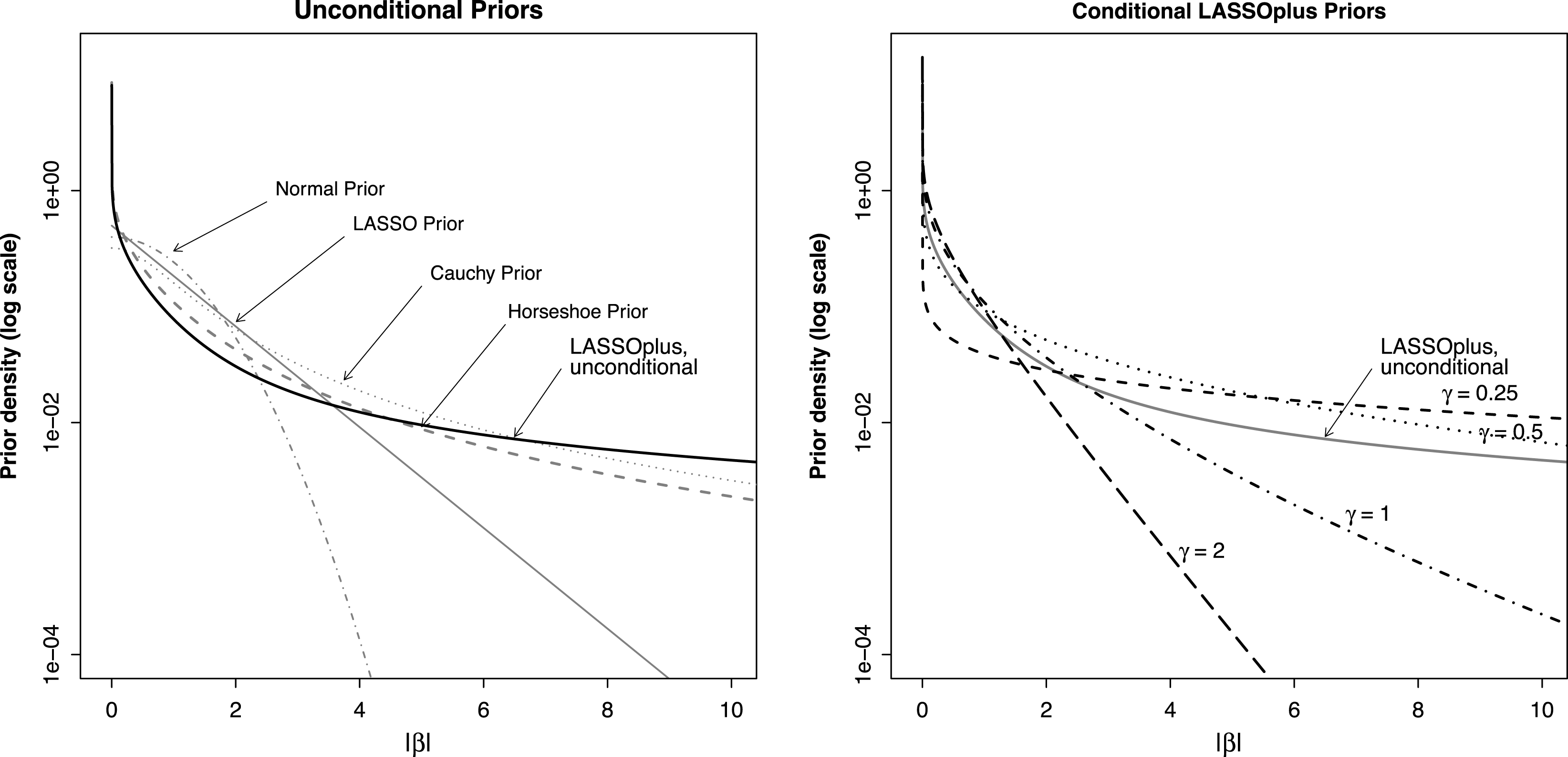
Comparison of Priors. This figure compares our unconditional LASSOplus prior to other priors (left) and shows the behavior of our conditional LASSOplus prior under different values of
 $\unicode[STIX]{x1D6FE}$
(right). The
 $x$
-axis contains values of
 $\unicode[STIX]{x1D6FD}$
and the
 $y$
-axis contains the prior density,
 $\Pr (\unicode[STIX]{x1D6FD})$
, on a log scale. We also include the two limiting distributions of the
 $t$
density, the normal and Cauchy, as well as the LASSO and horseshoe priors. The sparse priors (LASSO, horseshoe, LASSOplus) place greater mass at zero than the normal, an effect particularly pronounced for the horseshoe and LASSOplus priors. The normal prior places the least mass, and enacts the most shrinkage, on large effects. LASSOplus has the fattest tails, and thereby will have the least impact on posterior inference for large effects. The right-hand plot shows how the decay parameter
 $\unicode[STIX]{x1D6FE}$
affects the conditional prior,
 $\text{Pr}(\unicode[STIX]{x1D6FD}|\unicode[STIX]{x1D6FE})$
. The larger
 $\unicode[STIX]{x1D6FE}$
, the more aggressive the shrinkage. For smaller
 $\unicode[STIX]{x1D6FE}$
, the more the model is adjusting to large effects. As
 $\unicode[STIX]{x1D6FE}$
increases, less mass is placed in the tails and more toward zero. The parameter
 $\unicode[STIX]{x1D6FE}$
is estimated endogenously within the model.

Our model differs from earlier implementations of adaptive weights from Leng et al. (Reference Leng, Tran and Nott2014), Alhamzawi et al. (Reference Alhamzawi, Yu and Benoit2012), Griffin and Brown (Reference Griffin and Brown2012, Reference Griffin and Brown2010), Kang and Guo (Reference Kang and Guo2009) by placing a prior over
 $w_{k}^{\unicode[STIX]{x1D6FE}}$
rather than
 $w_{k}$
and
 $\unicode[STIX]{x1D6FE}$
separately. Like existing methods, we estimate the decay parameter
 $\unicode[STIX]{x1D6FE}$
from the data. As we show in Figure 1, adjusting the parameter allows the model to adapt to the global level of sparsity in the data. Taking
 $w_{k}=1$
for all
 $k$
returns the Bayesian LASSO model prior structure on
 $\unicode[STIX]{x1D6FD}_{k}$
;Footnote
13
this model is the implementation of LASSOplus that does not have the Oracle Property.
3.2 Estimation
Estimation is nearly identical to the augmented PC model. We augment the model as
 $$\begin{eqnarray}\displaystyle \unicode[STIX]{x1D6FD}_{k}|\unicode[STIX]{x1D706},w_{k},\unicode[STIX]{x1D70E}\sim DE(\unicode[STIX]{x1D706}w_{k}/\unicode[STIX]{x1D70E})\Rightarrow \unicode[STIX]{x1D6FD}_{k}|\unicode[STIX]{x1D70F}_{k}^{2},\unicode[STIX]{x1D70E}^{2},w_{k}^{2}\sim {\mathcal{N}}(0,\unicode[STIX]{x1D70F}_{k}^{2}\unicode[STIX]{x1D70E}^{2}/w_{k}^{2});\;\;\unicode[STIX]{x1D70F}_{k}^{2}\sim \exp (\unicode[STIX]{x1D706}^{2}/2). & & \displaystyle\end{eqnarray}$$
There are only two adjustments to the PC Gibbs sampler:
 $$\begin{eqnarray}\displaystyle \unicode[STIX]{x1D706}^{2}|\cdot & {\sim} & \displaystyle \unicode[STIX]{x1D6E4}\left(K\sqrt{N},\mathop{\sum }_{k=1}^{K}\unicode[STIX]{x1D70F}_{k}^{2}/2+\unicode[STIX]{x1D70C}\right)\end{eqnarray}$$
 $$\begin{eqnarray}\displaystyle 1/\unicode[STIX]{x1D70F}_{k}^{2}|\cdot & {\sim} & \displaystyle \text{InvGaussian}\left(\unicode[STIX]{x1D706}w_{k}\unicode[STIX]{x1D70E}/(|\unicode[STIX]{x1D6FD}_{k}|),\unicode[STIX]{x1D706}^{2}w_{k}^{2}\right).\end{eqnarray}$$
We update
 $w_{k}$
and
 $\unicode[STIX]{x1D6FE}$
using a Griddy Gibbs sampler (Tierney Reference Tierney1994).
3.3 The LASSOplus estimator
As with existing methods, the data-generating process above does not return a sparse mode. The LASSOplus estimate is constructed from the estimate
 $\unicode[STIX]{x1D6FD}_{k}$
and a thresholding function that zeroes out sufficiently small values of
 $|\unicode[STIX]{x1D6FD}_{k}|$
. The threshold was constructed such that the final estimate achieves the Oracle Property, a point we return to after defining the estimator itself.
In order to guarantee that we zero out effects in the limit of
 $N$
, we sample an inflated variance component,
 $\unicode[STIX]{x1D70E}_{sp}^{2}$
 $$\begin{eqnarray}\displaystyle \unicode[STIX]{x1D70E}_{sp}^{2}|\cdot \sim \text{InvGamma}\left(\left(N^{1-2\unicode[STIX]{x1D6FC}}-1\right)/2+K/2,\frac{1}{2}\left\{\mathop{\sum }_{i=1}^{N}(Y_{i}-X_{i}^{\top }\unicode[STIX]{x1D6FD})^{2}+\mathop{\sum }_{k=1}^{K}\unicode[STIX]{x1D6FD}_{k}^{2}/\unicode[STIX]{x1D70F}_{k}^{2}\right\}\right) & & \displaystyle\end{eqnarray}$$
that will enter into the threshold function. The parameter
 $\unicode[STIX]{x1D70E}_{sp}$
, which is central to the theoretical properties of LASSOplus, grows approximately as
 $N^{\unicode[STIX]{x1D6FC}}\unicode[STIX]{x1D70E}_{}$
. We implement the model at
 $\unicode[STIX]{x1D6FC}=1/4$
, as this value achieves several desirable theoretical properties as we explain below.
The LASSOplus estimate is constructed from the consistent model and the inflated variance term
 $\unicode[STIX]{x1D70E}_{sp}$
. Define as
 $$\begin{eqnarray}\displaystyle V_{i}^{k}=Y_{i}-X_{i,-k}^{\top }\unicode[STIX]{x1D6FD}_{-k} & & \displaystyle\end{eqnarray}$$
the outcome less the estimated values from all effects except the
 $k$
th. Next, denote the conditional least squares estimate
 $\widehat{\unicode[STIX]{x1D6FD}}_{k}^{ols}$
as
 $$\begin{eqnarray}\displaystyle \widehat{\unicode[STIX]{x1D6FD}}_{k}^{ols}=\frac{\mathop{\sum }_{i=1}^{N}X_{ik}V_{i}^{k}}{\mathop{\sum }_{i=1}^{N}X_{ik}^{2}}. & & \displaystyle\end{eqnarray}$$
Conditional on all other parameters in both models, the LASSOplus estimate for the
 $k$
th element is then defined as
 $$\begin{eqnarray}\displaystyle \unicode[STIX]{x1D6FD}_{k}^{plus}|\cdot =\unicode[STIX]{x1D6FD}_{k}\mathbf{1}\left(|\widehat{\unicode[STIX]{x1D6FD}}_{k}^{ols}|\geqslant \frac{\unicode[STIX]{x1D706}_{}\unicode[STIX]{x1D70E}_{sp}w_{k}}{N-1}\right). & & \displaystyle\end{eqnarray}$$
As LASSOplus is a Bayesian model, it returns estimates of the full posterior for all parameters. In the examples below, we select and focus on effects for which the median of the posterior density is nonzero,
 $\text{med}(\unicode[STIX]{x1D6FD}_{k}^{plus}|\cdot )\neq 0$
. We show that selecting off the median LASSOplus estimates serves as a conservative and powerful rule when trying to identify nonzero effects.
3.4 Approximate confidence intervals
A crucial contribution of LASSOplus is uncertainty estimates for model parameters. While the LASSOplus method returns posterior uncertainty estimates, the following discussion shows how to calculate approximate confidence intervals. We focus on confidence intervals because credible intervals are not calibrated to achieve nominal coverage, except in the limit. And as with earlier work, we found coverage to be subnominal with credible intervals (Kyung et al. Reference Kyung, Gill, Ghosh and Casella2010).
In returning approximate confidence intervals, we sample from the approximate sampling distribution of the LASSOplus estimator. To do so, we approximate Equation (44) as
 $$\begin{eqnarray}\displaystyle \unicode[STIX]{x1D6FD}_{k}^{plus}|\cdot \approx \unicode[STIX]{x1D6FD}_{k}\boldsymbol{\unicode[STIX]{x1D6F7}}\left(\left|\frac{\widehat{\unicode[STIX]{x1D6FD}}_{k}^{ols}}{\widehat{\unicode[STIX]{x1D70E}}_{k}}\right|\geqslant \frac{\unicode[STIX]{x1D706}_{}\unicode[STIX]{x1D70E}_{sp}w_{k}}{\widehat{\unicode[STIX]{x1D70E}}_{k}(N-1)}\right) & & \displaystyle\end{eqnarray}$$
with
 $\widehat{\unicode[STIX]{x1D70E}}_{k}$
the variance of
 $\unicode[STIX]{x1D6FD}_{k}^{ols}$
. We apply the delta method to estimate
 $\unicode[STIX]{x1D70E}_{ci}^{2}$
(see the online supplemental materials for details and Efron (Reference Efron2015) for a more general argument).
The asymptotic normal approximation of the delta method may not hold with small samples. To correct for this, we estimate the error degrees of freedom using Satterthwaite’s approximation,
 $$\begin{eqnarray}\displaystyle df^{ci}=\frac{\left(\mathop{\sum }_{i=1}^{N}(Y_{i}-X_{i}^{\top }\unicode[STIX]{x1D6FD})^{2}\right)^{2}}{\mathop{\sum }_{i=1}^{N}(Y_{i}-X_{i}^{\top }\unicode[STIX]{x1D6FD})^{4}}. & & \displaystyle\end{eqnarray}$$
With an estimate of error degrees of freedom in hand, we exploit the representation of a
 $t$
-density as a scale mixture of normals with inverse-gamma mixing density. We draw
 $v_{ci}\sim \text{InvGamma}(df^{ci}/2,df^{ci}/2)$
and use this value to inflate
 $\unicode[STIX]{x1D70E}_{ci}^{2}$
.Footnote
14
The sampling density of a nonzero univariate LASSO estimate is truncated-normal, conditional on the sign of the mode (Potscher and Leeb Reference Potscher and Leeb2009). Our approximation of the sampling density is then
 $$\begin{eqnarray}\displaystyle \unicode[STIX]{x1D6FD}_{k}^{ci}|\cdot \sim \left\{\begin{array}{@{}l@{}}{\mathcal{N}}\left(\unicode[STIX]{x1D6FD}_{k}^{plus},\unicode[STIX]{x1D70E}_{ci}^{2}v_{ci}\right);\quad \unicode[STIX]{x1D6FD}_{k}^{plus}=0\quad \\ {\mathcal{T}}{\mathcal{N}}\left(\unicode[STIX]{x1D6FD}_{k}^{plus},\unicode[STIX]{x1D70E}_{ci}^{2}v_{ci},0,\infty \right);\quad \unicode[STIX]{x1D6FD}_{k}^{plus}>0\quad \\ {\mathcal{T}}{\mathcal{N}}\left(\unicode[STIX]{x1D6FD}_{k}^{plus},\unicode[STIX]{x1D70E}_{ci}^{2}v_{ci},-\infty ,0\right);\quad \unicode[STIX]{x1D6FD}_{k}^{plus}<0\quad \end{array}\right. & & \displaystyle\end{eqnarray}$$
where
 ${\mathcal{T}}{\mathcal{N}}(\unicode[STIX]{x1D707},\unicode[STIX]{x1D70E}^{2},l,u)$
denotes the truncated-normal density with mean
 $\unicode[STIX]{x1D707}$
, variance
 $\unicode[STIX]{x1D70E}^{2}$
, and support on
 $(l,u)$
.
The approximate confidence interval is taken from the posterior distribution of
 $\unicode[STIX]{x1D6FD}_{k}^{ci}$
. For
 $K$
discovered effects, we take
 $\widetilde{K}=\max (K,1)$
and approximate the
 $1-\unicode[STIX]{x1D6FC}_{0}\%$
confidence interval as
 $$\begin{eqnarray}\displaystyle CI_{\unicode[STIX]{x1D6FC}_{0},\widetilde{K}}=\left(q_{\unicode[STIX]{x1D6FC}_{0}/(2\widetilde{K})},q_{1-\unicode[STIX]{x1D6FC}_{0}/(2\widetilde{K})}\right) & & \displaystyle\end{eqnarray}$$
where
 $q_{\widetilde{\unicode[STIX]{x1D6FC}}}$
is the estimated
 $\widetilde{\unicode[STIX]{x1D6FC}}$
quantile of
 $\unicode[STIX]{x1D6FD}_{k}^{ci}$
, with a Bonferroni correction for the discovered effects. Benjamini and Yekutieli (Reference Benjamini and Yekutieli2005, esp. 74–75) show that implementing a Bonferroni correction off discovered effects will maintain at least nominal coverage across all discovered effects.
3.5 Random effects and uncertainty estimates for designs using repeated unit-level observations
When researchers have repeated units in their sample, ignoring within-unit correlation can produce incorrect uncertainty estimates. Our substantive application, which uses a conjoint experiment by design, features repeated observations at the unit level. Often researchers will utilize some form of clustered standard errors. LASSOplus implements unit-level random effects for the same purpose.Footnote 15
Specifically, assume observation
 $i\in \{1,2,\ldots ,N\}$
as above. Now, assume each observation was generated by experimental unit
 $j$
,
 $j\in \{1,2,\ldots ,J\}.$
The function
 $j[i]$
maps each observation back to one of the experimental units (Gelman and Hill Reference Gelman and Hill2007).
We include random effects
 $u_{i}$
as
 $$\begin{eqnarray}\displaystyle u_{i} & = & \displaystyle a_{j[i]}\end{eqnarray}$$
 $$\begin{eqnarray}\displaystyle a_{j[i]} & {\sim} & \displaystyle {\mathcal{N}}(0,\unicode[STIX]{x1D70E}_{a}^{2}).\end{eqnarray}$$
We take the Jeffreys’ prior
 $1/\unicode[STIX]{x1D70E}^{2}$
on
 $\unicode[STIX]{x1D70E}^{2}$
, though a folded-
 $t$
density may be used (Gelman Reference Gelman2006).
3.6 Parametric extensions
Most experimental studies implement a linear (mean) model, given its connection to causal estimands. Researchers may prefer alternative models however, such as a probit model for a binary outcome. In this case, LASSOplus models this alternative data-generating process in a straightforward way by using the latent variable representation of the probit model (Albert and Chib Reference Albert and Chib1993). Briefly, the probit regression models the probability of a positive outcome as
 $$\begin{eqnarray}\displaystyle \Pr (Y_{i}=1|X_{i},\unicode[STIX]{x1D6FD})=\unicode[STIX]{x1D6F7}(X_{i}^{\top }\unicode[STIX]{x1D6FD}) & & \displaystyle\end{eqnarray}$$
with
 $\unicode[STIX]{x1D6F7}(a)$
representing the cumulative distribution for a standard normal random variable. An observation-specific random variable is introduced,
 $z_{i}^{\ast }$
, and the problem transforms to
 $$\begin{eqnarray}\displaystyle z_{i}^{\ast }=X_{i}^{\top }\unicode[STIX]{x1D6FD}+e_{i} & & \displaystyle\end{eqnarray}$$
with
 $e_{i}\stackrel{\text{i.i.d.}}{{\sim}}{\mathcal{N}}(0,1)$
. Conditional on
 $z_{i}^{\ast }$
, the probit regression is a least squares problem with known variance, and LASSOplus can be applied as above. The latent variable representation also allows straightforward extension to ordinal, categorical, and censored data (Jackman Reference Jackman2009).
3.7 Expectation–maximization implementation
While we have certainly worked to produce an efficient implementation of LASSOplus, the MCMC method given above may be time-consuming and computationally expensive for large datasets with a large number of possible effects. For practical research and initial model fitting, we also implement an EM version of the LASSOplus model. We take
 $\unicode[STIX]{x1D6FD},\unicode[STIX]{x1D70E}^{2}$
as the parameters to be estimated and the remaining parameters,
 $\{\unicode[STIX]{x1D706},\{1/\unicode[STIX]{x1D70F}_{k}^{2}\}_{k=1}^{K},\{w_{k}\}_{k=1}^{K},\unicode[STIX]{x1D6FE}\}$
, as “missing.”Footnote
16
As we have calculated all of the conditional posterior densities or kernels, the EM implementation is straightforward. We defer the details to the online supplemental materials.
4 Statistical Properties of LASSOplus
In this section, we discuss the statistical properties of LASSOplus. First, we present some preliminary results that will be used in later results. Second, we derive conditions under which LASSOplus satisfies the Oracle Property, in both a fixed-
 $K$
and growing-
 $K$
setting. Third, we give Oracle Inequality bounds for both the consistent model and LASSOplus. As the Oracle Inequality is a frequentist property, we derive these results in terms of the LASSOplus-EM estimates. Fourth, we compare the LASSOplus prior to several existing Bayesian priors.
4.1 Preliminary results
We present here two preliminary results. First, we consider the role of the weights,
 $\widehat{w}_{k}$
. Each weight is associated with a parameter in the penalty, where we want to downweight the penalty associated with large effects and upweight the penalty associated with small effects. We first show that the weights and magnitude of the effect estimates are indeed inversely related.
Lemma 2. The partial derivative of
 $\widehat{w}_{k}$
with respect to
 $|\widehat{\unicode[STIX]{x1D6FD}}_{k}|$
is
 $$\begin{eqnarray}\displaystyle \frac{\unicode[STIX]{x2202}\widehat{w}_{k}}{\unicode[STIX]{x2202}|\widehat{\unicode[STIX]{x1D6FD}}_{k}|}=-\widehat{\unicode[STIX]{x1D706}}\sqrt{\widehat{\frac{1}{\unicode[STIX]{x1D70E}^{2}}}}\text{Var}(w_{k}|\cdot ) & & \displaystyle\end{eqnarray}$$
which is strictly less than zero.
Proof. See the online supplemental materials.
This will allow us to associate the largest weights with the smallest effect estimates, and vice versa.
Second, we bound
 $\widehat{\unicode[STIX]{x1D706}}$
:
Lemma 3. When
 $N$
and
 $K$
grow at some rate,
 $\widehat{\unicode[STIX]{x1D706}}$
grows as
 $N^{1/4}K^{1/2}$
.
Proof. See the online supplemental materials.
The bound on
 $\widehat{\unicode[STIX]{x1D706}}$
is a crucial component of both proofs below, as the growth rate of
 $\widehat{\unicode[STIX]{x1D706}}$
and
 $\widehat{w}_{k}$
determine the LASSOplus-EM estimator and, hence, its statistical properties. We turn next to the first result.
4.2 Oracle Property and Oracle Inequality for LASSOplus
We now give conditions on
 $N,K$
for which LASSOplus achieves the Oracle Property. We then show that both the estimator from the consistent model and LASSOplus each satisfy their own Oracle Inequality.
4.2.1 Oracle Property of the LASSOplus estimator
As described above in Section 2.5, an estimator that satisfies the Oracle Property meets two conditions. First, it is consistent for variable selection, so in-truth nonzero effects selected and in-truth zero effects are zeroed out. Second, the estimate has to be indistinguishable asymptotically from a consistent, asymptotically efficient, model fit only to the in-truth nonzero effects. In other words, the estimator achieves the same performance as an identical estimator told ex ante by an “oracle” which effects are zero and which are not.
The LASSOplus estimator satisfies both properties in the case of a fixed
 $K$
and
 $\lim _{N\rightarrow \infty }$
, and hence is an Oracle estimator. We offer the following:
Proposition 3 (Oracle Property of LASSOplus).
Whenever
 $K$
is growing in
 $N$
, but
 $K^{2}/N\rightarrow 0$
, and
 $1/4\leqslant \unicode[STIX]{x1D6FC}<1$
, LASSOplus has the two Oracle Properties:
1. Consistent Variable Selection:
$\lim _{N\rightarrow \infty }\{k:\Pr (\widehat{\unicode[STIX]{x1D6FD}}_{k}^{plus}\neq 0)=1\}=S$
.2. Optimal Estimation Rate:
$\sqrt{N}(\widehat{\unicode[STIX]{x1D6FD}}_{S}^{plus}-\unicode[STIX]{x1D6FD}_{S}^{o})\stackrel{\text{d}}{\rightarrow }{\mathcal{N}}(\mathbf{0}_{|S|},\unicode[STIX]{x1D6F4}_{S}^{\ast })$
where
$\unicode[STIX]{x1D6F4}_{S}^{\ast }$
is the asymptotic variance matrix from the true subset model


with
 $S$
the set of indices of in-truth nonzero elements of
 $\unicode[STIX]{x1D6FD}$
, i.e.
 $S=\{k:k\in \unicode[STIX]{x1D6FD}_{k}^{o}\neq 0\}$
, and.
 $V_{S}$
the asymptotic variance of the least squares estimator fit only to the in-truth nonzero effects.
These properties also hold in the fixed-
 $K$
setting when
 $1/4<\unicode[STIX]{x1D6FC}<1.$
Proof. See Appendix A.
Our result of
 $K^{2}/N\rightarrow 0$
is much weaker than that of Fan and Peng (Reference Fan and Peng2004), who require
 $K^{5}/N\rightarrow 0$
.Footnote
17
This difference appears because Fan and Peng (Reference Fan and Peng2004) prove their result in some generality, for general likelihoods and penalties, whereas we are using a normal likelihood and have a particular penalty function.
4.2.2 Oracle Inequality of the LASSOplus estimator
We next present an Oracle Inequality for the LASSOplus-EM model, which we formally prove in Appendix B. Standard Oracle Inequality results generally involve controlling a probabilistic bound on the distance between the estimated and true regression parameters. As LASSOplus-EM recovers the mode of a Bayesian model, the probability in the bound is not controlled by the researcher; it is instead estimated endogenously along with all other parameters. We find that both the consistent model and LASSOplus satisfy an Oracle Inequality.
The Oracle Inequalities below offer two heuristic insights. First, the consistent model performs well with prediction when
 $N$
is of order
 $(K/log(K))^{2}$
or less. Therefore, the consistent model does well when predicting in small-
 $N$
, large-
 $K$
settings. Second, LASSOplus satisfies an Oracle Inequality so long as
 $K$
is growing, and regardless of
 $N$
. This comes at the cost of a bound that is twice that of the consistent model.
4.2.3 Formal statement of the LASSOplus Oracle Inequality
We state the results here but defer the full set of definitions and derivations to Appendix B. The interested reader will find there all definitions and assumptions, though we note that the practical insights from the theoretical derivations are described directly above.
Denote as
 $\widehat{W}$
the matrix with the weights along the diagonal;
 $C_{\cdot }$
, i.e.
 $C_{\unicode[STIX]{x1D706}}$
,
 $C_{\unicode[STIX]{x1D716}}$
, etc., as constants not changing in
 $N$
or
 $K$
;
 $\widehat{\overline{\unicode[STIX]{x1D6FE}}}$
the maximal value that can be taken by a weight;
 $|\widehat{S}|$
is the estimated number of large effects; and
 $p_{\unicode[STIX]{x1D706}}(C_{\unicode[STIX]{x1D706}})$
,
 $p_{\unicode[STIX]{x1D716}}(C_{\unicode[STIX]{x1D716}})$
, and
 $p_{w}(C_{1},C_{2},C_{3})$
the probabilities with which necessary bounds are violated. The parameter
 $t$
is a user-selected term that controls the error, such that the probability that the bound contains a term
 $\exp (-t^{2}/2)$
.
Proposition 4 (Oracle Inequality for LASSOplus).
The LASSOplus-EM model offers two separate Oracle Inequality results.
Denote as
 $\widehat{\unicode[STIX]{x1D6FF}}=\widehat{\unicode[STIX]{x1D6FD}}-\unicode[STIX]{x1D6FD}^{o}$
and
 $\widehat{\unicode[STIX]{x1D6FF}}^{P}$
the subvector of
 $\widehat{\unicode[STIX]{x1D6FF}}$
corresponding to effects not zeroed out by LASSOplus. Similarly, let
 $X_{p}$
and
 $\widehat{W}_{p}$
denote the submatrices of
 $X$
and
 $\widehat{W}$
associated with elements of
 $\widehat{\unicode[STIX]{x1D6FF}}^{p}$
. Then, under the assumptions in Appendix B,
1. So long as
(54)the consistent model will satisfy the Oracle Inequality$$\begin{eqnarray}\displaystyle 32\times \sqrt{(N-1)}\leqslant \frac{C_{\unicode[STIX]{x1D706}}C_{\unicode[STIX]{x1D716}}C_{2}\widehat{\overline{\unicode[STIX]{x1D6FE}}}^{2}K}{\frac{t^{2}}{2}+\log (K-|\widehat{S}|)} & & \displaystyle\end{eqnarray}$$
(55)with probability at least$$\begin{eqnarray}\displaystyle \frac{1}{N}\left\{\Vert X\widehat{\unicode[STIX]{x1D6FF}}\Vert _{2}^{2}+\unicode[STIX]{x1D706}\widehat{\unicode[STIX]{x1D70E}}\Vert \widehat{W}\widehat{\unicode[STIX]{x1D6FF}}\Vert _{1}^{1}\right\}\leqslant \frac{C_{L1}\widehat{\unicode[STIX]{x1D70E}}^{2}\widehat{\unicode[STIX]{x1D706}}^{2}|S|}{N^{2}\left\{C_{\unicode[STIX]{x1D719}_{1}}\frac{\widehat{\unicode[STIX]{x1D706}}^{2}\widehat{\unicode[STIX]{x1D70E}}^{2}\widehat{\unicode[STIX]{x1D6FD}}_{(K)}^{2}}{\text{}\underline{C}_{1}\log (|\widehat{S}|)^{2}}+C_{\unicode[STIX]{x1D719}_{2}}C_{2}\widehat{\overline{\unicode[STIX]{x1D6FE}}}\right\}^{2}} & & \displaystyle\end{eqnarray}$$
$1-\exp (-t^{2}/2)-p_{\unicode[STIX]{x1D706}}(C_{\unicode[STIX]{x1D706}})-p_{\unicode[STIX]{x1D716}}(C_{\unicode[STIX]{x1D716}})-p_{w}(C_{1},C_{2},C_{3})$
.2. So long as
(56)$$\begin{eqnarray}\displaystyle \frac{C_{\unicode[STIX]{x1D706}}C_{\unicode[STIX]{x1D716}}C_{2}\widehat{\overline{\unicode[STIX]{x1D6FE}}}^{2}K}{\frac{t^{2}}{2}+\log (K-|\widehat{S}|)}\geqslant 32 & & \displaystyle\end{eqnarray}$$
$\widehat{\unicode[STIX]{x1D6FD}}^{plus}$
satisfies an Oracle Inequality. (57)with probability at least$$\begin{eqnarray}\displaystyle \frac{1}{N}\left\{\Vert X_{p}\widehat{\unicode[STIX]{x1D6FF}}^{p}\Vert _{2}^{2}+\unicode[STIX]{x1D706}\widehat{\unicode[STIX]{x1D70E}}|\widehat{W}_{p}\widehat{\unicode[STIX]{x1D6FF}}^{p}|_{1}^{1}\right\}\leqslant 2\frac{C_{L1}\widehat{\unicode[STIX]{x1D70E}}^{2}\widehat{\unicode[STIX]{x1D706}}^{2}|S|}{N^{2}\left\{C_{\unicode[STIX]{x1D719}_{1}}\frac{\widehat{\unicode[STIX]{x1D706}}^{2}\widehat{\unicode[STIX]{x1D70E}}^{2}\widehat{\unicode[STIX]{x1D6FD}}_{(K)}^{2}}{\text{}\underline{C}_{1}\log (|\widehat{S}|)^{2}}+C_{\unicode[STIX]{x1D719}_{2}}C_{2}\widehat{\overline{\unicode[STIX]{x1D6FE}}}\right\}^{2}} & & \displaystyle\end{eqnarray}$$
$1-\exp (-t^{2}/2)-p_{\unicode[STIX]{x1D706}}(C_{\unicode[STIX]{x1D706}})-p_{\unicode[STIX]{x1D716}}(C_{\unicode[STIX]{x1D716}})-p_{w}(C_{1},C_{2},C_{3})$
.


Proof. See Appendix B.
The Oracle Inequality offers insight when
 $K>N$
, and LASSOplus performs well in this setting. We next move on to a comparative look at LASSOplus from a Bayesian perspective.
4.3 Comparison to existing priors
The Oracle Property and Oracle Inequality are both theoretical results. As we designed LASSOplus for use on real data, we next move on to finite-sample consideration by examining the behavior of the prior structure over the parameter weights
 $w_{k}$
. This enables us to compare the prior used in LASSOplus to other priors used in the literature.
There is, of course, no prior structure that performs well in all situations and for all data sets. We have generated a prior structure with four properties. First, the prior is concentrated at zero. This is appropriate for a setting where the researcher confronts hundreds or thousands of effects and wants to winnow these down to a small subset of relevant ones. Second, the prior places a large probability on the existence of large effects. For example, a standard normal prior places a
 $5.0\%$
prior probability on observing a value larger than 1.96 in magnitude. For a Cauchy prior, this value is
 $30.0\%$
; for the horseshoe,
 $20.0\%$
, and for LASSOplus,
 $31.39\%$
. The more mass in the tails, the less posterior inference on large effects will be impacted by the prior. Third, the decay parameter
 $\unicode[STIX]{x1D6FE}$
allows the prior to adjust to the level of sparsity implied by the data. Fourth, the prior is less informative than several existing sparse priors. Conditional on assuming a sparse model, we want a prior that drives posterior inference as little as possible.
We illustrate the properties of the LASSOplus prior in Figure 1.Footnote
18
In each plot, the
 $y$
-axis contains the prior probability on a log scale and the
 $x$
-axis contains the magnitude of the effect,
 $|\unicode[STIX]{x1D6FD}|$
. The left figure plots the unconditional LASSOplus prior
 $$\begin{eqnarray}\displaystyle \text{Pr}(\unicode[STIX]{x1D6FD})=\int \Pr (\unicode[STIX]{x1D6FD}|\unicode[STIX]{x1D6FE})\Pr (\unicode[STIX]{x1D6FE})d\unicode[STIX]{x1D6FE} & & \displaystyle\end{eqnarray}$$
against the normal, LASSO (double exponential), Cauchy, and horseshoe priors.
The left-hand plot in Figure 1 illustrates how the different priors will handle large, intermediate, and small effects. The LASSOplus, LASSO, and horseshoe priors all concentrate at zero relative to the normal and Cauchy. The LASSOplus and horseshoe have the most pronounced spike at zero, and therefore will be the most aggressive in shrinking small effects to zero. This suggests that the LASSOplus and horseshoe should make the fewest false positive discoveries. LASSOplus is also relatively aggressive in shrinking intermediate effects to zero. For example, the normal prior places a high mass on effects less than 2 in magnitude, and will therefore shrink those the least. For larger values, say much larger than 4 in magnitude, the normal prior places a vanishingly low probability and will therefore shrink effect estimates quite a bit. The horseshoe and LASSO both place a higher mass on intermediate effects less than approximately 4 in magnitude. This suggests that the horseshoe and LASSO are more likely to discover intermediate effects, and that the LASSOplus will be relatively conservative in this range. We find this behavior in the simulations below. The horseshoe, LASSOplus, and Cauchy all have fatter tails than the LASSO and normal. Of these three, the LASSOplus has the fattest tails, and therefore will have the least impact on posterior inference for large effects.
The right-hand plot in Figure 1 shows how the decay parameter
 $\unicode[STIX]{x1D6FE}$
affects the conditional prior,
 $\text{Pr}(\unicode[STIX]{x1D6FD}|\unicode[STIX]{x1D6FE})$
. For a larger
 $\unicode[STIX]{x1D6FE}$
, the more aggressive the shrinkage is. For smaller
 $\unicode[STIX]{x1D6FE}$
, the more the model is adjusting to large effects. As
 $\unicode[STIX]{x1D6FE}$
increases, less mass is placed in the tails and more toward zero. The parameter
 $\unicode[STIX]{x1D6FE}$
is estimated endogenously within the model.
Another way to evaluate different prior distributions is to compare the amount of information they contribute to posterior inference. Practitioners are naturally wary of results driven by prior assumptions. A long strand of research has sought to identify reference priors such that the resultant posterior is dominated by the data (see particularly Bernardo Reference Bernardo1979; Jaynes Reference Jaynes1982; Berger and Bernardo Reference Berger and Bernardo1989; Bernardo Reference Bernardo, Dey and Rao2005; Berger et al.
Reference Berger, Bernardo and Sun2009; Berger Reference Berger2006). A standard measure of the information in a prior
 $p$
with support
 ${\mathcal{B}}$
is its entropy, with higher values indicating less prior influence on the posterior:Footnote
19
 $$\begin{eqnarray}\displaystyle H(p)=-\int _{{\mathcal{B}}}p(\unicode[STIX]{x1D6FD})\log \left(p(\unicode[STIX]{x1D6FD})\right)d\unicode[STIX]{x1D6FD}. & & \displaystyle\end{eqnarray}$$
The reference prior is the prior from a class of densities that maximizes the entropy. For a single-parameter, asymptotically normal posterior, the reference prior is the Jeffreys’ prior.
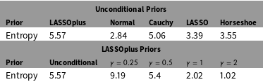
We present the entropy of the priors in Table 1. The unconditional LASSOplus has the highest entropy among sparse priors (LASSO, horseshoe). The unconditional LASSOplus even has higher entropy than the Cauchy, which is proper but has no finite moments. Among the conditional LASSOplus priors, smaller values of
 $\unicode[STIX]{x1D6FE}$
correspond with a larger entropy. In the absence of information about expected effect size and the underlying level of sparsity, we prefer the conditional LASSOplus prior with the global decay parameter
 $\unicode[STIX]{x1D6FE}$
estimated from the data.
Comparison of Entropy Across Priors. From an objective Bayesian viewpoint, priors with a higher entropy are favored. Higher-entropy priors, intuitively, add less information to the model and have less impact on posterior inference. We present the entropy of the priors shown in Figure 1. The unconditional LASSO plus has the highest entropy among the unconditional priors. Among the conditional LASSOplus priors, smaller values of
 $\unicode[STIX]{x1D6FE}$
correspond with a larger entropy. In the absence of information about expected effect size, we prefer the conditional LASSOplus prior with the global decay parameter
 $\unicode[STIX]{x1D6FE}$
estimated from the data.

5 Application to Subgroup Analysis
Though broadly applicable in a regression framework, we developed LASSOplus for use with subgroup analysis. We discuss next several issues that arise when using the method for subgroup analysis, and how our implementation helps address some of these concerns.
5.1 Subgroup analysis through repeatedly split sample analyses
In experimental analyses, subgroup analysis often consists of analysis of repeatedly split samples. For example, authors may conduct a long series of subgroup analyses by splitting the sample into different groups based on one dichotomous or dichotomized pretreatment covariate at a time. A regression model is fit to each group, and then the marginal effects of the different effects are evaluated within each subsample.
While showing these interactions between treatment conditions and pretreatment covariates is theoretically interesting, and often requested by audience members and reviewers, the methodology employed has a number of limitations. The decision to split subgroups one at a time introduces both conceptual and statistical concerns. Conceptually, the decision to conduct multiple separate subgroup analyses means that we implicitly acknowledge that we have estimated the wrong model. Take for example the simple moderating effects of two separate pretreatment variables on a treatment effect. The fact that the moderating effect of one of these variables is not included when estimating the moderating influence of another variable implies an awareness of potential misspecification. Statistically, the decision to conduct multiple separate subgroup analyses by discarding part of the data each time means the estimates are inefficient. This can be remedied by allowing for interactions between the treatment condition and the covariate in the same model. But the proliferation of parameters means that the standard regression framework is ill-equipped to deal with these situations. The basic reason is simple: the number of parameters quickly proliferates and hence some sort of stabilization, such as through sparsity, is necessary. We illustrate the advantages of sparsity-inducing priors below.
5.2 Interpreting interaction terms and the sparsity assumption
We use LASSOplus to estimate saturated models containing tens, hundreds, or even thousands of interaction terms. Common, and correct, practice proscribes including interaction terms in the absence of lower-order terms. We agree. Our implementation of LASSOplus, at its default, fits a model with all lower-order and interaction terms.
We also want to address the concern that the proposed methodology works only under the assumption that most of the effects are in truth zero. This assumption may arise from the frequentist implementation of the LASSO, whose proponents argue for using the “bet on sparsity principle” (Hastie et al. Reference Hastie, Tibshirani and Friedman2010, p. 611–613), arguing that sparse models are to be preferred over dense models. However, we do not assume that the true effects are zero in any sense. Our prior places mass 0 at the point 0. This differs from spike-and-slab priors, where the researcher implicitly places some prior mass on each parameter being zero (Mitchell and Beauchamp Reference Mitchell and Beauchamp1988; O’Hara and Silanapaa Reference O’Hara and Silanapaa2009; Gill Reference Gill2014, ch. 4.6). Instead, we generate a summary of the posterior that takes the value zero with some nonzero probability, allowing the data to tell us ex post that some effect is negligible. We are not assuming that the true value, even after the model is fit, is zero—instead, we seek the best sparse representation of the outcome in terms of main and subgroup effects.
Furthermore, researchers interested in characterizing every effect are able to do so. The pseudoposterior density of each effect is not sparse, as illustrated in our applied example. Researchers interested in evaluating nonselected effects are able to do so by evaluating this full posterior density. An important step in any analysis is to look to the data to determine which variables have a nonnegligible effect. LASSOplus provides an answer to this question by returning posterior median estimates of zero for negligible variables.
Lastly, the researcher may be nervous in interpreting higher-order interaction terms when the lower-order terms are not selected. The reason is that standard interaction terms cannot be interpreted without referencing their lower-order terms. The problem of interpreting interactions arises because of a correlation between the lower-order terms and the interaction term: the effect of one cannot be considered independently of the other (Esarey and Summer Reference Esarey and Summer2015). To solve this problem, we include interactions terms that are uncorrelated with their lower-order terms. To do so, first we construct the interaction term through elementwise multiplication, regress this term on its lower-order terms, and enter the residuals from this regression into LASSOplus. Under this construction, the effects of interaction terms can be interpreted as the effect above and beyond any lower-order effects. For a proof, see the online supplemental materials.
5.3 Scope of method for subgroup analysis
The development of the LASSOplus method to, in part, facilitate subgroup analysis had two goals. The first is to allow the experimentalist to uncover potentially relevant subgroup effects after implementing an experiment. Second, we designed the method to apply from the simplest of experiments to a conjoint analysis with repeated observations. The analysis of experimental data normally occurs in two steps. An experiment is designed to test a set of prespecified hypotheses. Upon completing an experiment, these hypotheses are then tested, and the point estimates and
 $p$
-values for each effect are reported.
Our method is designed for use in the subsequent analysis. After the inferential stage, researchers may be interested in higher-order effects, including treatment heterogeneity, when two treatments have an interactive effect; treatment effect heterogeneity, when the effect of a treatment varies with a covariate; or targeted treatment effect, when the effect of a treatment interaction varies with a covariate (Imai and Ratkovic Reference Imai and Ratkovic2013). Common practice involves repeatedly subsetting the data on pretreatment covariates and running separate regressions in each subset. For example, the researcher may find no treatment effect on average, but may find effects of opposite signs for males and females in her experimental data. The problem is the sheer number of effects quickly overwhelms, and researcher-driven repeated subsetting quickly devolves into interaction fishing.
The proposed method provides a means for considering all possible interaction terms and returning a sparse subset estimated as nonzero. The estimation is postinferential and descriptive, returning the effects that seem pronounced in this experimental data and might be considered for further study in the next experiment.
6 Simulation Study
In this section, we compare LASSOplus to several sparse estimators, assessing each method in terms of discovery of all effects, discovery of small effects, and coverage. We find that LASSOplus performs competitively across each dimension.
6.1 Setup
Our simulation is motivated by conjoint experiments, where the researcher wants to search through a large number of treatment/covariate interactions. The simulation mimics an experiment with 3 treatments, having 2, 3, and 4 levels, respectively. We also assume a set of
 $p$
pretreatment covariates, with
 $p\in \{10,25,50,75,100\}$
. The design matrix consists of the matrix of treatment indicators,
 $T$
, the pretreatment covariates,
 $X^{0}$
, and their residualized interactions. We designate the first level of each treatment as the baseline, dropping it and all of its interactions from
 $X$
. After creating all interactions, we are left with a design matrix
 $X$
with one of
 $\{76,181,356,531,706\}$
covariates. We run simulations with sample sizes
 $N\in \{50,100,250,500,1000,2500\}$
. For 16/30 of our simulation setups (
 $53\%$
), we have more observations than covariates.
We assume the following model:
 $$\begin{eqnarray}\displaystyle E(Y_{i}|X_{i},T_{i1},T_{i2},T_{i3}) & \propto & \displaystyle 3X_{i2}+3X_{i3}+3X_{i4}\end{eqnarray}$$
 $$\begin{eqnarray}\displaystyle & & \displaystyle +\,2\times \mathbf{1}(T_{i2}=b)+2\times \mathbf{1}(T_{i3}=b)+2\times \mathbf{1}(T_{i3}=c)\end{eqnarray}$$
 $$\begin{eqnarray}\displaystyle & & \displaystyle +\,X_{i2}\times \mathbf{1}(T_{i2}=b)+X_{i2}\times \mathbf{1}(T_{i3}=c)+X_{i2}\times \mathbf{1}(T_{i2}=a)\end{eqnarray}$$
 $$\begin{eqnarray}\displaystyle & & \displaystyle +\,X_{i4}\times \mathbf{1}(T_{i1}=b)+X_{i3}\times \mathbf{1}(T_{i3}=b)+X_{i4}\times \mathbf{1}(T_{i3}=c)\end{eqnarray}$$
with noise from a
 $t_{5}$
density and the systematic component is scaled to give a true
 $R^{2}$
of 0.5. The variables in
 $X_{i}$
are drawn from a
 $\mathit{Wishart}_{p}(N)$
, and each treatment condition is equiprobable. Each simulation setting was run 1000 times. The simulation design mimics a situation where there a few large main effects, some medium-sized average treatment effects, and the remaining interaction terms are small relative to the other effects.
6.2 Alternative estimators
We compare LASSOplus to three alternative sparse estimators: the frequentist LASSO, frequentist adaptive LASSO, and the horseshoe estimator. The LASSO and adaptive LASSO are fit using glmnet from R package glmnet. First-stage estimates come from ridge regression with the tuning parameter selected to minimize cross-validated error. The horseshoe prior is implemented in STAN.Footnote
20
We coded up an implementation of LASSO
 $+$
OLS with all tuning parameters set at the defaults suggested by the original authors.
For details on the implementation of additional methods, see the online supplemental materials.
6.3 Results
A primary concern is differentiating relevant from irrelevant effects. As a secondary concern, estimators must be responsive to main effects as well as smaller subgroup effects. We first compare methods based on their ability to reliably pick up the former and not mislead on the latter. We consider all effects (Figure 2) and smaller interaction effects (Figure 3).
False Positive, False Negative, and False Discovery Rates, All Effects. Each row represents the results for a different number of effects. The sample size is along the
 $x$
-axis. LASSOplus achieves a lower false positive rate and false discovery rate across simulation settings (first and third columns), while still maintaining reasonable power in terms of the false negative rate (middle column).

Consider first the results for all effects, in Figure 2. The plots are arranged in rows by the number of possible effects, with the sample size along the
 $x$
-axis. Columns contain false positives (left), false negatives (center), and false discovery rates (right). Starting in the rightmost column, the LASSOplus has the lowest false positive rate across all settings except for the largest-
 $N$
, smallest-
 $K$
setting, where it is outperformed by the horseshoe. In terms of false negatives, consider first the setting with
 $K=76$
and
 $K=181$
. In this setting, the LASSOplus achieves a false negative rate either lower than or approximately the same as the horseshoe. As
 $K$
increases, the horseshoe grows more aggressive in identifying effects. The LASSO and adaptive LASSO are both more aggressive than LASSOplus in identifying effects. Across simulation setups, the LASSOplus dominates existing methods in terms of false discovery rate except for two settings: the largest
 $N$
, smallest
 $K$
setting where the horseshoe performs best and the smallest
 $N$
, smallest
 $K$
setting where the LASSO performs best. LASSO
 $+$
OLS identifies the fewest correct effects as the sample size grows. As the number of covariates increases, LASSOplus achieves a lower false discovery rate relative to the alternative methods. LASSOplus, the horseshoe, adaptive LASSO, and LASSO
 $+$
OLS all have false discovery rates that are decreasing in sample size.
False Positive, False Negative, and False Discovery Rates, Interaction Terms Only. This figure considers each method’s ability to uncover the six small interaction effects. The columns contain false positives (left), false negatives (middle), and false discovery rate (right).

Figure 3 contains the same results but considers only the six interactive effects. These effects are
 $1/3$
the size of the nonzero main effects and
 $1/2$
the size of the average nonzero treatment effects. Again, plots are arranged in rows by the number of possible effects, with the sample size along the
 $x$
-axis. Columns contain false positives (left), false negatives (center), and false discovery rates (right). We do not report values for the false discovery rates (FDR) if there are no discovered effects, which is why LASSOplus is missing entries at the lower sample sizes in the FDR column. We do so in order to differentiate an FDR of zero because there are no discoveries from an FDR of zero because none of the discovered effects are false.
Figure 3 contains patterns similar to those in Figure 2: the false positive rate is lowest for LASSOplus, and LASSOplus or LASSO
 $+$
OLS tends to make the most false negatives aside from the smallest
 $K$
setting, where the horseshoe performs worse with large
 $N$
. Again, the LASSO and adaptive LASSO are the most aggressive in identifying effects. The pattern among false discovery rates is similar but more pronounced than that in Figure 2. Aside from a single setting (
 $N=50$
,
 $K=76$
), LASSOplus achieves the lowest false discovery rate among all methods.
These results are consistent with the prior structure illustrated in Figure 1. Both the LASSOplus and horseshoe have a higher prior density at zero, thereby zeroing out effects more aggressively. We see this in the higher number of false positives for the horseshoe and LASSO than the adaptive LASSO. LASSOplus places a lower prior density on intermediate effects and a higher density on large effects than the horseshoe and LASSO.
A Comparison of Coverage Across Methods. Columns contain coverage for all nonzero effects (left), discovered effects (middle), and discovered interactions (right). The gray line at
 $0.9$
is the nominal rate. Confidence intervals are calibrated to be nominal on discovered effects. We find coverage from LASSOplus to be nominal or near-nominal on discovered effects across simulations. The horseshoe estimator consistently returns conservative confidence intervals. Across most settings, the perturbation confidence intervals are too narrow.

Finally we turn to coverage in Figure 4. Columns contain coverage for all nonzero effects (left), discovered effects (middle), and discovered interactions (right). The gray line at
 $0.9$
is the nominal rate. We do not return coverage results on in-truth zero effects, as these are close to 1 for all methods as they all shrink effects toward zero.
Confidence intervals are calibrated to be nominal on discovered effects, with coverage shown in the middle column. We find coverage from LASSOplus to be nominal or near-nominal on discovered effects across simulations. The horseshoe estimator consistently returns conservative confidence intervals. The bootstrapped LASSO
 $+$
OLS returns near-nominal coverage, similar to LASOSplus. Across most settings, the perturbation confidence intervals of the adaptive LASSO are too narrow. The left-hand column reports coverage on all nonzero effects. By this measure, LASSOplus generally outperforms alternative methods, growing closer to nominal in sample size. Across settings, the horseshoe goes from too narrow at a small
 $N$
to too wide for large
 $N$
. The rightmost column reports coverage on only the six interaction effects that pick up a subgroup effect. LASSOplus performs poorly in the small
 $N$
, small
 $K$
settings, but as
 $N$
grows it achieves conservative coverage on these effects. As with the FDR above, areas where LASSOplus does not show coverage, no effects were discovered. The horseshoe maintains conservative coverage on these effects, while coverage for the LASSO and adaptive LASSO grows worse in sample size.
On the whole, the LASSOplus appears successful in identifying effects, identifying small effects, and in generating approximate confidence intervals with nominal coverage. We next illustrate how LASSOplus performs on data from a recent conjoint analysis.
7 Application
To illustrate the proposed method we analyze a conjoint experiment that examines preferences over different dimensions of international climate agreements (Bechtel and Scheve Reference Bechtel and Scheve2013). Conjoint experiments expose subjects to multiple different treatment conditions at once. In this study the authors varied the expected costs of the agreement, how costs would be distributed across different groups of countries, the participation rates of countries, the extent to which emissions would be reduced, the severity of sanctions for violations, and the identity of organizations that would monitor compliance. The survey was fielded to nationally representative samples in the United States, United Kingdom, France, and Germany. In the conjoint experiment, respondents considered two agreements, each with various values for the aforementioned dimensions, and then chose the agreement they preferred. The authors then transformed the data to examine the probability that each agreement was chosen as a function of its attributes. To estimate effects the authors implemented a simple dummy regression framework for each of the dimensions and clustered the standard errors at the respondent level to account for the repeated observations at the respondent level.
Figure 5 presents the original results, which we produce using the cjoint package (Strezhnev et al. Reference Strezhnev, Hainmueller, Hopkins and Yamamoto2014) that implements the methods described in Hainmueller et al. (Reference Hainmueller, Hopkins and Yamamoto2014), which in this case is equivalent to the dummy variable regression used by the original authors. As can be seen, the different dimensions of international agreements have an impact on support. For example, as the cost of the agreement goes up, support goes down. The original paper emphasized other aspects of the design of agreements, such as how increasing the number of participating countries leads to greater support for the agreement, which the authors took as evidence of the important role of reciprocity in international agreements (see also Tingley and Tomz Reference Tingley and Tomz2013).
Original Results from Figure 2 in Bechtel and Scheve (Reference Bechtel and Scheve2013).

The authors then conducted a long series of subgroup analyses by splitting the sample into different groups based on one dichotomous pretreatment covariate at a time. Next they estimated the same dummy variable regression model for each group and then examined whether the marginal effects of the different conjoint conditions varied. In the main body of the paper they focused on two effect modifiers: the respondents’ general level of environmentalism and the respondents’ propensity to engage in reciprocity in a two-player linear public good game that was included in the survey after the conjoint experiment. They found, for example, that the effect of a high cost agreement on opposition to the deal was lower for individuals who are environmentalists compared to individuals who are not environmentalists. The authors also explored a range of other subgroup analyses in a lengthy supplementary materials section. Importantly, each subgroup analysis was conducted by subsetting the data to one smaller group and calculating the effects of the conjoint conditions. LASSOplus achieves the same goal with one line of code.Footnote 21
To illustrate the application of the LASSOplus algorithm we present the case where a set of pretreatment covariates can moderate the effect of a set of treatment variables.Footnote 22 Conceptually this is analogous to the case analyzed in Bechtel and Scheve (Reference Bechtel and Scheve2013). We estimated the LASSOplus model using the Gibbs sampler with 30,000 burnin iterations, 30,000 posterior samples, and thinning every 30 samples, which yielded 1,000 draws from the posterior. LASSOplus selected 41 effects. We present the nonzero effects and their 95% intervals for the main effects (i.e., noninteracted variables) in Figure 6 and the nonzero effects for interaction terms in Figure 7.Footnote 23
Estimated effects for nonzero coefficients for main effects. Normal linear model for outcome. Each conjoint level represented by the category of treatment (e.g., Cost, WhoMonitors) and the specific level of each treatment (e.g., 53 dollars, United Nations).

Estimated effects for nonzero coefficients for interaction effects. Normal linear model for outcome. Each interaction term represented as moderating variable and its level
 $x$
the category of treatment and its level. For example, “Ideology: Conservative x WhoMonitors: Your government” is the interaction between conservative respondents and the conjoint condition of their own country monitoring the agreement.

We immediately see a number of effects that were strong in the original analysis. Less expensive agreements and those with broad participation were favored, and expensive agreements and those with limited participation were less popular. The fact that these main effects do not disappear within our framework is important, and thus these effects are unlikely to be false positives. More interestingly we see a number of interactions between pretreatment covariates and treatment conditions. For example, individuals with low environmentalism scores had a positive evaluation of the agreement when 20 out of 192 countries joined the deal. This contrasts with how these individuals responded to a treaty with 160 out of 192 countries: in this case they were more opposed to the agreement. This result was present using the original analysis method in Bechtel and Scheve (Reference Bechtel and Scheve2013).
Finally, the effect of the ideology variable also has some interesting results. As in the supplementary materials presented in Bechtel and Scheve (Reference Bechtel and Scheve2013), conservatives were less enamored than liberals in having the monitoring done by Greenpeace, and more enthusiastic about having their own government conduct the monitoring. Figure 8 plots the posterior distribution of the effects for these interaction terms, as well as the interaction with the United Nations serving as the monitoring agency. In the last case, there is substantial support at 0 (no effect) but some of the mass is negative, indicating an intermediate position between the other two effects, which were cleanly positive or negative.Footnote 24
Posterior distribution for interactions between Conservative ideology and monitoring source.

8 Conclusion
The LASSOplus unifies recent contributions in the sparse modeling literatures and provides competitive performance with substantially more flexibility. The method offers several advantages. First, unlike existing Bayesian methods, LASSOplus both selects and estimates effects, returning point estimates and whether the effect is relevant. Second, LASSOplus returns conservative confidence intervals that maintain nominal coverage among discoveries. Third, unlike existing software, LASSOplus models repeated observations, a boon to experimentalists using the same unit (e.g., individuals) several times as is common in conjoint analyses.
We apply the method in the context of analyzing subgroup effects. Given the proliferation of potential effects that subgroup analyses can generate, a sparse model like LASSOplus is useful. However, we go beyond the core estimation strategy to show how scaling covariates properly can allow for straightforward identification of causal effects under our estimation framework. We also show that the same scaling can generate interaction effects that can be interpreted independent of their lower-order terms. This proves useful in interpreting models where higher-order effects are selected but lower-order terms are not.
We contrast LASSOplus to other LASSO-based approaches in great detail, including unpacking different types of Oracle results. We also conduct one of the most systematic simulation studies to date, comparing LASSOplus to many of these alternatives. The simulation study and application to the data from a recent experiment highlight the method’s use and efficacy. We find that the method performs well relative to the frequentist LASSO, adaptive LASSO, and LASSO
 $+$
OLS models in terms of effect discovery and coverage. But the LASSOplus comes with the additional aforementioned advantages. We show with real world data that the method returns many results uncovered by the authors through their own split-sample regressions, but does so within a coherent statistical framework.
Another advantage of the LASSOplus is substantial flexibility. For example, the method easily extends to other parametric models, such as the probit and type 1 and 2 tobit. Finally, we make a software package available, sparsereg, in the R programming language that implements the methodology discussed in this paper. Future work will involve extending the method to panel data, censored data, and various modes of causal inference: propensity score methods, instrumental variable methods, mediation methods, and selection models.
Supplementary material
For supplementary material accompanying this paper, please visithttps://doi.org/10.1017/pan.2016.14.
Appendix A. The Oracle Property for LASSOplus
We derive conditions for when LASSOplus possesses the Oracle Property in the case of
 $K,N$
growing. The proof progresses in four steps. First, we derive the conditions for which the posterior density
 $\unicode[STIX]{x1D6FD}$
converges to the same distribution as the least squares estimate. Second, we show that
 $\unicode[STIX]{x1D6FD}^{plus}$
is consistent in variable selection. Third, we show how a model without the adaptive weights will not be consistent in variable selection. Fourth, we combine the results using Slutsky’s Theorem.
A.1 Asymptotic behavior of
$\unicode[STIX]{x1D6FD}$

The conditional posterior density of
 $\unicode[STIX]{x1D6FD}$
is multivariate normal and given in Equation (26). The vector
 $\unicode[STIX]{x1D6FD}$
shares a limiting distribution with the least squares estimate when
 $\lim _{N\rightarrow \infty }(\frac{1}{N}X^{\top }X+\frac{1}{N}D_{\unicode[STIX]{x1D70F}}^{-1})^{-1}=\lim _{N\rightarrow \infty }(\frac{1}{N}X^{\top }X)^{-1}$
. Therefore, it suffices to identify the rates of
 $N,K$
for which
 $\frac{1}{\unicode[STIX]{x1D70F}_{k}^{2}}=o_{p}(N)$
for all
 $k$
.
Since
 $1/\unicode[STIX]{x1D70F}_{k}^{2}$
has positive support, we need only find when its posterior mean
 $$\begin{eqnarray}\displaystyle \mathbb{E}\left(\left.\frac{1}{\unicode[STIX]{x1D70F}_{k}^{2}}\right|\cdot \right)=\frac{\unicode[STIX]{x1D706}w_{k}\unicode[STIX]{x1D70E}}{|\unicode[STIX]{x1D6FD}_{k}|} & & \displaystyle\end{eqnarray}$$
grows at a rate less than
 $N$
. Consider first the case where
 $|\unicode[STIX]{x1D6FD}_{k}|$
is converging to a number away from zero. Then, we know
 $\unicode[STIX]{x1D706}w_{k}$
is
 $O_{p}(1)$
, since the kernel for
 $w_{k}$
is approximately exponential in the case of
 $\unicode[STIX]{x1D706}|\unicode[STIX]{x1D6FD}_{k}|$
large. Therefore,
 $1/\unicode[STIX]{x1D70F}_{k}^{2}=o_{p}(N)$
. Consider the next case, where
 $|\unicode[STIX]{x1D6FD}_{k}|$
is converging to zero. Then, if
 $\unicode[STIX]{x1D6FD}_{k}$
is consistent,
 $w_{k}\rightarrow \overline{\unicode[STIX]{x1D6FE}}=O_{p}(1)$
and
 $\unicode[STIX]{x1D6FD}_{k}$
will go to zero at
 $1/\sqrt{N}$
. This implies
 $1/N\times \unicode[STIX]{x1D706}w_{k}\unicode[STIX]{x1D70E}/|\unicode[STIX]{x1D6FD}_{k}|$
is of order
 $K^{1/2}N^{-1/4}$
which must go to zero. Therefore,
 $\unicode[STIX]{x1D6FD}$
is consistent and shares the same limiting distribution as the least squares estimator when
 $K^{2}/N\rightarrow 0$
.
A.2 Consistency in variable selection for
$\unicode[STIX]{x1D6FD}^{plus}$

Next, we give the requirements on
 $N,K$
such that
 $\text{plim}\Pr (\unicode[STIX]{x1D6FD}_{k}^{plus}=0)=\mathbf{1}(\unicode[STIX]{x1D6FD}_{k}^{o}=0)$
. We assume
 $K^{2}/N\rightarrow 0$
. Under this condition,
 $\unicode[STIX]{x1D6FD}_{-k}$
is consistent for
 $\unicode[STIX]{x1D6FD}_{-k}^{o}$
, and we can write
 $\widehat{\unicode[STIX]{x1D6FD}}_{k}^{sp}=\unicode[STIX]{x1D6FD}_{k}^{o}+u_{k}/\sqrt{N}$
for a sufficiently large
 $N$
with
 $\text{Var}(u_{k})<\infty$
.
The asymptotic probability of a variable being selected is
 $$\begin{eqnarray}\displaystyle \text{plim}\Pr (\unicode[STIX]{x1D6FD}_{k}^{plus}\neq 0)=\lim _{N\rightarrow \infty }\Pr \left(\left|\unicode[STIX]{x1D6FD}_{k}^{o}+\frac{u_{k}}{\sqrt{N}}\right|>\frac{\unicode[STIX]{x1D706}w_{k}\unicode[STIX]{x1D70E}_{sp}}{N-1}\right). & & \displaystyle\end{eqnarray}$$
Recall
 $\unicode[STIX]{x1D70E}_{sp}={\mathcal{O}}_{p}(N^{\unicode[STIX]{x1D6FC}})$
and
 $\unicode[STIX]{x1D706}=O_{p}(N^{1/4}K^{1/2})$
. Consider the case
 $\unicode[STIX]{x1D6FD}_{k}^{o}=0$
, such that
 $w_{k}\rightarrow \overline{\unicode[STIX]{x1D6FE}}=O_{p}(1)$
:
 $$\begin{eqnarray}\displaystyle \text{plim}\Pr (\unicode[STIX]{x1D6FD}_{k}^{plus}\neq 0|\unicode[STIX]{x1D6FD}_{k}^{o}=0) & = & \displaystyle \lim _{N\rightarrow \infty }\Pr \left(|u_{k}|>\sqrt{N}\left.\frac{\unicode[STIX]{x1D706}w_{k}\unicode[STIX]{x1D70E}_{sp}}{N-1}\right|\unicode[STIX]{x1D6FD}_{k}^{o}=0\right)\end{eqnarray}$$
 $$\begin{eqnarray}\displaystyle & = & \displaystyle \lim _{N\rightarrow \infty }\Pr \left(|u_{k}|>C_{u_{0}}\right)\end{eqnarray}$$
 $$\begin{eqnarray}\displaystyle & = & \displaystyle 0\text{ if }K^{1/2}N^{\unicode[STIX]{x1D6FC}-1/4}\rightarrow \infty .\end{eqnarray}$$
The value
 $C_{u_{0}}$
is
 $O_{p}(K^{1/2}N^{\unicode[STIX]{x1D6FC}-1/4})$
, so properly zeroing out all in-truth zero effects occurs when
 $\unicode[STIX]{x1D6FC}>1/4$
for fixed
 $K$
or when
 $K$
grows in
 $N$
at any rate when
 $\unicode[STIX]{x1D6FC}=1/4$
.
Next, consider the case
 $\unicode[STIX]{x1D6FD}_{k}^{0}\neq 0$
, so
 $\unicode[STIX]{x1D706}w_{k}=O_{p}(1)$
:
 $$\begin{eqnarray}\displaystyle \text{plim}\Pr (\unicode[STIX]{x1D6FD}_{k}^{plus}\neq 0|\unicode[STIX]{x1D6FD}_{k}^{o}\neq 0) & = & \displaystyle \lim _{N\rightarrow \infty }\Pr \left(|\unicode[STIX]{x1D6FD}_{k}^{o}|>\left.\frac{\unicode[STIX]{x1D706}w_{k}\unicode[STIX]{x1D70E}_{sp}}{N-1}\right|\unicode[STIX]{x1D6FD}_{k}^{o}\neq 0\right)\end{eqnarray}$$
 $$\begin{eqnarray}\displaystyle & = & \displaystyle \lim _{N\rightarrow \infty }\Pr \left(|u_{k}|>C_{u_{1}}\right)\end{eqnarray}$$
 $$\begin{eqnarray}\displaystyle & = & \displaystyle 1\text{ if }N^{\unicode[STIX]{x1D6FC}-1}\rightarrow 0\end{eqnarray}$$
since
 $C_{u_{1}}=O(N^{\unicode[STIX]{x1D6FC}-1})$
.
Therefore,
 $\unicode[STIX]{x1D6FD}_{k}^{plus}$
is consistent for variable selection so long as
 $K^{1/2}N^{\unicode[STIX]{x1D6FC}-1/4}\rightarrow \infty$
and
 $N^{\unicode[STIX]{x1D6FC}-1}\rightarrow 0$
. This will always be achieved for
 $1>\unicode[STIX]{x1D6FC}\geqslant 1/4$
, if
 $K$
grows in
 $N$
, and
 $1>\unicode[STIX]{x1D6FC}>1/4$
for fixed
 $K$
. Under these conditions,
 $\unicode[STIX]{x1D6FD}_{k}^{plus}$
satisfies the first Oracle condition.
A.3 The model with no weights and no variance inflation
We consider the normal LASSO, where
 $w_{k}=1\;\forall \;k$
and
 $\unicode[STIX]{x1D6FC}=0$
. In this case,
 $\unicode[STIX]{x1D6FD}$
still shares the same limiting distribution as the least squares estimate so long as
 $K^{2}/N\rightarrow 0$
. Setting
 $\unicode[STIX]{x1D6FC}=0$
in Equation (69) shows that in-truth zero effects are zeroed out when
 $K^{1/2}N^{-1/4}\rightarrow \infty$
, or equivalently
 $K^{2}/N\rightarrow \infty$
. But,
 $K^{2}/N$
cannot approach both zero and infinity, so both conditions cannot be met. Therefore, as has been observed several times (Fan and Li Reference Fan and Li2001; Buhlmann and van de Geer Reference Buhlmann and van de Geer2013; Zou Reference Zou2006), the LASSO estimator, if tuned for consistency, will over-select small effects with some positive probability.
A.4 The Oracle Property
Denote as
 $S^{plus}$
the vector which takes on a value of
 $1$
in element
 $k$
if the effect is selected by the rule in the previous section and a
 $0$
otherwise. Under the conditions on
 $N,K$
and
 $\unicode[STIX]{x1D6FC}$
given above, we have shown that
 $\text{plim}\,S_{k}^{plus}=\mathbf{1}(\unicode[STIX]{x1D6FD}_{k}^{0}\neq 0);\;\forall k$
. Let
 $\otimes$
denote the Hadamard (elementwise) product between two vectors. The LASSOplus estimate is
 $\unicode[STIX]{x1D6FD}^{plus}=\unicode[STIX]{x1D6FD}\otimes S^{plus}$
, where we have shown that
 $\unicode[STIX]{x1D6FD}$
and the
 $\widehat{\unicode[STIX]{x1D6FD}}^{LS}$
share the same limiting distribution. By Slutsky’s Theorem, this converges to a normal random variable with mean
 $\mathbb{E}(\widehat{\unicode[STIX]{x1D6FD}}^{LS}\otimes S^{plus})$
and variance
 $\text{Var}(\widehat{\unicode[STIX]{x1D6FD}}^{LS}\otimes S^{plus})$
, which is simply the least squares variance for all nonzero elements of
 $\unicode[STIX]{x1D6FD}^{o}$
. Taken together, this gives
 $\text{plim}\,\mathbf{1}(\unicode[STIX]{x1D6FD}_{k}^{plus}=0)=\mathbf{1}(\unicode[STIX]{x1D6FD}_{k}^{o}=0)$
and
 $$\begin{eqnarray}\displaystyle \sqrt{N}\left(\widehat{\unicode[STIX]{x1D6FD}}_{S^{o}}^{plus}-\unicode[STIX]{x1D6FD}_{S^{o}}^{o}\right)\stackrel{\text{d}}{\rightarrow }{\mathcal{N}}(\mathbf{0}_{|S^{o}|},\unicode[STIX]{x1D6F4}_{S^{o}}^{0}) & & \displaystyle\end{eqnarray}$$
which are the two Oracle Properties.
Appendix B. The Oracle Inequality for LASSOplus
We shift now from the Oracle Property to the Oracle Inequality. Denote
 $\widehat{W}$
the
 $K\times K$
diagonal matrix with
 $\widehat{W}_{kk}=\widehat{w}_{k}>0$
and
 $\widehat{\unicode[STIX]{x1D6FF}}=\widehat{\unicode[STIX]{x1D6FD}}-\unicode[STIX]{x1D6FD}^{o}$
. Parts of this section follow the argument in Buhlmann and van de Geer (Reference Buhlmann and van de Geer2013).
B.1 Assumptions
Assumption 1 (Weighted Compatibility Condition).
For all
 $\widehat{\unicode[STIX]{x1D6FF}}$
in the set that satisfies
 $\Vert \widehat{\unicode[STIX]{x1D6FF}}_{S^{\complement }}\Vert _{1}\leqslant 3\Vert \widehat{\unicode[STIX]{x1D6FF}}_{S}\Vert _{1}^{1}$
, it holds that
 $$\begin{eqnarray}\displaystyle \Vert \widehat{W}_{S}\widehat{\unicode[STIX]{x1D6FF}}_{S}\Vert _{1}^{2}\leqslant \frac{\widehat{\unicode[STIX]{x1D6FF}}^{\top }\unicode[STIX]{x1D6F4}_{X}\widehat{\unicode[STIX]{x1D6FF}}|S|}{\unicode[STIX]{x1D719}_{0}^{2}}. & & \displaystyle\end{eqnarray}$$
Denoting
 $\widehat{\widetilde{\unicode[STIX]{x1D6FF}}}=\widehat{W}_{S}\widehat{\unicode[STIX]{x1D6FF}}_{S}$
, this condition can also be expressed as
 $$\begin{eqnarray}\displaystyle \Vert \widehat{\widetilde{\unicode[STIX]{x1D6FF}}_{S}}\Vert _{1}^{2}\leqslant \frac{\widehat{\widetilde{\unicode[STIX]{x1D6FF}}}^{\top }W^{-1}\unicode[STIX]{x1D6F4}_{X}W^{-1}\widehat{\widetilde{\unicode[STIX]{x1D6FF}}}|S|}{\unicode[STIX]{x1D719}_{0}^{2}}, & & \displaystyle\end{eqnarray}$$
for all
 $\Vert \widehat{W}_{S^{\complement }}^{-1}\widehat{\unicode[STIX]{x1D6FF}}_{S^{\complement }}\Vert _{1}\leqslant 3\Vert \widehat{W}_{S}^{-1}\widehat{\unicode[STIX]{x1D6FF}}_{S}\Vert _{1}^{1}$
.
For a variation of this compatibility condition expressed as a restricted eigenvalue condition, see Bickel et al. (Reference Bickel, Ritov and Tsybakov2009), Belloni and Chernozhukov (Reference Belloni and Chernozhukov2013). Some version of this assumption on the design is standard in the literature, as it is used to combine the
 $L_{2}$
empirical loss with the
 $L_{1}$
penalty. We illustrate below.
We make the following assumption to simplify the analysis. The assumption has two implications. The first, common in the literature (Liu and Yu Reference Liu and Yu2013), assumes iid Gaussian errors. The second restricts this analysis to the case of in-truth sparse, linear models. The former can be relaxed using Talagrand style bounds, and the second can be relaxed to include a nonparametric setup. We reserve both extensions to future work though we note that the development builds off what is done here (for examples, see Buhlmann and van de Geer Reference Buhlmann and van de Geer2013; Belloni and Chernozhukov Reference Belloni and Chernozhukov2013).
Assumption 2 (Data-Generating Process).
The data are generated as
 $$\begin{eqnarray}\displaystyle Y_{i}=X_{i}^{\top }\unicode[STIX]{x1D6FD}^{o}+\unicode[STIX]{x1D716}_{i} & & \displaystyle\end{eqnarray}$$
such that
 $\unicode[STIX]{x1D716}_{i}\stackrel{\text{i.i.d.}}{{\sim}}{\mathcal{N}}(0,\unicode[STIX]{x1D70E}^{2})$
and
 $\lim _{K\rightarrow \infty }|S|/K=0$
where
 $|S|=\sum _{i=1}^{K}\mathbf{1}(\unicode[STIX]{x1D6FD}_{k}^{0}\neq 0)$
. We further assume
 $X_{i}$
and
 $\unicode[STIX]{x1D6FD}_{o}$
are finite and bounded.
Our final assumption is similar to the assumption that the model be in-truth sparse, but instead we need an assumption on the distribution of estimated effects. We require that estimated weights be distributed with a few small values and a large number of large ones, or equivalently that there be a few large estimated effects and a large number of small ones.
Assumption 3 (Sufficient sparsity condition).
The thresholds that determine
 $|\widehat{S}|$
and
 $|\widehat{S}^{\complement }|$
are selected such that the weights satisfy
 $$\begin{eqnarray}\displaystyle \mathop{\sum }_{k\in \widehat{S}}\exp \left(-\frac{1}{32}\frac{\widehat{\unicode[STIX]{x1D706}}^{2}\widehat{w}_{k}^{2}\widehat{\unicode[STIX]{x1D70E}}^{2}}{(N-1)\unicode[STIX]{x1D70E}^{2}}\right)\leqslant \mathop{\sum }_{k^{\prime }\in \widehat{S}^{\complement }}\left\{\exp \left(-\frac{1}{32}\frac{\widehat{\unicode[STIX]{x1D706}}^{2}\widehat{w}_{(K-|\widehat{S}|-1)}^{2}\widehat{\unicode[STIX]{x1D70E}}^{2}}{(N-1)\unicode[STIX]{x1D70E}^{2}}\right)-\exp \left(-\frac{1}{32}\frac{\widehat{\unicode[STIX]{x1D706}}^{2}\widehat{w}_{k^{\prime }}^{2}\widehat{\unicode[STIX]{x1D70E}}^{2}}{(N-1)\unicode[STIX]{x1D70E}^{2}}\right)\right\}. & & \displaystyle\end{eqnarray}$$
The better the nonzero and in-truth zero effects are separated, the wider the gap above. Trivially, taking
 $|\widehat{S}|=0\rightarrow \widehat{w}_{(1)}=\infty$
satisfies the bound, with
 $K>1$
. The assumption is most easily satisfied when there are a few small large effects and a large number of small effects, as in the cases we consider.
For clarity, we present the probabilistic bounds derived in the online supplemental materials that we use in the proofs below:
1. Probability of bounds on large or small estimate:
$1-p_{w}(C_{1},C_{2},C_{3})$
.2. Probability of bounding residual variance:
$1-p_{\unicode[STIX]{x1D716}}(C_{\unicode[STIX]{x1D716}})=\Pr (C_{\unicode[STIX]{x1D716}}\widehat{\unicode[STIX]{x1D70E}}^{2}>\unicode[STIX]{x1D70E}^{2})$
.3. Probability of bounding tuning parameter:
$1-p_{\unicode[STIX]{x1D706}}(C_{\unicode[STIX]{x1D706}})=\Pr (\widehat{\unicode[STIX]{x1D706}}^{2}>C_{\unicode[STIX]{x1D706}}\sqrt{N}K)$
.


By the union bound, the probability of all of these conditions holding is at least
 $1-p_{w}(C_{1},C_{2},C_{3})-p_{\unicode[STIX]{x1D716}}(C_{\unicode[STIX]{x1D716}})-p_{\unicode[STIX]{x1D706}}(C_{\unicode[STIX]{x1D706}})$
.
B.2 The consistent model
B.2.1 Bounding the excess risk
Start with the excess risk for the consistent model and simplify, as
 $$\begin{eqnarray}\displaystyle & \displaystyle \Vert Y-X\widehat{\unicode[STIX]{x1D6FD}}\Vert _{2}^{2}+\widehat{\unicode[STIX]{x1D706}}\widehat{\unicode[STIX]{x1D70E}}\Vert \widehat{W}\unicode[STIX]{x1D6FD}^{o}\Vert _{1}^{1}\leqslant \Vert Y-X\widehat{\unicode[STIX]{x1D6FD}}^{o}\Vert _{2}^{2}+\widehat{\unicode[STIX]{x1D706}}\widehat{\unicode[STIX]{x1D70E}}\Vert \widehat{W}\unicode[STIX]{x1D6FD}^{o}\Vert _{1}^{1} & \displaystyle\end{eqnarray}$$
 $$\begin{eqnarray}\displaystyle & \displaystyle \Vert X\widehat{\unicode[STIX]{x1D6FF}}\Vert _{2}^{2}+\widehat{\unicode[STIX]{x1D706}}\widehat{\unicode[STIX]{x1D70E}}\Vert \widehat{W}\unicode[STIX]{x1D6FD}^{o}\Vert _{1}^{1}\leqslant 2\unicode[STIX]{x1D716}^{\top }X\widehat{W}^{-1}\widehat{W}(\widehat{\unicode[STIX]{x1D6FD}}-\unicode[STIX]{x1D6FD}^{o})+\widehat{\unicode[STIX]{x1D706}}\widehat{\unicode[STIX]{x1D70E}}\Vert \widehat{W}\unicode[STIX]{x1D6FD}^{o}\Vert _{1}^{1} & \displaystyle\end{eqnarray}$$
 $$\begin{eqnarray}\displaystyle & \displaystyle \Vert X\widehat{\unicode[STIX]{x1D6FF}}\Vert _{2}^{2}+\widehat{\unicode[STIX]{x1D706}}\widehat{\unicode[STIX]{x1D70E}}\Vert \widehat{W}\unicode[STIX]{x1D6FD}^{o}\Vert _{1}^{1}\leqslant 2\mathop{\sum }_{k=1}^{K}|\unicode[STIX]{x1D716}^{\top }X_{k}/(\widehat{w}_{k}\widehat{\unicode[STIX]{x1D70E}})||\widehat{\unicode[STIX]{x1D70E}}\widehat{w}_{k}\widehat{\unicode[STIX]{x1D6FF}}_{k}|+\widehat{\unicode[STIX]{x1D706}}\widehat{\unicode[STIX]{x1D70E}}\Vert \widehat{W}\unicode[STIX]{x1D6FD}^{o}\Vert _{1}^{1}. & \displaystyle\end{eqnarray}$$
We follow Buhlmann and van de Geer (Reference Buhlmann and van de Geer2013) and select
 $\unicode[STIX]{x1D706}$
so as to bound
 $4\sum _{k=1}^{K}|\unicode[STIX]{x1D716}^{\top }X_{k}/(\widehat{w}_{k}\widehat{\unicode[STIX]{x1D70E}})|$
, so that we dominate the random part of the problem. For arbitrary
 $k$
, Assumption 2 allows us to use symmetrization and the Chernoff bound to get
 $$\begin{eqnarray}\displaystyle \Pr (4|\unicode[STIX]{x1D716}^{\top }X_{k}/(\widehat{w}_{k}\widehat{\unicode[STIX]{x1D70E}})|>\widehat{\unicode[STIX]{x1D706}})\leqslant 2\exp \left(-\frac{1}{32}\frac{\widehat{\unicode[STIX]{x1D706}}^{2}\widehat{w}_{k}^{2}\widehat{\unicode[STIX]{x1D70E}}^{2}}{(N-1)\unicode[STIX]{x1D70E}^{2}}\right). & & \displaystyle\end{eqnarray}$$
The union bound,
 $\widehat{w}_{(1)}\leqslant \widehat{w}_{(k^{\prime })};\;k^{\prime }\in \widehat{S}$
, and
 $\widehat{w}_{(K-|\widehat{S}|-1)}\leqslant \widehat{w}_{k};\;k\in \widehat{S}^{\complement }$
gives
 $$\begin{eqnarray}\displaystyle & & \displaystyle \Pr (4\max _{1\leqslant k\leqslant K}|\unicode[STIX]{x1D716}^{\top }X_{k}/(\widehat{w}_{k}\widehat{\unicode[STIX]{x1D70E}})|>\widehat{\unicode[STIX]{x1D706}})\leqslant \mathop{\sum }_{1\leqslant k\leqslant K}2\exp \left(-\frac{1}{32}\frac{\widehat{\unicode[STIX]{x1D706}}^{2}\widehat{w}_{k}^{2}\widehat{\unicode[STIX]{x1D70E}}^{2}}{(N-1)\unicode[STIX]{x1D70E}^{2}}\right)\end{eqnarray}$$
 $$\begin{eqnarray}\displaystyle & & \displaystyle \quad =\mathop{\sum }_{k\in \widehat{S}}2\exp \left(-\frac{1}{32}\frac{\widehat{\unicode[STIX]{x1D706}}^{2}\widehat{w}_{k}^{2}\widehat{\unicode[STIX]{x1D70E}}^{2}}{(N-1)\unicode[STIX]{x1D70E}^{2}}\right)+\mathop{\sum }_{k^{\prime }\in \widehat{S}^{\complement }}2\exp \left(-\frac{1}{32}\frac{\widehat{\unicode[STIX]{x1D706}}^{2}\widehat{w}_{k^{\prime }}^{2}\widehat{\unicode[STIX]{x1D70E}}^{2}}{(N-1)\unicode[STIX]{x1D70E}^{2}}\right)\end{eqnarray}$$
 $$\begin{eqnarray}\displaystyle & & \displaystyle \quad =2(K-|\widehat{S}|)\exp \left(-\frac{1}{32}\frac{\widehat{\unicode[STIX]{x1D706}}^{2}\widehat{w}_{(K-|\widehat{S}|-1)}^{2}\widehat{\unicode[STIX]{x1D70E}}^{2}}{(N-1)\unicode[STIX]{x1D70E}^{2}}\right)\nonumber\\ \displaystyle & & \displaystyle \qquad +\,\mathop{\sum }_{k\in \widehat{S}}2\exp \left(-\frac{1}{32}\frac{\widehat{\unicode[STIX]{x1D706}}^{2}\widehat{w}_{k}^{2}\widehat{\unicode[STIX]{x1D70E}}^{2}}{(N-1)\unicode[STIX]{x1D70E}^{2}}\right)\nonumber\\ \displaystyle & & \displaystyle \qquad +\,\mathop{\sum }_{k^{\prime }\in \widehat{S}^{\complement }}\left\{2\exp \left(-\frac{1}{32}\frac{\widehat{\unicode[STIX]{x1D706}}^{2}\widehat{w}_{k^{\prime }}^{2}\widehat{\unicode[STIX]{x1D70E}}^{2}}{(N-1)\unicode[STIX]{x1D70E}^{2}}\right)-2\exp \left(-\frac{1}{32}\frac{\widehat{\unicode[STIX]{x1D706}}^{2}\widehat{w}_{(K-|\widehat{S}|-1)}^{2}\widehat{\unicode[STIX]{x1D70E}}^{2}}{(N-1)\unicode[STIX]{x1D70E}^{2}}\right)\right\}\end{eqnarray}$$
 $$\begin{eqnarray}\displaystyle & & \displaystyle \quad \leqslant 2(K-|\widehat{S}|)\exp \left(-\frac{1}{32}\frac{\widehat{\unicode[STIX]{x1D706}}^{2}\widehat{w}_{(K-|\widehat{S}|-1)}^{2}\widehat{\unicode[STIX]{x1D70E}}^{2}}{(N-1)\unicode[STIX]{x1D70E}^{2}}\right)\end{eqnarray}$$
 $$\begin{eqnarray}\displaystyle & & \displaystyle \quad =2\exp \left(-\frac{1}{32}\frac{\widehat{\unicode[STIX]{x1D706}}^{2}\widehat{w}_{(K-|\widehat{S}|-1)}^{2}\widehat{\unicode[STIX]{x1D70E}}^{2}}{(N-1)\unicode[STIX]{x1D70E}^{2}}+\log (K-|\widehat{S}|)\right)\end{eqnarray}$$
where the second to last line comes from the Assumption 3. Bounding the exponent in the last line gives
 $$\begin{eqnarray}\displaystyle & & \displaystyle -\frac{1}{32}\frac{\widehat{\unicode[STIX]{x1D706}}^{2}\widehat{w}_{(K-|\widehat{S}|-1)}^{2}\widehat{\unicode[STIX]{x1D70E}}^{2}}{(N-1)\unicode[STIX]{x1D70E}^{2}}+\log (K-|\widehat{S}|)\end{eqnarray}$$
 $$\begin{eqnarray}\displaystyle & & \displaystyle \quad \leqslant -\frac{1}{32}\frac{C_{\unicode[STIX]{x1D706}}C_{\unicode[STIX]{x1D716}}C_{2}\widehat{\overline{\unicode[STIX]{x1D6FE}}}^{2}K\sqrt{N-1}}{(N-1)}+\log (K-|\widehat{S}|)\end{eqnarray}$$
with probability at least
 $1-p_{\unicode[STIX]{x1D706}}(C_{\unicode[STIX]{x1D706}})-p_{\unicode[STIX]{x1D716}}(C_{\unicode[STIX]{x1D716}})-p_{w}(C_{1},C_{2},C_{3})$
. With the same probability, we want to then bound by the exponent by
 $-t^{2}/2$
:
 $$\begin{eqnarray}\displaystyle & & \displaystyle -\frac{1}{32}\frac{C_{\unicode[STIX]{x1D706}}C_{\unicode[STIX]{x1D716}}C_{2}\widehat{\overline{\unicode[STIX]{x1D6FE}}}^{2}K}{\sqrt{N-1}}+\log (K-|\widehat{S}|)\leqslant -t^{2}/2\end{eqnarray}$$
 $$\begin{eqnarray}\displaystyle & & \displaystyle \quad \Rightarrow N-1\leqslant \left\{\frac{1}{32}\times \frac{C_{\unicode[STIX]{x1D706}}C_{\unicode[STIX]{x1D716}}C_{2}\widehat{\overline{\unicode[STIX]{x1D6FE}}}^{2}K}{\frac{t^{2}}{2}+\log (K-|\widehat{S}|)}\right\}^{2}.\end{eqnarray}$$
We see then that the LASSOplus consistent model controls the random component, with probability at least
 $1-p_{\unicode[STIX]{x1D706}}(C_{\unicode[STIX]{x1D706}})-p_{\unicode[STIX]{x1D716}}(C_{\unicode[STIX]{x1D716}})-p_{w}(C_{1},C_{2},C_{3})-\exp (-t^{2}/2)$
so long as Inequality (89) is met. In the limit, this requires
 $N$
is growing at rate less than
 $(K/\log (K))^{2}$
.
B.2.2 Geometric bounds
We next move toward the Oracle Inequality, noting that the argument in this section is now standard in the literature; see, e.g. Bickel et al. (Reference Bickel, Ritov and Tsybakov2009); Chatterjee (Reference Chatterjee2014); Buhlmann and van de Geer (Reference Buhlmann and van de Geer2013, esp. 6.2, which we follow). Statements in this section hold with probability at least
 $1-p_{\unicode[STIX]{x1D706}}(C_{\unicode[STIX]{x1D706}})-p_{\unicode[STIX]{x1D716}}(C_{\unicode[STIX]{x1D716}})-p_{w}(C_{1},C_{2},C_{3})-\exp (-t^{2}/2)$
and under the restrictions on
 $N,K$
directly above.
Continuing from the right-hand side of Inequality (79) gives
 $$\begin{eqnarray}\displaystyle 2\mathop{\sum }_{k=1}^{K}|\unicode[STIX]{x1D716}^{\top }X_{k}/(\widehat{w}_{k}\widehat{\unicode[STIX]{x1D70E}})||\widehat{\unicode[STIX]{x1D70E}}\widehat{w}_{k}\widehat{\unicode[STIX]{x1D6FF}}_{k}|+\widehat{\unicode[STIX]{x1D706}}\widehat{\unicode[STIX]{x1D70E}}\Vert \widehat{W}\unicode[STIX]{x1D6FD}^{o}\Vert _{1}^{1}\leqslant \frac{1}{2}\widehat{\unicode[STIX]{x1D706}}\widehat{\unicode[STIX]{x1D70E}}\Vert \widehat{W}\widehat{\unicode[STIX]{x1D6FF}}\Vert _{1}^{1}+\widehat{\unicode[STIX]{x1D706}}\widehat{\unicode[STIX]{x1D70E}}\Vert \widehat{W}\unicode[STIX]{x1D6FD}^{o}\Vert _{1}^{1} & & \displaystyle\end{eqnarray}$$
by our probabilistic bound on
 $\unicode[STIX]{x1D706}$
. Continuing Inequality (79) on the left-hand side and noting that
 $\Vert \widehat{W}_{S}\unicode[STIX]{x1D6FD}_{S}^{o}\Vert _{1}^{1}=\Vert \widehat{W}\unicode[STIX]{x1D6FD}^{o}\Vert _{1}^{1}$
gives
 $$\begin{eqnarray}\displaystyle \Vert X\widehat{\unicode[STIX]{x1D6FF}}\Vert _{2}^{2}+\widehat{\unicode[STIX]{x1D706}}\widehat{\unicode[STIX]{x1D70E}}\Vert \widehat{W}\unicode[STIX]{x1D6FD}^{o}\Vert _{1}^{1} & = & \displaystyle \Vert X\widehat{\unicode[STIX]{x1D6FF}}\Vert _{2}^{2}+\widehat{\unicode[STIX]{x1D706}}\widehat{\unicode[STIX]{x1D70E}}\Vert \widehat{W}_{S}\widehat{\unicode[STIX]{x1D6FD}}_{S}\Vert _{1}^{1}+\widehat{\unicode[STIX]{x1D706}}\widehat{\unicode[STIX]{x1D70E}}\Vert \widehat{W}_{S^{\complement }}\widehat{\unicode[STIX]{x1D6FD}}_{S^{\complement }}\Vert _{1}^{1}\end{eqnarray}$$
 $$\begin{eqnarray}\displaystyle & {\geqslant} & \displaystyle \Vert X\widehat{\unicode[STIX]{x1D6FF}}\Vert _{2}^{2}+\widehat{\unicode[STIX]{x1D706}}\widehat{\unicode[STIX]{x1D70E}}|\widehat{W}_{S}\unicode[STIX]{x1D6FD}_{S}^{o}|_{1}^{1}-\widehat{\unicode[STIX]{x1D706}}\widehat{\unicode[STIX]{x1D70E}}\Vert \widehat{W}_{S}\widehat{\unicode[STIX]{x1D6FF}}_{S}\Vert _{1}^{1}+\widehat{\unicode[STIX]{x1D706}}\widehat{\unicode[STIX]{x1D70E}}\Vert \widehat{W}_{S^{\complement }}\widehat{\unicode[STIX]{x1D6FD}}_{S^{\complement }}\Vert _{1}^{1}\end{eqnarray}$$
by the triangle inequality. Combining Inequalities (90) and (92) gives
 $$\begin{eqnarray}\displaystyle & & \displaystyle \Vert X\widehat{\unicode[STIX]{x1D6FF}}\Vert _{2}^{2}+\widehat{\unicode[STIX]{x1D706}}\widehat{\unicode[STIX]{x1D70E}}|\widehat{W}_{S}\unicode[STIX]{x1D6FD}_{S}^{o}|_{1}^{1}-\widehat{\unicode[STIX]{x1D706}}\widehat{\unicode[STIX]{x1D70E}}\Vert \widehat{W}_{S}\widehat{\unicode[STIX]{x1D6FF}}_{S}\Vert _{1}^{1}+\widehat{\unicode[STIX]{x1D706}}\widehat{\unicode[STIX]{x1D70E}}\Vert \widehat{W}_{S^{\complement }}\widehat{\unicode[STIX]{x1D6FD}}_{S^{\complement }}\Vert _{1}^{1}\leqslant \frac{1}{2}\widehat{\unicode[STIX]{x1D706}}\widehat{\unicode[STIX]{x1D70E}}\Vert \widehat{W}\widehat{\unicode[STIX]{x1D6FF}}\Vert _{1}^{1}+\widehat{\unicode[STIX]{x1D706}}\widehat{\unicode[STIX]{x1D70E}}\Vert \widehat{W}\unicode[STIX]{x1D6FD}^{o}\Vert _{1}^{1}\end{eqnarray}$$
 $$\begin{eqnarray}\displaystyle & & \displaystyle \quad \Rightarrow 2\Vert X\widehat{\unicode[STIX]{x1D6FF}}\Vert _{2}^{2}-2\widehat{\unicode[STIX]{x1D706}}\widehat{\unicode[STIX]{x1D70E}}\Vert \widehat{W}_{S}\widehat{\unicode[STIX]{x1D6FF}}_{S}\Vert _{1}^{1}+2\widehat{\unicode[STIX]{x1D706}}\widehat{\unicode[STIX]{x1D70E}}\Vert \widehat{W}_{S^{\complement }}\widehat{\unicode[STIX]{x1D6FD}}_{S^{\complement }}\Vert _{1}^{1}\leqslant \widehat{\unicode[STIX]{x1D706}}\widehat{\unicode[STIX]{x1D70E}}\Vert \widehat{W}\widehat{\unicode[STIX]{x1D6FF}}\Vert _{1}^{1}\end{eqnarray}$$
 $$\begin{eqnarray}\displaystyle & & \displaystyle \quad \Rightarrow 2\Vert X\widehat{\unicode[STIX]{x1D6FF}}\Vert _{2}^{2}+\widehat{\unicode[STIX]{x1D706}}\widehat{\unicode[STIX]{x1D70E}}\Vert \widehat{W}_{S^{\complement }}\widehat{\unicode[STIX]{x1D6FD}}_{S^{\complement }}\Vert _{1}^{1}\leqslant 3\widehat{\unicode[STIX]{x1D706}}\widehat{\unicode[STIX]{x1D70E}}\Vert \widehat{W}_{S}\widehat{\unicode[STIX]{x1D6FF}}_{S}\Vert _{1}^{1}\end{eqnarray}$$
where the lines come from substitution, simplification,
 $\Vert \widehat{W}\widehat{\unicode[STIX]{x1D6FF}}\Vert _{1}^{1}=\Vert \widehat{W}_{S}\widehat{\unicode[STIX]{x1D6FF}}_{S}\Vert _{1}^{1}+\Vert \widehat{W}_{S^{\complement }}\widehat{\unicode[STIX]{x1D6FF}}_{S^{\complement }}\Vert _{1}^{1}$
. This result also gives us
 $\Vert \widehat{W}_{S^{\complement }}\widehat{\unicode[STIX]{x1D6FD}}_{S^{\complement }}\Vert _{1}^{1}\leqslant 3\Vert \widehat{W}_{S}\widehat{\unicode[STIX]{x1D6FF}}_{S}\Vert _{1}^{1}$
.
Continuing,
 $$\begin{eqnarray}\displaystyle 2\Vert X\widehat{\unicode[STIX]{x1D6FF}}\Vert _{2}^{2}+\widehat{\unicode[STIX]{x1D706}}\widehat{\unicode[STIX]{x1D70E}}\Vert \widehat{W}\widehat{\unicode[STIX]{x1D6FF}}\Vert _{1}^{1} & = & \displaystyle 2\Vert X\widehat{\unicode[STIX]{x1D6FF}}\Vert _{2}^{2}+\widehat{\unicode[STIX]{x1D706}}\widehat{\unicode[STIX]{x1D70E}}\Vert \widehat{W}_{S^{\complement }}\widehat{\unicode[STIX]{x1D6FD}}_{S^{\complement }}\Vert _{1}^{1}+\widehat{\unicode[STIX]{x1D706}}\widehat{\unicode[STIX]{x1D70E}}\Vert \widehat{W}_{S}\widehat{\unicode[STIX]{x1D6FF}}_{S}\Vert _{1}^{1}\end{eqnarray}$$
 $$\begin{eqnarray}\displaystyle & {\leqslant} & \displaystyle 4\widehat{\unicode[STIX]{x1D706}}\widehat{\unicode[STIX]{x1D70E}}\Vert \widehat{W}_{S}\widehat{\unicode[STIX]{x1D6FF}}_{S}\Vert _{1}^{1}\end{eqnarray}$$
 $$\begin{eqnarray}\displaystyle & {\leqslant} & \displaystyle 4\widehat{\unicode[STIX]{x1D706}}\widehat{\unicode[STIX]{x1D70E}}\sqrt{\frac{\widehat{\unicode[STIX]{x1D6FF}}^{\top }\unicode[STIX]{x1D6F4}_{X}\widehat{\unicode[STIX]{x1D6FF}}|S|}{\unicode[STIX]{x1D719}_{0}^{2}}}\end{eqnarray}$$
 $$\begin{eqnarray}\displaystyle & = & \displaystyle 4\widehat{\unicode[STIX]{x1D706}}\widehat{\unicode[STIX]{x1D70E}}\sqrt{\frac{\widehat{\unicode[STIX]{x1D6FF}}^{\top }X^{\top }X\widehat{\unicode[STIX]{x1D6FF}}|S|}{N\unicode[STIX]{x1D719}_{0}^{2}}}\end{eqnarray}$$
 $$\begin{eqnarray}\displaystyle & {\leqslant} & \displaystyle \Vert X\widehat{\unicode[STIX]{x1D6FF}}\Vert _{2}^{2}+4\frac{\unicode[STIX]{x1D706}^{2}|S|}{N\unicode[STIX]{x1D719}_{0}^{2}}\end{eqnarray}$$
where we use the inequality
 $(a-2b)^{2}\geqslant 0\Rightarrow a^{2}+4b^{2}\geqslant 4ab$
. Simplifying gives a preliminary Oracle Inequality:
 $$\begin{eqnarray}\displaystyle & & \displaystyle 2\Vert X\widehat{\unicode[STIX]{x1D6FF}}\Vert _{2}^{2}+\widehat{\unicode[STIX]{x1D706}}\widehat{\unicode[STIX]{x1D70E}}|\widehat{W}\widehat{\unicode[STIX]{x1D6FF}}|\leqslant \Vert X\widehat{\unicode[STIX]{x1D6FF}}\Vert _{2}^{2}+4\frac{\unicode[STIX]{x1D706}^{2}|S|}{N\unicode[STIX]{x1D719}_{0}^{2}}\end{eqnarray}$$
 $$\begin{eqnarray}\displaystyle & & \displaystyle \quad \Rightarrow \frac{1}{N}\left\{\Vert X\widehat{\unicode[STIX]{x1D6FF}}\Vert _{2}^{2}+\widehat{\unicode[STIX]{x1D706}}\widehat{\unicode[STIX]{x1D70E}}|\widehat{W}\widehat{\unicode[STIX]{x1D6FF}}|\right\}\leqslant \frac{C_{L}\unicode[STIX]{x1D706}^{2}|S|}{N^{2}\unicode[STIX]{x1D719}_{0}^{2}}\end{eqnarray}$$
where we have inserted
 $C_{L}$
since the 4 is an arbitrary constant that can be adjusted by choosing a different bound on the random component.
B.2.3 Bounding the compatibility condition constant
Unlike the standard LASSO setup, our weighted compatibility condition involves the matrix
 $\widehat{W}_{S}$
which may grow of
 $N,K$
. At the one extreme, the diagonal elements of
 $\widehat{W}_{S}$
may all be in
 $\widehat{S}$
, so they are growing as
 $1/(\unicode[STIX]{x1D706}\widehat{\unicode[STIX]{x1D70E}}|\unicode[STIX]{x1D6FD}_{k}|);k\in \widehat{S}$
. At the other extreme, all elements of
 $\widehat{W}_{S}$
may be in
 $\widehat{S}^{\complement }$
, so they are approximately
 $\widehat{\unicode[STIX]{x1D6FE}}$
. There then exist constants
 $C_{\unicode[STIX]{x1D719}_{1}},C_{\unicode[STIX]{x1D719}_{2}}$
that satisfy
 $$\begin{eqnarray}\displaystyle \unicode[STIX]{x1D719}_{0}^{2}\geqslant C_{\unicode[STIX]{x1D719}_{1}}\frac{\widehat{\unicode[STIX]{x1D706}}^{2}\widehat{\unicode[STIX]{x1D70E}}^{2}\widehat{\unicode[STIX]{x1D6FD}}_{(K)}^{2}}{\text{}\underline{C}_{1}\log (|\widehat{S}|)^{2}}+C_{\unicode[STIX]{x1D719}_{2}}C_{2}\widehat{\overline{\unicode[STIX]{x1D6FE}}} & & \displaystyle\end{eqnarray}$$
with probability at least
 $1-p_{w}(C_{1},C_{2},C_{3})$
.
B.2.4 Statement of Oracle Inequality for consistent model
We next give our Oracle Inequality for the consistent model.
 $$\begin{eqnarray}\displaystyle \frac{1}{N}\left\{\Vert X\widehat{\unicode[STIX]{x1D6FF}}\Vert _{2}^{2}+\unicode[STIX]{x1D706}\widehat{\unicode[STIX]{x1D70E}}\Vert \widehat{W}\widehat{\unicode[STIX]{x1D6FF}}\Vert _{1}^{1}\right\}\leqslant \frac{C_{L1}\widehat{\unicode[STIX]{x1D70E}}^{2}\widehat{\unicode[STIX]{x1D706}}^{2}|S|}{N^{2}\unicode[STIX]{x1D719}_{0}^{2}}. & & \displaystyle\end{eqnarray}$$
Using the bound in Inequality (103) gives
 $$\begin{eqnarray}\displaystyle \frac{1}{N}\left\{\Vert X\widehat{\unicode[STIX]{x1D6FF}}\Vert _{2}^{2}+\unicode[STIX]{x1D706}\widehat{\unicode[STIX]{x1D70E}}\Vert \widehat{W}\widehat{\unicode[STIX]{x1D6FF}}\Vert _{1}^{1}\right\}\leqslant \frac{C_{L1}\widehat{\unicode[STIX]{x1D70E}}^{2}\widehat{\unicode[STIX]{x1D706}}^{2}|S|}{N^{2}\left\{C_{\unicode[STIX]{x1D719}_{1}}\frac{\widehat{\unicode[STIX]{x1D706}}^{2}\widehat{\unicode[STIX]{x1D70E}}^{2}\widehat{\unicode[STIX]{x1D6FD}}_{(K)}^{2}}{\text{}\underline{C}_{1}\log (|\widehat{S}|)^{2}}+C_{\unicode[STIX]{x1D719}_{2}}C_{2}\widehat{\overline{\unicode[STIX]{x1D6FE}}}\right\}^{2}} & & \displaystyle\end{eqnarray}$$
which will hold with probability at least
 $1-p_{\unicode[STIX]{x1D706}}(C_{\unicode[STIX]{x1D706}})-p_{\unicode[STIX]{x1D716}}(C_{\unicode[STIX]{x1D716}})-p_{w}(C_{1},C_{2},C_{3})-\exp (-t^{2}/2)$
so long as Inequality (89) is met.
B.3 Results for LASSOplus
The results for LASSOplus are similar to those from the consistent model. LASSOplus-EM is essentially an adaptive LASSO, with endogenously estimate weights, plus a threshold to zero out small effects. As in the theoretical analyses in Buhlmann and van de Geer (Reference Buhlmann and van de Geer2013, ch. 7.8), we find that the adaptive LASSO and thresholded LASSO achieve similar Oracle bounds, but our LASSOplus bound is twice that of the consistent model.
B.3.1 Probabilistic bound on LASSOplus-EM
The basic approach with LASSOplus is to endogenously estimate parameter-specific weights and generate an inflated the variance component so as to threshold small effects. For our consistent model, our probabilistic bound (see Inequality (86)) took the form
 $$\begin{eqnarray}\displaystyle -\!\frac{1}{32}\frac{\widehat{\unicode[STIX]{x1D706}}^{2}\widehat{w}_{(K-|\widehat{S}|-1)}^{2}\widehat{\unicode[STIX]{x1D70E}}^{2}}{(N-1)\unicode[STIX]{x1D70E}^{2}}+\log (K-|\widehat{S}|)\leqslant -\frac{t^{2}}{2}. & & \displaystyle\end{eqnarray}$$
The problem is that the first term is
 $O_{p}(\sqrt{K}/\sqrt{N})$
, meaning that as the sample size grows, the probabilistic bound will not be met. LASSOplus-EM inflates the variance to get a bound as follows:
 $$\begin{eqnarray}\displaystyle -\!\frac{1}{32}\frac{\widehat{\unicode[STIX]{x1D706}}^{2}\widehat{w}_{(K-|\widehat{S}|-1)}^{2}\widehat{\unicode[STIX]{x1D70E}}_{sp}^{2}}{(N-1)\unicode[STIX]{x1D70E}^{2}}+\log (K-|\widehat{S}|)\leqslant -\frac{t^{2}}{2} & & \displaystyle\end{eqnarray}$$
which now makes the first term
 $O_{p}(\sqrt{K}N^{2\unicode[STIX]{x1D6FC}}/\sqrt{N})$
. Setting
 $\unicode[STIX]{x1D6FC}=1/4$
, our default, makes the first term
 $O_{p}(\sqrt{K})$
, which will dominate the
 $\log (K-|\widehat{S}|)$
term for large enough
 $K$
, regardless of
 $N$
. Specifically, it will hold whenever
 $$\begin{eqnarray}\displaystyle \left\{\frac{C_{\unicode[STIX]{x1D706}}C_{\unicode[STIX]{x1D716}}C_{2}\widehat{\overline{\unicode[STIX]{x1D6FE}}}^{2}K}{\frac{t^{2}}{2}+\log (K-|\widehat{S}|)}\right\}^{2}\geqslant 32^{2}. & & \displaystyle\end{eqnarray}$$
Therefore, LASSOplus-EM will bound the empirical process for sufficiently large
 $K$
.
B.3.2 Oracle Inequality for LASSOplus-EM
LASSOplus achieves an Oracle bound regardless of
 $N$
, but at the cost of increasing the bound. Denote as
 $\widehat{\unicode[STIX]{x1D6FF}}_{p},X_{p},\widehat{W}_{p}$
the elements of
 $\widehat{\unicode[STIX]{x1D6FF}}$
and columns of
 $X$
and
 $\widehat{W}$
that are associated with nonzero elements of LASSOplus-EM, and
 $\widehat{\unicode[STIX]{x1D6FF}}_{p}^{\complement }$
and
 $X_{p^{\complement }},\widehat{W}_{p^{\complement }}$
the complements of these terms. We know then
 $$\begin{eqnarray}\displaystyle & & \displaystyle \frac{1}{N}\left\{\Vert X\widehat{\unicode[STIX]{x1D6FF}}\Vert _{2}^{2}+\unicode[STIX]{x1D706}\widehat{\unicode[STIX]{x1D70E}}\Vert \widehat{W}\widehat{\unicode[STIX]{x1D6FF}}\Vert _{1}^{1}\right\}\end{eqnarray}$$
 $$\begin{eqnarray}\displaystyle & & \displaystyle \quad =\frac{1}{N}\left\{\Vert X_{p}\widehat{\unicode[STIX]{x1D6FF}}_{p}\Vert _{2}^{2}+\Vert X_{p^{\complement }}\widehat{\unicode[STIX]{x1D6FF}}_{p^{\complement }}\Vert _{2}^{2}+2\widehat{\unicode[STIX]{x1D6FF}}^{p\top }X_{p}^{\top }X_{p^{\complement }}\widehat{\unicode[STIX]{x1D6FF}}_{p^{\complement }}+\unicode[STIX]{x1D706}\widehat{\unicode[STIX]{x1D70E}}\Vert \widehat{W}_{p}\widehat{\unicode[STIX]{x1D6FF}}_{p}\Vert _{1}^{1}+\unicode[STIX]{x1D706}\widehat{\unicode[STIX]{x1D70E}}\Vert \widehat{W}_{p^{\complement }}\widehat{\unicode[STIX]{x1D6FF}}_{p^{\complement }}\Vert _{1}^{1}\right\}.\end{eqnarray}$$
Combining with the Oracle Inequality for the consistent model gives
 $$\begin{eqnarray}\displaystyle & & \displaystyle \frac{1}{N}\left\{\Vert X_{p}\widehat{\unicode[STIX]{x1D6FF}}_{p}\Vert _{2}^{2}+\unicode[STIX]{x1D706}\widehat{\unicode[STIX]{x1D70E}}\Vert \widehat{W}_{p}\widehat{\unicode[STIX]{x1D6FF}}_{p}\Vert _{1}^{1}+\unicode[STIX]{x1D706}\widehat{\unicode[STIX]{x1D70E}}\Vert \widehat{W}_{p}\widehat{\unicode[STIX]{x1D6FF}}_{p}\Vert _{1}^{1}\right\}\nonumber\\ \displaystyle & & \displaystyle \quad \leqslant \frac{C_{L1}\widehat{\unicode[STIX]{x1D70E}}^{2}\widehat{\unicode[STIX]{x1D706}}^{2}|S|}{N^{2}\left\{C_{\unicode[STIX]{x1D719}_{1}}\frac{\widehat{\unicode[STIX]{x1D706}}^{2}\widehat{\unicode[STIX]{x1D70E}}^{2}\widehat{\unicode[STIX]{x1D6FD}}_{(K)}^{2}}{\text{}\underline{C}_{1}\log (|\widehat{S}|)^{2}}+C_{\unicode[STIX]{x1D719}_{2}}C_{2}\widehat{\overline{\unicode[STIX]{x1D6FE}}}\right\}^{2}}-\frac{1}{N}\left\{\Vert X_{p^{\complement }}\widehat{\unicode[STIX]{x1D6FF}}_{p^{\complement }}\Vert _{2}^{2}+2\widehat{\unicode[STIX]{x1D6FF}}_{p}^{\top }X_{p}^{\top }X_{p^{\complement }}\widehat{\unicode[STIX]{x1D6FF}}_{p^{\complement }}+\unicode[STIX]{x1D706}\widehat{\unicode[STIX]{x1D70E}}\Vert \widehat{W}_{p^{\complement }}\widehat{\unicode[STIX]{x1D6FF}}_{p^{\complement }}\Vert _{1}^{1}\right\}\qquad\end{eqnarray}$$
 $$\begin{eqnarray}\displaystyle & & \displaystyle \quad \leqslant \frac{C_{L1}\widehat{\unicode[STIX]{x1D70E}}^{2}\widehat{\unicode[STIX]{x1D706}}^{2}|S|}{N^{2}\left\{C_{\unicode[STIX]{x1D719}_{1}}\frac{\widehat{\unicode[STIX]{x1D706}}^{2}\widehat{\unicode[STIX]{x1D70E}}^{2}\widehat{\unicode[STIX]{x1D6FD}}_{(K)}^{2}}{\text{}\underline{C}_{1}\log (|\widehat{S}|)^{2}}+C_{\unicode[STIX]{x1D719}_{2}}C_{2}\widehat{\overline{\unicode[STIX]{x1D6FE}}}\right\}^{2}}+\frac{1}{N}\left\{\Vert X_{p}\widehat{\unicode[STIX]{x1D6FF}}_{p}\Vert _{2}^{2}-\unicode[STIX]{x1D706}\widehat{\unicode[STIX]{x1D70E}}\Vert \widehat{W}_{p^{\complement }}\widehat{\unicode[STIX]{x1D6FF}}_{p^{\complement }}\Vert _{1}^{1}\right\}\end{eqnarray}$$
 $$\begin{eqnarray}\displaystyle & & \displaystyle \quad \leqslant \frac{2C_{L1}\widehat{\unicode[STIX]{x1D70E}}^{2}\widehat{\unicode[STIX]{x1D706}}^{2}|S|}{N^{2}\left\{C_{\unicode[STIX]{x1D719}_{1}}\frac{\widehat{\unicode[STIX]{x1D706}}^{2}\widehat{\unicode[STIX]{x1D70E}}^{2}\widehat{\unicode[STIX]{x1D6FD}}_{(K)}^{2}}{\text{}\underline{C}_{1}\log (|\widehat{S}|)^{2}}+C_{\unicode[STIX]{x1D719}_{2}}C_{2}\widehat{\overline{\unicode[STIX]{x1D6FE}}}\right\}^{2}}\end{eqnarray}$$
where the first line is just rearranging, the second uses the inequality
 $-2ab\leqslant a^{2}+b^{2}$
, and the third come from re-applying the Oracle bound from the consistent model to the second term in the second line.
We see that LASSOplus-EM satisfies an Oracle Bound without the constraints on
 $N$
and
 $K$
required by the consistent model, but this comes at the cost of a looser bound.