1 Introduction
Currents are an ubiquitous feature in oceanic dynamics where they are a driving force in the formation and propagation of waves in the ocean. Helfrich & Melville (Reference Helfrich and Melville2006) show that shallow-water currents over bathymetric variations are a key mechanism for surface and internal wave generation. Slowly varying currents likewise act as refractive medium for small-amplitude, linear surface and internal water waves, thereby strongly influencing propagation and dispersion; see McWilliams, Sullivan & Moeng (Reference McWilliams, Sullivan and Moeng1997), Bühler (Reference Bühler2009) and Gallet & Young (Reference Gallet and Young2014). Concomitant with this, currents also strongly influence the mean transport properties of waves. This issue has been extensively studied in Craik (Reference Craik1982a ,Reference Craik b ,Reference Craik c , Reference Craik1988), Phillips (Reference Phillips2005) and Phillips, Dai & Tjan (Reference Phillips, Dai and Tjan2010) where the question of how shear currents excite instabilities and drive mean wave transport in the linear limit has been thoroughly addressed. And in the absence of depth-varying currents, Ardhuin, Rascle & Belibassakis (Reference Ardhuin, Rascle and Belibassakis2008) show that irrotational nonlinear Miche waves, see Miche (Reference Miche1944), can induce strong differences from linear approximations to mean properties of the flow. However, what is less well understood is the interplay of depth-varying currents with nonlinear surface waves, and how nonlinearity influences the mean transport properties of waves when currents are present.
By restricting to the case of a constant-vorticity shear current, given its relative simplicity, detailed explorations of the existence, shape, stability and pointwise properties of nonlinear waves in the presence of a current have been undertaken in a wide number of places such as Freeman & Johnson (Reference Freeman and Johnson1970), Brevik (Reference Brevik1979), Pullin & Grimshaw (Reference Pullin and Grimshaw1983, Reference Pullin and Grimshaw1986), Simmen & Saffman (Reference Simmen and Saffman1985), Teles da Silva & Peregrine (Reference Teles da Silva and Peregrine1988), Baumstein (Reference Baumstein1998), Wahlén (Reference Wahlén2007, Reference Wahlén2009), Choi (Reference Choi2009), Constantin (Reference Constantin2011), Thomas, Kharif & Manna (Reference Thomas, Kharif and Manna2012), Vasan & Oliveras (Reference Vasan and Oliveras2014) and Ribeiro, Milewski & Nachbin (Reference Ribeiro, Milewski and Nachbin2017) among others. In particular, in Thomas et al. (Reference Thomas, Kharif and Manna2012) the impact of vorticity on the modulational instabilities (MIs) of wavetrains in deep water was examined. The MI, which is also known as the Benjamin–Feir instability, is a key factor in the understanding of a number of wave phenomena, and is particularly important in the study of issues such as wave breaking and freak wave formation. In Thomas et al. (Reference Thomas, Kharif and Manna2012) it is shown that constant vorticity strongly modifies the onset and bandwidth of MIs. Further, it is shown that some currents can even completely suppress MIs, which is a striking result and speaks to the importance of better understanding the role of shear currents in deep-water flows.
However, there is far less known about how currents impact the transport properties of nonlinear surface waves. A key measure of the strength of the material transport of surface waves is the Lagrangian drift velocity (LDV), which in the absence of background currents is the mean speed at which fluid parcels travel in a flow, see Longuet-Higgins (Reference Longuet-Higgins1953). An understanding of the LDV, and the associated mean quantity known as the Stokes drift velocity (SDV), is critical in the study of mass and energy transport in oceanic environments, and it has been a central point of investigation in a number of studies such as McWilliams et al. (Reference McWilliams, Sullivan and Moeng1997), Webb & Fox-Kemper (Reference Webb and Fox-Kemper2011) and Breivik, Janssen & Bidlot (Reference Breivik, Janssen and Bidlot2014). Regarding the impact of constant-vorticity currents on the transport properties of surface waves in deep water, the experimental work of Monismith et al. (Reference Monismith, Cowen, Nepf, Magnaudet and Thais2007) and the field measurements of Smith (Reference Smith2006) seem to suggest wavetrains on deep water excite Eulerian counter-currents which in effect cancel the mean flow induced by the SDV. These counter-currents cancel surface drift in the open ocean such as explained by Smith (Reference Smith2006) and they can even cancel the drift at both the surface and throughout the bulk of fluids in laboratory settings such as found by Monismith et al. (Reference Monismith, Cowen, Nepf, Magnaudet and Thais2007). To date, there seems to be no theoretical framework explaining the mechanisms behind the development of these currents. A different but related dilemma emerges in attempts to fit classic, current free, derivations for the SDV in deep water to oceanographic data. Recently, Breivik et al. (Reference Breivik, Janssen and Bidlot2014) put forward phenomenological modifications to the SDV profile which amount to introducing background currents. They show that the use of these modified SDV profiles is superior to the standard approach of using monochromatic SDV profiles. However, no physical mechanism is provided which explains the origins of the modifications used in Breivik et al. (Reference Breivik, Janssen and Bidlot2014).
In order then to better understand the interplay of constant vorticity on deep-water nonlinear surface flows, we study how a constant vorticity shear profile influences the motion and mean properties of particle paths both at and beneath waves in infinitely deep water. Our work complements and expands on the shallow and finite depth results found in Wahlén (Reference Wahlén2009), Constantin (Reference Constantin2011), Borluk & Kalisch (Reference Borluk and Kalisch2012) and Ribeiro et al. (Reference Ribeiro, Milewski and Nachbin2017). To do this, we first derive a higher-order nonlinear Schrödinger (NLS) model, which we call the Vor–Dysthe (VD) equation, which describes the long temporal and spatial coupling between the nonlinear carrier wave and the mean fluid depth, in effect extending the now classic results of Dysthe (Reference Dysthe1979) to include constant vorticity and extending the results of Thomas et al. (Reference Thomas, Kharif and Manna2012) to the next asymptotic order. This is done via the methodology of Ablowitz–Fokas–Musslimani (AFM), see Ablowitz, Fokas & Musslimani (Reference Ablowitz, Fokas and Musslimani2006) and Ashton & Fokas (Reference Ashton and Fokas2011), which is a particular case of the more general approach of the unified transform method, see Fokas (Reference Fokas2008). Using this derivation, we determine not only the appropriate form of the NLS equation, but also the mean-surface height and tangential-surface velocity. We show that the mean-surface height is markedly increased due to the background shear current. We characterize the impact of constant vorticity and surface tension on MIs, in which we show that surface tension in general prevents there being any vorticity value which completely supresses instability. This expands on the zero-surface tension results in Thomas et al. (Reference Thomas, Kharif and Manna2012).
Using these derivations, we provide a description of the impact of constant-vorticity shear currents on the LDV and SDV via the techniques of the generalized Lagrangian-mean (GLM) theory as found in Andrews & McIntyre (Reference Andrews and McIntyre1978) and Bühler (Reference Bühler2009). This approach provides an unambiguous way of computing mean velocities under the influence of depth-varying currents, whereby we are then able to explicitly derive formulas for the LDV and SDV for a variety of solutions to the NLS equation. Our method enables the quantification of the combined effect of background shear and wave modulation, and to determine which combinations of background shear and carrier wave frequency produce particularly strong or weak mean flows. Further, we are able to show which background shear currents quench mean-surface flows, thereby providing a potential theoretical explanation for the results presented in Smith (Reference Smith2006). We also show how one can derive from our model the phenomenological modifications used in Breivik et al. (Reference Breivik, Janssen and Bidlot2014).
As stated above, results on the mean transport properties of far more general shear flows have appeared in Craik (Reference Craik1982b ,Reference Craik c ), Phillips (Reference Phillips2005) and Phillips et al. (Reference Phillips, Dai and Tjan2010), which also explore the existence of transverse instabilities to said shear profiles. This was done even in the presence of free surfaces; see Phillips (Reference Phillips2005) and Phillips et al. (Reference Phillips, Dai and Tjan2010). However, we note that throughout all of these works, aside from just examining the linear limit of the free surface, thereby disallowing for the study of the slow modulations described by the NLS and VD equations, the computations of mean velocities were done in such a way so that fluctuations around the mean in the horizontal and vertical directions were independent. While this is certainly appropriate in the bulk of the fluid, building off a comment in § 4.2 of Andrews & McIntyre (Reference Andrews and McIntyre1978), and paralleling work in Ardhuin et al. (Reference Ardhuin, Rascle and Belibassakis2008), one must study fluctuations at the surface taking surface constraints into account. Thus in this paper, we clarify the role of the free surface in a more explicit manner within the GLM methodology.
Computations show that our treatment of the surface leads to different mean velocity results than one would get through direct use of the formulas found in say Craik (Reference Craik1982b ), although we note in that paper rigid lids were assumed. Our predictions of the mean-surface velocities are confirmed through the numerical experiments presented in this paper, in particular with regards to the correct determination of those constant vorticity values which quench mean transport. We also note that our formulas for the LDV are in terms of the slow variables underlying the NLS equation, thereby allowing for a clear understanding of the impact of nonlinear wave modulation on the mean transport properties throughout the fluid. Thus, in this regard, our formulas are nonlinear, although not necessarily of larger amplitude than those found in previous works.
As a way of confirming our theoretical findings, we discretize the dynamical system describing particle trajectories in the NLS approximation and compute approximations of such trajectories. Our numerical results on the impact of background shear currents on particle paths and the LDV support the results predicted by our theory. We generate the numerical approximations by using numerical solutions to the VD equation with initial conditions corresponding to the Jacobi elliptic function solutions for both the focusing and defocusing NLS equations to model deep-water time-evolving surface wavetrains. Complementing these results, we also examine using initial conditions corresponding to the defocusing plane-wave solutions of the NLS equation. Our results show how transport properties are most enhanced for shear currents which at the surface are directed against the carrier wave. This can occur near what appear to be resonances between nonlinearity and the background shear profile. Likewise, in the defocusing case we numerically confirm the theoretical predictions made for those balances between vorticity and carrier wavenumber which one expects to quench the mean-surface drift, thereby providing a possible explanatory mechanism for the results in Smith (Reference Smith2006), Monismith et al. (Reference Monismith, Cowen, Nepf, Magnaudet and Thais2007) and Breivik et al. (Reference Breivik, Janssen and Bidlot2014). In total, our theoretical and numerical results show that the transport properties of surface waves can be greatly affected by constant-vorticity background shear profiles, motivating further study of the impact of rapidly depth-varying currents on transport properties on nonlinear wavetrains at the free surface.
The outline of the paper is as follows. The derivations of the VD and NLS equations and the dynamical system describing particle paths is given in § 2. The explanations and derivations of the formulas necessary to compute the Stokes drift velocity are given in § 3. The numerical results on the particle paths and Stokes drift velocity are in § 4. Finally, § 5 contains our conclusions.
2 Derivations
2.1 Derivation of NLS with constant vorticity in infinite depth
We examine the unsteady nonlinear wave propagation over a constant shear current. To do this, we assume the fluid velocity has the form
 $$\begin{eqnarray}\boldsymbol{u}=u(\boldsymbol{x},t)\hat{\boldsymbol{x}}+w(\boldsymbol{x},t)\hat{\boldsymbol{z}}=\unicode[STIX]{x1D714}z\hat{\boldsymbol{x}}+\unicode[STIX]{x1D735}\unicode[STIX]{x1D719},\end{eqnarray}$$
where
 $\unicode[STIX]{x1D719}$
is a harmonic function. We restrict fluid motion to the
 $(x,z)$
-plane, thereby ignoring transverse variations in the
 $y$
dimension. Following standard arguments, e.g. see Ashton & Fokas (Reference Ashton and Fokas2011), the dynamics of the fluid can be determined by solving the free boundary value problem
 $$\begin{eqnarray}\left.\begin{array}{@{}c@{}}\unicode[STIX]{x0394}\unicode[STIX]{x1D719}=0,\quad -\infty <z<\unicode[STIX]{x1D702}(x,t),\\ \unicode[STIX]{x1D702}_{t}+(\unicode[STIX]{x1D714}\unicode[STIX]{x1D702}+\unicode[STIX]{x1D719}_{x})\unicode[STIX]{x1D702}_{x}-\unicode[STIX]{x1D719}_{z}=0,\quad z=\unicode[STIX]{x1D702}(x,t),\end{array}\right\}\end{eqnarray}$$
 $$\begin{eqnarray}\left.\begin{array}{@{}c@{}}\unicode[STIX]{x1D719}_{t}+\unicode[STIX]{x1D714}\unicode[STIX]{x2202}_{x}^{-1}\unicode[STIX]{x1D702}_{t}+{\displaystyle \frac{1}{2}}|\boldsymbol{u}|^{2}+g\unicode[STIX]{x1D702}-{\displaystyle \frac{\unicode[STIX]{x1D70E}}{\unicode[STIX]{x1D70C}}}\unicode[STIX]{x2202}_{x}{\displaystyle \frac{\unicode[STIX]{x1D702}_{x}}{\sqrt{1+\unicode[STIX]{x1D702}_{x}^{2}}}}=0,\quad z=\unicode[STIX]{x1D702}(x,t),\\ \displaystyle \lim _{z\rightarrow -\infty }\unicode[STIX]{x1D719}_{z}=0,\end{array}\right\}\end{eqnarray}$$
where
 $\unicode[STIX]{x1D702}$
represents the free surface displacement, and
 $g$
,
 $\unicode[STIX]{x1D70C}$
, and
 $\unicode[STIX]{x1D70E}$
represent the acceleration due to gravity, the fluid density and the coefficient of surface tension respectively.
By choosing a characteristic wave height
 $a$
and wavelength
 $L$
, all quantities can be non-dimensionalized via
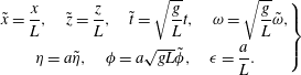 $$\begin{eqnarray}\left.\begin{array}{@{}c@{}}\tilde{x}={\displaystyle \frac{x}{L}},\quad \tilde{z}={\displaystyle \frac{z}{L}},\quad \tilde{t}=\sqrt{{\displaystyle \frac{g}{L}}}t,\quad \unicode[STIX]{x1D714}=\sqrt{{\displaystyle \frac{g}{L}}}\tilde{\unicode[STIX]{x1D714}},\\ \unicode[STIX]{x1D702}=a\tilde{\unicode[STIX]{x1D702}},\quad \unicode[STIX]{x1D719}=a\sqrt{gL}\tilde{\unicode[STIX]{x1D719}},\quad \unicode[STIX]{x1D716}={\displaystyle \frac{a}{L}}.\end{array}\right\}\end{eqnarray}$$
By following the AFM approach described in Ablowitz et al. (Reference Ablowitz, Fokas and Musslimani2006), Ashton & Fokas (Reference Ashton and Fokas2011) and dropping the tildes, the kinematic boundary condition, equation (2.2), can be written in terms of surface variables alone via the integro-differential equation
 $$\begin{eqnarray}\int _{\mathbb{R}}\,\text{d}x\text{e}^{-\text{i}kx}\text{e}^{\unicode[STIX]{x1D716}|k|\unicode[STIX]{x1D702}}(\unicode[STIX]{x1D702}_{t}+\unicode[STIX]{x1D716}\unicode[STIX]{x1D714}\unicode[STIX]{x1D702}\unicode[STIX]{x1D702}_{x}+\text{i}\text{sgn}(k)Q)=0,\quad k\neq 0,\end{eqnarray}$$
where
 $Q=q_{x}$
,
 $q(x,t)=\unicode[STIX]{x1D719}(x,\unicode[STIX]{x1D702}(x,t),t)$
. By integrating over
 $\mathbb{R}$
, we are assuming that both
 $\unicode[STIX]{x1D702}$
and
 $Q$
decay to zero sufficiently rapidly in the far field. We can also readily derive a nearly identical expression on domains periodic in the horizontal variable
 $x$
, in which case (2.5) becomes
 $$\begin{eqnarray}\int _{-L_{p}/2}^{L_{p}/2}\,\text{d}x\text{e}^{-\text{i}kx}\text{e}^{\unicode[STIX]{x1D716}|k|\unicode[STIX]{x1D702}}(\unicode[STIX]{x1D702}_{t}+\unicode[STIX]{x1D716}\unicode[STIX]{x1D714}\unicode[STIX]{x1D702}\unicode[STIX]{x1D702}_{x}+\text{i}\text{sgn}(k)Q)=0,\quad k=\frac{2\unicode[STIX]{x03C0}m}{L_{p}},m\in \mathbb{Z}\backslash 0,\end{eqnarray}$$
where
 $L_{p}$
is the spatial period. Throughout the remainder of this section we only present results over the real line,
 $\mathbb{R}$
, since identical results can be derived for the periodic case. Lastly, we note that if in (2.5) we approach
 $k=0$
from both the left and the right, we get the equations
 $$\begin{eqnarray}\int _{\mathbb{R}}\,\text{d}x(\unicode[STIX]{x1D702}_{t}+\text{i}Q)=0,\quad \int _{\mathbb{R}}\,\text{d}x(\unicode[STIX]{x1D702}_{t}-\text{i}Q)=0.\end{eqnarray}$$
Thus we get the identities
 $$\begin{eqnarray}\displaystyle & \displaystyle \unicode[STIX]{x2202}_{t}\int _{\mathbb{R}}\,\text{d}x\unicode[STIX]{x1D702}(x,t)=0, & \displaystyle\end{eqnarray}$$
 $$\begin{eqnarray}\displaystyle & \displaystyle \int _{\mathbb{R}}\,\text{d}xQ(x,t)=0. & \displaystyle\end{eqnarray}$$
Taylor expanding equation (2.5) up to
 $O(\unicode[STIX]{x1D716}^{3})$
for
 $k\neq 0$
gives
 $$\begin{eqnarray}\displaystyle & & \displaystyle \int _{\mathbb{R}}\,\text{d}x\text{e}^{-\text{i}kx}\left(1+\unicode[STIX]{x1D716}|k|\unicode[STIX]{x1D702}+\frac{\unicode[STIX]{x1D716}^{2}|k|^{2}\unicode[STIX]{x1D702}^{2}}{2}+\frac{\unicode[STIX]{x1D716}^{3}|k|^{3}\unicode[STIX]{x1D702}^{3}}{6}\right)(\unicode[STIX]{x1D702}_{t}+\text{i}\text{sgn}(k)Q)\nonumber\\ \displaystyle & & \displaystyle \quad +\,\unicode[STIX]{x1D716}\unicode[STIX]{x1D714}\int _{\mathbb{R}}\,\text{d}x\text{e}^{-\text{i}kx}\left(1+\unicode[STIX]{x1D716}|k|\unicode[STIX]{x1D702}+\frac{\unicode[STIX]{x1D716}^{2}|k|^{2}\unicode[STIX]{x1D702}^{2}}{2}\right)\unicode[STIX]{x1D702}\unicode[STIX]{x1D702}_{x}=0.\end{eqnarray}$$
Transforming into surface variables and Taylor expanding equation (2.3), Bernoulli’s equation, up to
 $O(\unicode[STIX]{x1D716}^{3})$
gives
 $$\begin{eqnarray}\displaystyle & & \displaystyle Q_{t}+\unicode[STIX]{x1D714}\unicode[STIX]{x1D702}_{t}+\unicode[STIX]{x1D702}_{x}-\tilde{\unicode[STIX]{x1D70E}}\unicode[STIX]{x1D702}_{xxx}+\frac{\unicode[STIX]{x1D716}}{2}\unicode[STIX]{x2202}_{x}(-\unicode[STIX]{x1D702}_{t}^{2}+(Q+\unicode[STIX]{x1D714}\unicode[STIX]{x1D702})^{2})\nonumber\\ \displaystyle & & \displaystyle \quad +\,\unicode[STIX]{x1D716}^{2}\unicode[STIX]{x2202}_{x}\left(\frac{3}{2}\tilde{\unicode[STIX]{x1D70E}}\unicode[STIX]{x1D702}_{x}^{2}\unicode[STIX]{x1D702}_{xx}-\unicode[STIX]{x1D702}_{t}\unicode[STIX]{x1D702}_{x}(Q+\unicode[STIX]{x1D714}\unicode[STIX]{x1D702})\right)-\frac{\unicode[STIX]{x1D716}^{3}}{2}\unicode[STIX]{x1D702}_{x}^{2}((\unicode[STIX]{x1D714}\unicode[STIX]{x1D702}+Q)^{2}-\unicode[STIX]{x1D702}_{t}^{2})=0,\end{eqnarray}$$
where the reciprocal of the Bond number,
 $\tilde{\unicode[STIX]{x1D70E}}$
, is given by
 $$\begin{eqnarray}\tilde{\unicode[STIX]{x1D70E}}=\frac{\unicode[STIX]{x1D70E}}{\unicode[STIX]{x1D70C}gL^{2}}.\end{eqnarray}$$
We note that we have tacitly assumed
 $\unicode[STIX]{x1D714}=O(1)$
. In physical terms, this implies that
 $\unicode[STIX]{x1D714}$
is comparable to the natural time scale of this problem,
 $\sqrt{L/g}$
. If we were to assume
 $\unicode[STIX]{x1D714}$
were of larger magnitude, the problem would no longer be weakly nonlinear and would be much less amenable to asymptotic analysis. Therefore, throughout the remainder of the paper, we assume that the vorticity is not too large.
The non-locality in the full equations comes from the Hilbert transform,
 ${\mathcal{H}}$
, defined by
 $$\begin{eqnarray}{\mathcal{H}}f=\frac{1}{2\unicode[STIX]{x03C0}}\int _{\mathbb{R}}\,\text{d}k\text{e}^{\text{i}kx}\text{i}\text{sgn}(k)\hat{f}(k),\end{eqnarray}$$
where
 $\hat{f}(k)$
is the Fourier transform of
 $f(x)$
defined by
 $$\begin{eqnarray}\hat{f}(k)=\int _{\mathbb{R}}\,\text{d}x~\text{e}^{-\text{i}kx}f(x).\end{eqnarray}$$
In other words,
 ${\mathcal{H}}$
is the operator with symbol
 $\text{i}\text{sgn}(k)$
. Given that
 $$\begin{eqnarray}\text{sgn}(k_{0}+\unicode[STIX]{x1D716}k)=\text{sgn}(k_{0})\text{sgn}\left(1+\frac{\unicode[STIX]{x1D716}k}{k_{0}}\right),\end{eqnarray}$$
assuming
 $\hat{f}(k)$
is a function of rapid decay, see Folland (Reference Folland1999), and assuming
 $k_{0}\gg \unicode[STIX]{x1D716}$
gives
 $$\begin{eqnarray}\displaystyle {\mathcal{H}}(f(\unicode[STIX]{x1D716}x)\text{e}^{\text{i}k_{0}x}) & = & \displaystyle \frac{\text{e}^{\text{i}k_{0}x}}{2\unicode[STIX]{x03C0}}\int _{\mathbb{R}}\,\text{d}k\text{e}^{\text{i}k\unicode[STIX]{x1D716}x}\text{i}\text{sgn}(k_{0}+\unicode[STIX]{x1D716}k)\hat{f}(k)\nonumber\\ \displaystyle & {\sim} & \displaystyle \text{i}\text{sgn}(k_{0})\text{e}^{\text{i}k_{0}x}f(\unicode[STIX]{x1D716}x),\end{eqnarray}$$
with the difference being exponentially small. On the other hand, if
 $k_{0}=0$
, then
 $$\begin{eqnarray}{\mathcal{H}}(f(\unicode[STIX]{x1D716}x))=\frac{1}{2\unicode[STIX]{x03C0}}\int _{\mathbb{R}}\,\text{d}k\text{e}^{\text{i}k\unicode[STIX]{x1D716}x}\text{i}\text{sgn}(k)\hat{f}(k)=({\mathcal{H}}f)(\unicode[STIX]{x1D716}x).\end{eqnarray}$$
Thus, the Hilbert transform does not have any significant effect on the multiple scale ansatz made below.
Equation (2.10) readily leads to a recursive formula for the surface velocity potential,
 $Q$
, of the form
 $$\begin{eqnarray}Q={\mathcal{H}}\unicode[STIX]{x2202}_{t}\unicode[STIX]{x1D702}+\unicode[STIX]{x1D716}R_{1}+\unicode[STIX]{x1D716}^{2}R_{2}+\unicode[STIX]{x1D716}^{3}R_{3},\end{eqnarray}$$
where
 $$\begin{eqnarray}\left.\begin{array}{@{}c@{}}R_{1}={\mathcal{H}}\unicode[STIX]{x2202}_{x}\left(\unicode[STIX]{x1D702}{\mathcal{H}}\unicode[STIX]{x2202}_{t}\unicode[STIX]{x1D702}+{\displaystyle \frac{\unicode[STIX]{x1D714}}{2}}\unicode[STIX]{x1D702}^{2}-{\displaystyle \frac{1}{2}}{\mathcal{H}}\unicode[STIX]{x2202}_{t}\unicode[STIX]{x1D702}^{2}\right),\\ R_{2}={\mathcal{H}}\unicode[STIX]{x2202}_{x}\left(\unicode[STIX]{x1D702}R_{1}\right)-{\mathcal{H}}\unicode[STIX]{x2202}_{x}^{2}\left({\displaystyle \frac{1}{6}}\unicode[STIX]{x2202}_{t}\unicode[STIX]{x1D702}^{3}+{\displaystyle \frac{\unicode[STIX]{x1D714}}{3}}{\mathcal{H}}\unicode[STIX]{x1D702}^{3}+{\displaystyle \frac{1}{2}}{\mathcal{H}}(\unicode[STIX]{x1D702}^{2}{\mathcal{H}}\unicode[STIX]{x2202}_{t}\unicode[STIX]{x1D702})\right),\\ R_{3}={\mathcal{H}}\unicode[STIX]{x2202}_{x}\left(\unicode[STIX]{x1D702}R_{2}\right)+{\displaystyle \frac{1}{2}}\unicode[STIX]{x2202}_{x}^{2}\left(\unicode[STIX]{x1D702}^{2}R_{1}\right)+{\mathcal{H}}\unicode[STIX]{x2202}_{x}^{3}\left({\displaystyle \frac{1}{24}}{\mathcal{H}}\unicode[STIX]{x2202}_{t}\unicode[STIX]{x1D702}^{4}-{\displaystyle \frac{1}{6}}\unicode[STIX]{x1D702}^{3}{\mathcal{H}}\unicode[STIX]{x2202}_{t}\unicode[STIX]{x1D702}-{\displaystyle \frac{\unicode[STIX]{x1D714}}{8}}\unicode[STIX]{x1D702}^{4}\right).\end{array}\right\}\end{eqnarray}$$
Coupling this to (2.11) gives a single scalar equation defined entirely in terms of the surface height,
 $\unicode[STIX]{x1D702}$
. Now, use the ansatz
 $$\begin{eqnarray}\displaystyle \unicode[STIX]{x1D702}(x,t) & = & \displaystyle \unicode[STIX]{x1D716}\unicode[STIX]{x1D702}_{0}(\unicode[STIX]{x1D709},\unicode[STIX]{x1D70F})+\unicode[STIX]{x1D702}_{1}(\unicode[STIX]{x1D709},\unicode[STIX]{x1D70F})\text{e}^{\text{i}\unicode[STIX]{x1D703}}+\unicode[STIX]{x1D702}_{1}^{\ast }(\unicode[STIX]{x1D709},\unicode[STIX]{x1D70F})\text{e}^{-\text{i}\unicode[STIX]{x1D703}}+\unicode[STIX]{x1D716}(\unicode[STIX]{x1D702}_{2}(\unicode[STIX]{x1D709},\unicode[STIX]{x1D70F})\text{e}^{2\text{i}\unicode[STIX]{x1D703}}+\unicode[STIX]{x1D702}_{2}^{\ast }(\unicode[STIX]{x1D709},\unicode[STIX]{x1D70F})\text{e}^{-2\text{i}\unicode[STIX]{x1D703}})\nonumber\\ \displaystyle & & \displaystyle +\,\unicode[STIX]{x1D716}^{2}(\unicode[STIX]{x1D702}_{3}(\unicode[STIX]{x1D709},\unicode[STIX]{x1D70F})e^{3i\unicode[STIX]{x1D703}}+\unicode[STIX]{x1D702}_{3}^{\ast }(\unicode[STIX]{x1D709},\unicode[STIX]{x1D70F})e^{-3i\unicode[STIX]{x1D703}})+\unicode[STIX]{x1D716}^{3}(\unicode[STIX]{x1D702}_{4}(\unicode[STIX]{x1D709},\unicode[STIX]{x1D70F})e^{4i\unicode[STIX]{x1D703}}+\unicode[STIX]{x1D702}_{4}^{\ast }(\unicode[STIX]{x1D709},\unicode[STIX]{x1D70F})e^{-4i\unicode[STIX]{x1D703}})+\cdots \,,\nonumber\\ \displaystyle & & \displaystyle\end{eqnarray}$$
where
 $$\begin{eqnarray}\unicode[STIX]{x1D703}=k_{0}x+\unicode[STIX]{x1D6FA}t,\quad \unicode[STIX]{x1D709}=\unicode[STIX]{x1D716}(x+c_{g}t),\quad \unicode[STIX]{x1D70F}=\unicode[STIX]{x1D716}^{2}t.\end{eqnarray}$$
We note that using integration by parts shows that terms of the form
 $\unicode[STIX]{x1D702}_{m}\text{e}^{\text{i}m\unicode[STIX]{x1D703}}$
satisfy
 $$\begin{eqnarray}\int _{\mathbb{R}}\,\text{d}x\unicode[STIX]{x1D702}_{m}(\unicode[STIX]{x1D709},\unicode[STIX]{x1D70F})\text{e}^{\text{i}m\unicode[STIX]{x1D703}}=O(\unicode[STIX]{x1D716}^{j}),\quad j\geqslant 1,m>0,\end{eqnarray}$$
which is to say that these terms are vanishingly small in an asymptotic sense. Thus, asymptotically, equation (2.8) becomes
 $$\begin{eqnarray}\unicode[STIX]{x2202}_{\unicode[STIX]{x1D70F}}\int _{\mathbb{R}}\,\text{d}\unicode[STIX]{x1D709}\unicode[STIX]{x1D702}_{0}(\unicode[STIX]{x1D709},\unicode[STIX]{x1D70F})=0.\end{eqnarray}$$
By expanding and matching terms in the fundamental harmonic,
 $\text{e}^{\text{i}\unicode[STIX]{x1D703}}$
, at
 $O(1)$
we obtain the linear dispersion relation,
 $$\begin{eqnarray}\unicode[STIX]{x1D6FA}_{\pm }(k_{0},\unicode[STIX]{x1D714})=\frac{1}{2}\left(s\unicode[STIX]{x1D714}\pm \sqrt{\unicode[STIX]{x1D714}^{2}+4|k_{0}|(1+\tilde{\unicode[STIX]{x1D70E}}k_{0}^{2})}\right),\end{eqnarray}$$
and at
 $O(\unicode[STIX]{x1D716})$
we find that
 $$\begin{eqnarray}c_{g}=\frac{1+3\tilde{\unicode[STIX]{x1D70E}}k_{0}^{2}}{2s\unicode[STIX]{x1D6FA}-\unicode[STIX]{x1D714}},\end{eqnarray}$$
where
 $s=\text{sgn}(k_{0})$
. We note that (2.24) establishes that
 $\unicode[STIX]{x1D6FA}_{+}(k_{0},\unicode[STIX]{x1D714})>0$
and
 $\unicode[STIX]{x1D6FA}_{-}(k_{0},\unicode[STIX]{x1D714})<0$
for
 $k_{0}\neq 0$
. Throughout the remainder of the paper,
 $\unicode[STIX]{x1D6FA}$
always denotes the positive branch,
 $\unicode[STIX]{x1D6FA}_{+}$
. By looking at the second harmonic,
 $\text{e}^{2\text{i}\unicode[STIX]{x1D703}}$
, we find that
 $$\begin{eqnarray}\unicode[STIX]{x1D702}_{2}=\ell _{0}\unicode[STIX]{x1D702}_{1}^{2}+\text{i}\unicode[STIX]{x1D716}\ell _{1}\unicode[STIX]{x1D702}_{1}\unicode[STIX]{x2202}_{\unicode[STIX]{x1D709}}\unicode[STIX]{x1D702}_{1}+O(\unicode[STIX]{x1D716}^{2}),\end{eqnarray}$$
where
 $$\begin{eqnarray}\left.\begin{array}{@{}c@{}}\ell _{0}=-{\displaystyle \frac{k_{0}(\unicode[STIX]{x1D714}^{2}+2\unicode[STIX]{x1D6FA}^{2}-4s\unicode[STIX]{x1D714}\unicode[STIX]{x1D6FA})}{2(k_{0}+\unicode[STIX]{x1D714}\unicode[STIX]{x1D6FA}-2s\unicode[STIX]{x1D6FA}^{2}+4\tilde{\unicode[STIX]{x1D70E}}k_{0}^{3})}},\\ \ell _{1}={\displaystyle \frac{(2c_{g}k_{0}(\unicode[STIX]{x1D6FA}-s\unicode[STIX]{x1D714})-2s\unicode[STIX]{x1D714}\unicode[STIX]{x1D6FA}+\unicode[STIX]{x1D6FA}^{2}+\unicode[STIX]{x1D714}^{2}/2)+(1+\unicode[STIX]{x1D714}c_{g}+12k_{0}^{2}\tilde{\unicode[STIX]{x1D70E}}-4sc_{g}\unicode[STIX]{x1D6FA})\ell _{0}}{k_{0}+\unicode[STIX]{x1D714}\unicode[STIX]{x1D6FA}-2s\unicode[STIX]{x1D6FA}^{2}+4\tilde{\unicode[STIX]{x1D70E}}k_{0}^{3}}}.\end{array}\right\}\end{eqnarray}$$
By then going up to
 $O(\unicode[STIX]{x1D716}^{3})$
, we get the following coupled system describing the slow spatial and temporal modulation due to the interaction of the leading harmonic term,
 $\unicode[STIX]{x1D702}_{1}$
, and the mean surface height,
 $\unicode[STIX]{x1D702}_{0}$
,
 $$\begin{eqnarray}\displaystyle & & \displaystyle \unicode[STIX]{x1D716}c_{g}^{2}{\mathcal{H}}\unicode[STIX]{x2202}_{\unicode[STIX]{x1D709}}^{2}\unicode[STIX]{x1D702}_{0}+(1+\unicode[STIX]{x1D714}c_{g})\unicode[STIX]{x2202}_{\unicode[STIX]{x1D709}}\unicode[STIX]{x1D702}_{0}+\unicode[STIX]{x1D716}\unicode[STIX]{x1D714}\unicode[STIX]{x2202}_{\unicode[STIX]{x1D70F}}\unicode[STIX]{x1D702}_{0}+\unicode[STIX]{x1D714}(\unicode[STIX]{x1D714}-2s\unicode[STIX]{x1D6FA})\unicode[STIX]{x2202}_{\unicode[STIX]{x1D709}}|\unicode[STIX]{x1D702}_{1}|^{2}\nonumber\\ \displaystyle & & \displaystyle \quad +\,\unicode[STIX]{x1D716}(c_{g}(\unicode[STIX]{x1D714}-2s\unicode[STIX]{x1D6FA}){\mathcal{H}}\unicode[STIX]{x2202}_{\unicode[STIX]{x1D709}}^{2}|\unicode[STIX]{x1D702}_{1}|^{2}+\text{i}s\unicode[STIX]{x1D714}c_{g}(\unicode[STIX]{x1D702}_{1}^{\ast }\unicode[STIX]{x2202}_{\unicode[STIX]{x1D709}}^{2}\unicode[STIX]{x1D702}_{1}-\unicode[STIX]{x1D702}_{1}\unicode[STIX]{x2202}_{\unicode[STIX]{x1D709}}^{2}\unicode[STIX]{x1D702}_{1}^{\ast }))=0,\end{eqnarray}$$
 $$\begin{eqnarray}\displaystyle & & \displaystyle (\unicode[STIX]{x1D714}-2s\unicode[STIX]{x1D6FA})\unicode[STIX]{x2202}_{\unicode[STIX]{x1D70F}}\unicode[STIX]{x1D702}_{1}+\text{i}(c_{g}^{2}s-3k_{0}\tilde{\unicode[STIX]{x1D70E}})\unicode[STIX]{x2202}_{\unicode[STIX]{x1D709}}^{2}\unicode[STIX]{x1D702}_{1}+2\text{i}\unicode[STIX]{x1D716}sc_{g}\unicode[STIX]{x2202}_{\unicode[STIX]{x1D709}\unicode[STIX]{x1D70F}}^{2}\unicode[STIX]{x1D702}_{1}-\unicode[STIX]{x1D716}\tilde{\unicode[STIX]{x1D70E}}\unicode[STIX]{x2202}_{\unicode[STIX]{x1D709}}^{3}\unicode[STIX]{x1D702}_{1}\nonumber\\ \displaystyle & & \displaystyle \qquad +\,\text{i}k_{0}\unicode[STIX]{x1D714}(\unicode[STIX]{x1D714}-2s\unicode[STIX]{x1D6FA})\unicode[STIX]{x1D702}_{0}\unicode[STIX]{x1D702}_{1}+\text{i}\unicode[STIX]{x1D6FC}_{0}|\unicode[STIX]{x1D702}_{1}|^{2}\unicode[STIX]{x1D702}_{1}+\unicode[STIX]{x1D716}\unicode[STIX]{x1D6FC}_{1}|\unicode[STIX]{x1D702}_{1}|^{2}\unicode[STIX]{x2202}_{\unicode[STIX]{x1D709}}\unicode[STIX]{x1D702}_{1}+\unicode[STIX]{x1D716}\unicode[STIX]{x1D6FC}_{2}\unicode[STIX]{x1D702}_{1}^{2}\unicode[STIX]{x2202}_{\unicode[STIX]{x1D709}}\unicode[STIX]{x1D702}_{1}^{\ast }+\nonumber\\ \displaystyle & & \displaystyle \quad \unicode[STIX]{x1D716}\text{i}\unicode[STIX]{x1D6FC}_{3}\unicode[STIX]{x1D702}_{1}{\mathcal{H}}\unicode[STIX]{x2202}_{\unicode[STIX]{x1D709}}|\unicode[STIX]{x1D702}_{1}|^{2}+\unicode[STIX]{x1D716}\unicode[STIX]{x1D714}(\unicode[STIX]{x1D714}-2s\unicode[STIX]{x1D6FA}-|k_{0}|c_{g})\unicode[STIX]{x1D702}_{1}\unicode[STIX]{x2202}_{\unicode[STIX]{x1D709}}\unicode[STIX]{x1D702}_{0}+\unicode[STIX]{x1D716}\unicode[STIX]{x1D714}(\unicode[STIX]{x1D714}-2s\unicode[STIX]{x1D6FA}-2|k_{0}|c_{g})\unicode[STIX]{x1D702}_{0}\unicode[STIX]{x2202}_{\unicode[STIX]{x1D709}}\unicode[STIX]{x1D702}_{1}\nonumber\\ \displaystyle & & \displaystyle \qquad +\,\unicode[STIX]{x1D716}\text{i}k_{0}c_{g}(\unicode[STIX]{x1D714}-2s\unicode[STIX]{x1D6FA})\unicode[STIX]{x1D702}_{1}{\mathcal{H}}\unicode[STIX]{x2202}_{\unicode[STIX]{x1D709}}\unicode[STIX]{x1D702}_{0}=0,\end{eqnarray}$$
where
 $$\begin{eqnarray}\left.\begin{array}{@{}c@{}}\unicode[STIX]{x1D6FC}_{0}=k_{0}^{2}\left(-{\textstyle \frac{3}{2}}k_{0}^{3}\tilde{\unicode[STIX]{x1D70E}}+2s\unicode[STIX]{x1D6FA}^{2}-s\unicode[STIX]{x1D714}^{2}\right)+\ell _{0}k_{0}(\unicode[STIX]{x1D714}^{2}+2\unicode[STIX]{x1D6FA}^{2}-4s\unicode[STIX]{x1D714}\unicode[STIX]{x1D6FA}),\\ \unicode[STIX]{x1D6FC}_{1}=k_{0}(4c_{g}|k_{0}|\unicode[STIX]{x1D6FA}-9\tilde{\unicode[STIX]{x1D70E}}k_{0}^{3}+6s\unicode[STIX]{x1D6FA}^{2}-3s\unicode[STIX]{x1D714}^{2})+\ell _{0} (\!2\unicode[STIX]{x1D714}^{2}+4\unicode[STIX]{x1D6FA}^{2}\\ \qquad -\,8s\unicode[STIX]{x1D714}\unicode[STIX]{x1D6FA}+4k_{0}c_{g}(\unicode[STIX]{x1D6FA}-s\unicode[STIX]{x1D714})\!)+\ell _{1}k_{0}(4s\unicode[STIX]{x1D714}\unicode[STIX]{x1D6FA}-2\unicode[STIX]{x1D6FA}^{2}-\unicode[STIX]{x1D714}^{2}),\\ \unicode[STIX]{x1D6FC}_{2}=k_{0}\left(-{\textstyle \frac{3}{2}}k_{0}^{3}\tilde{\unicode[STIX]{x1D70E}}+2s\unicode[STIX]{x1D6FA}^{2}-s\unicode[STIX]{x1D714}^{2}\right)+\ell _{0}(\unicode[STIX]{x1D714}^{2}+2\unicode[STIX]{x1D6FA}^{2}-4s\unicode[STIX]{x1D714}\unicode[STIX]{x1D6FA}),\\ \unicode[STIX]{x1D6FC}_{3}=k_{0}(\unicode[STIX]{x1D714}-2s\unicode[STIX]{x1D6FA})^{2}.\end{array}\right\}\end{eqnarray}$$
By solving (2.28) to leading order and using (2.23), we find that
 $$\begin{eqnarray}\unicode[STIX]{x1D702}_{0}(\unicode[STIX]{x1D709},\unicode[STIX]{x1D70F})=\frac{\unicode[STIX]{x1D714}(2s\unicode[STIX]{x1D6FA}-\unicode[STIX]{x1D714})}{1+\unicode[STIX]{x1D714}c_{g}}|\unicode[STIX]{x1D702}_{1}|^{2}(\unicode[STIX]{x1D709},\unicode[STIX]{x1D70F})+O(\unicode[STIX]{x1D716}).\end{eqnarray}$$
Likewise, from (2.29) at this order, and using the leading-order solution for the mean height,
 $\unicode[STIX]{x1D702}_{0}$
, gives the time-dependent NLS equation
 $$\begin{eqnarray}\text{i}\unicode[STIX]{x2202}_{\unicode[STIX]{x1D70F}}\unicode[STIX]{x1D702}_{1}+\unicode[STIX]{x1D6FC}_{nl}|\unicode[STIX]{x1D702}_{1}|^{2}\unicode[STIX]{x1D702}_{1}+\unicode[STIX]{x1D6FC}_{d}\unicode[STIX]{x2202}_{\unicode[STIX]{x1D709}}^{2}\unicode[STIX]{x1D702}_{1}=0,\end{eqnarray}$$
where
 $$\begin{eqnarray}\left.\begin{array}{@{}c@{}}\unicode[STIX]{x1D6FC}_{d}(k_{0},\unicode[STIX]{x1D714})={\displaystyle \frac{(c_{g}^{2}-3|k_{0}|\tilde{\unicode[STIX]{x1D70E}})}{2\unicode[STIX]{x1D6FA}-s\unicode[STIX]{x1D714}}},\\ \unicode[STIX]{x1D6FC}_{nl}(k_{0},\unicode[STIX]{x1D714})={\displaystyle \frac{k_{0}(sk_{0}^{3}(8+\tilde{\unicode[STIX]{x1D70E}}k_{0}^{2}+2(\tilde{\unicode[STIX]{x1D70E}}k_{0}^{2})^{2})+\unicode[STIX]{x1D714}\unicode[STIX]{x1D6FC}_{v})}{(2s\unicode[STIX]{x1D6FA}-\unicode[STIX]{x1D714})(1+c_{g}\unicode[STIX]{x1D714})(4\unicode[STIX]{x1D6FA}^{2}-s(2k_{0}(1+4\tilde{\unicode[STIX]{x1D70E}}k_{0}^{2})+2\unicode[STIX]{x1D714}\unicode[STIX]{x1D6FA}))}},\end{array}\right\}\end{eqnarray}$$
and
 $$\begin{eqnarray}\displaystyle \unicode[STIX]{x1D6FC}_{v}(k_{0},\unicode[STIX]{x1D714}) & = & \displaystyle s(c_{g}k_{0}-2\unicode[STIX]{x1D6FA})\unicode[STIX]{x1D714}^{4}+k_{0}(4k_{0}^{2}s\tilde{\unicode[STIX]{x1D70E}}+2\unicode[STIX]{x1D6FA}c_{g}-s)\unicode[STIX]{x1D714}^{3}\nonumber\\ \displaystyle & & \displaystyle +\,k_{0}(16c_{g}k_{0}^{3}\tilde{\unicode[STIX]{x1D70E}}-8\unicode[STIX]{x1D6FA}k_{0}^{2}\tilde{\unicode[STIX]{x1D70E}}+10c_{g}k_{0}-6\unicode[STIX]{x1D6FA})\unicode[STIX]{x1D714}^{2}\nonumber\\ \displaystyle & & \displaystyle -\,k_{0}^{2}(15\unicode[STIX]{x1D6FA}c_{g}k_{0}^{2}s\tilde{\unicode[STIX]{x1D70E}}-16k_{0}^{4}\tilde{\unicode[STIX]{x1D70E}}^{2}-24k_{0}^{2}\tilde{\unicode[STIX]{x1D70E}}-2)\unicode[STIX]{x1D714}\nonumber\\ \displaystyle & & \displaystyle +\,k_{0}^{3}(2c_{g}k_{0}^{4}s\tilde{\unicode[STIX]{x1D70E}}^{2}+c_{g}k_{0}^{2}s\tilde{\unicode[STIX]{x1D70E}}-15\unicode[STIX]{x1D6FA}k_{0}s\tilde{\unicode[STIX]{x1D70E}}+8c_{g}s).\end{eqnarray}$$
Note, our results for the NLS equation agree with those in Ablowitz et al. (Reference Ablowitz, Fokas and Musslimani2006) for
 $\unicode[STIX]{x1D714}=0$
, and they agree with the results in Thomas et al. (Reference Thomas, Kharif and Manna2012) for
 $\tilde{\unicode[STIX]{x1D70E}}=0$
. Further, all of our results in this section are derived with the aid of the computer algebra system SAGE.
We readily see that we can go to higher order in the mean term using (2.28) and the expansion
 $$\begin{eqnarray}\unicode[STIX]{x1D702}_{0}(\unicode[STIX]{x1D709},\unicode[STIX]{x1D70F})=\frac{\unicode[STIX]{x1D714}(2s\unicode[STIX]{x1D6FA}-\unicode[STIX]{x1D714})}{1+\unicode[STIX]{x1D714}c_{g}}|\unicode[STIX]{x1D702}_{1}|^{2}(\unicode[STIX]{x1D709},\unicode[STIX]{x1D70F})+\unicode[STIX]{x1D716}\unicode[STIX]{x1D702}_{01}(\unicode[STIX]{x1D709},\unicode[STIX]{x1D70F})+O(\unicode[STIX]{x1D716}^{2}),\end{eqnarray}$$
which gives
 $$\begin{eqnarray}\unicode[STIX]{x1D702}_{01}=\frac{c_{g}(2s\unicode[STIX]{x1D6FA}-\unicode[STIX]{x1D714})}{(1+\unicode[STIX]{x1D714}c_{g})^{2}}{\mathcal{H}}\unicode[STIX]{x2202}_{\unicode[STIX]{x1D709}}|\unicode[STIX]{x1D702}_{1}|^{2}+\frac{\text{i}\unicode[STIX]{x1D714}}{1+\unicode[STIX]{x1D714}c_{g}}\left(\frac{\unicode[STIX]{x1D6FC}_{d}\unicode[STIX]{x1D714}(2s\unicode[STIX]{x1D6FA}-\unicode[STIX]{x1D714})}{1+\unicode[STIX]{x1D714}c_{g}}+sc_{g}\right)(\unicode[STIX]{x1D702}_{1}\unicode[STIX]{x2202}_{\unicode[STIX]{x1D709}}\unicode[STIX]{x1D702}_{1}^{\ast }-\unicode[STIX]{x1D702}_{1}^{\ast }\unicode[STIX]{x2202}_{\unicode[STIX]{x1D709}}\unicode[STIX]{x1D702}_{1}).\end{eqnarray}$$
Thus, equation (2.29) can be written in terms of
 $\unicode[STIX]{x1D702}_{1}$
alone
 $$\begin{eqnarray}\displaystyle & & \displaystyle (\unicode[STIX]{x1D714}-2s\unicode[STIX]{x1D6FA})\unicode[STIX]{x2202}_{\unicode[STIX]{x1D70F}}\unicode[STIX]{x1D702}_{1}+\text{i}(c_{g}^{2}s-3k_{0}\tilde{\unicode[STIX]{x1D70E}})\unicode[STIX]{x2202}_{\unicode[STIX]{x1D709}}^{2}\unicode[STIX]{x1D702}_{1}+2\text{i}\unicode[STIX]{x1D716}sc_{g}\unicode[STIX]{x2202}_{\unicode[STIX]{x1D709}\unicode[STIX]{x1D70F}}^{2}\unicode[STIX]{x1D702}_{1}-\unicode[STIX]{x1D716}\tilde{\unicode[STIX]{x1D70E}}\unicode[STIX]{x2202}_{\unicode[STIX]{x1D709}}^{3}\unicode[STIX]{x1D702}_{1}\nonumber\\ \displaystyle & & \displaystyle \quad -\,\text{i}\unicode[STIX]{x1D6FC}_{nl}(\unicode[STIX]{x1D714}-2s\unicode[STIX]{x1D6FA})|\unicode[STIX]{x1D702}_{1}|^{2}\unicode[STIX]{x1D702}_{1}+\unicode[STIX]{x1D716}\tilde{\unicode[STIX]{x1D6FC}}_{1}|\unicode[STIX]{x1D702}_{1}|^{2}\unicode[STIX]{x2202}_{\unicode[STIX]{x1D709}}\unicode[STIX]{x1D702}_{1}+\unicode[STIX]{x1D716}\tilde{\unicode[STIX]{x1D6FC}}_{2}\unicode[STIX]{x1D702}_{1}^{2}\unicode[STIX]{x2202}_{\unicode[STIX]{x1D709}}\unicode[STIX]{x1D702}_{1}^{\ast }+\unicode[STIX]{x1D716}\text{i}\tilde{\unicode[STIX]{x1D6FC}}_{3}\unicode[STIX]{x1D702}_{1}{\mathcal{H}}\unicode[STIX]{x2202}_{\unicode[STIX]{x1D709}}|\unicode[STIX]{x1D702}_{1}|^{2}=0.\qquad\end{eqnarray}$$
Obtaining the coefficients,
 $\tilde{\unicode[STIX]{x1D6FC}}_{j}$
, is straightforward, and thus we omit writing them down for the sake of brevity. We call (2.37) the VD equation. By solving it, we in effect find the next-order correction to the NLS equation, and thus, by combining with our previous results, we can find
 $\unicode[STIX]{x1D702}$
up to
 $O(\unicode[STIX]{x1D716}^{2})$
on a
 $O(1/\unicode[STIX]{x1D716}^{2})$
time scale. This becomes a critical feature necessary to ensure the accuracy of our numerics in § 4.
For the NLS equation, the case in which
 $\unicode[STIX]{x1D6FC}_{d}$
and
 $\unicode[STIX]{x1D6FC}_{nl}$
have the same sign is known as the ‘focusing’ case while the case in which they have opposite signs is known as the ‘defocusing’ case. These two cases are qualitatively different. In the focusing case, the trivial-phase Jacobi elliptic solutions are given by
 $$\begin{eqnarray}\unicode[STIX]{x1D702}_{1}(\unicode[STIX]{x1D709},\unicode[STIX]{x1D70F})=\unicode[STIX]{x1D705}\unicode[STIX]{x1D6FD}\sqrt{\frac{2\unicode[STIX]{x1D6FC}_{d}}{\unicode[STIX]{x1D6FC}_{nl}}}\text{cn}(\unicode[STIX]{x1D6FD}\unicode[STIX]{x1D709};\unicode[STIX]{x1D705})\text{e}^{-\text{i}\unicode[STIX]{x1D6FC}_{d}\unicode[STIX]{x1D6FD}^{2}(1-2\unicode[STIX]{x1D705}^{2})\unicode[STIX]{x1D70F}},\end{eqnarray}$$
where
 $0\leqslant \unicode[STIX]{x1D705}\leqslant 1$
is the elliptic modulus and
 $\unicode[STIX]{x1D6FD}$
is a positive length scale parameter. In the
 $\unicode[STIX]{x1D705}\rightarrow 1$
limit, these solutions limit to the ‘bright’-soliton solutions
 $$\begin{eqnarray}\unicode[STIX]{x1D702}_{1}(\unicode[STIX]{x1D709},\unicode[STIX]{x1D70F})=\unicode[STIX]{x1D6FD}\sqrt{\frac{2\unicode[STIX]{x1D6FC}_{d}}{\unicode[STIX]{x1D6FC}_{nl}}}\text{sech}(\unicode[STIX]{x1D6FD}\unicode[STIX]{x1D709})\text{e}^{\text{i}\unicode[STIX]{x1D6FC}_{d}\unicode[STIX]{x1D6FD}^{2}\unicode[STIX]{x1D70F}}.\end{eqnarray}$$
In the defocusing case, the trivial-phase Jacobi elliptic solutions are given by
 $$\begin{eqnarray}\unicode[STIX]{x1D702}_{1}(\unicode[STIX]{x1D709},\unicode[STIX]{x1D70F})=\unicode[STIX]{x1D705}\unicode[STIX]{x1D6FD}\sqrt{-\frac{2\unicode[STIX]{x1D6FC}_{d}}{\unicode[STIX]{x1D6FC}_{nl}}}\text{sn}(\unicode[STIX]{x1D6FD}\unicode[STIX]{x1D709};\unicode[STIX]{x1D705})\text{e}^{-\text{i}\unicode[STIX]{x1D6FC}_{d}\unicode[STIX]{x1D6FD}^{2}(1+\unicode[STIX]{x1D705}^{2})\unicode[STIX]{x1D70F}}.\end{eqnarray}$$
In the
 $\unicode[STIX]{x1D705}\rightarrow 1$
limit, these solutions limit to the ‘dark’-soliton solutions
 $$\begin{eqnarray}\unicode[STIX]{x1D702}_{1}(\unicode[STIX]{x1D709},\unicode[STIX]{x1D70F})=\unicode[STIX]{x1D6FD}\sqrt{-\frac{2\unicode[STIX]{x1D6FC}_{d}}{\unicode[STIX]{x1D6FC}_{nl}}}\text{tanh}(\unicode[STIX]{x1D6FD}\unicode[STIX]{x1D709})\text{e}^{-2\text{i}\unicode[STIX]{x1D6FC}_{d}\unicode[STIX]{x1D6FD}^{2}\unicode[STIX]{x1D70F}}.\end{eqnarray}$$
The elevated profile of the magnitude of the bright soliton is qualitatively different from the depressed profile of the magnitude of the dark soliton. This distinction typifies the difference between the behaviour of the focusing and defocusing cases. Note that in order for
 $\unicode[STIX]{x1D702}(x,t)$
to be periodic when Jacobi elliptic functions are used, the following restriction must be enforced
 $$\begin{eqnarray}k_{0}=\frac{\unicode[STIX]{x03C0}\unicode[STIX]{x1D716}m}{2K(\unicode[STIX]{x1D705})},\quad m\in \mathbb{Z},\end{eqnarray}$$
where
 $K(\unicode[STIX]{x1D705})$
is the complete elliptic integral of the first kind.
2.2 Modulational instabilities and currents in infinite depth
The plane-wave, or Stokes wave, solutions of the NLS equation are given by
 $$\begin{eqnarray}\unicode[STIX]{x1D702}_{1}(\unicode[STIX]{x1D709},\unicode[STIX]{x1D70F})=A\text{e}^{\text{i}\unicode[STIX]{x1D6FC}_{nl}A^{2}\unicode[STIX]{x1D70F}},\end{eqnarray}$$
where
 $A>0$
is a real constant. Complementing the results in Thomas et al. (Reference Thomas, Kharif and Manna2012), we study the stability of these solutions by considering perturbed solutions of the form
 $$\begin{eqnarray}\unicode[STIX]{x1D702}_{1p}(\unicode[STIX]{x1D709},\unicode[STIX]{x1D70F})=(A+\unicode[STIX]{x1D707}(u_{p}(\unicode[STIX]{x1D709},\unicode[STIX]{x1D70F})+iv_{p}(\unicode[STIX]{x1D709},\unicode[STIX]{x1D70F}))+O(\unicode[STIX]{x1D707}^{2}))\text{e}^{\text{i}\unicode[STIX]{x1D6FC}_{nl}A^{2}\unicode[STIX]{x1D70F}},\end{eqnarray}$$
where
 $\unicode[STIX]{x1D707}$
is a small real parameter and
 $u_{p}$
and
 $v_{p}$
are real-valued functions. Substituting (2.44) into the NLS equation and linearizing gives
 $$\begin{eqnarray}\unicode[STIX]{x2202}_{\unicode[STIX]{x1D70F}}\left(\begin{array}{@{}c@{}}u_{p}\\ v_{p}\end{array}\right)=\left(\begin{array}{@{}cc@{}}0 & -\unicode[STIX]{x1D6FC}_{d}\unicode[STIX]{x2202}_{\unicode[STIX]{x1D709}}^{2}\\ \unicode[STIX]{x1D6FC}_{d}\unicode[STIX]{x2202}_{\unicode[STIX]{x1D709}}^{2}+2A^{2}\unicode[STIX]{x1D6FC}_{nl} & 0\end{array}\right)\left(\begin{array}{@{}c@{}}u_{p}\\ v_{p}\end{array}\right).\end{eqnarray}$$
Separating variables, applying a Fourier transform in
 $\unicode[STIX]{x1D709}$
, and introducing the
 $\unicode[STIX]{x1D709}$
wavenumber
 $l$
, establishes that NLS plane-wave solutions are unstable with respect to the modulational instabilities (MIs) if
 $$\begin{eqnarray}0<l^{2}\leqslant 2\frac{\unicode[STIX]{x1D6FC}_{nl}}{\unicode[STIX]{x1D6FC}_{d}}A^{2}.\end{eqnarray}$$
This reduces to the classic requirement that MIs are suppressed if the coefficients of dispersion and nonlinearity have opposite signs (i.e. the defocusing case).
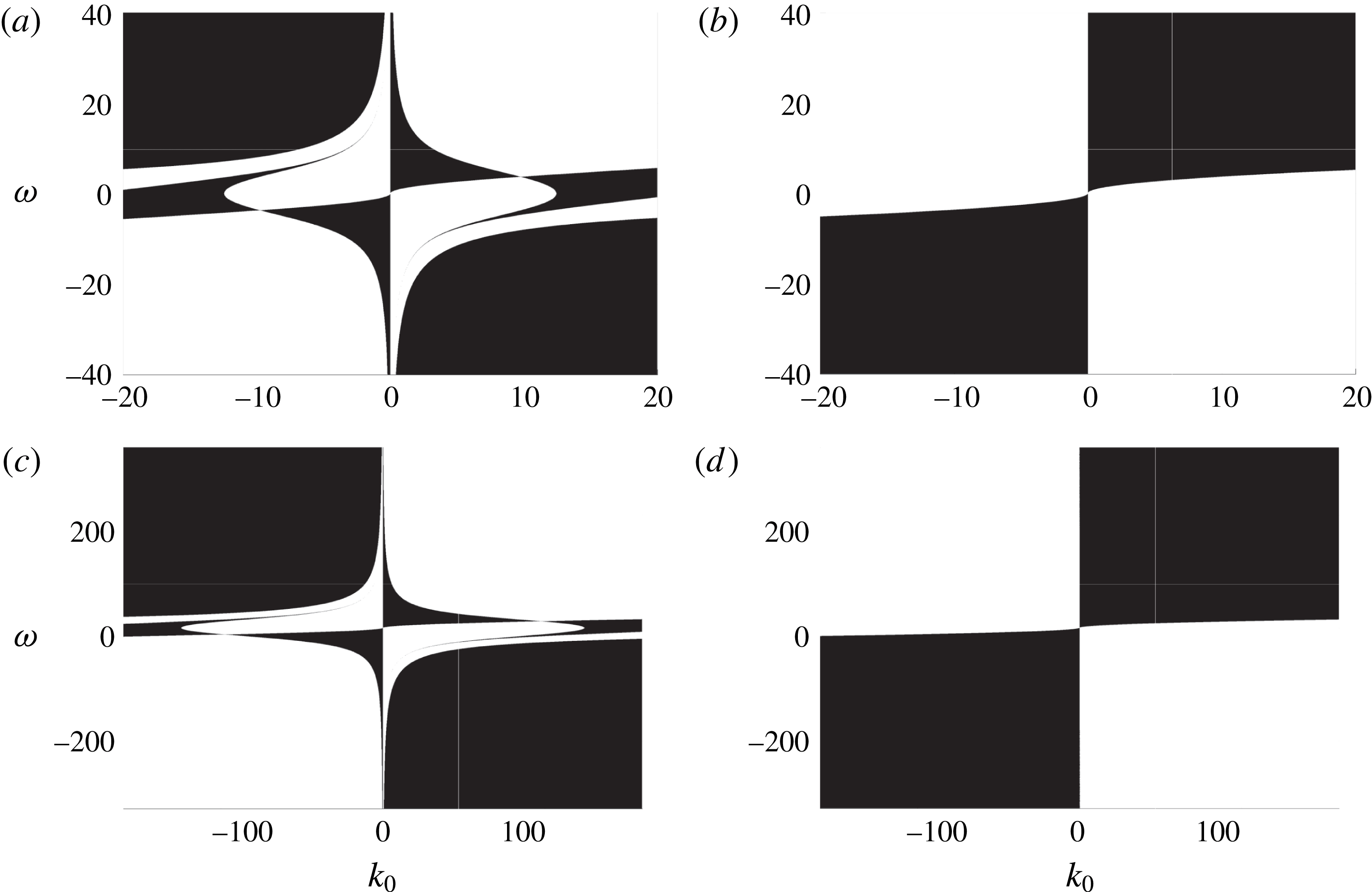
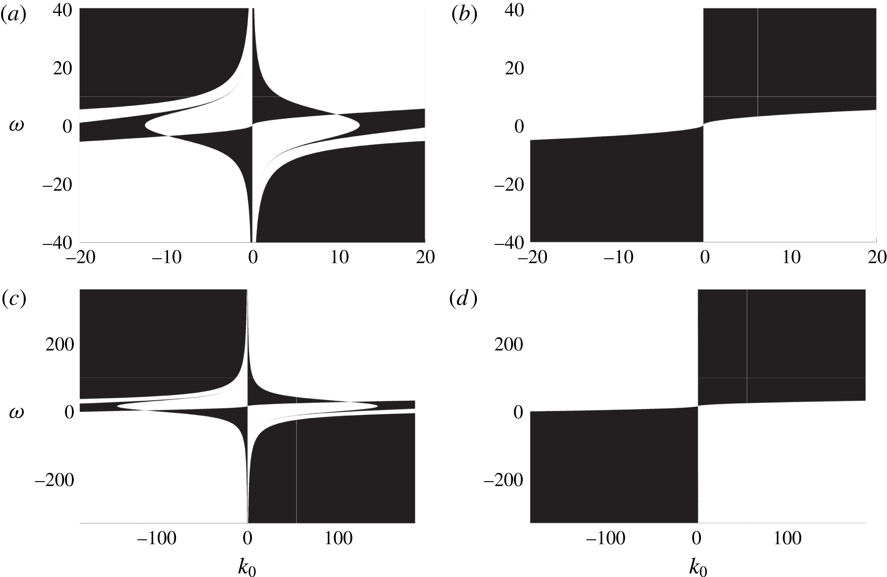
Figure 1 shows the values of
 $\unicode[STIX]{x1D714}$
and
 $k_{0}$
for which MIs exist (white areas) or not (black areas) for
 $\tilde{\unicode[STIX]{x1D70E}}=10^{-3}$
in figure 1(a),
 $\tilde{\unicode[STIX]{x1D70E}}=10^{-5}$
in figure 1(b),
 $\tilde{\unicode[STIX]{x1D70E}}=10^{-5}$
in figure 1(c) and
 $\tilde{\unicode[STIX]{x1D70E}}=0$
in figure 1(d). Note, the scale of the axes changes from figure 1(a,b) to (c,d). Further, while we assumed that
 $\unicode[STIX]{x1D714}=O(1)$
in our derivation of the NLS equation, to see the impact of surface tension and its connection to MI, we have had to plot on an exaggerated scale in figure 1. As can be seen, in the presence of surface tension, there does not appear to be a value of
 $\unicode[STIX]{x1D714}$
that suppresses MIs across all wavenumbers. This is in contrast to the zero surface tension case, in which if
 $k_{0}\unicode[STIX]{x1D714}>0$
and the magnitude of the shear is sufficiently large, then the MI is suppressed across all wavenumbers. As can be seen by comparing figure 1(a–c), larger surface tension facilitates the transitions between regions in which the MI is or is not suppressed for relatively smaller values of carrier wavenumber and shear magnitude. This expands on the results in Thomas et al. (Reference Thomas, Kharif and Manna2012), which did not consider the effect of surface tension. Throughout the rest of the paper we take
 $\tilde{\unicode[STIX]{x1D70E}}=10^{-5}$
which corresponds to supposing a characteristic wavelength
 $L\sim 1m$
.
MIs exist – white, MIs suppressed – black, for
 $\tilde{\unicode[STIX]{x1D70E}}=10^{-3}$
(a),
 $\tilde{\unicode[STIX]{x1D70E}}=10^{-5}$
(b),
 $\tilde{\unicode[STIX]{x1D70E}}=10^{-5}$
(c) and
 $\tilde{\unicode[STIX]{x1D70E}}=0$
(d). Note the change in scale of the axes in (c) and (d) relative to (a) and (b). Note, while we assumed that
 $\unicode[STIX]{x1D714}=O(1)$
in our derivation of the NLS equation, to see the impact of surface tension and its connection to MI, we have had to plot on an exaggerated scale in this figure.
Per our convention of taking the fast phase,
 $\unicode[STIX]{x1D703}(x,t)$
, to be
 $$\begin{eqnarray}\unicode[STIX]{x1D703}(x,t)=k_{0}x+\unicode[STIX]{x1D6FA}(k_{0},\unicode[STIX]{x1D714})t,\end{eqnarray}$$
if
 $k_{0}\unicode[STIX]{x1D6FA}(k_{0},\unicode[STIX]{x1D714})>0$
, then the carrier wave propagates to the left, and if
 $k_{0}\unicode[STIX]{x1D6FA}(k_{0},\unicode[STIX]{x1D714})<0$
, then the carrier wave propagates to the right. Figure 1(a,c) then show that MIs are generally suppressed when the shear current at the surface is co-propagating with respect to the carrier wave with sufficient strength which is inversely related to the carrier wavenumber. Thus, in order to suppress most MIs, we need either relatively high carrier wavenumbers for relatively weak shear currents, or relatively strong shear currents for relatively low carrier wavenumbers. The regions in figure 1(a,c) in which counter-propagating sheer currents suppress MIs are more complicated in nature, although one can argue that counter-propagating currents generally exacerbate MIs, especially with increasing shear strength.
2.3 Derivation of velocity formulas
In non-dimensional coordinates, the position of a given fluid particle,
 $(x(t),z(t))$
, is defined by the dynamical system
 $$\begin{eqnarray}\left.\begin{array}{@{}c@{}}{\dot{x}}=\unicode[STIX]{x1D714}z+\unicode[STIX]{x1D716}\unicode[STIX]{x1D719}_{x}(x,z,t),\quad {\dot{z}}=\unicode[STIX]{x1D716}\unicode[STIX]{x1D719}_{z}(x,z,t),\\ x(0)=x_{0},\quad z(0)=z_{0}.\end{array}\right\}\end{eqnarray}$$
Therefore, in order to track the motion of a fluid particle, both
 $\unicode[STIX]{x1D719}_{x}$
and
 $\unicode[STIX]{x1D719}_{z}$
must be known throughout the fluid domain. In order to determine asymptotic formulas for these quantities, let
 $$\begin{eqnarray}\displaystyle & \displaystyle \unicode[STIX]{x1D719}_{x}(x,z,t)=\frac{1}{2\unicode[STIX]{x03C0}}\int _{\mathbb{R}}\,\text{d}k\text{e}^{\text{i}kx}A(k,t)\text{e}^{|k|z}, & \displaystyle\end{eqnarray}$$
 $$\begin{eqnarray}\displaystyle & \displaystyle \unicode[STIX]{x1D719}_{z}(x,z,t)=\frac{1}{2\unicode[STIX]{x03C0}}\int _{\mathbb{R}}\,\text{d}k\text{e}^{\text{i}kx}B(k,t)\text{e}^{|k|z}. & \displaystyle\end{eqnarray}$$
Expanding
 $\text{e}^{\unicode[STIX]{x1D716}\unicode[STIX]{x1D702}|k|}$
in (2.49) and (2.50) gives
 $$\begin{eqnarray}\displaystyle & \unicode[STIX]{x1D719}_{x}|_{z=\unicode[STIX]{x1D716}\unicode[STIX]{x1D702}}=\tilde{A}(x,t)-\unicode[STIX]{x1D716}\unicode[STIX]{x1D702}{\mathcal{H}}\unicode[STIX]{x2202}_{x}\tilde{A}+O(\unicode[STIX]{x1D716}^{2}), & \displaystyle\end{eqnarray}$$
 $$\begin{eqnarray}\displaystyle & \unicode[STIX]{x1D719}_{z}|_{z=\unicode[STIX]{x1D716}\unicode[STIX]{x1D702}}=\tilde{B}(x,t)-\unicode[STIX]{x1D716}\unicode[STIX]{x1D702}{\mathcal{H}}\unicode[STIX]{x2202}_{x}\tilde{B}+O(\unicode[STIX]{x1D716}^{2}), & \displaystyle\end{eqnarray}$$
where
 $$\begin{eqnarray}\tilde{A}(x,t)=\frac{1}{2\unicode[STIX]{x03C0}}\int _{\mathbb{R}}\,\text{d}k\text{e}^{\text{i}kx}A(k,t),\quad \tilde{B}(x,t)=\frac{1}{2\unicode[STIX]{x03C0}}\int _{\mathbb{R}}\,\text{d}k\text{e}^{\text{i}kx}B(k,t).\end{eqnarray}$$
The surface boundary conditions give
 $$\begin{eqnarray}\left.\begin{array}{@{}c@{}}\unicode[STIX]{x1D719}_{x}|_{z=\unicode[STIX]{x1D716}\unicode[STIX]{x1D702}}={\displaystyle \frac{Q-\unicode[STIX]{x1D716}\unicode[STIX]{x1D702}_{x}(\unicode[STIX]{x1D702}_{t}+\unicode[STIX]{x1D716}\unicode[STIX]{x1D714}\unicode[STIX]{x1D702}\unicode[STIX]{x1D702}_{x})}{1+\unicode[STIX]{x1D716}^{2}\unicode[STIX]{x1D702}_{x}^{2}}},\\ \unicode[STIX]{x1D719}_{z}|_{z=\unicode[STIX]{x1D716}\unicode[STIX]{x1D702}}={\displaystyle \frac{\unicode[STIX]{x1D702}_{t}+\unicode[STIX]{x1D716}(Q+\unicode[STIX]{x1D714}\unicode[STIX]{x1D702})\unicode[STIX]{x1D702}_{x}}{1+\unicode[STIX]{x1D716}^{2}\unicode[STIX]{x1D702}_{x}^{2}}}.\end{array}\right\}\end{eqnarray}$$
Substituting the expansions in (2.18) and (2.20) into these equations and using the results obtained during the derivation of the NLS equation gives
 $$\begin{eqnarray}\displaystyle \unicode[STIX]{x1D719}_{x}|_{z=\unicode[STIX]{x1D716}\unicode[STIX]{x1D702}} & = & \displaystyle -2\unicode[STIX]{x1D716}k_{0}\unicode[STIX]{x1D6FA}|\unicode[STIX]{x1D702}_{1}|^{2}+(-s\unicode[STIX]{x1D6FA}\unicode[STIX]{x1D702}_{1}+\text{i}\unicode[STIX]{x1D716}sc_{g}\unicode[STIX]{x2202}_{\unicode[STIX]{x1D709}}\unicode[STIX]{x1D702}_{1})\text{e}^{\text{i}\unicode[STIX]{x1D703}}\nonumber\\ \displaystyle & & \displaystyle -\,\unicode[STIX]{x1D716}(2s\unicode[STIX]{x1D6FA}\unicode[STIX]{x1D702}_{2}+k_{0}(s\unicode[STIX]{x1D714}-\unicode[STIX]{x1D6FA})\unicode[STIX]{x1D702}_{1}^{2})\text{e}^{2\text{i}\unicode[STIX]{x1D703}}+\text{c.c.}+O(\unicode[STIX]{x1D716}^{2}),\end{eqnarray}$$
 $$\begin{eqnarray}\displaystyle \unicode[STIX]{x1D719}_{z}|_{z=\unicode[STIX]{x1D716}\unicode[STIX]{x1D702}}=(\text{i}\unicode[STIX]{x1D6FA}\unicode[STIX]{x1D702}_{1}+\unicode[STIX]{x1D716}c_{g}\unicode[STIX]{x2202}_{\unicode[STIX]{x1D709}}\unicode[STIX]{x1D702}_{1})\text{e}^{\text{i}\unicode[STIX]{x1D703}}+\text{i}\unicode[STIX]{x1D716}(2\unicode[STIX]{x1D6FA}\unicode[STIX]{x1D702}_{2}+k_{0}(\unicode[STIX]{x1D714}-s\unicode[STIX]{x1D6FA})\unicode[STIX]{x1D702}_{1}^{2})\text{e}^{2\text{i}\unicode[STIX]{x1D703}}+\text{c.c.}+O(\unicode[STIX]{x1D716}^{2}).\quad & & \displaystyle\end{eqnarray}$$
This motivates the expansions
 $$\begin{eqnarray}\left.\begin{array}{@{}rcl@{}}\tilde{A}(x,t)\, & =\, & \unicode[STIX]{x1D716}\tilde{A}_{01}(\unicode[STIX]{x1D709},\unicode[STIX]{x1D70F})+(\tilde{A}_{10}(\unicode[STIX]{x1D709},\unicode[STIX]{x1D70F})+\unicode[STIX]{x1D716}\tilde{A}_{11}(\unicode[STIX]{x1D709},\unicode[STIX]{x1D70F}))\text{e}^{\text{i}\unicode[STIX]{x1D703}(x,t)}\\ \, & \, & +\,\unicode[STIX]{x1D716}\tilde{A}_{21}(\unicode[STIX]{x1D709},\unicode[STIX]{x1D70F})\text{e}^{2\text{i}\unicode[STIX]{x1D703}(x,t)}+\text{c.c.}+O(\unicode[STIX]{x1D716}^{2}),\\ \tilde{B}(x,t)\, & =\, & \unicode[STIX]{x1D716}\tilde{B}_{01}(\unicode[STIX]{x1D709},\unicode[STIX]{x1D70F})+(\tilde{B}_{10}(\unicode[STIX]{x1D709},\unicode[STIX]{x1D70F})+\unicode[STIX]{x1D716}\tilde{B}_{11}(\unicode[STIX]{x1D709},\unicode[STIX]{x1D70F}))\text{e}^{\text{i}\unicode[STIX]{x1D703}(x,t)}\\ \, & \, & +\,\unicode[STIX]{x1D716}\tilde{B}_{21}(\unicode[STIX]{x1D709},\unicode[STIX]{x1D70F})\text{e}^{2\text{i}\unicode[STIX]{x1D703}(x,t)}+\text{c.c.}+O(\unicode[STIX]{x1D716}^{2}).\end{array}\right\}\end{eqnarray}$$
Inserting these expansions into (2.51) and (2.52) and matching powers of
 $\unicode[STIX]{x1D716}$
with the expansions in (2.55) and (2.56) gives
 $$\begin{eqnarray}\left.\begin{array}{@{}c@{}}\tilde{A}_{01}=0,\\ \tilde{A}_{10}=-s\unicode[STIX]{x1D6FA}\unicode[STIX]{x1D702}_{1},\\ \tilde{A}_{11}=\text{i}sc_{g}\unicode[STIX]{x2202}_{\unicode[STIX]{x1D709}}\unicode[STIX]{x1D702}_{1},\\ \tilde{A}_{21}=-(2s\unicode[STIX]{x1D6FA}\unicode[STIX]{x1D702}_{2}+k_{0}(s\unicode[STIX]{x1D714}-2\unicode[STIX]{x1D6FA})\unicode[STIX]{x1D702}_{1}^{2}).\end{array}\right\}\end{eqnarray}$$
The expressions for the corresponding terms in
 $\tilde{B}$
can be found in a similar manner.
Inverting the Fourier transforms leads to expressions for
 $A(k,t)$
and
 $B(k,t)$
, which when inserted back into (2.49) and (2.50) gives
 $$\begin{eqnarray}\unicode[STIX]{x1D719}_{x}(x,z,t)=\tilde{\unicode[STIX]{x1D719}}_{x}(x,z,t)+O(\unicode[STIX]{x1D716}^{2}),\quad \unicode[STIX]{x1D719}_{z}(x,z,t)=\tilde{\unicode[STIX]{x1D719}}_{z}(x,z,t)+O(\unicode[STIX]{x1D716}^{2}),\end{eqnarray}$$
where
 $$\begin{eqnarray}\displaystyle & \tilde{\unicode[STIX]{x1D719}}_{x}(x,z,t)=R_{1}(\unicode[STIX]{x1D709},z,\unicode[STIX]{x1D70F})\text{e}^{\text{i}\unicode[STIX]{x1D703}}+\unicode[STIX]{x1D716}R_{2}(\unicode[STIX]{x1D709},z,\unicode[STIX]{x1D70F})\text{e}^{2\text{i}\unicode[STIX]{x1D703}}+\text{c.c.}, & \displaystyle\end{eqnarray}$$
 $$\begin{eqnarray}\displaystyle & \tilde{\unicode[STIX]{x1D719}}_{z}(x,z,t)=\tilde{R}_{1}(\unicode[STIX]{x1D709},z,\unicode[STIX]{x1D70F})\text{e}^{\text{i}\unicode[STIX]{x1D703}}+\unicode[STIX]{x1D716}\tilde{R}_{2}(\unicode[STIX]{x1D709},z,\unicode[STIX]{x1D70F})\text{e}^{2\text{i}\unicode[STIX]{x1D703}}+\text{c.c.} & \displaystyle\end{eqnarray}$$
Again, while the expansion procedure is straightforward, due to the length of the expressions involved, the details have been omitted. However, we can still obtain approximations that will be useful later in this paper. In particular, the leading-order behaviours of
 $R_{1}$
and
 $\tilde{R}_{1}$
, which in turn give the leading-order behaviours of the velocity components, are given by
 $$\begin{eqnarray}\displaystyle & \displaystyle R_{1}(\unicode[STIX]{x1D709},z,\unicode[STIX]{x1D70F})\sim -\frac{s\unicode[STIX]{x1D6FA}}{2\unicode[STIX]{x03C0}}\int _{\mathbb{R}}\,\text{d}k\text{e}^{\text{i}k\unicode[STIX]{x1D709}}\text{e}^{|k_{0}+\unicode[STIX]{x1D716}k|z}\hat{\unicode[STIX]{x1D702}}_{1}(k,\unicode[STIX]{x1D70F}), & \displaystyle\end{eqnarray}$$
 $$\begin{eqnarray}\displaystyle & \displaystyle \tilde{R}_{1}(\unicode[STIX]{x1D709},z,\unicode[STIX]{x1D70F})\sim \frac{\text{i}\unicode[STIX]{x1D6FA}}{2\unicode[STIX]{x03C0}}\int _{\mathbb{R}}\,\text{d}k\text{e}^{\text{i}k\unicode[STIX]{x1D709}}\text{e}^{|k_{0}+\unicode[STIX]{x1D716}k|z}\hat{\unicode[STIX]{x1D702}}_{1}(k,\unicode[STIX]{x1D70F}). & \displaystyle\end{eqnarray}$$
3 The Lagrangian and Stokes drift velocity
We now show how the above approximation schemes can be used to determine how a background shear current modifies the Lagrangian drift velocity and Stokes drift velocity. To do so, we make use of the generalized Lagrangian-mean (GLM) formalism presented in Andrews & McIntyre (Reference Andrews and McIntyre1978). This approach is built via a diffeomorphic mapping of the original Eulerian spatial coordinates,
 $\boldsymbol{x}$
, to the mean-position coordinates,
 $\tilde{\boldsymbol{x}}$
, of the form
 $$\begin{eqnarray}\boldsymbol{x}=\tilde{\boldsymbol{x}}+\boldsymbol{y}(\tilde{\boldsymbol{x}},t),\end{eqnarray}$$
so that if Lagrangian paths in the original coordinates are found from the differential equation
 $$\begin{eqnarray}\frac{\text{d}\boldsymbol{x}}{\text{d}t}=\boldsymbol{u}(\boldsymbol{x},t),\end{eqnarray}$$
then the corresponding mean paths are found from the differential equation
 $$\begin{eqnarray}\frac{\text{d}\tilde{\boldsymbol{x}}}{\text{d}t}=\bar{\boldsymbol{u}}^{L}(\tilde{\boldsymbol{x}},t),\end{eqnarray}$$
where the vector field,
 $\bar{\boldsymbol{u}}^{L}$
, is the pull back, relative to the mapping above, of the original vector field,
 $\boldsymbol{u}$
; see Bühler (Reference Bühler2009). The vector field,
 $\bar{\boldsymbol{u}}^{L}$
, is called the Lagrangian drift velocity (LDV). The equivalent mean-Eulerian representation of the mean differential equation is
 $$\begin{eqnarray}(\unicode[STIX]{x2202}_{t}+\overline{\boldsymbol{u}}^{L}(\tilde{\boldsymbol{x}},t)\boldsymbol{\cdot }\unicode[STIX]{x1D735}_{\tilde{\boldsymbol{ x}}})(\tilde{\boldsymbol{x}}+\boldsymbol{y}(\tilde{\boldsymbol{x}},t))=\boldsymbol{u}(\tilde{\boldsymbol{x}}+\boldsymbol{y}(\tilde{\boldsymbol{x}},t),t).\end{eqnarray}$$
To fully specify the mapping, and thereby connect it to an averaging procedure, we require for some chosen averaging operator
 $\bar{(\cdot )}$
that
 $$\begin{eqnarray}\left.\begin{array}{@{}c@{}}\overline{\boldsymbol{y}(\tilde{\boldsymbol{x}},t)}=\mathbf{0},\\ \overline{\overline{\boldsymbol{u}}^{L}(\tilde{\boldsymbol{x}},t)}=\overline{\boldsymbol{u}}^{L}(\tilde{\boldsymbol{x}},t).\end{array}\right\}\end{eqnarray}$$
This then allows us to define the Lagrangian mean,
 $\bar{()}^{L}$
, at a mean point,
 $\tilde{\boldsymbol{x}}$
, relative to the disturbance,
 $\boldsymbol{y}(\tilde{\boldsymbol{x}},t)$
, to be
 $$\begin{eqnarray}\bar{\unicode[STIX]{x1D711}}^{L}(\tilde{\boldsymbol{x}},t)=\overline{\unicode[STIX]{x1D711}^{\boldsymbol{y}}(\tilde{\boldsymbol{x}},t)},\end{eqnarray}$$
where, using the language in Bühler (Reference Bühler2009), the
 $\boldsymbol{y}$
-lift,
 $\unicode[STIX]{x1D711}^{\boldsymbol{y}}(\tilde{\boldsymbol{x}},t)$
, of
 $\unicode[STIX]{x1D711}$
is given by
 $$\begin{eqnarray}\unicode[STIX]{x1D711}^{\boldsymbol{y}}(\tilde{\boldsymbol{x}},t)=\unicode[STIX]{x1D711}(\tilde{\boldsymbol{x}}+\boldsymbol{y}(\tilde{\boldsymbol{x}},t),t).\end{eqnarray}$$
Note, if we define as in Andrews & McIntyre (Reference Andrews and McIntyre1978) the mean material derivative
 $\bar{D}^{L}$
to be
 $$\begin{eqnarray}\bar{D}^{L}=(\unicode[STIX]{x2202}_{t}+\overline{\boldsymbol{u}}^{L}(\tilde{\boldsymbol{x}},t)\boldsymbol{\cdot }\unicode[STIX]{x1D735}_{\tilde{\boldsymbol{ x}}}),\end{eqnarray}$$
then upon averaging (3.4), we get back (3.3), thereby showing the self-consistency of this approach. To fix ideas, throughout the remainder of this paper, the average will be given by integration with respect to the fast phase variable
 $\unicode[STIX]{x1D703}$
, i.e.
 $$\begin{eqnarray}\bar{f}(\unicode[STIX]{x1D709},z,\unicode[STIX]{x1D70F})=\frac{1}{2\unicode[STIX]{x03C0}}\int _{0}^{2\unicode[STIX]{x03C0}}\,\text{d}\unicode[STIX]{x1D703}f(\unicode[STIX]{x1D709},z,\unicode[STIX]{x1D70F},\unicode[STIX]{x1D703}).\end{eqnarray}$$
Note, we drop the tildes denoting the mean space coordinates for brevity and since from context which space we are in should always be clear.
3.1 Constant vorticity, psuedomomentum and the fundamental equations of the LDV
Let
 $C$
be an arbitrary smooth, closed, simple contour, and let
 $C^{\boldsymbol{y}}$
denote its
 $\boldsymbol{y}$
-lift, with the restriction that it remain within the bulk of our fluid domain, i.e. it is not at the fluid surface
 $z=\unicode[STIX]{x1D716}\unicode[STIX]{x1D702}(x,t)$
. Then, for a constant vorticity flow, it is straightforward to show that the circulation
 $\unicode[STIX]{x1D6E4}$
around
 $C^{\boldsymbol{y}}$
is given by
 $$\begin{eqnarray}\unicode[STIX]{x1D6E4}=\oint _{C^{\boldsymbol{y}}}\boldsymbol{u}\boldsymbol{\cdot }\text{d}\boldsymbol{x}=\unicode[STIX]{x1D714}\int _{int(C^{\boldsymbol{y}})}\,\text{d}A=\unicode[STIX]{x1D714}\int _{int(C)}J\,\text{d}A,\end{eqnarray}$$
where
 $J$
is the Jacobian of the map
 $\boldsymbol{x}+\boldsymbol{y}(\boldsymbol{x},t)$
. Following the arguments in Bühler (Reference Bühler2009), we then have
 $$\begin{eqnarray}\oint _{C}(\bar{\boldsymbol{u}}^{L}-\boldsymbol{p})\boldsymbol{\cdot }\text{d}\boldsymbol{x}=\int _{int(C)}\unicode[STIX]{x1D735}\times (\bar{\boldsymbol{u}}^{L}-\boldsymbol{p})\,\text{d}A=\unicode[STIX]{x1D714}\int _{int(C)}\bar{J}\,\text{d}A,\end{eqnarray}$$
where the pseudomomentum
 $\boldsymbol{p}$
is given by
 $$\begin{eqnarray}\boldsymbol{p}=-\overline{\unicode[STIX]{x1D735}_{\boldsymbol{y}}(\boldsymbol{y}\boldsymbol{\cdot }\boldsymbol{u}^{l})},\quad \boldsymbol{u}^{l}(\boldsymbol{x},t)=\boldsymbol{u}^{\boldsymbol{y}}(\boldsymbol{x},t)-\bar{\boldsymbol{u}}^{L}(\boldsymbol{x},t),\end{eqnarray}$$
where
 $\unicode[STIX]{x1D735}_{\boldsymbol{y}}$
uses Feynman notation, and where the curl term is understood to yield the relevant scalar magnitude since the problem is planar. Since
 $C$
was arbitrary, we get the equivalent mean constant-vorticity expression
 $$\begin{eqnarray}\unicode[STIX]{x1D735}\times (\bar{\boldsymbol{u}}^{L}-\boldsymbol{p})=\unicode[STIX]{x1D714}\bar{J}.\end{eqnarray}$$
Note, this expression is exact. Likewise, since the density of the original flow is assumed to be a constant, say
 $\unicode[STIX]{x1D70C}_{0}$
, the Lagrangian-mean mass conservation equation; see Andrews & McIntyre (Reference Andrews and McIntyre1978) and Bühler (Reference Bühler2009), becomes after averaging
 $$\begin{eqnarray}\bar{D}^{L}\bar{J}+\bar{J}\unicode[STIX]{x1D735}\boldsymbol{\cdot }\bar{\boldsymbol{u}}^{L}=0.\end{eqnarray}$$
As given in Bühler (Reference Bühler2009), for planar flow the Jacobian,
 $J$
, is found from
 $$\begin{eqnarray}J=1+\unicode[STIX]{x1D735}\boldsymbol{\cdot }\boldsymbol{y}+\unicode[STIX]{x2202}_{z}y_{1}\unicode[STIX]{x2202}_{x}y_{2}-\unicode[STIX]{x2202}_{x}y_{1}\unicode[STIX]{x2202}_{z}y_{2}.\end{eqnarray}$$
We call (3.13) and (3.14) the fundamental mean equations (FMEs) for the LDV. Taken together, they give the divergence and curl of the vector field
 $\bar{\boldsymbol{u}}^{L}$
in terms of the fluctuation vector
 $\boldsymbol{y}$
, thereby giving us all of the necessary information to compute the LDV. We show in the following section how to derive an approximation to
 $\boldsymbol{y}$
, which then allows us to asymptotically solve the FMEs.
3.2 Determining the fluctuations
 $\boldsymbol{y}$
and the FMEs

In order to then determine the disturbance
 $\boldsymbol{y}$
, we restrict to the special case in which the diffeomorphism between the original Eulerian coordinates and the mean coordinates is a near identity transformation of the form
 $$\begin{eqnarray}\boldsymbol{x}=\tilde{\boldsymbol{x}}+\unicode[STIX]{x1D716}\boldsymbol{y}(\tilde{\boldsymbol{x}},t).\end{eqnarray}$$
Along with this, we suppose that the LDV has the asymptotic form
 $$\begin{eqnarray}\bar{\boldsymbol{u}}^{L}=\left(\begin{array}{@{}c@{}}\unicode[STIX]{x1D714}z\\ 0\end{array}\right)+\unicode[STIX]{x1D716}^{2}\bar{\boldsymbol{u}}_{2}^{L},\end{eqnarray}$$
so that (3.4) establishes that
 $$\begin{eqnarray}\unicode[STIX]{x2202}_{t}\boldsymbol{ y}+\unicode[STIX]{x1D714}z\unicode[STIX]{x2202}_{x}\boldsymbol{ y}-\unicode[STIX]{x1D714}\left(\begin{array}{@{}c@{}}y_{2}\\ 0\end{array}\right)=\left(\begin{array}{@{}c@{}}R_{1}\text{e}^{\text{i}\unicode[STIX]{x1D703}}+R_{1}^{\ast }\text{e}^{-\text{i}\unicode[STIX]{x1D703}}\\ \tilde{R}_{1}\text{e}^{\text{i}\unicode[STIX]{x1D703}}+\tilde{R}_{1}^{\ast }\text{e}^{-\text{i}\unicode[STIX]{x1D703}}\end{array}\right)+O(\unicode[STIX]{x1D716}).\end{eqnarray}$$
The method of characteristics gives
 $$\begin{eqnarray}\displaystyle & \displaystyle y_{1}=-\frac{\text{i}}{k_{0}\unicode[STIX]{x1D714}z+\unicode[STIX]{x1D6FA}}(R_{1}\text{e}^{\text{i}\unicode[STIX]{x1D703}}-R_{1}^{\ast }\text{e}^{-\text{i}\unicode[STIX]{x1D703}})-\frac{\unicode[STIX]{x1D714}}{(k_{0}\unicode[STIX]{x1D714}z+\unicode[STIX]{x1D6FA})^{2}}(\tilde{R}_{1}\text{e}^{\text{i}\unicode[STIX]{x1D703}}+\tilde{R}_{1}^{\ast }\text{e}^{-\text{i}\unicode[STIX]{x1D703}}), & \displaystyle\end{eqnarray}$$
 $$\begin{eqnarray}\displaystyle & \displaystyle y_{2}=-\frac{\text{i}}{k_{0}\unicode[STIX]{x1D714}z+\unicode[STIX]{x1D6FA}}(\tilde{R}_{1}\text{e}^{\text{i}\unicode[STIX]{x1D703}}-\tilde{R}_{1}^{\ast }\text{e}^{-\text{i}\unicode[STIX]{x1D703}}). & \displaystyle\end{eqnarray}$$
Clearly this result is not valid when
 $z\sim z_{c}\equiv c_{p}(k,\unicode[STIX]{x1D714})/\unicode[STIX]{x1D714}$
, where the phase speed,
 $c_{p}$
, is given by
 $$\begin{eqnarray}c_{p}(k_{0},\unicode[STIX]{x1D714})=-\frac{\unicode[STIX]{x1D6FA}(k_{0},\unicode[STIX]{x1D714})}{k_{0}}.\end{eqnarray}$$
Again, due to our choice of signs in
 $\unicode[STIX]{x1D703}(x,t)$
, we use the opposite sign on the phase speed so that a positive phase speed
 $c_{p}$
corresponds to a rightward propagating phase. We see that
 $z_{c}$
typifies a kind of stagnation depth in which the carrier wave and the shear profile cancel one another out. Choosing
 $k_{0}>0$
, we see that as
 $\unicode[STIX]{x1D714}\gg 1$
,
 $z_{c}\lessapprox -1$
, which is, asymptotically speaking, well removed from the surface
 $z=\unicode[STIX]{x1D716}\unicode[STIX]{x1D702}(x,t)$
. However in the case that
 $\unicode[STIX]{x1D714}\ll -1$
, we see that, while
 $z_{c}$
is always positive,
 $z_{c}\sim 0$
. Thus, for stronger negative shear values, the expansions above break down around the surface. Throughout the remainder of the paper, when we look at the case in which
 $k_{0}\unicode[STIX]{x1D714}<0$
, we choose other parameters so as to prevent the surface from overlapping with a region in which the GLM expansions above break down. We further explore what happens near
 $z_{c}$
in the case
 $k_{0}\unicode[STIX]{x1D714}>0$
at the end of this section.
Away from the critical depth,
 $z_{c}$
, using the leading-order expansions
 $$\begin{eqnarray}R_{1}\sim -s\unicode[STIX]{x1D6FA}\unicode[STIX]{x1D702}_{1}\text{e}^{|k_{0}|z},\quad \tilde{R}_{1}\sim \text{i}\unicode[STIX]{x1D6FA}\unicode[STIX]{x1D702}_{1}\text{e}^{|k_{0}|z},\end{eqnarray}$$
gives
 $$\begin{eqnarray}\left.\begin{array}{@{}c@{}}y_{1}\sim {\displaystyle \frac{-\text{i}}{k_{0}\unicode[STIX]{x1D714}z+\unicode[STIX]{x1D6FA}}}\left({\displaystyle \frac{\unicode[STIX]{x1D714}\unicode[STIX]{x1D6FA}}{k_{0}\unicode[STIX]{x1D714}z+\unicode[STIX]{x1D6FA}}}-s\unicode[STIX]{x1D6FA}\right)(\unicode[STIX]{x1D702}_{1}\text{e}^{\text{i}\unicode[STIX]{x1D703}}-\unicode[STIX]{x1D702}_{1}^{\ast }\text{e}^{-\text{i}\unicode[STIX]{x1D703}})\text{e}^{|k_{0}|z},\\ y_{2}\sim {\displaystyle \frac{\unicode[STIX]{x1D6FA}}{k_{0}\unicode[STIX]{x1D714}z+\unicode[STIX]{x1D6FA}}}(\unicode[STIX]{x1D702}_{1}\text{e}^{\text{i}\unicode[STIX]{x1D703}}+\unicode[STIX]{x1D702}_{1}^{\ast }\text{e}^{-\text{i}\unicode[STIX]{x1D703}})\text{e}^{|k_{0}|z}.\end{array}\right\}\end{eqnarray}$$
We then find the mean Jacobian,
 $\bar{J}$
, to be
 $$\begin{eqnarray}\bar{J}(\unicode[STIX]{x1D709},\unicode[STIX]{x1D70F},z)=1-2k\unicode[STIX]{x1D6FA}^{2}|\unicode[STIX]{x1D702}_{1}(\unicode[STIX]{x1D709},\unicode[STIX]{x1D70F})|^{2}\unicode[STIX]{x1D716}^{2}\unicode[STIX]{x2202}_{z}\left(\frac{\text{e}^{2|k_{0}|z}}{k_{0}\unicode[STIX]{x1D714}z+\unicode[STIX]{x1D6FA}}\left(\frac{-s}{k_{0}\unicode[STIX]{x1D714}z+\unicode[STIX]{x1D6FA}}+\frac{\unicode[STIX]{x1D714}}{(k_{0}\unicode[STIX]{x1D714}z+\unicode[STIX]{x1D6FA})^{2}}\right)\!\right)+O(\unicode[STIX]{x1D716}^{3}).\end{eqnarray}$$
We modify our assumption for the expansion of the LDV so that the horizontal and vertical speeds do not appear at the same order, i.e.
 $$\begin{eqnarray}\bar{\boldsymbol{u}}^{L}(\unicode[STIX]{x1D709},\unicode[STIX]{x1D70F},z)=\left(\begin{array}{@{}c@{}}\unicode[STIX]{x1D714}z\\ 0\end{array}\right)+\unicode[STIX]{x1D716}^{2}\left(\begin{array}{@{}c@{}}\bar{u}_{2}^{L}(\unicode[STIX]{x1D709},\unicode[STIX]{x1D70F},z)\\ \unicode[STIX]{x1D716}\bar{w}_{3}^{L}(\unicode[STIX]{x1D709},\unicode[STIX]{x1D70F},z)\end{array}\right),\end{eqnarray}$$
whereby, using the expansion for
 $\bar{J}$
above, the divergence equation of the FMEs, equation (3.14), gives
 $$\begin{eqnarray}\unicode[STIX]{x2202}_{\unicode[STIX]{x1D709}}\bar{u}_{2}^{L}+\unicode[STIX]{x2202}_{z}\bar{w}_{3}^{L}=2k(c_{g}+\unicode[STIX]{x1D714}z)\unicode[STIX]{x1D6FA}^{2}\unicode[STIX]{x2202}_{\unicode[STIX]{x1D709}z}^{2}\left(\frac{\text{e}^{2|k_{0}|z}|\unicode[STIX]{x1D702}_{1}|^{2}}{k_{0}\unicode[STIX]{x1D714}z+\unicode[STIX]{x1D6FA}}\left(\frac{-s}{k_{0}\unicode[STIX]{x1D714}z+\unicode[STIX]{x1D6FA}}+\frac{\unicode[STIX]{x1D714}}{(k_{0}\unicode[STIX]{x1D714}z+\unicode[STIX]{x1D6FA})^{2}}\right)\right).\end{eqnarray}$$
Note, without introducing the asymmetry in scaling between the horizontal and vertical mean velocities, we do not get a meaningful leading-order equation. We can likewise readily find that
 $$\begin{eqnarray}\boldsymbol{u}^{l}=\unicode[STIX]{x1D716}\left(\begin{array}{@{}c@{}}\unicode[STIX]{x1D714}y_{2}+\tilde{\unicode[STIX]{x1D719}}_{x}\\ \tilde{\unicode[STIX]{x1D719}}_{z}\end{array}\right)+O(\unicode[STIX]{x1D716}^{2}),\end{eqnarray}$$
and thus the curl equation of the FMEs, equation (3.13), gives us to the relevant asymptotic order
 $$\begin{eqnarray}\unicode[STIX]{x2202}_{z}\bar{u}_{2}^{L}=-2k_{0}\unicode[STIX]{x1D6FA}^{2}|\unicode[STIX]{x1D702}_{1}|^{2}\unicode[STIX]{x2202}_{z}\left(\left(\frac{2}{k_{0}\unicode[STIX]{x1D714}z+\unicode[STIX]{x1D6FA}}-\frac{3s\unicode[STIX]{x1D714}}{(k_{0}\unicode[STIX]{x1D714}z+\unicode[STIX]{x1D6FA})^{2}}+\frac{2\unicode[STIX]{x1D714}^{2}}{(k_{0}\unicode[STIX]{x1D714}z+\unicode[STIX]{x1D6FA})^{3}}\right)\text{e}^{2|k_{0}|z}\right).\end{eqnarray}$$
We thus see that we can readily solve for
 $\bar{u}_{2}^{L}$
, so that
 $$\begin{eqnarray}\bar{u}_{2}^{L}(\unicode[STIX]{x1D709},\unicode[STIX]{x1D70F},z)=\tilde{C}(\unicode[STIX]{x1D709},\unicode[STIX]{x1D70F})-2k_{0}\unicode[STIX]{x1D6FA}^{2}|\unicode[STIX]{x1D702}_{1}|^{2}\left(\frac{2}{k_{0}\unicode[STIX]{x1D714}z+\unicode[STIX]{x1D6FA}}-\frac{3s\unicode[STIX]{x1D714}}{(k_{0}\unicode[STIX]{x1D714}z+\unicode[STIX]{x1D6FA})^{2}}+\frac{2\unicode[STIX]{x1D714}^{2}}{(k_{0}\unicode[STIX]{x1D714}z+\unicode[STIX]{x1D6FA})^{3}}\right)\text{e}^{2|k_{0}|z}.\end{eqnarray}$$
Then, from the divergence equation, we can find
 $\bar{w}_{3}^{L}$
. However, the solution for
 $\bar{u}_{2}^{L}$
necessarily introduces an integration constant in the form
 $\tilde{C}(\unicode[STIX]{x1D709},\unicode[STIX]{x1D70F})$
. Thus, to fully determine the LDV at this asymptotic order, we need boundary conditions. These are found via a lifting of the free surface
 $z=\unicode[STIX]{x1D716}\unicode[STIX]{x1D702}(x,t)$
.
3.3 Lifting the free surface
The equation defining the surface,
 $z=\unicode[STIX]{x1D716}\unicode[STIX]{x1D702}(x,t)$
is a constraint, so expanding on the comment in § 4.2 of Andrews & McIntyre (Reference Andrews and McIntyre1978), and paralleling the approach in Ardhuin et al. (Reference Ardhuin, Rascle and Belibassakis2008), to define the lift of the surface, we introduce the surface fluctuation
 $y_{s}(\tilde{x},t)$
so that we define the mean-surface position
 $\tilde{z}$
to be
 $$\begin{eqnarray}\tilde{z}=\unicode[STIX]{x1D716}\overline{\unicode[STIX]{x1D702}(\tilde{x}+\unicode[STIX]{x1D716}y_{s}(\tilde{x},t),t)}\equiv \unicode[STIX]{x1D716}\bar{\unicode[STIX]{x1D702}}^{L}(\tilde{x},t).\end{eqnarray}$$
This likewise defines the associated surface Lagrangian-mean velocity
 $$\begin{eqnarray}\bar{\boldsymbol{u}}_{s}^{L}(\tilde{x},t)=\overline{\boldsymbol{u}(\tilde{x}+\unicode[STIX]{x1D716}y_{s}(\tilde{x},t),\unicode[STIX]{x1D716}\unicode[STIX]{x1D702}(\tilde{x}+\unicode[STIX]{x1D716}y_{s}(\tilde{x},t),t),t)}.\end{eqnarray}$$
While we have only one fluctuation term,
 $y_{s}$
, but two components of the surface Lagrangian-mean velocity, it is not problematic to define
 $$\begin{eqnarray}(\unicode[STIX]{x2202}_{t}+\bar{u}_{s}^{L}\unicode[STIX]{x2202}_{\tilde{x}})(\tilde{x}+\unicode[STIX]{x1D716}y_{s}(\tilde{x},t))=u(\tilde{x}+\unicode[STIX]{x1D716}y_{s}(\tilde{x},t),\unicode[STIX]{x1D716}\unicode[STIX]{x1D702}(\tilde{x}+\unicode[STIX]{x1D716}y_{s}(\tilde{x},t),t),t),\end{eqnarray}$$
since the kinematic condition derived from
 $z=\unicode[STIX]{x1D716}\unicode[STIX]{x1D702}(x,t)$
naturally gives us the other mean velocity component via
 $$\begin{eqnarray}\bar{w}_{s}^{L}=\unicode[STIX]{x1D716}\overline{(u\unicode[STIX]{x1D702}_{\tilde{x}})^{y_{s}}}+\unicode[STIX]{x1D716}\unicode[STIX]{x2202}_{t}\bar{\unicode[STIX]{x1D702}}^{L}.\end{eqnarray}$$
Using the formula for the velocity at the surface, and noting that we readily see that
 $\bar{u}_{s}^{L}=O(\unicode[STIX]{x1D716}^{2})$
, gives us the evolution equation for the surface fluctuations
 $y_{s}$
as
 $$\begin{eqnarray}\unicode[STIX]{x2202}_{t}y_{s}=(\unicode[STIX]{x1D714}-s\unicode[STIX]{x1D6FA})(\unicode[STIX]{x1D702}_{1}\text{e}^{\text{i}\unicode[STIX]{x1D703}}+\unicode[STIX]{x1D702}_{1}^{\ast }\text{e}^{-\text{i}\unicode[STIX]{x1D703}})+O(\unicode[STIX]{x1D716}),\end{eqnarray}$$
so that
 $$\begin{eqnarray}y_{s}\sim -\frac{\text{i}(\unicode[STIX]{x1D714}-s\unicode[STIX]{x1D6FA})}{\unicode[STIX]{x1D6FA}}(\unicode[STIX]{x1D702}_{1}\text{e}^{\text{i}\unicode[STIX]{x1D703}}-\unicode[STIX]{x1D702}_{1}^{\ast }\text{e}^{-\text{i}\unicode[STIX]{x1D703}}).\end{eqnarray}$$
This then gives the mean-Lagrangian surface as
 $$\begin{eqnarray}\bar{\unicode[STIX]{x1D702}}^{L}(\unicode[STIX]{x1D709},\unicode[STIX]{x1D70F})=\unicode[STIX]{x1D716}\left(\unicode[STIX]{x1D702}_{0}(\unicode[STIX]{x1D709},\unicode[STIX]{x1D70F})-\frac{2k_{0}(\unicode[STIX]{x1D714}-s\unicode[STIX]{x1D6FA})}{\unicode[STIX]{x1D6FA}}|\unicode[STIX]{x1D702}_{1}(\unicode[STIX]{x1D709},\unicode[STIX]{x1D70F})|^{2}\right)+O(\unicode[STIX]{x1D716}^{2}),\end{eqnarray}$$
and the mean-Lagrangian horizontal surface speed is found to be
 $$\begin{eqnarray}\bar{u}_{s}^{L}(\unicode[STIX]{x1D709},\unicode[STIX]{x1D70F})=\unicode[STIX]{x1D714}\unicode[STIX]{x1D702}_{0}(\unicode[STIX]{x1D709},\unicode[STIX]{x1D70F})-2k_{0}\unicode[STIX]{x1D6FA}\left(1+\left(1-\frac{s\unicode[STIX]{x1D714}}{\unicode[STIX]{x1D6FA}}\right)^{2}\right)|\unicode[STIX]{x1D702}_{1}(\unicode[STIX]{x1D709},\unicode[STIX]{x1D70F})|^{2}.\end{eqnarray}$$
We can condense this formula into the form
 $$\begin{eqnarray}\bar{u}_{s}^{L}(x,t)=u_{p}^{L}(k_{0},\unicode[STIX]{x1D714})|\unicode[STIX]{x1D702}_{1}(\unicode[STIX]{x1D709},\unicode[STIX]{x1D70F})|^{2},\end{eqnarray}$$
where the scaling factor
 $u_{p}^{L}$
is given by
 $$\begin{eqnarray}u_{p}^{L}(k_{0},\unicode[STIX]{x1D714})=\frac{\unicode[STIX]{x1D714}^{2}(2s\unicode[STIX]{x1D6FA}-\unicode[STIX]{x1D714})}{1+\unicode[STIX]{x1D714}c_{g}}-2k_{0}\unicode[STIX]{x1D6FA}\left(1+\left(1-\frac{s\unicode[STIX]{x1D714}}{\unicode[STIX]{x1D6FA}}\right)^{2}\right).\end{eqnarray}$$
The LDV determines the mean horizontal velocity of a particle at or near the surface, and this is then controlled by the magnitude of the solution to the NLS equation we study and the magnitude of
 $u_{p}^{L}$
. Of particular interest given the puzzling results on the existence of drift quenching Eulerian counter-flows, see Smith (Reference Smith2006) and Monismith et al. (Reference Monismith, Cowen, Nepf, Magnaudet and Thais2007), we can also then determine vorticity values
 $\unicode[STIX]{x1D714}$
for a given wavenumber
 $k_{0}$
such that
 $u_{p}^{L}(k_{0},\unicode[STIX]{x1D714})=0$
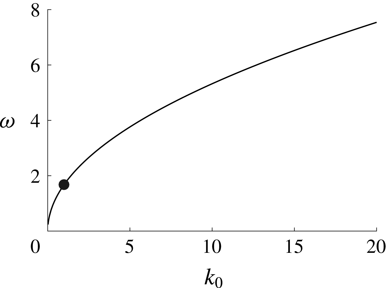
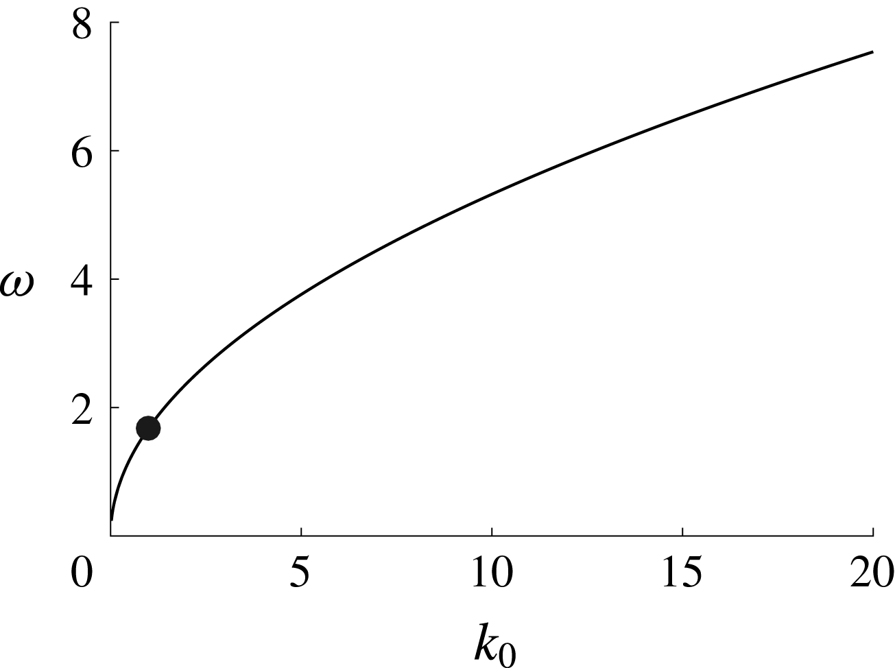
, which corresponds to the presence of an Eulerian counter-flow which counters the effect of the SDV. We plot this zero level set for
 $0\leqslant k_{0}\leqslant 20$
in figure 2. As can be seen, shear strengths which contribute to the suppression of particle drift are always counter-propagating relative to a positively elevated surface.
Plot of the zero set
 $u_{p}^{L}(k_{0},\unicode[STIX]{x1D714})=0$
. The dot denotes the point
 $(k_{0},\unicode[STIX]{x1D714})=(1,1.6818)$
.
At this point, in order to properly couple our mean-surface formulation to the bulk GLM formulation described above, we then require
 $$\begin{eqnarray}\bar{\boldsymbol{u}}^{L}|_{\tilde{z}=\unicode[STIX]{x1D716}\bar{\unicode[STIX]{x1D702}}^{L}}=\bar{\boldsymbol{u}}_{s}^{L}(\tilde{x},t).\end{eqnarray}$$
Thus, we then find the integration constant
 $\tilde{C}(\unicode[STIX]{x1D709},\unicode[STIX]{x1D70F})$
in the formula for the horizontal LDV
 $\bar{u}_{2}^{L}$
to be
 $$\begin{eqnarray}\tilde{C}(\unicode[STIX]{x1D709},\unicode[STIX]{x1D70F})=2k_{0}\unicode[STIX]{x1D714}\left(-s+\frac{\unicode[STIX]{x1D714}}{\unicode[STIX]{x1D6FA}}\right)|\unicode[STIX]{x1D702}_{1}(\unicode[STIX]{x1D709},\unicode[STIX]{x1D70F})|^{2}+\unicode[STIX]{x1D714}\unicode[STIX]{x1D702}_{0}(\unicode[STIX]{x1D709},\unicode[STIX]{x1D70F}).\end{eqnarray}$$
Thus, we can find
 $\bar{u}_{2}^{L}$
as
 $$\begin{eqnarray}\displaystyle \bar{u}_{2}^{L}(\unicode[STIX]{x1D709},\unicode[STIX]{x1D70F},z) & = & \displaystyle 2k_{0}\unicode[STIX]{x1D714}\left(-s+\frac{\unicode[STIX]{x1D714}}{\unicode[STIX]{x1D6FA}}\right)|\unicode[STIX]{x1D702}_{1}(\unicode[STIX]{x1D709},\unicode[STIX]{x1D70F})|^{2}+\unicode[STIX]{x1D714}\unicode[STIX]{x1D702}_{0}(\unicode[STIX]{x1D709},\unicode[STIX]{x1D70F})\nonumber\\ \displaystyle & & \displaystyle \times \,\frac{2\unicode[STIX]{x1D6FA}^{2}}{c_{p}-\unicode[STIX]{x1D714}z}\left(2+\frac{3\unicode[STIX]{x1D714}}{|k_{0}|(c_{p}-\unicode[STIX]{x1D714}z)}+\frac{2\unicode[STIX]{x1D714}^{2}}{k_{0}^{2}(c_{p}-\unicode[STIX]{x1D714}z)^{2}}\right)|\unicode[STIX]{x1D702}_{1}(\unicode[STIX]{x1D709},\unicode[STIX]{x1D70F})|^{2}\text{e}^{2|k_{0}|z}.\nonumber\\ \displaystyle & & \displaystyle\end{eqnarray}$$
We note that if we take the vorticity
 $\unicode[STIX]{x1D714}=0$
, we then get for a left-travelling wave
 $$\begin{eqnarray}\bar{u}_{2}^{L}(\unicode[STIX]{x1D709},\unicode[STIX]{x1D70F},z)=-4k_{0}\unicode[STIX]{x1D6FA}|\unicode[STIX]{x1D702}_{1}(\unicode[STIX]{x1D709},\unicode[STIX]{x1D70F})|^{2}\text{e}^{2|k_{0}|z}.\end{eqnarray}$$
Thus, at zero vorticity, we recreate the classic result for the Stokes drift in an irrotational fluid; see Longuet-Higgins (Reference Longuet-Higgins1953). Likewise, even in the case of zero vorticity, we see the impact of the slowly varying envelope introduced by the NLS equation in the need to solve the, in part, slow-variable-dependent FMEs, which allows for a more complex relationship between
 $\bar{\boldsymbol{u}}_{2}^{L}$
and the pseudomomentum; see Bühler (Reference Bühler2009) for further discussion of this issue. We likewise note that it is in Bühler (Reference Bühler2009) that one sees a clear program for determining
 $\bar{\boldsymbol{u}}^{L}$
via the vorticity and divergence equations we used above in the FMEs. The contribution presented herein was in clearly connecting the FMEs to the lifted surface equations, thereby allowing for the connection of the bulk mean velocity to an unambiguously averaged surface result and a continuously defined LDV.
Following Andrews & McIntyre (Reference Andrews and McIntyre1978), we define the Stokes drift of a quantity, say
 $\bar{\unicode[STIX]{x1D711}}^{S}$
to be
 $$\begin{eqnarray}\bar{\unicode[STIX]{x1D711}}^{S}=\bar{\unicode[STIX]{x1D711}}^{L}-\bar{\unicode[STIX]{x1D711}}.\end{eqnarray}$$
Thus, if we average the fluid velocity in the bulk of the fluid, equations (2.60) and (2.61) show that the bulk Eulerian-mean horizontal velocity is given by
 $\bar{u}(\unicode[STIX]{x1D709},\unicode[STIX]{x1D70F},z)$
where
 $$\begin{eqnarray}\bar{u}(\unicode[STIX]{x1D709},\unicode[STIX]{x1D70F},z)=\unicode[STIX]{x1D714}z+O(\unicode[STIX]{x1D716}^{3}).\end{eqnarray}$$
Thus, in the bulk, the horizontal SVD, say
 $\bar{u}_{2}^{S}(\unicode[STIX]{x1D709},\unicode[STIX]{x1D70F},z)=\bar{u}_{2}^{L}(\unicode[STIX]{x1D709},\unicode[STIX]{x1D70F},z)$
. We emphasize that
 $z$
is a mean coordinate, and thus we do not evaluate the LVD or SVD at the free surface
 $z=\unicode[STIX]{x1D716}\unicode[STIX]{x1D702}(x,t)$
, but instead at the lifted surface
 $\tilde{z}=\unicode[STIX]{x1D716}\bar{\unicode[STIX]{x1D702}}^{L}$
. Near the lifted free surface, by removing the Eulerian-mean term
 $\unicode[STIX]{x1D714}\unicode[STIX]{x1D702}_{0}$
, we have that the surface SDV in the horizontal direction, say
 $\bar{u}_{s}^{S}$
is
 $$\begin{eqnarray}\bar{u}_{s}^{S}(\unicode[STIX]{x1D709},\unicode[STIX]{x1D70F})=-2\unicode[STIX]{x1D716}^{2}k_{0}\unicode[STIX]{x1D6FA}\left(1+\left(1-\frac{s\unicode[STIX]{x1D714}}{\unicode[STIX]{x1D6FA}}\right)^{2}\right)|\unicode[STIX]{x1D702}_{1}(\unicode[STIX]{x1D709},\unicode[STIX]{x1D70F})|^{2}.\end{eqnarray}$$
Note, this multi-part definition for the SDV reflects the intricacies of averaging around a freely evolving surface. This explains our privileging of the LDV over the SDV. Our result then provides support for the phenomenological choices of how the SDV of a plane-wave varies in depth made in Breivik et al. (Reference Breivik, Janssen and Bidlot2014). There, the classic formula for the SDV was modified by multiplying it by terms like
 $1/(1+\tilde{c}z)$
, where
 $\tilde{c}$
was then chosen to improve agreements with observed data. Our result provides a physical motivation for the appearance of such terms. However, while we can put forth a physical mechanism, whether unresolved shear currents near the surface are truly responsible for disagreements between theory and observation is a matter for future work.
3.4 The surface SDV for modulated surface waves
The surface SDV in (3.46) for the Jacobi elliptic function solutions with
 $\unicode[STIX]{x1D6FD}=1$
is given by
 $$\begin{eqnarray}\bar{u}_{s}^{S}(\unicode[STIX]{x1D709},\unicode[STIX]{x1D70F})=-4\unicode[STIX]{x1D716}^{2}\unicode[STIX]{x1D705}^{2}k_{0}\unicode[STIX]{x1D6FA}\left|\frac{\unicode[STIX]{x1D6FC}_{d}}{\unicode[STIX]{x1D6FC}_{nl}}\right|\left(1+\left(1-\frac{s\unicode[STIX]{x1D714}}{\unicode[STIX]{x1D6FA}}\right)^{2}\right)\unicode[STIX]{x1D719}(\unicode[STIX]{x1D709};\unicode[STIX]{x1D705}),\end{eqnarray}$$
where
 $$\begin{eqnarray}\unicode[STIX]{x1D719}(\unicode[STIX]{x1D709};\unicode[STIX]{x1D705})=\left\{\begin{array}{@{}l@{}}\text{cn}^{2}(\unicode[STIX]{x1D709};\unicode[STIX]{x1D705}),\quad \unicode[STIX]{x1D6FC}_{d}/\unicode[STIX]{x1D6FC}_{nl}>0,\\ \text{sn}^{2}(\unicode[STIX]{x1D709};\unicode[STIX]{x1D705}),\quad \unicode[STIX]{x1D6FC}_{d}/\unicode[STIX]{x1D6FC}_{nl}<0,\end{array}\right.\end{eqnarray}$$
where
 $\unicode[STIX]{x1D709}$
is defined in (2.21). Defining the parameter
 $$\begin{eqnarray}\tilde{u} ^{S}(k_{0},\unicode[STIX]{x1D714})=-4k_{0}\unicode[STIX]{x1D6FA}(k_{0},\unicode[STIX]{x1D714})\left|\frac{\unicode[STIX]{x1D6FC}_{d}(k_{0},\unicode[STIX]{x1D714})}{\unicode[STIX]{x1D6FC}_{nl}(k_{0},\unicode[STIX]{x1D714})}\right|\left(1+\left(1-\frac{s\unicode[STIX]{x1D714}}{\unicode[STIX]{x1D6FA}(k_{0},\unicode[STIX]{x1D714})}\right)^{2}\right),\end{eqnarray}$$
and choosing the positive branch of the dispersion relationship, figure 3 shows that this term exhibits a wide variation in magnitude. The curves along which the largest magnitudes are seen correspond to the level set
 $\unicode[STIX]{x1D6FC}_{nl}(k_{0},\unicode[STIX]{x1D714})=0$
. Thus, for the class of Jacobi elliptic solutions, there appears to be a kind of nonlinear resonance between the shear current and the carrier wave. We point out that along this curve, however, the assumptions we used to derive the NLS equation are no longer valid. Therefore, more work should be done to better elucidate the affiliated dynamics associated with parameter choices defining said curve. Throughout the remainder of this paper, we choose parameter values that do not place us too close to the zero set of
 $\unicode[STIX]{x1D6FC}_{nl}(k_{0},\unicode[STIX]{x1D714})=0$
.
Log plot of the surface SDV parameter
 $\tilde{u} ^{S}(k_{0},\unicode[STIX]{x1D714})$
. The curves along which
 $\tilde{u} ^{S}(k_{0},\unicode[STIX]{x1D714})=0$
mirror the transitions between MI stable and unstable regions seen in figure 1. The surface SDV is most augmented near the curves corresponding to
 $\unicode[STIX]{x1D6FC}_{nl}(k_{0},\unicode[STIX]{x1D714})=0$
.
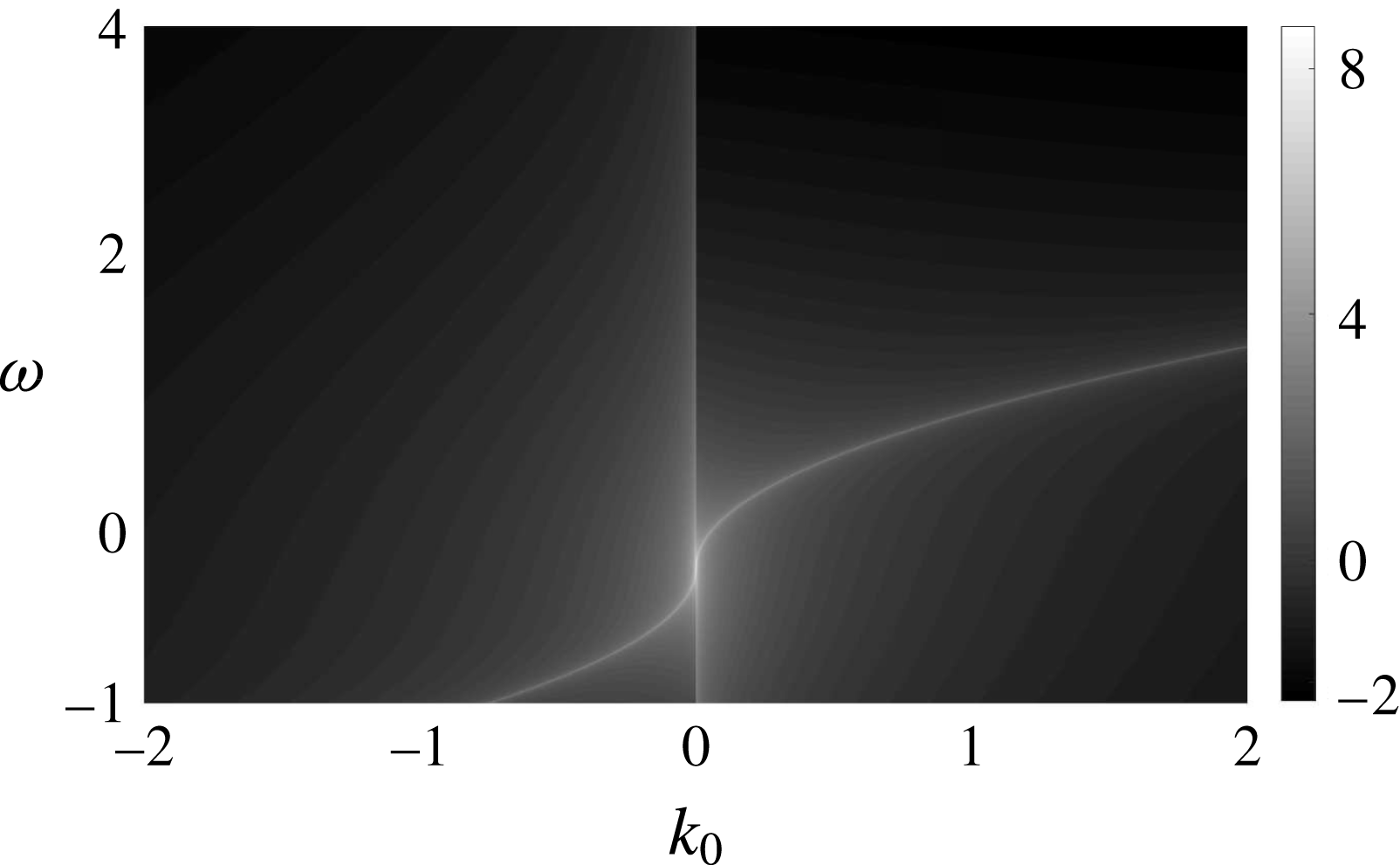
To get a more detailed understanding of how the surface SDV depends on the shear current strength, we choose
 $k_{0}=1$
and use the positive branch of the dispersion relationship. Figure 4 contains plots of
 $\tilde{u} ^{S}(1,\unicode[STIX]{x1D714})$
for
 $-1\leqslant \unicode[STIX]{x1D714}\leqslant 4$
,
 $-1\leqslant \unicode[STIX]{x1D714}\leqslant 1.1$
, and
 $1.2\leqslant \unicode[STIX]{x1D714}\leqslant 4$
. We choose these particular ranges of shear values to in particular examine the behaviour of
 $\tilde{u} ^{S}$
around the resonance curve seen in figure 3. The singularity seen in figure 4(a) corresponds to the value
 $\unicode[STIX]{x1D714}$
such that
 $\unicode[STIX]{x1D6FC}_{nl}(1;\unicode[STIX]{x1D714})=0$
, namely
 $\unicode[STIX]{x1D714}\approx 1.1550$
. Figure 4(b) shows the focusing side and that increasing the shear strength increases the Stokes drift velocity. Figure 4(c) shows that this relationship is reversed on the defocusing side.
Plots of
 $\tilde{u} ^{S}(1,\unicode[STIX]{x1D714})$
for
 $-1\leqslant \unicode[STIX]{x1D714}\leqslant 4$
(a),
 $-1\leqslant \unicode[STIX]{x1D714}\leqslant 1.12$
(b) and
 $1.17\leqslant \unicode[STIX]{x1D714}\leqslant 4$
(c). Note,
 $\unicode[STIX]{x1D6FC}_{nl}(1;1.1550)=0$
. This shows that the magnitude of the SDV increases with increasing shear on the focusing side of the singularity (b), and decreases with increasing shear on the defocusing side (c).
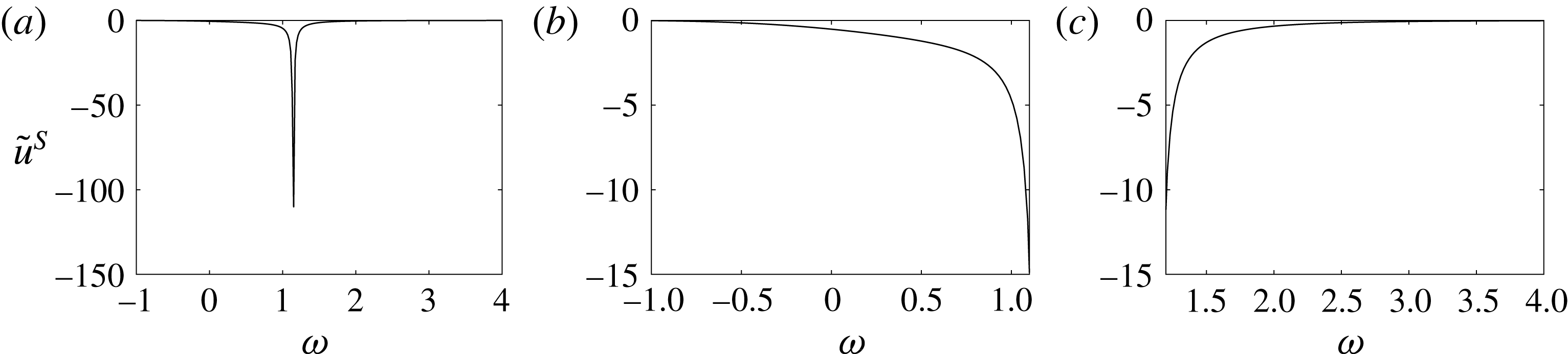
3.5 Flow near the depth
$z_{c}$

Again the depth
 $z_{c}=c_{p}/\unicode[STIX]{x1D714}$
is the depth at which our approximations to the mean particle path fluctuations in (3.19) and (3.20) are no longer valid. Taking
 $k_{0}\unicode[STIX]{x1D714}>0$
so that
 $-\infty <z_{c}<-1$
, it is illuminating to attempt to examine particle paths near this depth. To do this, we look at the special case of a plane-wave solution to the NLS equation, so that we can readily write
 $$\begin{eqnarray}\left.\begin{array}{@{}c@{}}{\dot{x}}=\unicode[STIX]{x1D714}z-2\unicode[STIX]{x1D716}s\unicode[STIX]{x1D6FA}A\text{e}^{|k_{0}|z}\cos (\tilde{\unicode[STIX]{x1D703}})+O(\unicode[STIX]{x1D716}^{2})\\ {\dot{z}}=-2\unicode[STIX]{x1D716}\unicode[STIX]{x1D6FA}A\text{e}^{|k_{0}|z}\sin (\tilde{\unicode[STIX]{x1D703}})+O(\unicode[STIX]{x1D716}^{2}),\end{array}\right\}\end{eqnarray}$$
where
 $\tilde{\unicode[STIX]{x1D703}}=\unicode[STIX]{x1D703}+\unicode[STIX]{x1D716}^{2}\unicode[STIX]{x1D6FC}_{nl}A^{2}t$
. At this order, we can rewrite this system as
 $$\begin{eqnarray}\left.\begin{array}{@{}c@{}}\dot{\tilde{\unicode[STIX]{x1D703}}}=\unicode[STIX]{x1D6FA}+k_{0}\unicode[STIX]{x1D714}z-2\unicode[STIX]{x1D716}|k_{0}|\unicode[STIX]{x1D6FA}A\text{e}^{|k_{0}|z}\cos (\tilde{\unicode[STIX]{x1D703}})+O(\unicode[STIX]{x1D716}^{2}),\\ {\dot{z}}=-2\unicode[STIX]{x1D716}\unicode[STIX]{x1D6FA}A\text{e}^{|k_{0}|z}\sin (\tilde{\unicode[STIX]{x1D703}})+O(\unicode[STIX]{x1D716}^{2}),\end{array}\right\}\end{eqnarray}$$
which to leading order is seen to have the Hamiltonian
 $H(\tilde{\unicode[STIX]{x1D703}},z)$
where
 $$\begin{eqnarray}H(\tilde{\unicode[STIX]{x1D703}},z)=\unicode[STIX]{x1D6FA}z+\frac{k_{0}\unicode[STIX]{x1D714}z^{2}}{2}-2\unicode[STIX]{x1D716}\unicode[STIX]{x1D6FA}A\text{e}^{|k_{0}|z}\cos (\tilde{\unicode[STIX]{x1D703}}).\end{eqnarray}$$
This has critical points at
 $$\begin{eqnarray}\tilde{\unicode[STIX]{x1D703}}=n\unicode[STIX]{x03C0},\quad z=z_{c}-\unicode[STIX]{x1D716}\frac{2c_{p}\text{e}^{|k_{0}|z_{c}}}{\unicode[STIX]{x1D714}}(-1)^{n}+O(\unicode[STIX]{x1D716}^{2}),\end{eqnarray}$$
with even
 $n$
corresponding to centres and odd
 $n$
to saddles. This result then is a good indication for the presence of ‘cats-eye’ patterns around the depth
 $z_{c}$
, a result echoing the works of Simmen & Saffman (Reference Simmen and Saffman1985), Teles da Silva & Peregrine (Reference Teles da Silva and Peregrine1988), Wahlén (Reference Wahlén2009) and Ribeiro et al. (Reference Ribeiro, Milewski and Nachbin2017) among many other authors. This presents an interesting matching problem with regards to finding uniform approximations to the LDV. This however is a question beyond the scope of the present paper.
4 Numerical results
In order to determine particle paths, say
 $(x(t),z(t))$
, in general, the system in (2.48) must be solved. However, we focus on determining particle paths at the surface. Thus, letting
 $\tilde{\unicode[STIX]{x1D702}}$
denote the truncation of (2.20) up to and including
 $O(\unicode[STIX]{x1D716})$
terms, we approximate the vertical component of the path via the restriction
 $$\begin{eqnarray}z(t)=\unicode[STIX]{x1D716}\tilde{\unicode[STIX]{x1D702}}(x(t),t).\end{eqnarray}$$
We then can readily find the scalar equation for the horizontal coordinate
 $x(t)$
to be
 $$\begin{eqnarray}{\dot{x}}=\unicode[STIX]{x1D716}\unicode[STIX]{x1D714}\tilde{\unicode[STIX]{x1D702}}(x,t)+\unicode[STIX]{x1D716}\tilde{\unicode[STIX]{x1D719}}_{x}(x,\unicode[STIX]{x1D716}\tilde{\unicode[STIX]{x1D702}}(x,t),t),\end{eqnarray}$$
where the potential
 $\tilde{\unicode[STIX]{x1D719}}_{x}$
is found using (2.60). However, since the NLS solutions are in terms of the coordinates
 $\unicode[STIX]{x1D709}$
and
 $\unicode[STIX]{x1D70F}$
, we rewrite the above equation in these coordinates so that we have
 $$\begin{eqnarray}\left.\begin{array}{@{}c@{}}{\displaystyle \frac{\text{d}\unicode[STIX]{x1D709}}{\text{d}\unicode[STIX]{x1D70F}}}={\displaystyle \frac{c_{g}}{\unicode[STIX]{x1D716}}}+\unicode[STIX]{x1D714}\tilde{\unicode[STIX]{x1D702}}(\unicode[STIX]{x1D709},\unicode[STIX]{x1D70F})+\tilde{\unicode[STIX]{x1D719}}_{x}(\unicode[STIX]{x1D709},\unicode[STIX]{x1D716}\tilde{\unicode[STIX]{x1D702}}),\\ \unicode[STIX]{x1D709}(0)=\unicode[STIX]{x1D709}_{0}.\end{array}\right\}\end{eqnarray}$$
We use a fourth-order Runge–Kutta (RK4) scheme with a time step of
 $\unicode[STIX]{x1D6FF}\unicode[STIX]{x1D70F}=5\times 10^{-4}$
to solve this initial-value problem. To solve for the evolution of
 $\unicode[STIX]{x1D702}_{1}(\unicode[STIX]{x1D709},\unicode[STIX]{x1D70F})$
, we use a pseudo-spectral scheme with 1024 modes to discretize the VD equation in space thereby allowing it to be coupled to the RK4 scheme used in (4.3). We can then determine
 $\unicode[STIX]{x1D702}_{1}(\unicode[STIX]{x1D709},\unicode[STIX]{x1D70F})$
up to and including
 $O(\unicode[STIX]{x1D716})$
effects on a
 $O(1/\unicode[STIX]{x1D716}^{2})$
time scale. We use the Jacobi elliptic or plane-wave solutions to the NLS equation as an initial condition to the VD equation. By using the VD equation, we see that on the
 $O(1)$
in
 $\unicode[STIX]{x1D70F}$
, or
 $O(1/\unicode[STIX]{x1D716}^{2})$
in
 $t$
, time scale of the NLS equation, we anticipate that the error from truncation in (4.3) should be at worst
 $O(\unicode[STIX]{x1D716}^{2})$
in
 $\unicode[STIX]{x1D709}$
and thus at worst
 $O(\unicode[STIX]{x1D716})$
in
 $x(t)$
. Per our restriction on
 $z(t)$
, this implies that at worst we should anticipate errors of
 $O(\unicode[STIX]{x1D716}^{2})$
on the longer time scales corresponding to the nonlinear effects.
For the Jacobi elliptic function solutions, we chose the initial tracer position to be
 $$\begin{eqnarray}\unicode[STIX]{x1D709}(0)=\frac{K(\unicode[STIX]{x1D705})}{128},\quad z(0)=\unicode[STIX]{x1D716}\tilde{\unicode[STIX]{x1D702}}(\unicode[STIX]{x1D709}(0),0),\end{eqnarray}$$
where
 $K(\unicode[STIX]{x1D705})$
is the complete elliptic integral of the first kind and
 $\tilde{\unicode[STIX]{x1D702}}$
is defined by (2.20). For the plane-wave solutions, we chose
 $\unicode[STIX]{x1D709}_{0}=10/128$
so the initial positions are comparable across the different classes of solutions. We take the positive branch of the dispersion relationship, which implies that
 $k_{0}>0$
corresponds to a left-moving carrier wave. We choose
 $k_{0}=1$
for the plane-wave solutions. In the case of the Jacobi elliptic solutions to the NLS equation, we choose the integer
 $m$
to be
 $$\begin{eqnarray}m=\left\lfloor \frac{2K(\unicode[STIX]{x1D705})}{\unicode[STIX]{x03C0}\unicode[STIX]{x1D716}}\right\rfloor ,\end{eqnarray}$$
so that, using (2.42),
 $k_{0}\approx 1$
. In practice,
 $k_{0}\approx 0.98$
or
 $0.99$
. The results for the tracer position in physical coordinates,
 $(x(t),z(t))$
, are found using the transformations
 $$\begin{eqnarray}x(t)=\frac{\unicode[STIX]{x1D709}(\unicode[STIX]{x1D70F})}{\unicode[STIX]{x1D716}}-\frac{c_{g}\unicode[STIX]{x1D70F}}{\unicode[STIX]{x1D716}^{2}},\quad t=\frac{\unicode[STIX]{x1D70F}}{\unicode[STIX]{x1D716}^{2}}.\end{eqnarray}$$
Fourier transforms and their inverses are computed numerically using the fast Fourier transform.
Finally, the expansions in (2.60) and (2.61), and the associated approximations in (2.62) and (2.63), show that the strength of the velocity field is largely determined by the magnitude of the solution to the NLS equation which is the leading-order approximation to
 $\unicode[STIX]{x1D702}_{1}$
. In the case of the Jacobi elliptic function solutions, controlling for the elliptic modulus
 $\unicode[STIX]{x1D705}$
, the term
 $\sqrt{2|\unicode[STIX]{x1D6FC}_{d}/\unicode[STIX]{x1D6FC}_{nl}|}$
is the most significant contribution to the magnitude of
 $\unicode[STIX]{x1D702}_{1}$
since we have fixed
 $\unicode[STIX]{x1D6FD}=1$
; see (2.38) and (2.40). Figure 5 contains plots of
 $\sqrt{2|\unicode[STIX]{x1D6FC}_{d}/\unicode[STIX]{x1D6FC}_{nl}|}$
versus
 $\unicode[STIX]{x1D714}$
for
 $k_{0}=1$
. Note, we take
 $\unicode[STIX]{x1D714}=O(1)$
to be consistent with our derivation of the VD equation. In the focusing case, increasing the magnitude of the Jacobi elliptic function solutions corresponds to increasing the shear strength. In the defocusing case, decreasing the magnitude of the Jacobi elliptic function solutions corresponds to increasing the shear strength. These two statements are justified by the similarities of figures 5(b,c) and 4(b,c). Therefore, relatively large-amplitude solutions inducing strong fluid particle drift are to be expected near the resonance curve.
Strength of the surface velocity as measured via plots of
 $\sqrt{2|\unicode[STIX]{x1D6FC}_{d}/\unicode[STIX]{x1D6FC}_{nl}|}$
for
 $k_{0}=1$
for
 $-1\leqslant \unicode[STIX]{x1D714}\leqslant 4$
(a),
 $-1\leqslant \unicode[STIX]{x1D714}\leqslant 1.12$
(b) and
 $1.17\leqslant \unicode[STIX]{x1D714}\leqslant 4$
(c). Increasing shear increases the velocity on the focusing side, and decreases it on the defocusing side.
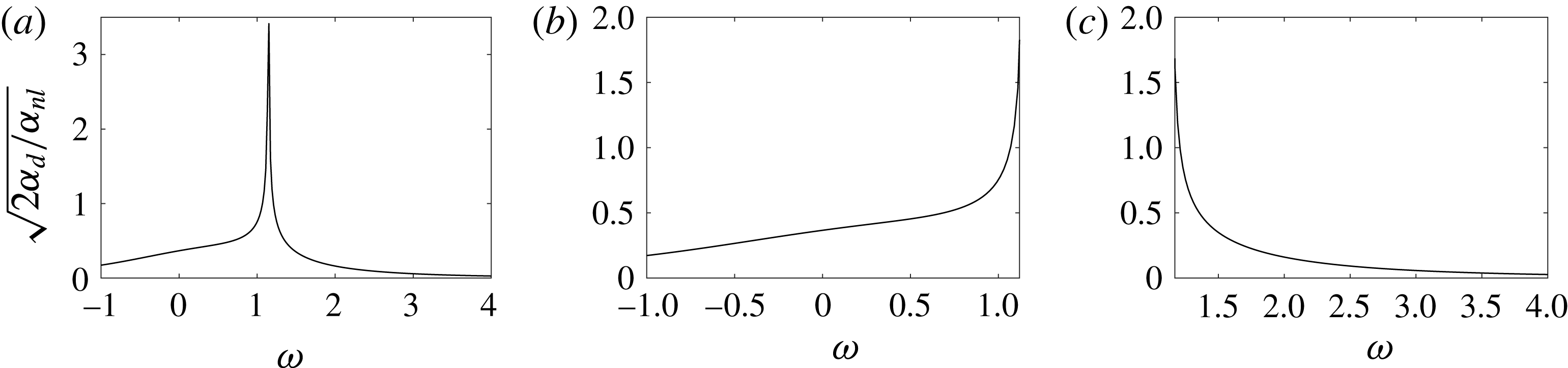
Focusing case – plots of particle paths correspond to the solution given in (2.38) with
 $\unicode[STIX]{x1D716}=0.1$
,
 $\unicode[STIX]{x1D6FD}=1$
,
 $k_{0}\approx 1$
,
 $\unicode[STIX]{x1D705}=0.5$
, with
 $\unicode[STIX]{x1D714}=0$
(a),
 $\unicode[STIX]{x1D714}=1.12$
(b) and
 $\unicode[STIX]{x1D714}=-1$
(c). The grey dots indicate the starting positions of the tracers while the black dots indicate their final positions.
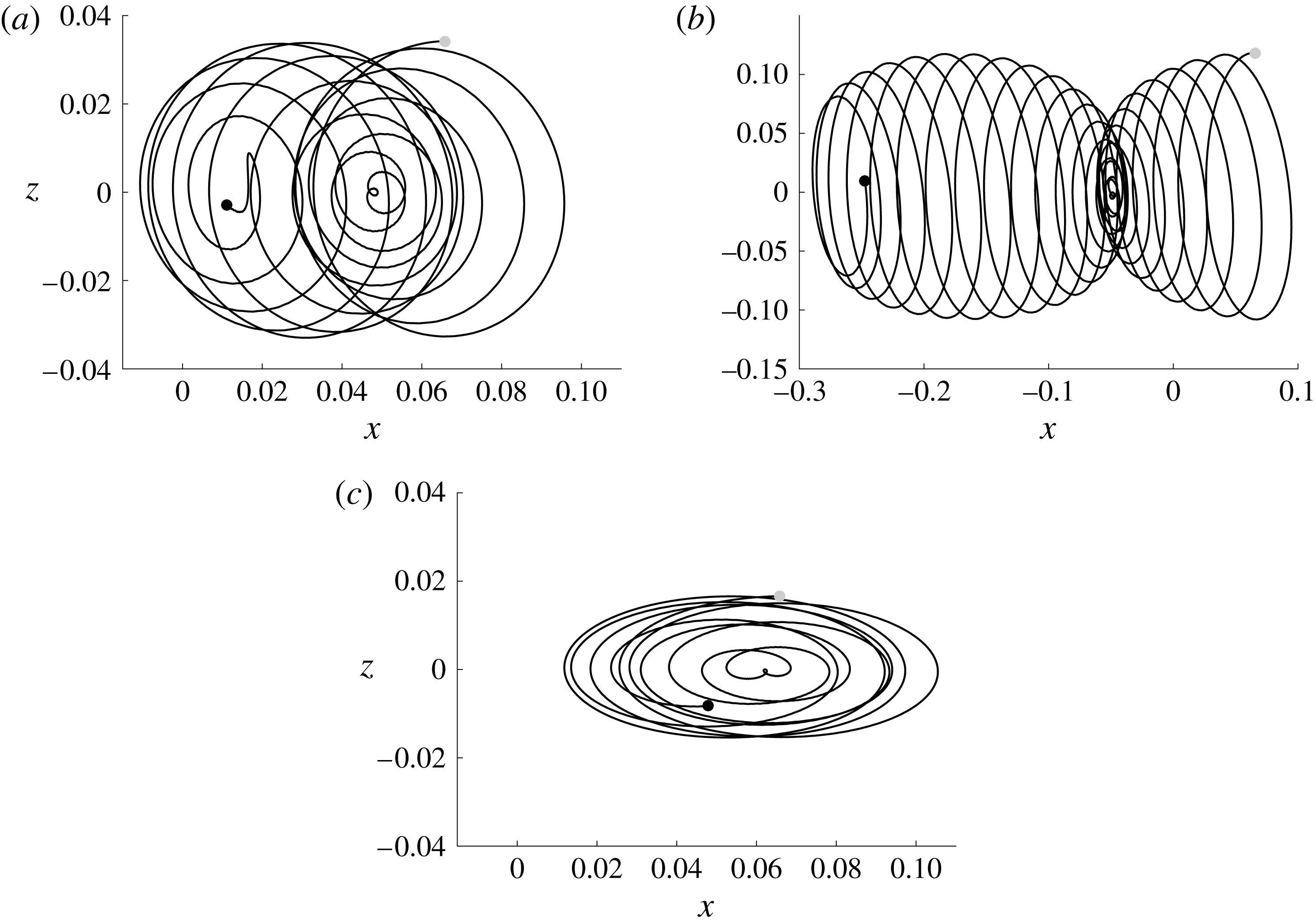
4.1 Focusing case
Using the solution given in (2.38) with
 $k_{0}\approx 1$
ensures that
 $\unicode[STIX]{x1D714}=0$
and
 $\unicode[STIX]{x1D714}=\pm 1$
are in the focusing regime. Figure 6 shows the paths of particles as well as there mean paths for three values of
 $\unicode[STIX]{x1D714}$
found by setting
 $\unicode[STIX]{x1D716}=0.1$
,
 $\unicode[STIX]{x1D705}=0.5$
, and solving the dynamical system for the particle and mean paths up to time
 $t=1/\unicode[STIX]{x1D716}^{2}$
. The carrier profile is propagating to the left in this situation. Therefore, if
 $\unicode[STIX]{x1D714}=1.12$
, then the shear current is counter-propagating at the surface with respect to the carrier wave while if
 $\unicode[STIX]{x1D714}=-1$
, the current is co-propagating. The counter-propagating current significantly enhances the leftward horizontal motion of a tracer along the surface as seen by comparing figures 6(b) and (c) with (a). This can be explained by comparing the values of the SDV and the LDV parameters
 $$\begin{eqnarray}\left.\begin{array}{@{}c@{}}\tilde{u} ^{S}(1,0)=-0.5222,\quad \tilde{u} ^{L}(1,0)=-0.5222,\\ \tilde{u} ^{S}(1,1.12)=-10.7373,\quad \tilde{u} ^{L}(1,1.12)=-5.2195,\\ \tilde{u} ^{S}(1,-1)=-0.2836,\quad \tilde{u} ^{L}(1,-1)=-0.1636,\end{array}\right\}\end{eqnarray}$$
where the parameter
 $\tilde{u} ^{L}$
is defined to be
 $$\begin{eqnarray}\tilde{u} ^{L}(k_{0},\unicode[STIX]{x1D714})=2\left|\frac{\unicode[STIX]{x1D6FC}_{d}(k_{0},\unicode[STIX]{x1D714})}{\unicode[STIX]{x1D6FC}_{nl}(k_{0},\unicode[STIX]{x1D714})}\right|u_{p}^{L}(k_{0},\unicode[STIX]{x1D714}).\end{eqnarray}$$
Note that for the Jacobi elliptic solutions and controlling for
 $\unicode[STIX]{x1D705}$
and
 $\unicode[STIX]{x1D6FD}$
, this will be the most significant contribution to the magnitude of the LDV. This demonstrates why the counter-propagating current so enhances the leftward drift since the LDV parameter is an order of magnitude larger than in the other cases. Further, it demonstrates why the co-propagating current, i.e.
 $\unicode[STIX]{x1D714}=-1$
, reduces the horizontal displacement of the surface particle. This is somewhat surprising as one might intuitively imagine that the co-propagating shear would enhance the particle drift, especially in comparison to the zero-vorticity case. However, we have effectively shown that nonlinearity makes the surface/current interaction a more complicated one than one might at first suspect.
Choosing
 $\unicode[STIX]{x1D705}=0.99$
shows that similar results hold closer to the solitary wave solution; see figure 7, although the larger elliptic modulus results in the larger amplitudes and leftward drifts. In particular, near the solitary wave limit, positive, counter-propagating shear can greatly enhance both the impact of nonlinearity and the transport properties of the waves.
Focusing case – plots of particle paths correspond to the solution given in (2.38) with
 $\unicode[STIX]{x1D716}=0.1$
,
 $\unicode[STIX]{x1D6FD}=1$
,
 $k_{0}\approx 1$
,
 $\unicode[STIX]{x1D705}=0.99$
, with
 $\unicode[STIX]{x1D714}=0$
(a),
 $\unicode[STIX]{x1D714}=1.12$
(b) and
 $\unicode[STIX]{x1D714}=-1$
(c). The grey dot indicates the starting position of the tracer while the black dot indicates the final position.
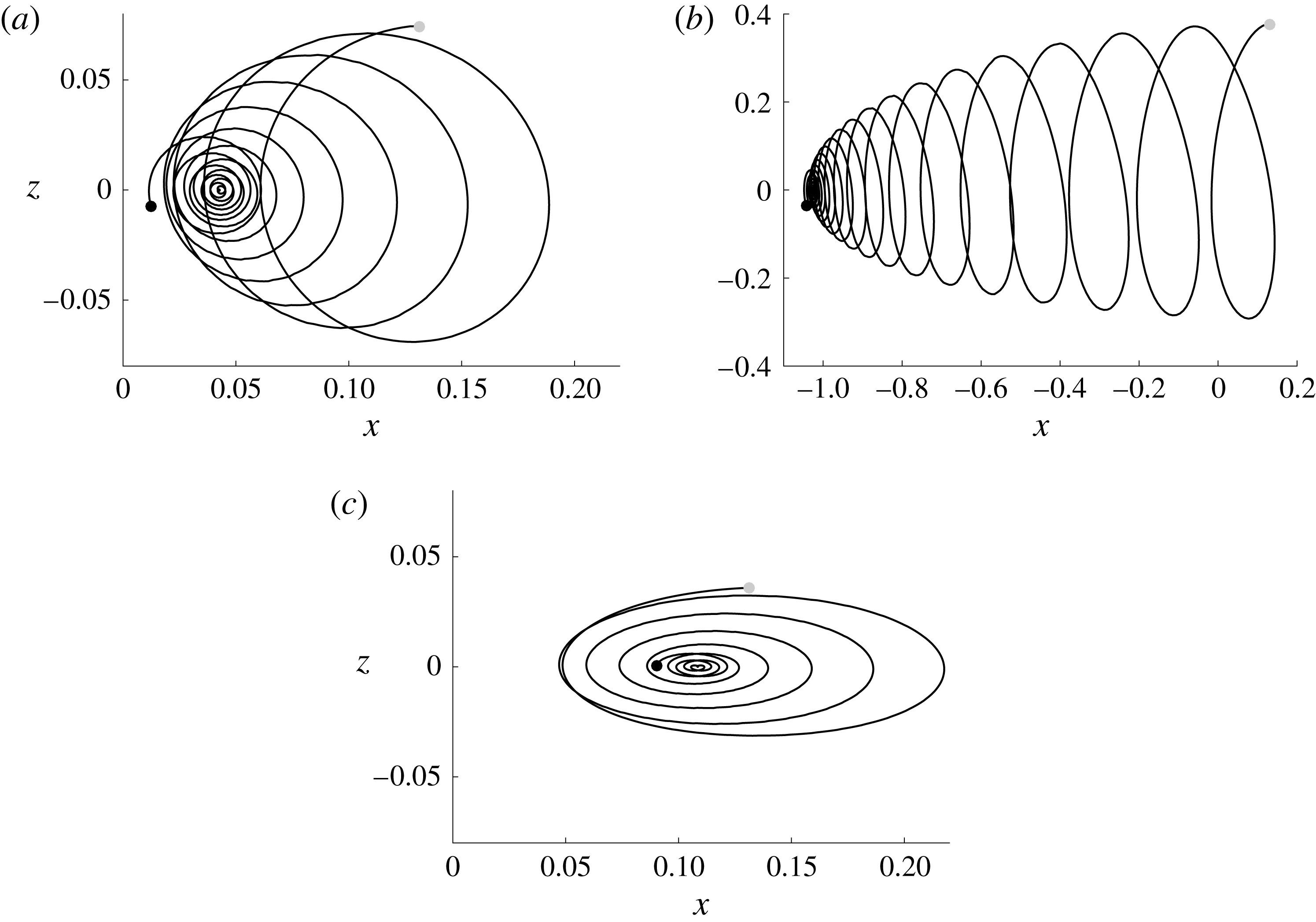
4.2 Defocusing case
For the Jacobi elliptic solutions with
 $k_{0}\approx 1$
, the zero LDV solutions belong in the defocusing case. Figure 8 shows the impact on surface flow particle paths when
 $\unicode[STIX]{x1D714}$
is chosen to zero out the LDV. As can be seen, the particle paths, while not exactly closed, are spirals and are constrained in their horizontal and vertical extent by an outer elliptical perimeter. Similarly, the shear strength can be chosen so that the LDV is zeroed out for the plane-wave solutions. Taking
 $k_{0}=1$
and
 $A=1$
, this corresponds to choosing
 $\unicode[STIX]{x1D714}=1.6828$
. Figure 9 shows a nearly closed particle path. We emphasize that these results are a confirmation of the predictions made in figure 2. Thus, these numerical results validate our choice to generalize the GLM approach in so far as we see the generalization provides the correct predictions for when shear will quench surface drift.
Defocusing case – plots of particle paths correspond to the solution given in (2.40) with
 $\unicode[STIX]{x1D716}=0.1$
,
 $\unicode[STIX]{x1D6FD}=1$
,
 $k_{0}\approx 1$
, with
 $\unicode[STIX]{x1D705}=0.5$
(a),
 $\unicode[STIX]{x1D705}=0.99$
(b). The choices of
 $\unicode[STIX]{x1D714}$
ensure that
 $\tilde{u} ^{L}(1,\unicode[STIX]{x1D714})=0$
, see figure 2, thereby leading to the nearly closed, elliptical particle paths. The grey dots indicate the starting positions of the tracers while the black dots indicate their final positions.
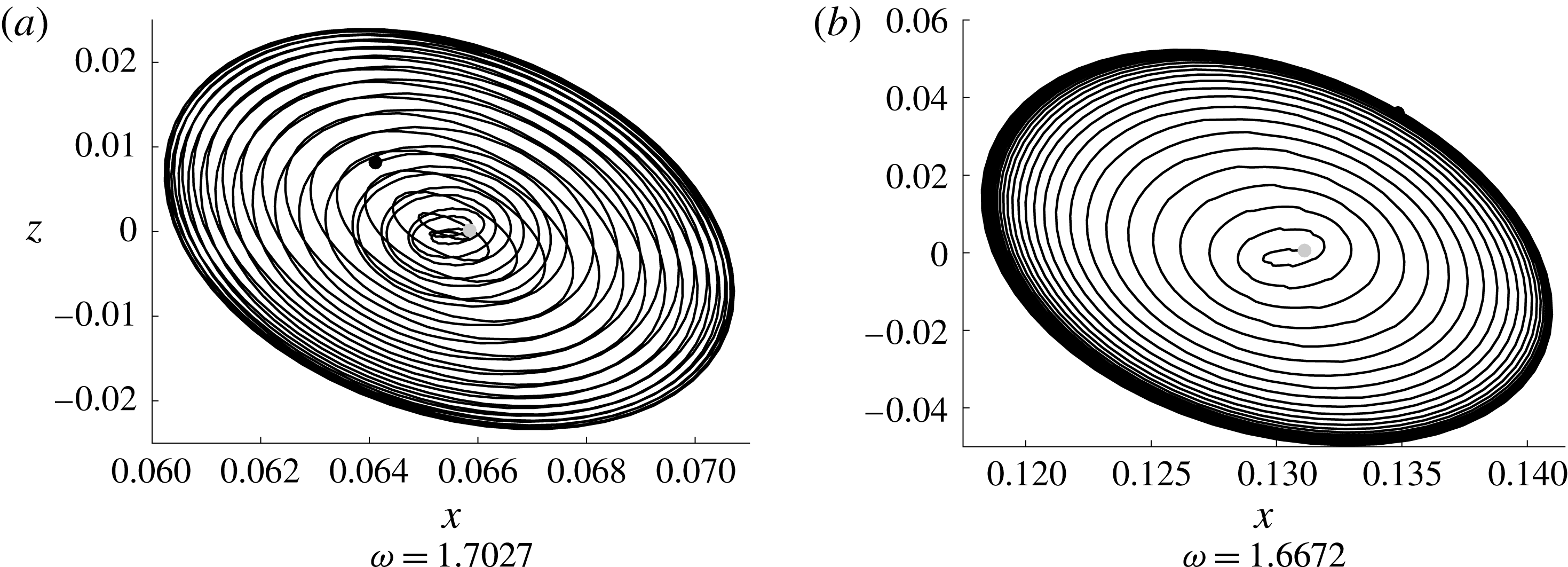
Defocusing case – plot of a particle path corresponding to a plane-wave solution with
 $\unicode[STIX]{x1D716}=0.1$
,
 $A=1$
,
 $k_{0}=1$
and
 $\unicode[STIX]{x1D714}=1.6818$
, which ensures that
 $\tilde{u} ^{L}(1,\unicode[STIX]{x1D714})=0$
, see figure 2, thereby leading to the nearly closed, elliptical particle paths. The grey dots indicate the starting positions of the tracers while the black dots indicate their final positions.
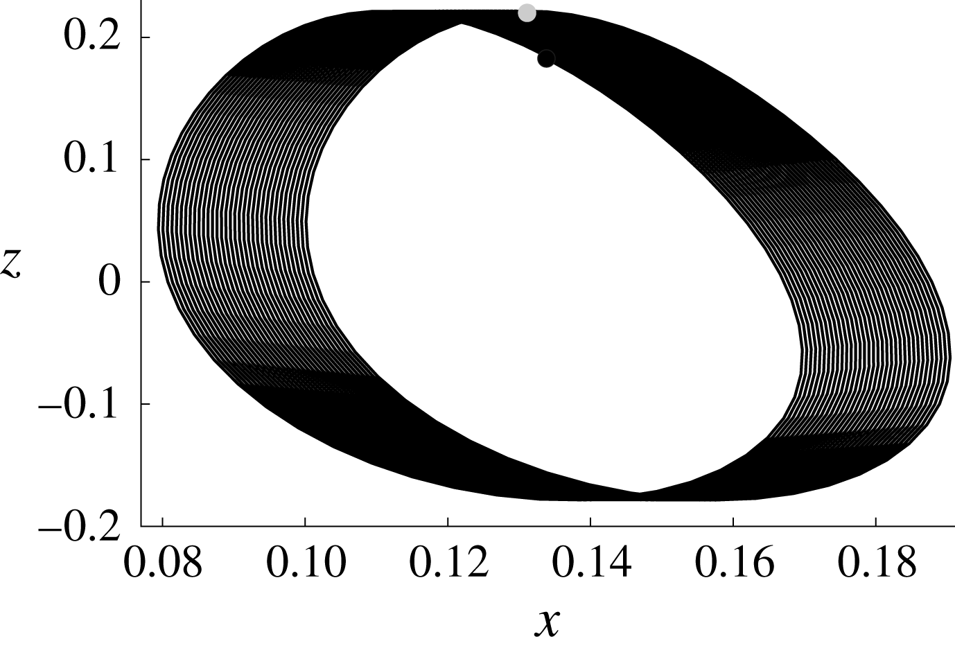
In some respects then, we have also shown that by appropriately choosing the shear, we can replicate the dynamics of a Gerstner wave, see Constantin (Reference Constantin2011) by looking instead at a plane-wave solution moving over a counter-propagating shear current. This could point towards resolving some of the questions raised in Smith (Reference Smith2006) and Monismith et al. (Reference Monismith, Cowen, Nepf, Magnaudet and Thais2007), although this is a subject of future research.
Looking beyond cases in which Eulerian counter-flows quench drift, we now consider the defocusing NLS Jacobi elliptic function solutions given in (2.40). We choose
 $k_{0}\approx 1$
,
 $\unicode[STIX]{x1D716}=0.1$
,
 $\unicode[STIX]{x1D705}=0.99$
(near the dark-soliton limit). Solving the dynamical system for the particle paths up to time
 $t=1/\unicode[STIX]{x1D716}^{2}$
generates figures 10(a) and 10(b) for
 $\unicode[STIX]{x1D714}=1.17$
and
 $\unicode[STIX]{x1D714}=4$
respectively. While the particle path motion seen in figure 10(a) is rapidly oscillating, the net transport and amplitude are quite small.
Defocusing – near dark-soliton solution for
 $k_{0}\approx 1$
,
 $\unicode[STIX]{x1D705}=0.99$
and
 $\unicode[STIX]{x1D714}=1.17$
(a) and
 $\unicode[STIX]{x1D714}=4$
(b). The grey dot indicates the starting position of the tracer while the black dot indicates the final position.

However, if
 $\unicode[STIX]{x1D714}=4$
in the case of a plane wave, we do not necessarily get the same diminished response seen for the Jacobi elliptic solutions; see figure 11. The highly oscillatory plane-wave profile induces a particle path which ultimately exhibits a strong rightward drift which follows the strong counter-propagating shear current. The associated SDV and LDV at the surface for the plane wave with these parameters are given by
 $$\begin{eqnarray}\left.\begin{array}{@{}c@{}}\bar{u}_{s}^{S}=-8.4985\unicode[STIX]{x1D716}^{2}+O(\unicode[STIX]{x1D716}^{3}),\\ \bar{u}_{s}^{L}=29.2719\unicode[STIX]{x1D716}^{2}+O(\unicode[STIX]{x1D716}^{3}).\end{array}\right\}\end{eqnarray}$$
This explains the stronger net rightward drift of the particle shown in figure 11. Finally, note that this shows the SDV and the LDV can oppose one another, thereby clarifying the need to use both velocities to fully understand the drift properties associated with a surface wave.
Defocusing case – plane-wave solution for
 $k_{0}=1$
,
 $\unicode[STIX]{x1D714}=4$
,
 $A=1$
, with (b) providing a detail of (a). The grey dot indicates the starting position of the tracer while the black dot indicates the final position.

5 Conclusion
In this paper, to better understand the transport properties of nonlinear waves moving over constant-vorticity currents, we have derived an asymptotically self-consistent higher-order model for the interaction between the mean wave height and the leading-order modulated carrier wave in the presence of surface tension and a constant-vorticity current. Using this, an NLS equation is derived, and the role of surface tension in determining the existence of modulational instability is fully explored. A formula for the Stokes drift velocity at the surface is derived allowing for the identification of shear profiles which enhance or quench horizontal surface transport. Numerical simulations corroborate the surface theory developed in this paper.
The work in this paper provides possible explanatory mechanisms for otherwise unexplained oceanic phenomena observed in Smith (Reference Smith2006) and justification for phenomenological choices in oceanographic modelling put forward in Breivik et al. (Reference Breivik, Janssen and Bidlot2014). Assessing how accurately a constant-vorticity modulational nonlinear wave model describes these real world problems is an important future research direction. Likewise, while a higher-order model describing the coupled evolution of the mean and modulated carrier wave is derived, the properties of this equation are not studied directly.
Acknowledgements
This material is based upon work supported by the National Science Foundation under grant no. DMS-1439786 while C.W.C. and J.D.C. were in residence at the Institute for Computational and Experimental Research in Mathematics in Providence, RI, during the Spring 2017 semester. Additionally, J.D.C. acknowledges and thanks the Norwegian Fulbright Core Scholar Program for supporting his five month long visit to the University of Bergen to work with H.K. This research was also supported by the Research Council of Norway through grants 213474/F20 and 239033/F20. We also express a great gratitude towards the anonymous reviewers whose comments and questions helped this become a far stronger paper.