







1. Introduction
Gravity currents (GCs) are generated by density differences and appear when a fluid of given density  $\rho$ advances into an ambient fluid of different density
 $\rho \pm \Delta \rho$, and the flow is primarily horizontal (Simpson Reference Simpson1997).
The phenomenon of GCs, ubiquitous in nature and industrial processes, has generated a large body of literature, very difficult to fully review; examples of partial reviews, geared towards specific topics, are Huppert (Reference Huppert1998), Griffiths (Reference Griffiths2000), Moodie (Reference Moodie2002), Huppert (Reference Huppert2006), Chowdhury & Testik (Reference Chowdhury and Testik2014), Riaz & Cinar (Reference Riaz and Cinar2014), Lauriola et al. (Reference Lauriola, Felisa, Petrolo, Di Federico and Longo2018), Ungarish (Reference Ungarish2018) and Lube et al. (Reference Lube, Breard, Esposti-Ongaro, Dufek and Brand2020).
In particular, gravity-driven flows in porous media, well summarized in the book by Woods (Woods Reference Woods2015), attract interest given the wealth of associated energy and environmental applications, such as CO $_2$ sequestration (Huppert & Neufeld Reference Huppert and Neufeld2014), reservoir (oil and gas) engineering (De Loubens & Ramakrishnan Reference De Loubens and Ramakrishnan2011), underground hydrogen storage (Sheikhi, Sahu & Flynn Reference Sheikhi, Sahu and Flynn2023), geothermal power production (Woods Reference Woods1999) and the transport of pollutants such as non-aqueous phase liquids (Schneider et al. Reference Schneider, di Chiara Roupert, Schaefer and Helluy2015) in the subsurface environment generated by the chemical, mining (drilling fluids, see Li et al. Reference Li, Lockington, Parlange, Stagnitti, Jeng, Selker, Telyakovskiy, Barry and Parlange2005) or nuclear industry.
Gravity currents in porous media are viscosity/buoyancy-dominated and typically propagate over (or below) an impermeable bottom (or top) layer, depending whether the intruding current is heavier or lighter than the ambient fluid. Alternatively, the bottom or top limiting layer can be leaky, due to its permeable nature or to one or more draining fracture(s). The ambient fluid is mostly taken to be homogeneous (for the case of ambient stratifications, see Pegler, Huppert & Neufeld (Reference Pegler, Huppert and Neufeld2016)) and often to be immobile, i.e. neglecting return flows (see e.g. Matson & Hogg Reference Matson and Hogg2012); this assumption is typically acceptable in the unconfined schematization, with a current depth much less than the thickness of the host layer. The reference frame is usually non-rotating; the base geometry of the flow can be axisymmetric or plane, the former associated with a line of injecting wells, the latter to a single injection well. For these two base flows, simple similarity solutions by Huppert & Woods (Reference Huppert and Woods1995) and Lyle et al. (Reference Lyle, Huppert, Hallworth, Bickle and Chadwick2005) are available to describe the intermediate-time behaviour of the current. When the geometry becomes more complicated, the influence of boundaries (Zheng & Stone Reference Zheng and Stone2022) or topographic controls (Pegler, Huppert & Neufeld Reference Pegler, Huppert and Neufeld2013) may be incorporated into the conceptual scheme, leading to semianalytical or numerical solutions of the one-dimensional (1-D) transient propagation.
The search for realism in the conceptualization of GCs in porous media has directed researchers also to consider variants to the flow law commonly adopted, i.e. Darcy's law. On one hand, non-Newtonian behaviour of the intruding fluid was considered, and a corresponding extension to Darcy's law adopted, first upon extending the base solution for plane geometry and Newtonian flow first reported in Huppert & Woods (Reference Huppert and Woods1995) to power-law rheological behaviour (Di Federico, Archetti & Longo Reference Di Federico, Archetti and Longo2012), then upon developing solutions for more complex geometries, boundary conditions and types of flow (Longo et al. (Reference Longo, Chiapponi, Petrolo, Lenci and Di Federico2021) and references therein). On the other hand, flow in the vicinity of pumping/injecting wells or in coarse porous media is often best described by a nonlinear equation usually known as Darcy–Forchheimer, where an additional term quadratic in the seepage velocity appears in addition to the linear forcing term incorporating permeability. The term was added empirically by Forchheimer (Reference Forchheimer1901), while theoretical derivations of Darcy, and Darcy–Forchheimer equations from first principles, are reported in Neuman (Reference Neuman1977) and Whitaker (Reference Whitaker1996), respectively.
The Darcy–Forchheimer regime is characteristic, in nature, of conglomerate-confined aquifers, composed of conglomerate, coarse sandstone, as happens in the area of the Ordos Basin (Zhang et al. Reference Zhang, Fan, Ma and Wang2011, Reference Zhang, Zhao, Gan, Yuan, Zhu, Cai and Cao2018). Further, non-Darcy flow represents a significant challenge to the productivity of hydraulically fractured reservoirs, including those containing shale gas, tight oil and geothermal water formations (Barree & Conway Reference Barree and Conway2004). Darcy–Forchheimer flow is also relevant in the screening and selection of sites for  $\textrm {CO}_2$ sequestration (Mathias et al. Reference Mathias, Hardisty, Trudell and Zimmerman2009a), and can be also observed in open-graded asphalt pavements; these provide rapid runoff of rainwater, thereby enhancing safety and visibility (Autelitano et al. Reference Autelitano, Petrolo, Chiapponi, Giuliani and Longo2022). In all these examples, an injected fluid may displace an ambient fluid and advance into the porous medium (also) by virtue of density differences. It seems therefore both of practical and of general interest to extend the study of the propagation of GCs in porous media to the Darcy–Forchheimer regime. Here we focus on a sharp interface schematization of the GC, and derive a semianalytical model considering the influence of Forchheimer effects on the propagation of plane GCs in an infinite domain. To the best of our knowledge, the only works on GCs incorporating Darcy–Forchheimer flow are Mathias et al. (Reference Mathias, Hardisty, Trudell, Zimmerman and Carrera2009b) and the aforementioned study by Mathias et al. (Reference Mathias, Hardisty, Trudell and Zimmerman2009a), simulating
 $\text {CO}_2$ injection and heat transport in a porous domain of infinite cylindrical geometry and finite height, and taking into account the fluid compressibility; the scheme was modified by Mathias et al. (Reference Mathias, de Miguel Gonzalez Martinez, Thatcher and Zimmerman2011) and Mathias, McElwaine & Gluyas (Reference Mathias, McElwaine and Gluyas2014) to account for a finite rather than infinite domain. In all these cases, the flow law is used in a purely numerical context, so none of these studies undermines the novelty of the present manuscript. In fact, three important differences are considered here: (i) the geometry is plane rather than radial, as in the former case the high seepage velocities necessary to invoke the Forchheimer correction are more likely to be reached in the whole flow domain than in the latter case; (ii) the aquifer subject to injection is of infinite height, hence the flow is free-surface throughout the entire flow domain, as in the two earliest seminal studies on porous GC (Huppert & Woods Reference Huppert and Woods1995; Lyle et al. Reference Lyle, Huppert, Hallworth, Bickle and Chadwick2005) – this restricts the solution's applicability but renders more plausible the no-flow assumption within the ambient fluid; (iii) no compressibility effects are considered (partially a consequence of the previous assumption), and the emphasis is on the difference with the classical approach using Darcy's law in the first study on porous GCs in plane geometry (Huppert & Woods Reference Huppert and Woods1995).
The adoption of the Darcy–Forchheimer expression in lieu of Darcy's entails the presence of a second source of nonlinearity in the approach, other than that associated with free-surface flow. The nonlinear flow law is then approximated in two limit cases, corresponding to a local Forchheimer number much lower or larger than unity, respectively; in the former case, the flow law is also linearized. Both cases allow the reduction of the partial differential equation (PDE) governing the 1-D transient flow of the GC to an ordinary differential equation (ODE) and are thus amenable to classical, late-time similarity solutions when coupled with the integral boundary condition describing the increase of the volume of the current as a power of time of exponent  $\gamma$. Results stemming from the solution of these ODEs compare favourably with those deriving from the numerical integration of the original PDEs.
The paper is organized as follows. In § 2, the fundamentals of Darcy–Forchheimer flow are revised, and the GC problem is formulated in plane geometry. In § 3, the problem is solved in semianalytical form with said approximations for  $\gamma \neq 2$, while § 4 presents fully analytical results for
 $\gamma =2$. The approximate solutions are corroborated with full numerical results in § 5. Section 6 describes the experiments conducted to check our theoretical models. We draw conclusions and provide indications for future work in § 7. Appendix A provides details on the structure and typical ranges of the dimensionless parameter summarizing problem parameters and governing the formulation, Appendix B presents an alternative expression for the average slope of the current, while Appendix C illustrates the derivation of the self-similar solution for low local Forchheimer number in a more general context.
2. Materials and methods
2.1. Darcy–Forchheimer flow in porous media
High-velocity filtration flow, termed also inertial in the literature (and having nothing to do with inertial GCs), in isotropic porous media is usually described by the Darcy–Forchheimer equation, reading in vectorial form (Forchheimer Reference Forchheimer1901)
 \begin{equation} \boldsymbol{\nabla} p-\rho \boldsymbol{g}={-}\left(\frac{\mu}{k}+\rho\beta\left|\boldsymbol{u}\right|\right)\boldsymbol{u}={-}\left(\alpha+\rho\beta\left|\boldsymbol{u}\right|\right)\boldsymbol{u}, \end{equation}
where  $p$ is the pressure,
 $\boldsymbol {g}\equiv (0,0,-g)$ is the gravity,
 $\boldsymbol {u}$ is the Darcy velocity of modulus
 $|\boldsymbol {u}|=\sqrt {\boldsymbol {u}\boldsymbol {\cdot }\boldsymbol {u}}$,
 $\rho$ and
 $\mu$ are the fluid density and dynamic viscosity,
 $k\,([k]=[L^2])$ is the medium permeability,
 $\alpha =\mu /k$ and
 $\beta \,([\beta ]=[L^{-1}])$ is the Forchheimer or inertial factor, having an empirical nature. Literature methods for determining
 $\beta$ are either based on direct experimental measurement, or assume a direct correlation between
 $\beta$ and other intrinsic properties of the porous medium, such as porosity and permeability (Lenci, Zeighami & Di Federico Reference Lenci, Zeighami and Di Federico2022). On the basis of dimensional analysis, it can be proven that (Autelitano et al. Reference Autelitano, Petrolo, Chiapponi, Giuliani and Longo2022)
 \begin{equation} \beta=C_D\left(\frac{\rho g }{\mu K}\right)^{1/2}\equiv\frac{C_D}{k^{1/2}}, \end{equation}
being  $K=(\rho g k)/\mu = gk/\nu \,([K]=[LT^{-1}])$ the hydraulic conductivity,
 $\nu =\mu /\rho$ the kinematic viscosity and
 $C_D$ the form-drag dimensionless coefficient. More general forms of (2.1) describe flow in anisotropic media (Whitaker Reference Whitaker1996; Garibotti & Pészynska Reference Garibotti and Pészynska2009); see also Lasseux & Valdés-Parada (Reference Lasseux and Valdés-Parada2017) for a review of historical developments aimed at representing nonlinear effects in porous media flow.
Equation (2.1) can be formulated in terms of hydraulic head  $h=z+p/(\rho g)$ as
 \begin{equation} \boldsymbol{\nabla} h={-}\left(\frac{1}{K}+\frac{\beta}{g}\left|\boldsymbol{u}\right|\right)\boldsymbol{u}. \end{equation}
When  $\beta =0$, (2.1) and (2.3) revert to Darcy's law, governing the purely viscous regime in porous media flow. In practice, the transition between the viscous and the inertial regime is governed by the Forchheimer number
 $Fo=(k\beta \rho |\boldsymbol {u}|)/\mu$, equal to the ratio of liquid–solid interaction to viscous resistance (Ruth & Ma Reference Ruth and Ma1992); values of
 $Fo$ of order 0.11 entail an error of ignoring non-Darcy behaviour of
 $10\,\%$ according to Zheng & Grigg (Reference Zheng and Grigg2006). Note that
 $k$ in (2.2) is the Forchheimer permeability
 $k_F$, which is close, but not the same as, the Darcy permeability
 $k_D$ appearing in the isotropic form of Darcy's law
 $\boldsymbol {\nabla } p-\rho \boldsymbol {g}=-(\mu /k_D)\boldsymbol {u}$ (Muljadi et al. Reference Muljadi, Blunt, Raeini and Bijelic2017; El-Zehairi et al. Reference El-Zehairi, Mousavi-Nehzad, Joekar-Niasar, Guymer, Kourra and Williams2019). Henceforth and in the previous relationships, this difference is neglected on grounds of the smallness of the difference
 $k_F-k_D$ and assume
 $k_D=k_F=k$ is assumed. Analogously, we neglect a possible influence of the weak inertia regime, which would imply a cubic term in (2.1) in lieu of the quadratic one; we do so on the basis of the narrowness of the transition zone between the viscous and inertial regime governed by (2.1) (Fourar et al. Reference Fourar, Radilla, Lenormand and Moyne2004). The Darcy velocity is derived as a function of the pressure gradient upon inverting (2.1). First, (2.1) is rewritten as (Auriault, Geindreau & Orgéas Reference Auriault, Geindreau and Orgéas2007)
 \begin{equation} {-}\boldsymbol{G}={-}\boldsymbol{\nabla} (p+\rho gz)\equiv\left(\alpha+\rho\beta\left|\boldsymbol{u}\right|\right)\boldsymbol{u}. \end{equation}
Taking the absolute value of (2.4) yields a second-order algebraic equation in  $|\boldsymbol {u}|$, with a single positive root (the negative root is non-physical as the absolute value cannot be negative, note the typo in equation (8) of Auriault et al. (Reference Auriault, Geindreau and Orgéas2007)); this expression of
 $|\boldsymbol {u}|$ is back substituted in (2.4) and the expression for
 $\boldsymbol {u}$ is then derived, yielding
 \begin{equation} \boldsymbol{u}={-}\frac{2\boldsymbol{G}}{\alpha \left(\sqrt{1+\dfrac{4\rho\beta|\boldsymbol{G}|}{\alpha^2}}+1\right)}. \end{equation}
Equation (2.5) is pseudolinear in the gradient  $\boldsymbol {G}$ of the generalized pressure
 $p+\rho g z$, but with a constant of proportionality inversely dependent upon the square root of
 $|\boldsymbol {G}|$: hence, as
 $|\boldsymbol {G}|$ increases,
 $|\boldsymbol {u}|$ increases in a less than linear fashion; also, an apparent Forchheimer permeability
 $k_{AF}=k_{AF}(|\boldsymbol {G}|)$ can be defined to give back the pseudo-Darcy formulation
 $\boldsymbol {u}=-(k_{AF}/\mu )\boldsymbol {G}$.
The 1-D version of (2.5), written along the horizontal  $x$ axis, reads
 \begin{equation} u={-}\frac{2G}{\alpha\left(\sqrt{1-\dfrac{4\rho\beta G}{\alpha^2}}+1\right)}\equiv\frac{\alpha}{2 \rho \beta}\left(\sqrt{1-\dfrac{4\rho\beta G}{\alpha^2}}-1\right),\quad G=\frac{\partial p}{\partial x}. \end{equation}
The limit of (2.6) for  $\beta \to 0^+$ leads back to Darcy's law by virtue of l'Hôpital's rule.
2.2. Formulation of the problem
We consider a GC of a fluid advancing on a horizontal, rigid, impermeable plane in a saturated porous domain, as shown in figure 1. The motion is driven by the density difference  $\Delta \rho$ between the lighter fluid saturating the porous medium and the heavier intruding fluid. The volume per unit width of the intruding fluid is usually expressed as
 $qt^{\gamma }$, where
 $q$ and
 $\gamma$ are constant;
 $\gamma =0$ and
 $\gamma =1$ correspond to a constant volume and a constant flow rate, respectively, and
 $0<\gamma <1$,
 $\gamma >1$ represent a waning/waxing inflow rate. Throughout our derivations, we postulate the existence of a representative elementary volume within the porous medium, on the basis of the fact that the average thickness of the current is decidedly larger than the grain size, an assumption that may become critical near the nose of the current, especially for coarse media requiring the adoption of the Darcy–Forchheimer law.
Sketch of a two-dimensional GC intruding into a saturated porous medium.

Conventionally, in the study of GCs, capillary forces and surface tension are neglected. Thus, it is assumed that there is no viscous fingering effect and a sharp interface between the two fluids is formed. At high velocity, the mixing between the GC fluid and the ambient fluid can be significant, and at late times this could render the assumption of a sharp interface invalid. Also, lubrication theory is used as a fundamental assumption, stating that the length of the current in one direction is much greater than its extension in other directions.
With these approximations, the current may be described by the horizontal velocity component only, i.e.  $\boldsymbol {u}\equiv (u,0,0)$, and by its height
 $h(x,t)$, while the vertical velocity is negligible. It is usually assumed that the ambient fluid is at rest. Pressure within the current may be approximated by a hydrostatic distribution, expressed for
 $z \le h_0$ as
 $p(x,z,t)=p_0-\Delta \rho \,g(h_0-h(x,t))+\rho \,g(h_0-z)$, where
 $p_0=p(z=h_0)$ is a constant and
 $h(x,t)\; (\ll h_0)$ is the thickness of the ambient fluid. Hence, the pressure and the current height are related via
 \begin{equation} \frac{\partial p}{\partial x}=\Delta\rho\,g\frac{\partial h}{\partial x}, \end{equation}
and substituting (2.7) into (2.6) gives for the horizontal velocity  $u$
 \begin{equation} u=\frac{\alpha}{2 \rho \beta}\left(\sqrt{1-\frac{4\rho\Delta\rho g\beta}{\alpha^2}\dfrac{\partial h}{\partial x}}-1\right). \end{equation}
For such 1-D transient flow under the additional assumption of homogeneous porosity, the local mass balance equation linking the velocity to the height of the current reads
 \begin{equation} \frac{\partial(uh)}{\partial x}={-}\phi \frac{\partial h}{\partial t}, \end{equation}
and the governing equations are completed by the global mass balance per unit width and the boundary condition at the current nose, i.e.
 \begin{equation} \phi\int_0^{x_N(t)}h\,\text{d}\kern0.7pt x=qt^{\gamma},\quad h(x_N(t),t)=0, \end{equation}
where  $x_N(t)$ is the position of the current nose;
 $\phi$ is the porosity,
 $q$ a factor of dimensions
 $[q]=[L^2T^{-\gamma }]$ and
 $\gamma$ a non-negative real number. The dimensionless form of the variables is
 $T=t/t_0$,
 $X=x/x_0$,
 $X_N=x_N/x_0$,
 $H=h/x_0$,
 $U=u/u_0$, where the velocity, time and space scales
 $u_0$,
 $t_0$,
 $x_0$ are
 \begin{equation} u_0=\frac{\alpha}{\rho\beta\phi},\quad t_0=\left(\frac{q}{\phi u_0^{2}}\right)^{1/(2-\gamma)},\quad x_0=u_0t_0, \end{equation}
for  $\gamma \ne 2$ and
 $\beta \ne 0$. Other choices of scales are possible, see for example Ciriello et al. (Reference Ciriello, Di Federico, Archetti and Longo2013); the velocity scale
 $u_0$ arises naturally as being proportional to the ratio between the Darcy and the inertial effect in terms of generalized pressure gradient, this can be seen by writing
 $u_0=(u_*/\phi )[(\mu u_*)/k]/(\rho \beta u_*^2)$, with
 $u_*$ a generic reference velocity.
The velocity (2.8) becomes in dimensionless form
 \begin{equation} U=\frac{\phi}{2}\left(\sqrt{1-4N\frac{\partial H}{\partial X}}-1\right), \end{equation}
and substituting (2.12) into the dimensionless version of (2.9) gives
 \begin{equation} \frac{\partial H}{\partial T}={-}\frac{1}{2}\frac{\partial}{\partial X}\left[H\left(\sqrt{1-4N\frac{\partial H}{\partial X}}-1\right)\right], \end{equation}
with (2.10a,b) becoming
 \begin{equation} \int_0^{X_N}H\,\text{d}\kern0.7pt X=T^{\gamma},\quad H(X_N(T),T)=0. \end{equation}
The dimensionless parameter
 \begin{equation} N=\dfrac{\rho\Delta\rho g \beta}{\alpha^2} \equiv \dfrac{\rho\Delta\rho g \beta k^2}{\mu^2} \equiv \dfrac{\Delta\rho}{\rho}\dfrac{g \beta k^2}{\nu^2} \end{equation}
expresses the relative importance of the nonlinear term within the PDE (2.13) and recovers the Darcy flow if it tends to zero as a consequence of  $\beta \to 0^+$. Here
 $N$ is a combination of canonical pure numbers in fluid mechanics, as detailed in Appendix A. A similar dimensionless quantity appears in equations (12) and (13) of Auriault et al. (Reference Auriault, Geindreau and Orgéas2007) except for the relative density difference
 $\Delta \rho /\rho$; there,
 $g\beta k^2/\nu ^2$ is taken to be of order unity to discuss the upscaling of the Darcy–Forchheimer law. A similar quantity is also defined in Vilarrasa et al. (Reference Vilarrasa, Bolster, Dentz, Olivella and Carrera2010) and termed ‘gravity number’. The realistic range of variation of
 $N$ is discussed in Appendix A and spans several orders of magnitude, roughly in the range
 $N\in [10^{-5},10^{2}]$.
3. Solution for  $\gamma \ne 2$

The system of dimensionless governing equations (2.13)–(2.14a,b) valid for  $\gamma \ne 2$ is in general amenable to a full numerical solution for a given initial condition, see Zeighami, Lenci & Di Federico (Reference Zeighami, Lenci and Di Federico2022) for details. Such a solution is pursued in § 5, while the present Section is devoted to deriving approximate solutions in semianalytical form.
We first seek an approximate similarity solution valid as an intermediate asymptotic (Barenblatt Reference Barenblatt1952) based on an approximation of the seepage velocity in (2.12) when the dimensionless parameter
 \begin{equation} \zeta=4N\left|\frac{\partial H}{\partial X}\right| \end{equation}
becomes both small and large with respect to unity, following Moutsopoulos & Tsihrintzis (Reference Moutsopoulos and Tsihrintzis2005). Note that  $\zeta$ has the physical meaning of a local Forchheimer number (Lenci et al. Reference Lenci, Zeighami and Di Federico2022) and its magnitude depends on both the
 $N$ value, which is fixed for a given problem, and the local slope of the GC profile, which varies depending on the location. In particular, for
 $\zeta \ll 1$, where
 $\zeta$ is small, but not so small that inertial effects on the flow can be disregarded, the quantity
 $\sqrt {1+\zeta }$ is approximated by its second-order Taylor's expansion
 $\sqrt {1+\zeta }\approx 1+\zeta /2-\zeta ^2/8$. When, on the other hand,
 $\zeta \gg 1$, we can either: (i) assume at leading order
 $\sqrt {1+\zeta }-1\approx \sqrt {\zeta }$ and hence
 $U\propto \sqrt {|\partial H/\partial X|}$ (Fourar et al. Reference Fourar, Lenormand, Karimi-Fard and Horne2005; Auriault et al. Reference Auriault, Geindreau and Orgéas2007), i.e. the Forchheimer term in (2.6) and (2.12) is dominant with respect to the Darcy one; or (ii) use a higher-order approximation – the latter option is not pursued here. The correctness of the results deriving from the assumptions on the
 $\zeta$ values can be verified by comparing the approximate results with a full numerical simulation of the problem expressed by (2.13)–(2.14a,b).
3.1. Low local Forchheimer number ($\zeta \ll 1$)

Substituting  $\sqrt {1+\zeta } \approx 1+\zeta /2-\zeta ^2/8$ in (2.12) and (2.13) yields at first order
 \begin{gather} U={-}\phi N \frac{\partial H}{\partial X}, \end{gather}
 \begin{gather} \frac{\partial H}{\partial T}=N\frac{\partial}{\partial X}\left(H\frac{\partial H}{\partial X}\right) \end{gather}
and the mass balance (3.3) takes the classical monomial form of the dimensionless porous medium equation (Vázquez Reference Vázquez2007) albeit with the right-hand side modified by the factor  $N$. The mathematical problem given by (3.3) together with (2.14a,b) is amenable to a self-similar solution according to the methodology outlined in Di Federico et al. (Reference Di Federico, Archetti and Longo2012), where their exponent
 $n$ is equal to unity and their exponent
 $\alpha$ is our exponent
 $\gamma$. See also the theoretical general procedure detailed in Appendix C.
In order to find similarity solutions, we note that (2.14a,b) and (3.3) provide scaling relationships
 \begin{equation} HX\sim T^{\gamma},\quad H\sim X^2T^{{-}1}. \end{equation}
Eliminating  $H$ or
 $X$ from (3.4a,b), the scalings for the current length and height result in
 \begin{equation} X\sim T^{{(\gamma+1})/3},\quad H\sim T^{(2\gamma-1)/3}. \end{equation}
We therefore introduce the similarity variable and the similarity scaling for the current profile as
 \begin{equation} \xi=XT^{{-(\gamma+1})/3},\quad H(X,T)=N^{{-}1}\xi_N^2 T^{(2\gamma-1)/3} \varPhi(\chi), \end{equation}
where  $\xi _N$ is the unknown value of
 $\xi$ at the current nose,
 $\varPhi (\chi )$ is the shape function or thickness profile,
 $\chi =\xi /\xi _N$ is a rescaled similarity variable. From (3.6a,b) the dimensionless length of the current and the speed of propagation of the nose (
 $u_N$ being its dimensional counterpart) are given by
 \begin{equation} X_N(T)=\xi_N T^{(\gamma+1)/3}, \quad U_N=\dfrac{\gamma+1}{3}\xi_NT^{(\gamma-2)/3}, \end{equation}
i.e. the current decelerates if  $\gamma <\gamma _c=2$ and accelerates if
 $\gamma >\gamma _c=2$, with
 $\gamma _c$ being the critical threshold value of the time exponent
 $\gamma$. Substituting (3.6a,b) in (3.3) and (2.14a,b) yields, respectively,
 \begin{gather} \left(\varPhi\varPhi'\right)'+\frac{\gamma+1}{3}\chi\varPhi'-\frac{2\gamma-1}{3}\varPhi=0, \end{gather}
 \begin{gather} \xi_N=\left(\frac{1}{N}\int_0^1\varPhi \,\text{d}\chi\right)^{{-}1/3},\quad \varPhi(1)=0, \end{gather}
where the prime indicates the ordinary derivative with respect to  $\chi$. Note that for
 $N=1$ the analytical model ((3.8)–(3.9)) for a Forchheimer GC seems identical to the one derived for a Darcy one by Huppert & Woods (Reference Huppert and Woods1995), see also Ciriello et al. (Reference Ciriello, Di Federico, Archetti and Longo2013) when their
 $\omega =1$, but this is a coincidence as the velocity and spatial scales are different, and so are the respective dimensionless forms.
Equation (3.8) with constraints (3.9) can be exactly integrated for the case  $\gamma =0$,
 \begin{equation} \varPhi(\chi)=\frac{1}{6}\left(1-\chi^2\right),\quad \xi_N=\left(9N\right)^{1/3}, \end{equation}
again reducing to the result by Huppert & Woods (Reference Huppert and Woods1995) and Pattle (Reference Pattle1959) for  $N=1$.
For  $\gamma \ne 0$, numerical methods must be employed to solve (3.8)–(3.9). A second boundary condition near the nose of the current is introduced for this purpose by expanding (3.8) in Taylor series about
 $\chi =1$, finding to first order
 \begin{equation} \varPhi=\frac{\gamma+1}{3}(1-\chi), \end{equation}
and
 \begin{equation} \varPhi'(1)={-}\frac{\gamma+1}{3}. \end{equation}
More terms could be added to the expansion, but a numerical solution for  $\varPhi (\chi )$ is more convenient.
Figure 2 shows the shape function and the prefactor for different values of  $\gamma$ and for
 $N=1,2,5$, computed in Mathematica 13.2. While the function near the origin increases with
 $\gamma$, the prefactor decreases with
 $\gamma$ and
 $N$, with an overall combination that collapses to the analytical solution available for
 $\gamma =0$.
Self-similar solution for low local Forchheimer number, first-order approximation. Shape function  $\varPhi$ as a function of scaled similarity variable
 $\chi$. Curves represent numerical solutions of (3.8)–(3.9) for
 $\gamma$ ranging between 0 and 2.5; open circles represent the analytical solution (3.10) for
 $\gamma =0$, the dash dotted straight line is the solution for
 $\gamma =2$. The inset shows the value of the prefactor
 $\xi _N/N^{1/3}$, where
 $N=1$ corresponds to the solution by Huppert & Woods (Reference Huppert and Woods1995).

For the general case  $\gamma \ne 0$, the aspect ratio of the current (the ratio between its average thickness
 $\bar {H}$ and extent
 $X_N$) and its average slope are, respectively (see Lauriola et al. Reference Lauriola, Felisa, Petrolo, Di Federico and Longo2018)
 \begin{equation} S\equiv\frac{\bar{H}}{X_{N}}=\frac{1}{N}\xi_N T^{({\gamma-2})/{3}}\bar{\varPhi}, \quad\overline{\left|\frac{\partial H}{\partial X}\right|}=\frac{1}{N}\xi_N T^{({\gamma-2})/{3}}\overline{\left(\frac{\textrm{d}\varPhi}{\textrm{d}\chi}\right)}, \end{equation}
where the overline indicates the average value. Both said quantities are functions of the dimensionless parameter  $N$ also via the prefactor
 $\xi _N$. In order to dispense with the average value of
 $\overline {(\textrm {d}\varPhi /\textrm {d}\chi )}$, a different (crude) approximation for the average slope is reported in Appendix B.
Appendix C details the approach for deriving higher-order approximations of the similarity solution.
3.1.1. The solution for $\gamma \to 2$ in the low-Forchheimer-number limit ($\zeta \ll 1$)


An immediate result from (3.8) is that  $\varPhi =(1-\chi )$ with constant
 $\varPhi '=-1$. The slope
 $S$ and the speed
 $U_N$ become
 \begin{equation} S=(\xi_N/N)T^{(\gamma-2)/3},\quad U_N=\xi_NT^{(\gamma-2)/3},\quad \xi_N=(2N)^{1/3}, \end{equation}
with  $S$ and
 $U_N$ that are time independent when
 $\gamma \to 2$.
These results appear unphysical if we simply set  $T^{\gamma -2} = 1$, since
 $S$ and
 $U_N$ are constant, as expected, but do not depend on
 $q$, whereas we expect that a larger
 $q$ generates a faster current with higher slope. However, expressing the limit for
 $T^{\gamma -2}$ for
 $\gamma \to 2$ in terms of dimensional variables, yields
 \begin{equation} \lim_{\gamma\to 2}T^{\gamma-2}= \lim_{\gamma\to 2}t^{\gamma-2}t_0^{\gamma-2}=\frac{q}{\phi u_0^2}\equiv \delta^{{-}2}, \end{equation}
where  $\delta =u_0/(q/\phi )^{1/2}.$ Hence, (3.14a–c) for
 $\gamma \to 2$ become
 \begin{equation} S=(\xi_N/N)\delta^{{-}2/3},\quad U_N=\xi_N\delta^{{-}2/3},\quad \xi_N=(2N)^{1/3},\quad \text{for}\ \zeta\ll 1. \end{equation}
With this new formulation, larger values of  $q$ mean lower values of
 $\delta$, and a faster current of higher slope for increasing
 $q$ results.
3.2. High local Forchheimer number ($\zeta \gg 1$ or $\zeta '\ll 1$)


We rewrite the velocity expression (2.12) as
 \begin{equation}
U=\frac{\phi}{2}\sqrt{\zeta}\left(\sqrt{1+\zeta'}-\sqrt{\zeta'}\right),\quad \zeta'=\frac{1}{\zeta},
\end{equation}
and substituting  $\sqrt {1+\zeta '} \approx 1+\zeta '/2-\zeta '^2/8$ in (3.17) we obtain
 \begin{equation} U=\frac{\phi}{2}\sqrt{\zeta}\left(1-\sqrt{\zeta'}+\frac{\zeta'}{2}-\frac{\zeta'^2}{8}\right), \end{equation}
which includes the zeroth-, half-, first- and second-order approximations. Substituting (3.18) into the dimensionless version of (2.9) produces the approximate counterpart to (2.13). At zero order, the velocity and the mass balance equations are given by
 \begin{gather} U=\sqrt{N}\phi\sqrt{-\frac{\partial H}{\partial X}}, \end{gather}
 \begin{gather} \frac{\partial H}{\partial T}={-}\sqrt{N}\frac{\partial}{\partial X}\left[H\sqrt{-\frac{\partial H}{\partial X}}\right]. \end{gather}
The mathematical problem given by (3.20) together with (2.14a,b) is amenable to a self-similar solution according to the methodology outlined in Di Federico et al. (Reference Di Federico, Archetti and Longo2012), where their exponent  $n$ is equal to
 $2$ and their exponent
 $\alpha$ is our exponent
 $\gamma$.
In order to find similarity solutions, we note that (2.14a,b) and (3.20) provide scaling relationships
 \begin{equation} HX\sim T^{\gamma},\quad H\sim X^3 T^{{-}2}. \end{equation}
Eliminating  $H$ or
 $X$ from (3.21a,b), the scaling for the current length and height results in
 \begin{equation} X\sim T^{{(\gamma+1})/3},\quad H\sim T^{(2\gamma-1)/3}. \end{equation}
We therefore introduce the similarity variable and the similarity scaling for the current profile as
 \begin{equation} \xi=XT^{{-(\gamma+2})/4},\quad H(X,T)=N^{{-}1} \xi_N^3 T^{(3\gamma-2)/4} \varPhi(\chi), \end{equation}
where  $\xi _N$ is the unknown value of
 $\xi$ at the current nose,
 $\varPhi (\chi )$ is the shape function or thickness profile,
 $\chi =\xi /\xi _N$ is a rescaled similarity variable. From (3.23a,b) the length of the current and the speed of propagation of the nose are given by
 \begin{equation} X_N(T)=\xi_N T^{(\gamma+2)/4},\quad U_N=\dfrac{\gamma+2}{4}\xi_NT^{(\gamma-2)/4}, \end{equation}
i.e. the current decelerates if  $\gamma <\gamma _c=2$ and accelerates if
 $\gamma >\gamma _c=2$. Substituting (3.23a,b) in (3.20) and (2.14a,b) yields, respectively,
 \begin{gather} \left(\varPhi\left(-\varPhi'\right)^{1/2}\right)'-\frac{\gamma+2}{4}\chi\varPhi'+\frac{3\gamma-2}{4}\varPhi=0, \end{gather}
 \begin{gather} \xi_N=\left(\frac{1}{N}\int_0^1\varPhi \,\text{d}\chi\right)^{{-}1/4},\quad \varPhi(1)=0, \end{gather}
where the prime indicates the ordinary derivative with respect to  $\chi$.
This analytical model for a Forchheimer GC seems identical, for  $N=1$, to that derived for a shear-thickening GC with rheological index
 $n=2$ by Di Federico et al. (Reference Di Federico, Archetti and Longo2012), but again this has no physical implications as the velocity and spatial scales adopted for non-dimensionalization in the two cases are different.
Equation (3.25) with constraints (3.26) can be exactly integrated for the case  $\gamma =0$, obtaining
 \begin{equation} \varPhi(\chi)=\frac{1}{12}\left(1-\chi^3\right),\quad \xi_N=2N^{1/4}. \end{equation}
For  $\gamma \ne 0$, numerical methods must be employed to solve (3.25)–(3.26). A second boundary condition near the nose of the current is introduced for this purpose; in particular, the shape factor is expanded in Taylor series about
 $\chi =1$, finding
 \begin{equation} \varPhi=\left(\frac{\gamma+2}{4}\right)^2(1-\chi), \end{equation}
hence
 \begin{equation} \varPhi'(1)={-}\left(\frac{\gamma+2}{4}\right)^2. \end{equation}
Figure 3 shows the shape function and the prefactor for different values of  $\gamma$ and
 $N$. The behaviour is quite similar to the functions shown in figure 2 for the low local Forchheimer number case.


For the general case  $\gamma \ne 0$, the aspect ratio of the current (the ratio between its average thickness
 $\bar {H}$ and extent
 $X_N$) and its average slope are, respectively, (see Lauriola et al. Reference Lauriola, Felisa, Petrolo, Di Federico and Longo2018)
 \begin{equation} S\equiv\frac{\bar{H}}{X_{N}}=\frac{1}{N}\xi_N^{2}T^{({\gamma-2})/{2}}\bar{\varPhi}, \quad\overline{\left|\frac{\partial H}{\partial X}\right|}=\frac{1}{N}\xi_N^2 T^{({\gamma-2})/{2}}\overline{\left(\frac{\textrm{d}\varPhi}{\textrm{d}\chi}\right)}, \end{equation}
where the overline indicates the average value. Both quantities are functions of  $N$ via
 $\xi _N$ and
 $\phi$. In order to dispense with the average value of
 $\overline {(\textrm {d}\varPhi /\textrm {d}\chi )}$, a different (crude) approximation for the average slope is reported in Appendix B, while Appendix C details the approach for deriving higher-order approximations of the similarity solution.
3.2.1. The solution for $\gamma \to 2$ in the high-Forchheimer-number limit ($\zeta \gg 1$)


With the same reasoning adopted in § 3.1.1, for  $\zeta \gg 1$ the slope
 $S$ and the speed
 $U_N$ become
 \begin{equation} S=(\xi_N^2/N)\delta^{{-}1},\quad U_N=\xi_N\delta^{{-}1/2},\quad \xi_N=(2N)^{1/4},\quad \text{for}\ \zeta\gg 1. \end{equation}
Again, larger values of  $q$ mean lower values of
 $\delta$, resulting in a faster current of higher constant slope for increasing
 $q$.
3.3. Values of local Forchheimer number
Both local approximations examined,  $\zeta =4N|{\partial H}/{\partial X}|\ll 1$ or
 $\zeta =4N|{\partial H}/{\partial X}|\gg 1$, may be appropriate for laboratory or field applications, depending on the fluids involved (
 $\Delta \rho$,
 $\rho$), the values of the porous medium properties (
 $k, \beta$) and the dimensionless head gradient, which varies over time. Typically,
 $N\in [10^{-5},10^{2}]$ as shown in Appendix A, while the order of magnitude of the average aspect ratio and average slope of the current may be deducted from (3.13a,b) or (3.30a,b) for low and high local Forchheimer number, respectively. Noteworthy, average aspect ratio and average slope differ only by a prefactor. If one considers values of average slope of order
 $\epsilon$ or less as required by the thin current approximation, (3.13a,b) and (3.30a,b), or their counterpart as reported in Appendix B, can be used to infer the time limit for the thin current approximation to be valid as a function of
 $\epsilon$.
For  $\gamma <2$, the aspect ratio and the average slope decay with time, which means that the model of a thin long current is correct and that whatever the value of
 $N$, the local Forchheimer number
 $\zeta$ becomes asymptotically small, guaranteeing that the solution of the governing equations represented by (3.8)–(3.9) is the correct one in the long run.
For  $\gamma >2$, the
 $\zeta \gg 1$ hypothesis is certainly satisfied in the long run, since the average current slope increases over time. However, this may invalidate the thin current hypothesis. Therefore, only large values of
 $N$ guarantee the validity of the results obtained by solving the governing equations ((3.25)–(3.26)) for a limited time interval, when the current slope is still modest and the local Forchheimer number is already high.
4. Solutions for $\gamma =2$

This case has some practical interest as it corresponds to a linearly increasing flow rate. It is seen that for  $\gamma =2$, the time scale
 $t_0$ is no longer valid and this case can be treated defining an arbitrary time scale
 $\widetilde {t_0}$ and a new space scale
 $\widetilde {x_0}=(q/\phi )^{1/2}\widetilde {t_0}$, which arises from the integral constraint in (2.14a,b). In the following, a justification of an arbitrary time scale is given. Dimensionless variables thus become
 $\tilde {X}=x/\widetilde {x_0}$,
 $\tilde {X}_N=x_N/\widetilde {x_0}$,
 $\tilde {T}=t/\widetilde {t_0}$,
 $\tilde {H}=h/\widetilde {x_0}$. In the new dimensionless variables the governing equations become
 \begin{gather} \frac{\partial \tilde{H}}{\partial \tilde{T}}={-}\frac{\delta}{2}\frac{\partial}{\partial \tilde{X}}\left[\tilde{H}\left(\sqrt{1-4N\frac{\partial \tilde{H}}{\partial \tilde{X}}}-1\right)\right], \end{gather}
 \begin{gather} \int_0^{\tilde{X}_N}\tilde{H}\,\text{d}\kern0.7pt \tilde{X}=\tilde{T}^2,\quad \tilde{H}(\tilde{X}_N(\tilde{T}),\tilde{T})=0, \end{gather}
where
 \begin{equation} \delta=\frac{u_0\tilde{t}_0}{\tilde{x}_0}\equiv \frac{u_0}{(q/\phi)^{1/2}}\equiv\frac{\nu}{k\beta(q\phi)^{1/2}}. \end{equation}
We seek a self-similar solution of the form  $\tilde {H}= N^{-1}\tilde {T}\varPhi (\tilde {\xi })$, where
 $\tilde {\xi }=\tilde {X}/\tilde {T}$. Substituting into (4.1)–(4.2) yields
 \begin{gather} \frac{\delta}{2}\left[\varPhi\left(\sqrt{1-4\varPhi'}-1\right)\right]'-\tilde{\xi}\varPhi'+\varPhi=0, \end{gather}
 \begin{gather} \frac{1}{N}\int_0^{\tilde{\xi}_N}\varPhi(\tilde{\xi})\,\text{d}\tilde{\xi}=1,\quad\varPhi(\tilde{\xi}_N)=0. \end{gather}
A simple solution to the above problem is a linear profile with  $\varPhi (\tilde {\xi })=A(\tilde {\xi }_N-\tilde {\xi })$ where
 $A>0$ and
 $\tilde {\xi }_N>0$ are constants that can be computed by substitution into (4.4)–(4.5), obtaining the nonlinear system of equations
 \begin{equation} \tilde{\xi}_N=\dfrac{\delta}{2}\left(\sqrt{1+4A}-1\right),\quad \tilde{\xi}_N=\sqrt{\dfrac{2N}{A}} \end{equation}
in the unknowns  $\tilde {\xi }_N$ and
 $A$.
The solution reads
 \begin{equation} \tilde{H}(\tilde{X},\tilde{T})=\dfrac{A}{N}\tilde{\xi}_N\tilde{T}\left(1-\dfrac{\tilde{X}}{\tilde{\xi}_N\tilde{T}}\right), \end{equation}
with the nose position  $\tilde {X}_N=\tilde {\xi }_N\tilde {T}$ and with a constant uniform slope equal to
 $S=|\partial \tilde {H}/\partial \tilde {X}|\equiv A/N$.
The existence of this particular self-similar solution can be predicted according to the reasoning reported in Appendix C.
A simpler reasoning indicates that the predicted GC is a wedge of constant slope  $S$ (see also Moutsopoulos Reference Moutsopoulos2009), with the nose propagating with constant speed
 $U_N$, both functions of
 $N$ and
 $\delta$ only. Since the shape of the current and the speed are time independent, our selection of an arbitrary time scale is justified. In fact, in dimensional variables, the volume of fluid stored in the wedge is
 \begin{equation} \frac{1}{2}\phi x_N^2S=qt^2. \end{equation}
Since the speed is constant, it follows  $x_N=u_Nt$, hence
 \begin{equation} \frac{1}{2} u_N^2S=\frac{q}{\phi}, \end{equation}
or
 \begin{equation} U_N^2S=2\left(\frac{q}{\phi u_0^2}\right)\equiv \frac{2}{\delta^2}\to U_N=\frac{1}{\delta}\sqrt{\dfrac{2}{S}}\equiv \frac{1}{\delta}\sqrt{\frac{2N}{A}}, \end{equation}
where  $U_N$ is scaled with
 $u_0$.
Figure 4 shows the slope of the current for  $\gamma =2$ and the constant speed
 $U_N$ for increasing
 $N$ (corresponding to increasing
 $\zeta$). The red and blue curves, corresponding to
 $\delta =1,2$, respectively, reach the theoretical limits for low and high Forchheimer number, as computed in § 4.1 and in § 4.2, respectively.
Analytical solution for  $\gamma =2$. (a) The uniform slope of the current
 $S$ and (b) the nose speed
 $U_N$, for
 $\delta =1,2$. The dashed lines refer to the asymptotic values for low and large
 $\zeta$.

4.1. Low local Forchheimer number ($\zeta \ll 1$)

For the low local Forchheimer number case ( $\zeta \ll 1$), it results in
 $(\sqrt {1-4\varPhi '}-1)\approx -2\varPhi '$ and (4.4) becomes
 \begin{equation} \delta\left(\varPhi\varPhi'\right)'+\tilde{\xi}\varPhi'-\varPhi=0. \end{equation}
Equation (4.11) with the constraints (4.5) admits the following linear profile of the function  $\varPhi$:
 \begin{align} \varPhi=\dfrac{2N}{\tilde{\xi}_N^2}\left(\tilde{\xi}_N-\tilde{\xi}\right),\quad \tilde{\xi}_N=(2N\delta)^{1/3}, \end{align}
and
 \begin{equation} \tilde{H}(\tilde{X},\tilde{T})=\dfrac{2}{\tilde{\xi}_N^2}\tilde{T}\left(\tilde{\xi}_N-\dfrac{\tilde{X}}{\tilde{T}}\right),\quad\text{with}\ \tilde{X}_N=\tilde{\xi}_N\tilde{T}. \end{equation}
The uniform slope  $S$ and speed
 $U_N$ are
 \begin{equation} S=\frac{2}{(2N\delta)^{2/3}}\propto N^{{-}2/3},\quad U_N\equiv \frac{1}{\delta}\sqrt{\dfrac{2}{S}}=(2N)^{1/3}\delta^{{-}2/3}\propto N^{1/3}, \end{equation}
corresponding to the results in (3.16).
4.2. High local Forchheimer number ($\zeta \gg 1$)

For the high local Forchheimer number case ( $\zeta \gg 1$), it results
 $(\sqrt {1-4\varPhi '}-1)\approx 2\sqrt {-\varPhi '}$ and (4.4) becomes
 \begin{equation} \delta\left(\varPhi\left(-\varPhi'\right)^{1/2}\right)'-\tilde{\xi}\varPhi'+\varPhi=0. \end{equation}
The solution is the following linear profile of the function  $\phi$:
 \begin{equation} \phi=\dfrac{\tilde{\xi}_N^2}{\delta^2}\left(\tilde{\xi}_N-\tilde{\xi}\right),\quad \tilde{\xi}_N=(2N\delta^2)^{1/4}, \end{equation}
and
 \begin{equation} \tilde{H}(\tilde{X},\tilde{T})=\dfrac{2}{\tilde{\xi}_N^2}\tilde{T}\left(\tilde{\xi}_N-\dfrac{\tilde{X}}{\tilde{T}}\right),\quad\text{with}\ \tilde{X}_N=\tilde{\xi}_N\tilde{T}. \end{equation}
The uniform slope  $S$ and speed
 $U_N$ are
 \begin{equation} S=\frac{2}{(2N\delta^2)^{1/2}}\propto N^{{-}1/2},\quad U_N\equiv \frac{1}{\delta}\sqrt{\dfrac{2}{S}} =(2N)^{1/4}\delta^{{-}1/2}\propto N^{1/4}, \end{equation}
corresponding to the results in (3.31).
5. Validation of approximate solutions with full numerical results
The numerical integration of (2.13) with constraints represented by (2.14a,b) is performed with a second-order two-stage explicit Runge–Kutta scheme, the improved Euler one (see e.g. Fletcher Reference Fletcher1998). Variables are allocated at the knots of a uniform grid, staggering first derivatives in the midpoints. The initial condition is
 \begin{equation} H(X,0)=a\left(\dfrac{X_{N0}-X}{X_{N0}}\right)^s\quad \text{for}\ \Delta X< X< X_{N0}, \end{equation}
where the coefficient  $a$ and the exponent
 $s$ are dimensionless and
 $X_{N0}$ is the initial nose position. The boundary condition at the origin represents the inflow rate per unit width, and reads
 \begin{equation} H(0,T)U(0,T)=\gamma T^{\gamma-1}, \end{equation}
or
 \begin{equation} \frac{H\phi}{2}\left({-}1+\sqrt{1+4N\left|\frac{\partial H}{\partial X}\right|}\right)=\gamma T^{\gamma-1}. \end{equation}
This condition is implemented in the predictor–corrector scheme by solving the nonlinear equation
 \begin{equation} \frac{(H_1+H_2)\phi}{4}\left({-}1+\sqrt{1+4N\left|\frac{H_2-H_1}{\Delta X}\right|}\right)=\gamma T^{\gamma-1}, \end{equation}
where the unknown is  $H_1\equiv H(0,T)$ and
 $H_2\equiv H(\Delta X,T-\Delta t)$. Grid-independent results were obtained with
 $\Delta X =0.05$ and an initial
 $\Delta T=10^{-6}$. For a smooth start of the integration process and to avoid numerical instabilities of the algorithm, it is convenient to select the parameters in (5.1) in order to approximately satisfy (5.4) with
 $T=\Delta T$. For most numerical simulations, the initial nose position is
 $X_{N0}=0.05$, the exponent is
 $s=0.3$ and the coefficient is
 $a=0.5$.
Figure 5(a–c) show the computed profiles for  $\gamma =0$ and
 $N=0.2, 5, 50$, also amenable to the analytical solution, representing a family of parabola. Figure 5(d–f) show the computed profiles for
 $N=5$ and for increasing
 $\gamma$, with a waning, a constant and a waxing inflow rate, characterized by decreasing average slope of the profile and a constant uniform slope for
 $\gamma =2$. The case
 $\gamma >2$ (not shown) refers to time increasing average slope of the profile and accelerating nose speed.
Numerical results for the time evolution of the profile of the GC with different values of the parameters  $N$ and
 $\gamma$, with
 $\phi =0.3$. (a–c) Constant volume of fluid with increasing value of
 $N$; (d) waning current
 $\gamma =0.5$; (e) constant inflow rate
 $\gamma =1$; (f) waxing current with
 $\gamma =2$, requiring a different scaling of the variables, computed for
 $\delta =1$, also amenable to an analytical solution. Symbols are the analytical solution. For large values of
 $\gamma$ the thin layer approximation is violated for extended periods of time.

Figures 6 and 7 show the nose position of the GC as a function of time. The two asymptotic values for low/high local Forchheimer numbers are also depicted. We notice that the condition  $\gamma <2$ leads to a more physically based GC, since the average slope of the profile decreases with time, preserving the shallow GC structure, as predicted by (3.13a,b), and sooner or later, also depending on the value of
 $N$, the local Forchheimer number becomes small. When
 $\gamma >2$, the lower limit
 $X_N\sim T^{(\gamma +1)/3}$ predicts a faster nose than the upper limit
 $X_N\sim T^{(\gamma +2)/4}$, both with an accelerating nose speed; when
 $\gamma <2$, the opposite is true, with a decelerating nose speed. For
 $\gamma = 2$, the two limits collapse, with a nose of the current advancing at constant speed. In contrast, the
 $\gamma >2$ condition should drive the current towards the high local Forchheimer number limit, with
 $X_N\sim T^{(\gamma +2)/4}$, but with a progressive increase in the mean slope of the current profile that eventually undermines the thin GC model.
Time evolution of the nose position for GCs with different values of the parameter  $N$ and for
 $\gamma =0$,
 $\phi =0.3$, low local Forchheimer number. Symbols are the results of the numerical integration, the blue continuous lines are the interpolation of the late time nose coordinates, the dash–dotted black lines are the low local Forchheimer number asymptotes as provided by the self-similar solution (3.7a,b). The value of
 $\bar {\zeta }$ is averaged on the whole length of the GC and data are translated vertically for easier visualization.

Time evolution of the nose position for GCs with different values of the parameter  $N$ and of the exponent
 $\gamma$,
 $\phi =0.3$, high local Forchheimer number. Symbols are the results of the numerical integration, the blue continuous lines are the interpolation of the late time nose coordinates, the dashed red lines are the high local Forchheimer number asymptotes as provided by the self-similar solution (3.24a,b). The value of
 $\bar {\zeta }$ is averaged on the whole length of the GC and data are translated vertically for easier visualization.

6. Experiments
6.1. Experimental apparatus and protocol
We performed multiple sets of experiments to corroborate our theoretical results. The main experiments were carried out in a polymethylmethacrylate-walled channel 6 cm wide and 150 cm long, filled with materials of a different nature to reproduce a wide range of porous media, see the schematic in figure 8. The inlet flows were injected by a vane pump with an electric motor having a speed controllable by an inverter, with the control signal generated by a personal computer through a data acquisition board; the same data acquisition board directly acquired the flow rate measured by a turbine transducer with a range of  $0\unicode{x2013}250\,\text {ml}\,\text {s}^{-1}$ and an accuracy of
 ${\pm }0.4\,\%$ full scale. The maximum inflow rate was equal to
 $150\,\text {ml}\,\text {s}^{-1}$. The injected fluid was tap water with food colour added for a more effective visualization. The current profile was detected by a fixed video camera at
 $3840\times 2160$ pixels at 30 frames per second and by a similar mobile camera with close-up shots of the flow nose by a mobile operator. The geometric reference was provided by a transparent grid superimposed on the transparent vertical wall of the channel.
Schematic of the channel filled with porous medium and of the instruments for injection and control of the flow rate.

As a first step, we determined the two parameters  $\alpha$ and
 $\beta$ performing preliminary experiments using two additional experimental devices, identical in principle to the main one but having a different size in order to limit the boundary effects if large glass beads are used. A schematic of the two devices is shown in figure 9. Both are circular pipes filled with the porous medium and having an internal diameter
 $D_{int}$ of
 $46\pm 1\,\text {mm}$ or
 $102\pm 2\,\text {mm}$; the larger diameter was used when larger particles were employed for the porous medium. The pipe is fed by a controlled flow, with two pressure ports
 $l=250\unicode{x2013}350\pm 5\,\text {mm}$ apart connected to a differential piezometer. In such a system, the head gradient is equal to
 $\Delta h/l$ and the Darcian velocity is equal to
 $4Q/({\rm \pi} D_{int}^2)$, where
 $\Delta h$ is the head difference between the ports and
 $Q$ the flow rate. Data were acquired with different
 $Q$ values, with an overall accuracy of
 $4\,\%$ in the net pressure gradient
 $\Delta p/l=\rho g\Delta h/l$ and of
 $3\,\%$ in the Darcian velocity estimates. Figure 10 shows results, with the 95 % confidence limits, of the experimental evaluation of
 $\alpha$ and
 $\beta$ for glass beads of uniform size having different diameters and for gravel. The confidence limits were computed by assuming a normal distribution of the experimental data and performing a Monte Carlo simulation with
 $10\,000$ data sets.
Experimental device for estimating the Forchheimer's parameters  $\alpha$ and
 $\beta$.

Experimental evaluation of the parameters  $\alpha$ and
 $\beta$. (a) Glass beads
 $d=4\pm 0.1\,\text {mm}$, (b) natural gravel
 $7\unicode{x2013}15\,\text {mm}$, (c) glass beads
 $d=15.5\pm 0.3\,\text {mm}$. Symbols are measurements with the error bars, the continuous curves are the interpolating functions
 $\Delta p/l=\alpha u+\rho \beta u^2$ and the dashed curves are the 95 % confidence limits computed with a Monte Carlo simulation.

Sixteen experiments were performed with three different materials, i.e. glass spheres of diameter  $d=4.0\pm 0.1\,\text {mm}$, glass spheres of diameter
 $d=15.5\pm 0.3\,\text {mm}$ and natural marble gravel with particles in the range
 $7\unicode{x2013}15\,\text {mm}$. The time exponent
 $\gamma$ is variable in the range 0.5–2.5, with only one superwaxing current test with
 $\gamma =5.2$. Each experiment lasts between 20 and 35 s, depending on the input condition (exponent
 $\gamma$) and the hydraulic permeability of the porous medium. We deliberately discarded performing the constant volume tests (
 $\gamma =0$) because the current would have decayed very quickly in a Darcy regime, even before settling into the Forchheimer self-similarity regime. The experiments were planned with various combinations of porous media and
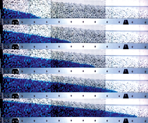
 $\gamma$ values; table 1 summarizes experiments and corresponding parameters. Sample snapshots of the current profile for Exp. 13 are shown in figure 11.
List of the experiments: (b) indicates smaller glass beads with  $d=4.0\pm 0.1\,\text {mm}$; (B) indicates larger glass beads with
 $d=15.5\pm 0.3\,\text {mm}$; (g) indicates gravel with diameter
 $d=7\unicode{x2013}15\,\text {mm}$.

Snapshots of the profiles of the current for Exp. 13. Constant inflow rate with the current advancing in natural gravels.

6.2. Experimental results and discussion
Figure 12 shows the current profile for Exp. (b)5, with a linearly increasing inflow rate. The straight dash–dotted lines are the theory, which is in very good agreement with the experimental profiles. Similar good agreement is also found for other experiments (not shown).
Profiles of the current for Exp. (b)5, small glass beads with linearly increasing inflow rate,  $\gamma =2$ and
 $X_N\propto T$. The dash–dotted straight lines are the theoretical results.

Results for the nose position of the currents are shown in figure 13(a,b) for all experiments with a waxing or constant inflow rate ( $\gamma \le 1$). The graphs show, on a bilogarithmic scale, the dependency on time of the experimental nose position compared with its theoretical counterpart, calculated for the case of high/low local Forchheimer number, depending on the regime asymptotically reached by the GC. In seven instances, the current asymptotically reaches the high local Forchheimer regime, while for the remaining two cases (Exp. (B)9 and Exp. (g)13), a progressive deceleration of the nose is observed until the low local Forchheimer number regime is reached. It is seen that the results of the theoretical models are in good agreement with the experiments, i.e. the semianalytical predictions based on the approximation well predict the asymptotic behaviour of the current nose.
Experimental nose position  $X_N$ versus time
 $T$. (a) Waning inflow rate with different values of
 $\gamma$, and (b) constant inflow rate with
 $\gamma =1$. The continuous black and dashed red lines refer to the high/low local Forchheimer number regime, with a time exponent equal to
 $(\gamma +2)/4$ (high) and
 $(\gamma +1)/3$ (low), respectively. Data are translated along the vertical for better visualization.

Figure 14(a) shows the nose position for the experiments with  $\gamma =2$, corresponding to a linearly increasing flow rate. In this case, the mathematical formulation admits an analytical solution predicting a constant nose speed. For a better comparison, a linear scale was used for both axes. After an initial adaptation, the self-similar regime clearly emerges, with experimental points aligned on a straight line, indicating a good match with theory. Figure 14(b), again using logarithmic scales, refers to waxing inflow rate tests with
 $\gamma >2$. For Exp. 6 and Exp. 11 the asymptotic high local Forchheimer number regime is well reproduced, but for the superwaxing inflow rate Exp. 16 an evident acceleration of the nose is not followed by the limit high regime, which would imply
 $X_N\propto T^{1.8}$. This phenomenon is due to the fact that the maximum flow rate of the pump was reached before self-similarity was perfected. Noteworthy, this is a strongly accelerating flow: the GC has to travel a reasonable distance from the origin before it converges to self-similarity, forgetting the initial and boundary conditions. At the same time, when the inflow rate becomes constant as the pump reaches its maximum flow rate, the profile evolves towards the characteristic of
 $\gamma =1$.
Experimental nose position  $X_N$ versus time
 $T$. (a) Waxing inflow rate with
 $\gamma =2$, and (b) waxing inflow rate with
 $\gamma >2$. Panel (a) axes are linear for stricter validation. For caption, see figure 13.

This analysis of the evolution of the regime of the current nose can be carried out by calculating the value of the local time exponent  $\omega$ (where
 $X_N\propto T^{\omega })$ as
 $\omega =T\dot {X}_N/X_N$, interpolating the experimental data
 $X_N(T)$ with a polynomial and calculating the time derivative
 $\dot {X}_N$. Figure 15 shows the time evolution of
 $\omega$ for Exp. 2 with a constant inflow rate (
 $\gamma =1$), with a lower/upper limit equal to
 $0.67/0.75$, and for Exp. 16 in superwaxing inflow rate (
 $\gamma =5.2$). For Exp. 2, after an initial adjustment,
 $\omega$ reaches a plateau around 0.75, followed by a progressive decay towards the low limit regime
 $\omega =0.67$. For Exp. 16, there is an evident acceleration with a maximum
 $\omega \approx 1.28$, followed by a decay when the pump has reached the maximum inflow rate.
Local time exponent  $\omega$ of the nose position, with
 $X_N\propto T^{\omega }$. The dashed lines are the theoretical values
 $\omega =0.75$ for
 $\bar {\zeta }\gg 1$ (upper line) and
 $\omega =0.67$ for
 $\bar {\zeta }\ll 1$ (lower line) and Exp. (b)2 with
 $\gamma =1$. The arrows indicate the axes for the two (upper and lower) lines, time increases from left to right.

7. Summary and conclusions
The present study extends the well-known problem of GC propagation in porous media to the Forchheimer regime. The starting assumptions are (i) plane GCs advancing in homogeneous porous media over an impermeable bottom under the Darcy–Forchheimer flow law; (ii) thin current warranting the lubrication approximation; (iii) lack of capillary effects; (iv) existence of a representative elementary volume even in presence of coarse media. Further, the model assumes that the fluid volume of the current varies with time according to a power function of exponent  $\gamma$, capable of simulating the dam-break condition (
 $\gamma =0$), constant, waxing and waning inflow rates.
The study adopts analytical, numerical and experimental approaches. Mathematically, the resulting nonlinear, diffusion-like governing equations in  $H(X,T)$ requires, in general, a numerical approach. However, it is possible to find certain self-similar solutions that transform the PDE describing the propagation of the current into an easily solved ODE in
 $H(\chi )$, where
 $\chi$ combines space
 $X$ and time
 $T$, eliminating the initial condition and transforming the boundary condition at the origin into an integral mass conservation of the fluid over time. The ODE numerical solution is valid in the intermediate asymptotic regime and does not require an initial condition, as a consequence of the reduction of the number of the independent variables. Specifically, self-similar solutions are obtained in the limiting conditions of a local Forchheimer number very small/large at first/zero order, respectively. As subcases, analytical solutions were obtained for
 $\gamma =0$ and for
 $\gamma =2$. This last condition is obtained either with governing equations written with a different scaling of the time, or as a limit for
 $\gamma \to 2$ of the governing equations written with the standard scaling adopted for
 $\gamma \ne 2$. The results are obviously the same. Table 2 summarizes the approaches adopted to solve the governing equations and some main results.
Summary of the methods adopted for solving the governing equations. Here  $\bar {\zeta }=(4N/X_N)\int _0^{X_N}|\partial H/\partial X|\,\text {d}X$ is the (average) local Forchheimer number,
 $\varPhi '(1)$ is the second boundary condition for the numerical integration of the governing equations admitting a self-similar solution. The solution for
 $\gamma =2$ can be also obtained as limit for
 $\gamma \to 2$ of the solution for
 $\gamma \ne 2$, see the details in the main body of the text.

The asymptotic behaviour of the self-similar solutions has been numerically verified by comparison with the numerical results of the direct integration of the full governing equations. Although the robustness of the adopted schemes suggests that the proposed solutions are capable of reproducing physical reality, experimental validation is essential.
A series of 16 experiments carried out in a channel filled with glass spheres of two different diameters and natural marble gravel allowed the recording of the temporal position of the nose and the profiles of the currents under waning, constant and waxing inflow rate. The two coefficients  $\alpha$ and
 $\beta$ were estimated for the three different porous media with a different experimental apparatus. The data analysis shows that within the limits of the uncertainties the theoretical model is in good agreement with the experimental evidence, and confirms the existence of self-similar regimes under Darcy–Forchheimer flow.
Further conclusions specific to different values of  $\gamma$ are as follows.
(i) For
$\gamma <1$ (waning inflow rate) in the high-Forchheimer-number regime, the local Forchheimer number decreases asymptotically as the average current slope slows down as $\sim T^{(\gamma -2)/2}$. This means that flows initially in the high-Forchheimer-number regime asymptotically reach the low-Forchheimer number-regime. In particular, for the dam break case ($\gamma =0$), the profile evolves from a cubic to a quadratic parabola, and the nose propagation rate goes from $\sim T^{1/2}$ to $\sim T^{1/3}$. This behaviour also applies to GC in the waxing regime, but with $\gamma <2$, i.e. GCs with decelerating nose speed.(ii) For
$\gamma =2$ (input flow rate increasing linearly with time), the problem admits a self-similar solution with a linear profile and the nose advances at constant speed. This solution is similar to that obtained for a GC of Herschel–Bulkley fluid by Di Federico et al. (Reference Di Federico, Longo, King, Chiapponi, Petrolo and Ciriello2017). The two low/high local Forchheimer number subcases fall into the general case, with some simplifications. Note that the slope of the current profile is both time-invariant and uniform, hence, the current will not change its average local Forchheimer number over time. The current midplane section is a triangle with homothetic transformation during time.(iii) For
$\gamma >2$, even if the GC is initially in the low-Forchheimer-number regime, it evolves towards the high-Forchheimer number-regime as the average slope of the profile grows over time. However, before reaching this regime, the average slope may assume such large values that the thin current model becomes inapplicable. Hence, there is an intermediate interval when both events occur, rendering the high-Forchheimer-number regime feasible.


Finally, the appendices illustrate specific aspects of the problem at hand. Appendix A illustrates different possible expressions for the pure parameter  $N$ governing the dimensionless formulations of the problem. Here
 $N$ is shown to be proportional to the intensity of the nonlinear Forchheimer correction and to the squared ratio between buoyancy and viscous forces, akin to a Grashof number. Here
 $N$ ranges normally between
 $10^{-5}$ and
 $10^{2}$ and between 2.8 and 64 in our experiments.
Appendix B presents a simple expression for the average slope of the current.
In Appendix C the self-similar solution approach is briefly derived and a self-similar solution of the general case is sketched, with the expansion in series of functions where the fundamental solution corresponds to the low local Forchheimer number case at first order. The coefficients of the series are powers of time calculated to guarantee the invariance of the additional terms in the same parameter of transformations that admits the self-similarity of the fundamental solution. The convergence condition of the function series indicates that, at each order, the solution is valid if  $T\ll T_c\equiv N^{3/(2-\gamma )}$ when
 $\gamma <2$ and
 $T\gg T_c$ when
 $\gamma >2$.
 $T_c$ is named critical time. For
 $\gamma =2$ the value of
 $T_c\to \infty$ and this suggests that the self-similar solution is possible for the complete governing equations, as actually verified.
Future developments include the extension of the Darcy–Forchheimer flow law to infinite radial geometry, finite domains and non-Newtonian flows.
Funding
This work was supported in part by Università di Bologna RFO 2022 grant awarded to Vittorio Di Federico. S.L. acknowledges that this work was supported by a Project funded under the National Recovery and Resilience Plan (NRRP), Mission 4 Component 2 Investment 1.5 – Call for tender no. 3277 of 30/12/2021 of Italian Ministry of University and Research funded by the European Union – NextGenerationEU. Project code ECS00000033, Concession Decree no. 1052 of 23/06/2022 adopted by the Italian Ministry of University and Research, CUP D93C22000460001, ‘Ecosystem for Sustainable Transition in Emilia-Romagna’ (Ecosister), Spoke 4. The numerical information is provided in the figures produced by solving the equations in the paper. Results of the experiments are available from the authors on request.
Declaration of interests
The authors report no conflict of interest.
Appendix A. The dimensionless parameter $N$

The pure number  $N$ may be expressed as a function of well-known dimensionless parameters in fluid mechanics (see e.g. Massey Reference Massey1971; Longo Reference Longo2021a). Multiplying and dividing (2.15) by
 $u_0^2 d^2$, where
 $u_0$ is the velocity scale defined in (2.11a–c) and
 $d$ the characteristic length (diameter) of the porous medium, yields
 \begin{equation} N=\dfrac{Re\,Fo\,Da}{Fr_d^2}, \end{equation}
where  $Re=(\rho u_0 d)/\mu$ is the classical pore-scale Reynolds number, equal to the ratio between convective inertial forces and viscous forces,
 $Fo=(\rho \beta k u_0)/\mu$ is the Forchheimer number, a modified version of the Reynolds number expressing the ratio between nonlinear effects associated with the Forchheimer correction to Darcy's law and viscous effects,
 $Da=k/d^2$ is the Darcy number, representing the relative effect of the permeability of the medium versus its cross-sectional area and
 $Fr_d=u_0/\sqrt {(\Delta \rho /{\rho })gd}$ a pore-scale densimetric Froude number, equal to the square root of the ratio between convective inertia and buoyancy.
Note that (A1) can be recast as
 \begin{equation} N=\dfrac{d^2}{h_0^2}\dfrac{Re'\,Fo\,Da}{Fr_d^{'2}} \end{equation}
upon redefining the pore-scale Reynolds and densimetric Froude numbers via their large-scale counterparts  $Re'=(\rho u_0 h_0)/\mu$,
 $Fr'_d=u_0/\sqrt {(\Delta \rho /\rho )g h_0}$, where the height of the porous domain
 $h_0$ is taken as the relevant length scale in lieu of the characteristic pore diameter
 $d$.
A third, and more parsimonious, option to represent  $N$ is writing
 \begin{equation} N=\dfrac{Re^{''}\,Fo}{Fr^{''2}_d}, \end{equation}
where the alternative definitions of the Reynolds number  $Re^{''}=(\rho u_0 \sqrt {k})/\mu$ and densimetric Froude number
 $Fr^{''}_d=u_0/\sqrt {(\Delta \rho /\rho )g \sqrt {k}}$ incorporate
 $\sqrt {k}$ as the relevant length scale.
Finally, an alternative expression of (A3) that dispenses with the Forchheimer number is
 \begin{equation} N=C_D\dfrac{Re^{''2}}{Fr^{''2}_d}\propto \left(\frac{\text{buoyancy forces}}{\text{viscous forces}}\right)^2, \end{equation}
where  $C_D$ is the dimensionless form-drag coefficient defined in (2.2). Equation (A4) demonstrates that essentially
 $N$ is a Grashof number modulated by the dimensionless factor
 $C_D$ expressing the intensity of the Forchheimer nonlinear correction to Darcy's law. In fact, the Grashof number is usually expressed as
 \begin{equation} Gr=\dfrac{\Delta\rho}{\rho}\dfrac{g l^3}{\nu^2}, \end{equation}
where  $l$ is a length scale. Here, the density variations are not linked to temperature effects as usual, but to the presence of two fluids, the intruding and the ambient, having a density difference
 $\Delta \rho$. When
 $l$ is taken to be equal to
 $\sqrt {k}$ and using (2.2), it is seen that
 $N=C_D Gr$.
To derive values of  $N$ typical of laboratory or field applications, consider first a
 $\Delta \rho /\rho$ in the range
 $0.1-0.9$, the two bounds being representative of the Boussinesq or non-Boussinesq regime, respectively. Then, one can typically take for the fluid properties those of water at
 $10\,^{\circ }\text {C}$,
 $\rho =999.7\,\text {kg}\,\text {m}^{-3}$ and
 $\mu =1.337\times 10^{-3}\,\text {Pa}\,\text {s}$. As
 $\beta$ and
 $k$ are correlated (Lenci et al. Reference Lenci, Zeighami and Di Federico2022), ranges of values of
 $k$ and
 $\beta$ are conveniently deduced from Sidiropoulou, Moutsopoulos & Tsihrintzis (Reference Sidiropoulou, Moutsopoulos and Tsihrintzis2007), who report
 $k$ and
 $b$ pairs (
 $\beta =b/g$) as a consequence of (2.1) and (2.3) measured in different experiments. There, we select the experiment on sand media with the lowest
 $k$ and that on gravel media with the highest
 $k$ as ideally representative of the two approximate regimes of low and high local Forchheimer number. The corresponding parameter values are
 $k=2.1\times 10^{-10}\,\text {m}^2$,
 $\beta =759\,\text {m}^{-1}$ for sand (their data set
 $\#77$), and
 $k=2.04\times 10^{-6}\,\text {m}^2$,
 $\beta =50\,\text {m}^{-1}$ for gravel (their data set
 $\#72$). These two pairs yield
 $N=1.84\times 10^{-5}$ or
 $N=1.65\times 10^{-4}$ for sand and
 $N=3.49$ or
 $N=31.4$ for gravel, depending whether
 $\Delta \rho /\rho =0.1$ or
 $\Delta \rho /\rho =0.9$. Hence the potential range of
 $N$ is very large, i.e. approximately
 $N\in [10^{-5},10^{2}]$ for fluids with a kinematic viscosity close to water, and includes the case
 $N=1$ entailing roughly a balance between buoyancy and viscous forces. Most fluids have a kinematic viscosity higher than water, so in these cases the lower limit decreases below
 $10^{-5}$; it can (modestly) increase above
 $10^{2}$ for those few fluids having kinematic viscosity lower than water. In the experiments described in § 6, the value of
 $N$ ranges between 2.8 and 64.
Appendix B. An alternative expression for the average slope of the current
An alternative, approximate expression for the slope of the GC is derived here, to dispense with the evaluation of the average value of the first derivative of the shape function,  $\overline {\textrm {d}\varPhi /\textrm {d}\chi }$, in (3.13a,b) and (3.30a,b). Approximating the current with a prism of longitudinal triangular cross-section of length
 $x_N$ and height
 $x_N \tan \varphi$, where
 $\tan \varphi$ is the slope, the current volume per unit width is
 $\frac {1}{2}x^2_N \tan \varphi =qt^\gamma /\phi$, or
 $\frac {1}{2}X^2_N \tan \varphi =T^\gamma$ in dimensionless form, yielding
 $\tan \varphi =|\partial H/\partial X|=(2T^\gamma )/X^2_N$. This gives for the slope of the current
 \begin{equation} S\equiv\left|\frac{\partial H}{\partial X}\right|=\frac{2}{\xi^2_N}T^{({\gamma-2})/{3}}, \quad S\equiv \left|\frac{\partial H}{\partial X}\right|=\frac{2}{\xi^2_N}T^{({\gamma-2})/{2}} \end{equation}
for the low- and high-Forchheimer case, respectively.
The approximation is exact if  $\gamma =2$ and, in this case, the current profile is linear, but the slope must be computed with the same approach adopted for (3.16)–(3.31).
Appendix C. The self-similar solution approach and the solution expanding in series of functions
We first consider the reduced problem in the limit  $\zeta \ll 1$, see (3.3) with the constraints (2.14a,b). The transformation group leaving the problem invariant can be obtained by assuming a possible structure as
 $X'=aX,T'=bT,H'=cH$, where the prime refers to the variable in a new space and
 $a,b,c$ are real coefficients. Substituting into the governing equations yields
 \begin{equation} \frac{\partial H'}{\partial T'}=N\frac{\partial}{\partial X'}\left(H'\frac{\partial H'}{\partial X'}\right)\to \frac{c}{b}\frac{\partial H}{\partial T}=N\dfrac{c^2}{b^2}\frac{\partial}{\partial X}\left(H\frac{\partial H}{\partial X}\right), \end{equation}
and
 \begin{equation} \int_0^{\infty}H'\,\text{d}\kern0.7pt X'=T'^{\gamma}\to ac\int_0^{\infty}H\,\text{d}\kern0.7pt X=b^{\gamma}T^{\gamma}. \end{equation}
The invariance requires that
 \begin{equation} \dfrac{c}{b}=\dfrac{c^2}{b^2},\quad ac=b^{\gamma}, \end{equation}
which admits the solution
 \begin{equation} b=a^{F_2},c=a^{F_1},\quad \text{with}\ F_1=\dfrac{2\gamma-1}{\gamma+1},F_2=2-F_1. \end{equation}
That means that the group of transformation for the single-parameter  $a$ reads
 \begin{equation} X'=aX,\quad T'=a^{F_2}T,\quad H'=a^{F_1}H. \end{equation}
Assuming time as fundamental variable, the dimensions of  $X$ and
 $H$ are
 $X\sim T^{-r}$ and
 $H\sim T^{-s}$ with
 $r=1/F_2$ and
 $s=F_1/F_2$. According to the principle of covariance, the solution of the governing equations can be expressed as
 $f(HT^{-s},XT^{-r})=0$. For progress, we can assume that
 $H=T^sf(XT^{-r})$. This is the conceptualization that leads to the governing equations represented by (3.8)–(3.9).
Looking at the full governing equations ((2.13)–(2.14a,b)), it results that a self-similar solution of the general case is possible only if within the same group (C5a{–}c) the term
 \begin{equation} \sqrt{1+N\left|\frac{\partial H}{\partial X}\right|}, \end{equation}
is invariant, equivalent to saying that  $H$ and
 $X$ must have the same time dependence otherwise their ratio cannot match the units, already invariant under any transformation. This holds true only for
 $\gamma =2$ since
 \begin{equation} N'\frac{\partial H'}{\partial X'}=N\dfrac{a^{F_1}}{a}\frac{\partial H}{\partial X}\to N'=N\quad \text{if}\ F_1=1. \end{equation}
The general case can be approached by assuming that  $N$ is a further variable, instead of a parameter, and extending the group of transformations,
 \begin{equation} X'=aX,\quad T'=a^{F_2}T,\quad H'=a^{F_1}H,\quad N'=a^{1-F_1}N. \end{equation}
Assuming again  $T$ as fundamental variable, we have now three invariants within the transformation, namely
 $XT^{-r}$,
 $HT^{-s}$,
 $NT^{-m}$, where
 $m$ is computed imposing the invariance of
 \begin{equation} \dfrac{N'}{T'^m}=\dfrac{a^{1-F_1}}{a^{mF_2}}\dfrac{N}{T^,}\to m=\dfrac{1-F_1}{F_2}\equiv \dfrac{\gamma-2}{3}. \end{equation}
The formal solution of the governing equations can be now expressed as
 \begin{equation} H=T^sg(XT^{{-}r},NT^{{-}m})\quad\text{or}\quad H=T^sg(\eta,\sigma),\quad \eta=XT^{{-}r},\quad \sigma=NT^{{-}m}. \end{equation}
We do not have further information on the structure of the function  $g$. For progress, we can expand the function about
 $\sigma = 0$ for small values of
 $\sigma$,
 \begin{equation} g(\eta,\sigma)=\left.g\right|_{(\eta,0)}+\left.\dfrac{\partial g}{\partial \sigma}\right|_{(\eta,0)}\sigma+O(\sigma^2). \end{equation}
Following the same procedure in Di Federico et al. (Reference Di Federico, Longo, King, Chiapponi, Petrolo and Ciriello2017) as detailed in Longo (Reference Longo2021b), we look for a perturbation of the fundamental first-order solution with an expansion in the regime  $\sigma \equiv NT^{(\gamma -2)/3}\ll 1$,
 \begin{gather} H(X,T)=\xi_N^2 T^{(2\gamma-1)/3} [\varPhi_0(\chi)+\sigma\varPhi_1(\chi)+\cdots], \end{gather}
 \begin{gather} X=\xi T^{{(\gamma+1})/3}(1+\sigma X_1+\cdots), \end{gather}
where  $\varPhi _0(\chi )$ and
 $\xi _N$ are given by the first-order solution, and
 $X_1$ is a constant to be evaluated. The condition
 $\sigma \ll 1$ requires that (i) for
 $\gamma <2$,
 $T\ll T_c\equiv N^{3/(2-\gamma )}$; and (ii) for
 $\gamma >2$,
 $T\gg T_c$,
 $T_c$ being the critical time. For
 $\gamma =2$ the critical time becomes infinite and this corresponds to a self-similar solution for the full governing equations, without need of approximations, but requiring a different scaling of the variables as detailed in § 4.
Substituting (C12)–(C13) in (2.13)–(2.14a,b), at  $O(1)$ we recover the fundamental solution, with
 $\varPhi _0$ coincident with the solution of the governing equations (3.8) plus the constraints. The result at
 $O(\sigma )$ is
 \begin{equation} N\left(\varPhi_1'\varPhi_0+\varPhi_1\varPhi_0'\right)'+\chi\varPhi_1'-(\gamma-1)\varPhi_1=0, \end{equation}
which is a quasilinear ODE where  $\varPhi _0$ is a forcing term, and that can be integrated with a further boundary condition at the nose of the current. The integral constraint (2.14a,b) becomes
 \begin{equation} \xi_N(1+\sigma X_1+\ldots)\int_0^{1+\sigma X_1+\ldots}[\phi_0(\chi)+\sigma\varPhi_1(\chi)+\ldots]\,\text{d}\chi=1, \end{equation}
which at  $O(\sigma )$ yields
 \begin{equation} X_1={-}\dfrac{\int_0^1\varPhi_1(\chi)\,\text{d}\chi}{\int_0^1\varPhi_0(\chi)\,\text{d}\chi}. \end{equation}


 Open access

