1 Introduction
Intense nearly axisymmetric vortices often develop in geophysical flows, tornadoes or hurricanes in the atmosphere, while in the ocean, the sea surface height variability appears to be dominated by westward-propagating mesoscale eddies throughout most of the World Ocean (Chelton et al. Reference Chelton, Schlax and Samelson2011). In order to understand their characteristics, it is instructive to model such objects as isolated structures (see Persing et al. Reference Persing, Montgomery, Smith and McWilliams2015; Oruba, Davidson & Dormy Reference Oruba, Davidson and Dormy2017, and references therein). Their natural embedding inside a cylindrical domain introduces the need for an artificial outer circular sidewall boundary. Although no-slip boundaries could be contemplated, they introduce additional friction and so nowadays other boundary conditions are usually considered. Whatever the model, boundary layers are important (see, e.g., Smith & Montgomery Reference Smith and Montgomery2010).
Williams (Reference Williams1968) was the first to suggest removing some frictional constraints associated with the sidewalls in the numerical models, in order to more faithfully mimic the unbounded physical domain. Viscous friction was then only retained at the bottom boundary, as in atmospheric flows. Since then, stress-free sidewalls, at which the angular velocity gradient vanishes, have been used in several numerical studies (see, e.g., Read Reference Read1986a ,Reference Read b ), while matching to an external azimuthal flow corresponding to an axial line vortex (no viscous force) is sometimes preferred (see, e.g., Montgomery et al. Reference Montgomery, Snell and Yang2001).
Here, we investigate the effects of a stress-free sidewall on such flows in the small-Ekman-number
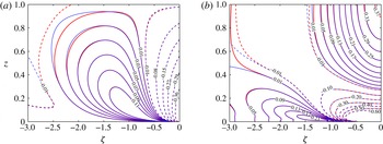
 $E$
limit (see (1.1)). Specifically, we consider the classical linear spin-down problem (see, e.g., Greenspan & Howard (Reference Greenspan and Howard1963) and the review of Benton & Clark (Reference Benton and Clark1974); for nonlinear studies see, e.g., Wedemeyer (Reference Wedemeyer1964), Hyun et al. (Reference Hyun, Leslie, Fowlis and Warn-Varnas1983) and the review of Duck & Foster (Reference Duck and Foster2001)) in a domain with a no-slip boundary at the bottom but modified by the presence of stress-free sidewall and top boundaries. Like Greenspan & Howard (Reference Greenspan and Howard1963), we find that during the early stages, the mainstream spin-down exterior to all boundary layers is characterised by an angular velocity that is spatially constant but decays exponentially in time just as in an infinite (unbounded) plane layer (see § 1.1). However, on a somewhat longer time scale, the quasi-geostrophic angular velocity develops a radial (non-constant) structure dependent on the jump condition across the Stewartson (Reference Stewartson1957)
 $E^{1/3}$
sidewall shear layer. In the rigid-boundary case studied by Greenspan & Howard (Reference Greenspan and Howard1963), that shear layer is passive and the quasi-geostrophic angular velocity simply vanishes at the mainstream boundary. This may be interpreted as a retrograde torque at the outer boundary which enhances the decay of the angular velocity with increasing radius. In our stress-free boundary case, the torque at the true boundary certainly vanishes. Nevertheless, the return meridional flow in the
 $E^{1/3}$
layer is necessarily opposite to that needed to achieve spin-down in the mainstream. Therefore, from that point of view, it is perhaps not surprising to find that the outer boundary essentially opposes spin-down rather than enhancing it. This notion is made quantitatively precise in § 5 by identifying the decay rate of the dominant mode as time tends to infinity. For the cases of stress-free and rigid boundaries at finite radius
 $L$
, their magnitudes are less than and respectively greater than the value for an unbounded fluid
 $L\rightarrow \infty$
(see (5.1) and (5.2)). Essentially, the
 $E^{1/3}$
layer is no longer passive but completely alters the effective mainstream boundary condition. Consequently, the mainstream flow experiences a prograde boundary torque proportional to the quasi-geostrophic angular velocity there. In turn, that causes the angular velocity to increase (rather than decrease) outwards (see (1.8)). This was an unexpected finding, although with hindsight it is easily explained.
In application to unbounded geophysical flows such as hurricanes, the counterintuitive consequences of the unnatural impermeable sidewall boundary condition do not occur. An understanding of why they happen in the idealised model is essential for improving future numerical models. This is one of our main conclusions upon which we expand in the discussion (§ 5).
1.1 Our variant of the Greenspan and Howard problem
Here, we describe in more detail our variant of the Greenspan & Howard (Reference Greenspan and Howard1963) model. Relative to cylindrical polar coordinates,
 $(r^{\star },\unicode[STIX]{x1D703}^{\star },z^{\star })$
, we consider a cylindrical container of height
 $H$
and radius
 $L$
rotating rapidly with angular velocity
 $\unicode[STIX]{x1D734}$
about its axis of symmetry. The container is filled with constant-density fluid of viscosity
 $\unicode[STIX]{x1D708}$
, which initially at time
 $t^{\star }=0$
rotates rigidly with the slightly different angular velocity
 $(1+Ro)\unicode[STIX]{x1D734}$
, in which the Rossby number
 $Ro$
is sufficiently small for linear theory to apply. The top boundary (
 $r^{\star }<L$
,
 $z^{\star }=H$
) and the sidewall (
 $r^{\star }=L$
,
 $0<z^{\star }<H$
) are impermeable and stress-free. The lower boundary (
 $r^{\star }<L$
,
 $z^{\star }=0$
) is rigid. For that reason alone, the initial state of rigid rotation
 $(1+Ro)\unicode[STIX]{x1D734}$
of the fluid cannot persist, and the fluid spins down to the final state of rigid rotation
 $\unicode[STIX]{x1D734}$
of the container as
 $t^{\star }\rightarrow \infty$
.
The rapid rotation of the system is measured by the small Ekman number
 $$\begin{eqnarray}E=\unicode[STIX]{x1D708}/(H^{2}\unicode[STIX]{x1D6FA})\ll 1.\end{eqnarray}$$
In this limit, it is known that for the Greenspan & Howard (Reference Greenspan and Howard1963) rigid-sidewall problem, linear theory is restricted to the range
 $Ro\ll E^{1/4}$
(see Duck & Foster Reference Duck and Foster2001, p. 235). We anticipate that this restriction also applies to our stress-free sidewall case.
On very short time scales, shear layers form adjacent to all boundaries of width
 $$\begin{eqnarray}\unicode[STIX]{x1D6FF}^{\star }(t^{\star })=(\unicode[STIX]{x1D708}t^{\star })^{1/2}=H(E\unicode[STIX]{x1D6FA}t^{\star })^{1/2}\end{eqnarray}$$
due to viscous diffusion. On the short inertial wave time scale
 $t^{\ast }=1/\unicode[STIX]{x1D6FA}$
, a quasi-steady Ekman layer of width
 $\unicode[STIX]{x1D6FF}_{E}^{\star }=(\unicode[STIX]{x1D708}/\unicode[STIX]{x1D6FA})^{1/2}=E^{1/2}H$
forms adjacent to the lower boundary
 $z^{\star }=0$
. Various inertial waves and quasi-geostrophic (
 $z^{\star }$
-independent; QG) motions exterior to all boundary layers are generated in the mainstream, which decay primarily due to the ensuing Ekman suction into (or blowing out of) the Ekman layer (see Zhang & Liao (Reference Zhang and Liao2008), and the references therein, particularly Kerswell & Barenghi (Reference Kerswell and Barenghi1995)). Our numerical results generally show that motion is soon dominated by the QG flow which spins down on the longer time scale
 $H/(\unicode[STIX]{x1D708}\unicode[STIX]{x1D6FA})^{1/2}=E^{-1/2}/\unicode[STIX]{x1D6FA}$
. Indeed, relative to the frame rotating with angular velocity
 $\unicode[STIX]{x1D734}$
, the cylindrical components of the mainstream velocity are simply
 $$\begin{eqnarray}(\overline{\breve{u}^{\star }},\overline{\breve{v}^{\star }},\overline{\breve{w}^{\star }})=Ro\unicode[STIX]{x1D6FA}\unicode[STIX]{x1D705}({\textstyle \frac{1}{2}}\unicode[STIX]{x1D70E}E^{1/2}r^{\star },r^{\star },\unicode[STIX]{x1D70E}E^{1/2}(H-z^{\star }))\exp (-\unicode[STIX]{x1D70E}E^{1/2}\unicode[STIX]{x1D6FA}t^{\star }),\end{eqnarray}$$
as determined by the solution to the initial value problem for a layer of unbounded horizontal extent outlined in appendix A and previously considered by Greenspan & Howard (Reference Greenspan and Howard1963). The purpose of appendix A is to extend Greenspan & Howard’s
 $\unicode[STIX]{x1D705}\approx 1$
,
 $\unicode[STIX]{x1D70E}\approx 1$
results to determine their more precise forms (A 5b
) and (A 8a
) respectively. They have expansions
 $$\begin{eqnarray}\unicode[STIX]{x1D705}=1+{\textstyle \frac{1}{4}}E^{1/2}+O(E),\quad \unicode[STIX]{x1D70E}=1+{\textstyle \frac{3}{4}}E^{1/2}+O(E)\end{eqnarray}$$
(see (A 9a
) and (A 8b
) respectively), which prove useful when comparing our numerical results at finite
 $E$
with our asymptotic predictions. The spin-down motion (1.3a
) is characterised by a fluid flux inside the Ekman layer towards the axis, which is blown out into the mainstream with velocity
 $\overline{\breve{w}^{\star }}|_{z^{\star }=0}=Ro\unicode[STIX]{x1D6FA}\unicode[STIX]{x1D705}\unicode[STIX]{x1D70E}E^{1/2}H$
. This generates a radial outflow in the mainstream of magnitude
 $\overline{\breve{u}^{\star }}|_{z^{\star }>0}=Ro\unicode[STIX]{x1D6FA}\unicode[STIX]{x1D705}\unicode[STIX]{x1D70E}E^{1/2}Hr^{\star }/2$
, which by conservation of angular momentum causes the angular velocity decay
 $$\begin{eqnarray}\overline{\breve{\unicode[STIX]{x1D714}}^{\star }}(t^{\star })=\overline{\breve{v}^{\star }}/r^{\star }=Ro\unicode[STIX]{x1D6FA}\unicode[STIX]{x1D705}\exp (-\unicode[STIX]{x1D70E}E^{1/2}\unicode[STIX]{x1D6FA}t^{\star }).\end{eqnarray}$$
The mainstream outflow is blocked by the outer boundary
 $r^{\star }=L$
, where a quasi-steady Stewartson (Reference Stewartson1957) sidewall layer of width
 $\unicode[STIX]{x1D6FF}_{S}^{\star }=E^{1/3}H$
forms (see Barcilon Reference Barcilon1968) on the time scale
 $t^{\ast }=E^{-1/3}/\unicode[STIX]{x1D6FA}$
, long compared with the Ekman layer time scale
 $1/\unicode[STIX]{x1D6FA}$
but short compared with the spin-down time
 $E^{-1/2}/\unicode[STIX]{x1D6FA}$
. Following the formation of the
 $E^{1/3}$
Stewartson layer, an ever-thickening QG shear layer emerges of width
 $\unicode[STIX]{x1D6FF}^{\star }(t^{\star })=H(E\unicode[STIX]{x1D6FA}t^{\star })^{1/2}$
(see (1.2)). On the spin-down time scale
 $E^{-1/2}/\unicode[STIX]{x1D6FA}$
, it has width
 $E^{1/4}H$
, which prompted Greenspan & Howard (Reference Greenspan and Howard1963) to refer to it as an
 $E^{1/4}$
layer. The implied link with the static
 $E^{1/4}$
Stewartson layer is misleading as the dynamical balances are different and there are no persistent (quasi-static)
 $E^{1/4}$
layers in the spin-down problem (see also the discussion below (2.13) and in § 5).
Following the establishment of the
 $E^{1/3}$
layer (i.e.
 $E^{1/3}\unicode[STIX]{x1D6FA}t^{\star }\gg 1$
), the QG shear layer thickens:
 $\unicode[STIX]{x1D6FF}^{\star }(t^{\star })=H(E\unicode[STIX]{x1D6FA}t^{\star })^{1/2}$
. This modifies the spin-down profile (1.4) both spatially and temporally on the longer lateral diffusion time
 $L^{2}/\unicode[STIX]{x1D708}=\ell ^{2}E^{-1}/\unicode[STIX]{x1D6FA}$
, where
 $$\begin{eqnarray}\ell =L/H\end{eqnarray}$$
is the container aspect ratio. This suggests a two-time-scale approach (see, e.g., Hinch Reference Hinch1991, ch. 7) in which (1.4) is modulated by a factor
 $\overline{{\unicode[STIX]{x1D714}\unicode[STIX]{x0030A}}}(r^{\star }/H,E\unicode[STIX]{x1D6FA}t^{\star })$
, so taking the form
 $$\begin{eqnarray}\overline{\breve{\unicode[STIX]{x1D714}}^{\star }}(r^{\star },t^{\star })=Ro\unicode[STIX]{x1D6FA}\unicode[STIX]{x1D705}\overline{{\unicode[STIX]{x1D714}\unicode[STIX]{x0030A}}}(r^{\star }/H,E\unicode[STIX]{x1D6FA}t^{\star })\exp (-\unicode[STIX]{x1D70E}E^{1/2}\unicode[STIX]{x1D6FA}t^{\star }).\end{eqnarray}$$
Matching with the short-time solution (1.4), as
 $E\unicode[STIX]{x1D6FA}t^{\star }\downarrow 0$
, is achieved by demanding that initially
 $$\begin{eqnarray}\overline{{\unicode[STIX]{x1D714}\unicode[STIX]{x0030A}}}(r^{\star }/H,0)=1.\end{eqnarray}$$
The outer
 $r^{\star }=L$
boundary condition on the QG mainstream flow depends on the jump conditions across the
 $E^{1/3}$
sidewall layer.
For the rigid outer boundary considered by Greenspan & Howard (Reference Greenspan and Howard1963), the jump in azimuthal velocity across the
 $E^{1/3}$
layer is negligible and so the outer boundary condition on the mainstream angular velocity is simply
 $\overline{\breve{\unicode[STIX]{x1D714}}^{\star }}(L,t^{\star })=0$
. It causes the early rigid rotation profile (1.4) to be further eroded to zero through lateral diffusion inwards from the outer boundary. For our stress-free outer boundary, consideration of the
 $E^{1/3}$
layer shows that the boundary condition on the angular velocity in the mainstream exterior to it (i.e.
 $r^{\ast }\uparrow L$
) is different, of mixed type, taking the Robin boundary condition form
 $$\begin{eqnarray}\frac{\unicode[STIX]{x2202}\overline{\breve{\unicode[STIX]{x1D714}}^{\star }}}{\unicode[STIX]{x2202}r^{\star }}=\unicode[STIX]{x1D6FC}{\displaystyle \frac{\overline{\breve{\unicode[STIX]{x1D714}}^{\star }}}{H}}\quad \text{at }r^{\star }=L.\end{eqnarray}$$
Here,
 $\unicode[STIX]{x1D6FC}$
is a function of
 $E$
alone determined by the nature of the
 $E^{1/3}$
layer, which itself is largely insensitive to the value of
 $L$
, while
 $2\unicode[STIX]{x03C0}HL^{3}(\unicode[STIX]{x1D70C}\unicode[STIX]{x1D708})\unicode[STIX]{x2202}\overline{\breve{\unicode[STIX]{x1D714}}^{\star }}/\unicode[STIX]{x2202}r^{\star }|_{r^{\star }=L}$
(viscosity
 $\unicode[STIX]{x1D70C}\unicode[STIX]{x1D708}$
) is the total outer (mainstream) boundary torque on the QG mainstream flow (see also (3.4)). The long-time behaviour of the solution has the functional form
 $$\begin{eqnarray}\overline{{\unicode[STIX]{x1D714}\unicode[STIX]{x0030A}}}\approx \overline{\unicode[STIX]{x1D714}}(r^{\star }/H)\exp (k^{2}\ell ^{-2}E\unicode[STIX]{x1D6FA}t^{\star }),\end{eqnarray}$$
as
 $\ell ^{-2}E\unicode[STIX]{x1D6FA}t^{\star }\rightarrow \infty$
. Unlike
 $\unicode[STIX]{x1D6FC}$
in (1.8), the constant
 $k$
is a function of both
 $E$
(via
 $\unicode[STIX]{x1D6FC}$
) and
 $\ell$
.
The main point that we wish to stress is that whereas (1.3) defines the mainstream eigensolution on the spin-down time
 $E^{-1/2}/\unicode[STIX]{x1D6FA}$
with growth rate
 $-\unicode[STIX]{x1D70E}E^{1/2}\unicode[STIX]{x1D6FA}$
, that solution evolves over the lateral diffusion time scale
 $\ell ^{2}E^{-1}/\unicode[STIX]{x1D6FA}$
and asymptotes to the form
 $$\begin{eqnarray}\overline{\breve{\unicode[STIX]{x1D714}}^{\star }}\approx Ro\unicode[STIX]{x1D6FA}\unicode[STIX]{x1D705}\overline{\unicode[STIX]{x1D714}}(r^{\star }/H)\exp (-qE\unicode[STIX]{x1D6FA}t^{\star }),\quad q=\unicode[STIX]{x1D70E}E^{-1/2}-k^{2}\ell ^{-2},\end{eqnarray}$$
with the different growth rate
 $-qE\unicode[STIX]{x1D6FA}$
and non-constant radial profile proportional to
 $\overline{\unicode[STIX]{x1D714}}(r^{\star }/H)$
. Remarkably, the stress-free outer boundary actually hinders the spin-down, as evidenced by the positive growth rate
 $k^{2}\ell ^{-2}E\unicode[STIX]{x1D6FA}$
of
 $\overline{{\unicode[STIX]{x1D714}\unicode[STIX]{x0030A}}}$
(see (1.9)). The phenomenon can be traced to the mainstream boundary torque proportional to
 $\unicode[STIX]{x2202}\overline{\breve{\unicode[STIX]{x1D714}}^{\star }}/\unicode[STIX]{x2202}r^{\star }|_{r^{\star }=L}$
determined by (1.8) with
 $\unicode[STIX]{x1D6FC}>0$
. This long-time behaviour is very different from that for the case of a rigid outer boundary, for which the corresponding form for
 $\overline{{\unicode[STIX]{x1D714}\unicode[STIX]{x0030A}}}(r^{\star }/H,E\unicode[STIX]{x1D6FA}t^{\star })$
decays (see the
 $n=1$
term of (3.8a
)) rather than growing exponentially. The striking contrast made in our discussion (§ 5) between (5.1) and (5.2), which incorporate these results, highlights the central theme of our paper.
1.2 Outline
Our notation is complicated and is best outlined in general terms at the outset. Our basic variables, like the angular velocity, are identified by the breve accent
 $\breve{~}$
. Only variables with a superscript star
 $^{\star }$
are dimensional; otherwise they are dimensionless. Azimuthal QG flows independent of
 $z^{\ast }$
are identified by an overline
 $^{\overline{~}}$
. All these notations were introduced in § 1.1. There the mathring accent
 $^{\circ }$
was also introduced in the restricted sense of mainstream QG flows, being the amplitude that remains after the spin-down decay factor
 $\exp (-\unicode[STIX]{x1D70E}E^{1/2}\unicode[STIX]{x1D6FA}t^{\star })$
is removed (see (1.6)). Below, we will however use it in the general sense (see (2.7a
)), which includes the mainstream QG part together with the Ekman layer contribution denoted by the tilde
 $\widetilde{~}$
(see (2.10)). The final eigensolution that emerges as
 $t^{\star }\rightarrow \infty$
, like the QG form (1.10) with the decay factor
 $\exp (-qE\unicode[STIX]{x1D6FA}t^{\star })$
, is otherwise without accents (see (2.29)).
We formulate the transient flow problem in its entirety in § 2. We outline the basic properties of the Ekman layer together with its consequences for the QG flow in § 2.1, in particular the QG momentum equation (2.13) governing
 $\overline{{\unicode[STIX]{x1D714}\unicode[STIX]{x0030A}}}$
and its relation (2.20a
) to the
 $z^{\star }$
average
 $\langle {\unicode[STIX]{x1D714}\unicode[STIX]{x0030A}}\rangle$
. They differ by a small amount due to the angular momentum deficit in the Ekman layer. Although the difference is small, we find that our comparisons with the numerics and asymptotics are improved by use of (2.20a
). We consider the eigenvalue problem for the final decay of the QG flow (1.10a
) in § 2.2 from an asymptotic point of view on the basis that the eigenvalue
 $k$
in (1.10b
), related to
 $\unicode[STIX]{x1D6FC}$
in (1.8), is known. Then, in § 2.3, we report results from direct numerical simulations, which confirm that the solution approaches the proposed asymptotic form. In § 2.4, we identify the shape and decay rate but not the amplitude of the eigensolution, again using numerical methods.
The transient evolution from the classical spin-down mainstream flow (1.3) to the final decay mode (1.10) (or more specifically (5.1)) is of particular interest. Therefore, in § 3, we solve the angular momentum equation (2.13) for
 $\overline{{\unicode[STIX]{x1D714}\unicode[STIX]{x0030A}}}$
subject to the initial condition (1.7) on the basis that
 $\unicode[STIX]{x1D6FC}$
in the boundary condition (1.8) is known. The numerical solution is described in § 3.1, while a power series solution valid for short times is described in § 3.2, which notably is valid on the spin-down time scale
 $E^{-1/2}/\unicode[STIX]{x1D6FA}$
when the shear-layer width is
 $E^{1/4}H$
. On that time scale, it provides our analogue of the rigid-boundary solution (Greenspan & Howard Reference Greenspan and Howard1963, equation (6.3)). Indeed, our power series is informative on much of the lateral diffusion time scale
 $\ell ^{2}E^{-1}/\unicode[STIX]{x1D6FA}$
and even provides a good approximation to
 $\overline{{\unicode[STIX]{x1D714}\unicode[STIX]{x0030A}}}$
at the outer boundary until the final asymptotic behaviour is clearly evident.
For a complete understanding of the transient evolution together with the final decay mode, we need a theory for
 $\unicode[STIX]{x1D6FC}$
. To that end, in § 4, we formulate the boundary layer equations for the
 $E^{1/3}$
layer correct not simply to leading order but to
 $O(E^{1/6})$
. We study the leading-order problem asymptotically in § 4.1.1 in the spirit of Stewartson (Reference Stewartson1957). As the solution is singular near the bottom outside corner at
 $(r^{\star },z^{\star })=(L,0)$
, there it is best expressed in a similarity form, which we provide and expand upon in § 4.1.2. Unfortunately, this leading-order solution contains no QG part. To extract the QG part, we continue in § 4.1.3 to
 $O(E^{1/6})$
, at which the singularity forces a
 $\ln E$
type dependence in the asymptotic value (4.27) of
 $\unicode[STIX]{x1D6FC}$
. As the numerical value of
 $E$
needed for the applicability of the asymptotic theory is minute, we cannot directly compare asymptotic and numerical results. To overcome this obstacle, we study in § 4.2 the numerical solution of the sidewall boundary layer equations (4.3), containing the parameter
 $\unicode[STIX]{x1D700}\equiv E^{1/6}$
explicitly at fixed
 $E$
. Their numerical solution determines
 $\unicode[STIX]{x1D6FC}$
, which we find to agree with that predicted by the full numerical eigensolution. In summary, we are unable to solve numerically the complete governing equations (2.4) at values of
 $E$
small enough to reach the true asymptotic limiting behaviour described in § 4.1, which is applicable in the limit
 $E\rightarrow 0$
. However, our numerical solutions of the asymptotically derived boundary layer equations (4.3) in § 4.2 together with the transient results of § 3 lead to a comprehensive and consistent picture of the asymptotic behaviour of the solution at small but finite
 $E$
.
2 The mathematical problem
Whereas our primary concern is with the evolution of
 $\overline{\breve{\unicode[STIX]{x1D714}}^{\star }}$
on the long lateral diffusion time scale
 $\ell ^{2}E^{-1}/\unicode[STIX]{x1D6FA}$
together with the final eigenmode (1.10) state, we will non-dimensionalise our governing equations on the short inertial wave time scale
 $1/\unicode[STIX]{x1D6FA}$
as that is the time scale on which inertial waves are manifested in the transient solution. Our numerical solution needs to take that evolution into account. Accordingly, on writing
 $$\begin{eqnarray}(r^{\star },\unicode[STIX]{x1D703}^{\star },z^{\star })=(Hr,\unicode[STIX]{x1D703},Hz),\quad \breve{\boldsymbol{u}}^{\star }=RoH\unicode[STIX]{x1D6FA}\breve{\boldsymbol{u}},\quad t^{\star }=t/\unicode[STIX]{x1D6FA},\end{eqnarray}$$
the linearised equations of motion are
 $$\begin{eqnarray}\unicode[STIX]{x2202}\breve{\boldsymbol{u}}/\unicode[STIX]{x2202}t+2\widehat{\boldsymbol{z}}\times \breve{\boldsymbol{u}}=-\unicode[STIX]{x1D735}\breve{p}+E\unicode[STIX]{x1D6FB}^{2}\breve{\boldsymbol{u}},\quad \unicode[STIX]{x1D735}\boldsymbol{\cdot }\breve{\boldsymbol{u}}=0,\end{eqnarray}$$
where
 $\widehat{\boldsymbol{z}}$
is the unit vector in the
 $z$
-direction (
 $\unicode[STIX]{x1D734}\equiv \unicode[STIX]{x1D6FA}\widehat{\boldsymbol{z}}$
) and
 $\breve{p}$
is a suitably non-dimensionalised measure of pressure. The corresponding vorticity equation is
 $$\begin{eqnarray}\unicode[STIX]{x2202}(\unicode[STIX]{x1D735}\times \breve{\boldsymbol{u}})/\unicode[STIX]{x2202}t-2\widehat{\boldsymbol{z}}\boldsymbol{\cdot }\unicode[STIX]{x1D735}\breve{\boldsymbol{u}}=E\unicode[STIX]{x1D6FB}^{2}(\unicode[STIX]{x1D735}\times \breve{\boldsymbol{u}}).\end{eqnarray}$$
We write
 $$\begin{eqnarray}\displaystyle & \displaystyle \breve{\boldsymbol{u}}=(\breve{u},\breve{v},\breve{w})=\left(-{\displaystyle \frac{E^{1/2}}{r}}\frac{\unicode[STIX]{x2202}\breve{\unicode[STIX]{x1D713}}}{\unicode[STIX]{x2202}z},r\breve{\unicode[STIX]{x1D714}},{\displaystyle \frac{E^{1/2}}{r}}\frac{\unicode[STIX]{x2202}\breve{\unicode[STIX]{x1D713}}}{\unicode[STIX]{x2202}r}\right), & \displaystyle\end{eqnarray}$$
 $$\begin{eqnarray}\displaystyle & \displaystyle \unicode[STIX]{x1D735}\times \breve{\boldsymbol{u}}=\left(-r\frac{\unicode[STIX]{x2202}\breve{\unicode[STIX]{x1D714}}}{\unicode[STIX]{x2202}z},E^{1/2}\breve{\unicode[STIX]{x1D6FE}},{\displaystyle \frac{1}{r}}\frac{\unicode[STIX]{x2202}}{\unicode[STIX]{x2202}r}(r^{2}\breve{\unicode[STIX]{x1D714}})\right), & \displaystyle\end{eqnarray}$$
 $$\begin{eqnarray}\breve{\unicode[STIX]{x1D6FE}}=-\left(\unicode[STIX]{x1D6FB}^{2}-{\displaystyle \frac{1}{r^{2}}}\right)\left({\displaystyle \frac{\breve{\unicode[STIX]{x1D713}}}{r}}\right)=-{\displaystyle \frac{1}{r}}{\mathcal{D}}\breve{\unicode[STIX]{x1D713}},\quad {\mathcal{D}}=r\frac{\unicode[STIX]{x2202}}{\unicode[STIX]{x2202}r}\left({\displaystyle \frac{1}{r}}\frac{\unicode[STIX]{x2202}}{\unicode[STIX]{x2202}r}\right)+\frac{\unicode[STIX]{x2202}^{2}}{\unicode[STIX]{x2202}z^{2}}.\end{eqnarray}$$
The scaling of the streamfunction
 $\breve{\unicode[STIX]{x1D713}}$
by the factor of
 $E^{1/2}$
anticipates our primary interest in QG flows driven by Ekman suction. The azimuthal components of the momentum and vorticity equations (2.2) give
 $$\begin{eqnarray}\displaystyle & \displaystyle r^{2}\frac{\unicode[STIX]{x2202}\breve{\unicode[STIX]{x1D714}}}{\unicode[STIX]{x2202}t}-2E^{1/2}\frac{\unicode[STIX]{x2202}\breve{\unicode[STIX]{x1D713}}}{\unicode[STIX]{x2202}z}=E{\mathcal{D}}(r^{2}\breve{\unicode[STIX]{x1D714}}), & \displaystyle\end{eqnarray}$$
 $$\begin{eqnarray}\displaystyle & \displaystyle \frac{\unicode[STIX]{x2202}}{\unicode[STIX]{x2202}t}({\mathcal{D}}\breve{\unicode[STIX]{x1D713}})+{\displaystyle \frac{2r^{2}}{E^{1/2}}}\frac{\unicode[STIX]{x2202}\breve{\unicode[STIX]{x1D714}}}{\unicode[STIX]{x2202}z}=E{\mathcal{D}}^{2}\breve{\unicode[STIX]{x1D713}}. & \displaystyle\end{eqnarray}$$
 $$\begin{eqnarray}\breve{\unicode[STIX]{x1D713}}=0,\quad \breve{\unicode[STIX]{x1D714}}=1\quad \text{everywhere at }t=0.\end{eqnarray}$$
For
 $t>0$
, the boundary conditions are
 $$\begin{eqnarray}\displaystyle \displaystyle \breve{\unicode[STIX]{x1D713}}=\frac{\unicode[STIX]{x2202}\breve{\unicode[STIX]{x1D714}}}{\unicode[STIX]{x2202}r}=\frac{\unicode[STIX]{x2202}\breve{w}}{\unicode[STIX]{x2202}r}=0\quad \text{at} & r=0 & \displaystyle \text{and }\ell \;(0<z<1),\end{eqnarray}$$
 $$\begin{eqnarray}\displaystyle \displaystyle \breve{\unicode[STIX]{x1D713}}=\frac{\unicode[STIX]{x2202}\breve{\unicode[STIX]{x1D713}}}{\unicode[STIX]{x2202}z}=\breve{\unicode[STIX]{x1D714}}=0\quad \text{at} & z=0 & \displaystyle (0<r<\ell ),\end{eqnarray}$$
 $$\begin{eqnarray}\displaystyle \displaystyle \breve{\unicode[STIX]{x1D713}}=\frac{\unicode[STIX]{x2202}^{2}\breve{\unicode[STIX]{x1D713}}}{\unicode[STIX]{x2202}z^{2}}=\frac{\unicode[STIX]{x2202}\breve{\unicode[STIX]{x1D714}}}{\unicode[STIX]{x2202}z}=0\quad \text{at} & z=1 & \displaystyle (0<r<\ell ).\end{eqnarray}$$
In order to discuss the evolution on the longer lateral diffusion time
 $\ell ^{2}E^{-1}/\unicode[STIX]{x1D6FA}$
, we make the further change of variables
 $$\begin{eqnarray}[\breve{\boldsymbol{u}},\breve{\unicode[STIX]{x1D713}},\breve{\unicode[STIX]{x1D714}}]=\unicode[STIX]{x1D705}[{\boldsymbol{u}\unicode[STIX]{x0030A}},{\unicode[STIX]{x1D713}\unicode[STIX]{x0030A}},{\unicode[STIX]{x1D714}\unicode[STIX]{x0030A}}](r,z,\unicode[STIX]{x1D70F})\exp (-\unicode[STIX]{x1D70E}E^{1/2}t),\quad t=\ell ^{2}E^{-1}\unicode[STIX]{x1D70F},\end{eqnarray}$$
where we have incorporated the amplitude change
 $\unicode[STIX]{x1D705}$
and decay rate
 $\unicode[STIX]{x1D70E}E^{1/2}$
(see (1.3b,c
) respectively), predicted by the spin-down solution described in appendix A to occur on the shorter time scale
 $E^{-1/2}/\unicode[STIX]{x1D6FA}$
(see also (1.4)). The new variables
 ${\boldsymbol{u}\unicode[STIX]{x0030A}}$
,
 ${\unicode[STIX]{x1D713}\unicode[STIX]{x0030A}}$
and
 ${\unicode[STIX]{x1D714}\unicode[STIX]{x0030A}}$
satisfy (2.2)–(2.6) as before but with
 $$\begin{eqnarray}\frac{\unicode[STIX]{x2202}}{\unicode[STIX]{x2202}t}\mapsto \ell ^{-2}E\frac{\unicode[STIX]{x2202}}{\unicode[STIX]{x2202}\unicode[STIX]{x1D70F}}-\unicode[STIX]{x1D70E}E^{1/2}.\end{eqnarray}$$
Therefore, for example, (2.4a,b ) become
 $$\begin{eqnarray}\displaystyle & \displaystyle \ell ^{-2}E^{1/2}r^{2}\frac{\unicode[STIX]{x2202}{\unicode[STIX]{x1D714}\unicode[STIX]{x0030A}}}{\unicode[STIX]{x2202}\unicode[STIX]{x1D70F}}-\unicode[STIX]{x1D70E}r^{2}{\unicode[STIX]{x1D714}\unicode[STIX]{x0030A}}-2\frac{\unicode[STIX]{x2202}{\unicode[STIX]{x1D713}\unicode[STIX]{x0030A}}}{\unicode[STIX]{x2202}z}=E^{1/2}{\mathcal{D}}(r^{2}{\unicode[STIX]{x1D714}\unicode[STIX]{x0030A}}), & \displaystyle\end{eqnarray}$$
 $$\begin{eqnarray}\displaystyle & \displaystyle \ell ^{-2}E^{1/2}\frac{\unicode[STIX]{x2202}}{\unicode[STIX]{x2202}\unicode[STIX]{x1D70F}}({\mathcal{D}}{\unicode[STIX]{x1D713}\unicode[STIX]{x0030A}})-\unicode[STIX]{x1D70E}{\mathcal{D}}{\unicode[STIX]{x1D713}\unicode[STIX]{x0030A}}+{\displaystyle \frac{2r^{2}}{E}}\frac{\unicode[STIX]{x2202}{\unicode[STIX]{x1D714}\unicode[STIX]{x0030A}}}{\unicode[STIX]{x2202}z}=E^{1/2}{\mathcal{D}}^{2}{\unicode[STIX]{x1D713}\unicode[STIX]{x0030A}}. & \displaystyle\end{eqnarray}$$
We decompose the velocity
 ${\boldsymbol{u}\unicode[STIX]{x0030A}}$
into its mainstream
 $(\overline{{\boldsymbol{u}\unicode[STIX]{x0030A}}})$
and Ekman layer
 $(\widetilde{{\boldsymbol{u}\unicode[STIX]{x0030A}}})$
parts,
 $$\begin{eqnarray}{\boldsymbol{u}\unicode[STIX]{x0030A}}=\overline{{\boldsymbol{u}\unicode[STIX]{x0030A}}}+\widetilde{{\boldsymbol{u}\unicode[STIX]{x0030A}}},\end{eqnarray}$$
with similar decompositions for the other variables. The QG nature of the mainstream flow is dictated by (2.9b ), which with (2.9a ) determines
 $$\begin{eqnarray}{\unicode[STIX]{x1D714}\unicode[STIX]{x0030A}}=\overline{{\unicode[STIX]{x1D714}\unicode[STIX]{x0030A}}}(r,\unicode[STIX]{x1D70F})+O(E),\quad \left\{\begin{array}{@{}l@{}}{\unicode[STIX]{x1D713}\unicode[STIX]{x0030A}}=\overline{{\unicode[STIX]{x1D713}\unicode[STIX]{x0030A}}}(r,\unicode[STIX]{x1D70F})(z-1)+O(E),\\ {u\unicode[STIX]{x0030A}}=\overline{{u\unicode[STIX]{x0030A}}}(r,\unicode[STIX]{x1D70F})+O(E^{3/2}),\end{array}\right.\end{eqnarray}$$
where, from (2.3a ), (2.11b ) and (2.9a ) again,
 $$\begin{eqnarray}-\overline{{\unicode[STIX]{x1D713}\unicode[STIX]{x0030A}}}=E^{-1/2}r\overline{{u\unicode[STIX]{x0030A}}}=\frac{1}{2}\left[\unicode[STIX]{x1D70E}r^{2}\overline{{\unicode[STIX]{x1D714}\unicode[STIX]{x0030A}}}-E^{1/2}\left({\displaystyle \frac{r^{2}}{\ell ^{2}}}\frac{\unicode[STIX]{x2202}\overline{{\unicode[STIX]{x1D714}\unicode[STIX]{x0030A}}}}{\unicode[STIX]{x2202}\unicode[STIX]{x1D70F}}-{\mathcal{D}}(r^{2}\overline{{\unicode[STIX]{x1D714}\unicode[STIX]{x0030A}}})\right)\right]\end{eqnarray}$$
and
 $\overline{{\unicode[STIX]{x1D714}\unicode[STIX]{x0030A}}}(r,\unicode[STIX]{x1D70F})$
is a function of
 $r$
and
 $\unicode[STIX]{x1D70F}$
yet to be determined.
A fortunate feature of our two-time-scale ansatz is that (2.11c
) and (2.9b
) are solved, correct to
 $O(E^{1/2})$
, as advocated in (2.11a,b
), by
 $$\begin{eqnarray}\displaystyle & \displaystyle -\overline{{\unicode[STIX]{x1D713}\unicode[STIX]{x0030A}}}=E^{-1/2}r\overline{{u\unicode[STIX]{x0030A}}}={\textstyle \frac{1}{2}}\unicode[STIX]{x1D70E}r^{2}\overline{{\unicode[STIX]{x1D714}\unicode[STIX]{x0030A}}}, & \displaystyle\end{eqnarray}$$
 $$\begin{eqnarray}\displaystyle & \displaystyle \frac{\unicode[STIX]{x2202}\overline{{\unicode[STIX]{x1D714}\unicode[STIX]{x0030A}}}}{\unicode[STIX]{x2202}\unicode[STIX]{x1D70F}}={\displaystyle \frac{\ell ^{2}}{r^{2}}}{\mathcal{D}}(r^{2}\overline{{\unicode[STIX]{x1D714}\unicode[STIX]{x0030A}}}). & \displaystyle\end{eqnarray}$$
Equation (2.13) highlights the absence of any
 $E^{1/4}$
Stewartson layer, usually triggered by the Ekman suction term
 $-\overline{{\unicode[STIX]{x1D713}\unicode[STIX]{x0030A}}}$
on the left-hand side of (2.11c
). For our spin-down flow, that effect is exactly balanced by the inertial decay
 $\unicode[STIX]{x1D70E}r^{2}\overline{{\unicode[STIX]{x1D714}\unicode[STIX]{x0030A}}}/2$
on the right-hand side (see (2.12)).
2.1 Ekman layer
In the Ekman layer near
 $z=0$
, we set
 $$\begin{eqnarray}{v\unicode[STIX]{x0030A}}=r\overline{{\unicode[STIX]{x1D714}\unicode[STIX]{x0030A}}}(r,\unicode[STIX]{x1D70F})+\widetilde{{v\unicode[STIX]{x0030A}}},\quad \left\{\begin{array}{@{}l@{}}{\unicode[STIX]{x1D713}\unicode[STIX]{x0030A}}=\overline{{\unicode[STIX]{x1D713}\unicode[STIX]{x0030A}}}(r,\unicode[STIX]{x1D70F})(z-1)+\widetilde{{\unicode[STIX]{x1D713}\unicode[STIX]{x0030A}}},\\ {u\unicode[STIX]{x0030A}}=\overline{{u\unicode[STIX]{x0030A}}}(r,\unicode[STIX]{x1D70F})+\widetilde{{u\unicode[STIX]{x0030A}}}.\end{array}\right.\end{eqnarray}$$
Correct to leading order, the governing equation (2.2), as modified in (2.9), determines the Ekman layer equations
 $$\begin{eqnarray}\left.\begin{array}{@{}c@{}}\displaystyle -E^{1/2}\unicode[STIX]{x1D70E}\widetilde{{v\unicode[STIX]{x0030A}}}+2\widetilde{{u\unicode[STIX]{x0030A}}}=E\frac{\unicode[STIX]{x2202}^{2}\widetilde{{v\unicode[STIX]{x0030A}}}}{\unicode[STIX]{x2202}z^{2}},\\ \displaystyle -E^{1/2}\unicode[STIX]{x1D70E}\widetilde{{u\unicode[STIX]{x0030A}}}-2\widetilde{{v\unicode[STIX]{x0030A}}}=E\frac{\unicode[STIX]{x2202}^{2}\widetilde{{u\unicode[STIX]{x0030A}}}}{\unicode[STIX]{x2202}z^{2}},\end{array}\right\}\quad \left\{\begin{array}{@{}l@{}}\displaystyle r\widetilde{{u\unicode[STIX]{x0030A}}}=-E^{1/2}\frac{\unicode[STIX]{x2202}\widetilde{{\unicode[STIX]{x1D713}\unicode[STIX]{x0030A}}}}{\unicode[STIX]{x2202}z},\\ \displaystyle E^{1/2}\widetilde{{\unicode[STIX]{x1D713}\unicode[STIX]{x0030A}}}+r\overline{{u\unicode[STIX]{x0030A}}}=-r\displaystyle \int _{0}^{z}\widetilde{{u\unicode[STIX]{x0030A}}}\,\text{d}z,\end{array}\right.\end{eqnarray}$$
where note has been taken of (2.11b
), as well as
 $E^{1/2}\widetilde{{\unicode[STIX]{x1D713}\unicode[STIX]{x0030A}}}=E^{1/2}\overline{{\unicode[STIX]{x1D713}\unicode[STIX]{x0030A}}}=-r\overline{{u\unicode[STIX]{x0030A}}}$
(see (2.12)) at
 $z=0$
. Equations (2.15a,b
) must be solved subject to
 $\widetilde{{v\unicode[STIX]{x0030A}}}=-r\overline{{\unicode[STIX]{x1D714}\unicode[STIX]{x0030A}}}$
,
 $\widetilde{{u\unicode[STIX]{x0030A}}}=-\overline{{u\unicode[STIX]{x0030A}}}$
at
 $z=0$
with
 $\widetilde{{v\unicode[STIX]{x0030A}}}$
,
 $\widetilde{{\unicode[STIX]{x1D713}\unicode[STIX]{x0030A}}}$
,
 $\widetilde{{u\unicode[STIX]{x0030A}}}$
all tending to zero as
 $z/E^{1/2}\uparrow \infty$
. We rewrite (2.15a
) compactly as
 $$\begin{eqnarray}E\frac{\unicode[STIX]{x2202}^{2}Z}{\unicode[STIX]{x2202}z^{2}}-(2\text{i}-E^{1/2}\unicode[STIX]{x1D70E})Z=0,\quad Z=\widetilde{{v\unicode[STIX]{x0030A}}}-\text{i}\widetilde{{u\unicode[STIX]{x0030A}}},\end{eqnarray}$$
with solution
 $$\begin{eqnarray}Z=-(r\overline{{\unicode[STIX]{x1D714}\unicode[STIX]{x0030A}}}-\text{i}\overline{{u\unicode[STIX]{x0030A}}})\exp [-E^{-1/2}(1+{\textstyle \frac{1}{2}}\text{i}E^{1/2}\unicode[STIX]{x1D70E})^{1/2}(1+\text{i})z].\end{eqnarray}$$
From (2.15b
) evaluated as
 $E^{-1/2}z\uparrow \infty$
, we obtain
 $$\begin{eqnarray}r\overline{{u\unicode[STIX]{x0030A}}}=-r\,\text{Re}\left\{\int _{0}^{\infty }\text{i}Z\,\text{d}z\right\}=\frac{1}{2}E^{1/2}r\,\text{Re}\left\{{\displaystyle \frac{(r\overline{{\unicode[STIX]{x1D714}\unicode[STIX]{x0030A}}}-\text{i}\overline{{u\unicode[STIX]{x0030A}}})(1+\text{i})}{(1+{\textstyle \frac{1}{2}}\text{i}E^{1/2}\unicode[STIX]{x1D70E})^{1/2}}}\right\}.\end{eqnarray}$$
Using (2.12), namely
 $\overline{{u\unicode[STIX]{x0030A}}}=\unicode[STIX]{x1D70E}E^{1/2}r\overline{{\unicode[STIX]{x1D714}\unicode[STIX]{x0030A}}}/2$
, we recover the formula (A 8) for
 $\unicode[STIX]{x1D70E}$
.
Also of interest to us is the azimuthal Ekman layer flux
 $$\begin{eqnarray}\int _{0}^{\infty }r\widetilde{{\unicode[STIX]{x1D714}\unicode[STIX]{x0030A}}}\,\text{d}z=\text{Re}\left\{\int _{0}^{\infty }Z\,\text{d}z\right\}=-\frac{1}{2}E^{1/2}r\overline{{\unicode[STIX]{x1D714}\unicode[STIX]{x0030A}}}+O(E).\end{eqnarray}$$
Using (2.14a
), it means that the
 $z$
average of
 ${\unicode[STIX]{x1D714}\unicode[STIX]{x0030A}}(r,z,\unicode[STIX]{x1D70F})$
is
 $$\begin{eqnarray}\langle {\unicode[STIX]{x1D714}\unicode[STIX]{x0030A}}\rangle =(\unicode[STIX]{x1D707}+O(E))\overline{{\unicode[STIX]{x1D714}\unicode[STIX]{x0030A}}}(r,\unicode[STIX]{x1D70F}),\quad \unicode[STIX]{x1D707}=1-{\textstyle \frac{1}{2}}E^{1/2}+O(E)\end{eqnarray}$$
(see (A 9b )), where
 $$\begin{eqnarray}\langle \cdots \rangle \equiv \int _{0}^{1}\cdots \,\text{d}z\end{eqnarray}$$
and
 $\unicode[STIX]{x1D707}$
has the specific definition (A 6b
). Therefore, in the case of
 $\overline{{\unicode[STIX]{x1D714}\unicode[STIX]{x0030A}}}=$
const. considered in appendix A, the relation
 $\langle {\unicode[STIX]{x1D714}\unicode[STIX]{x0030A}}\rangle =\unicode[STIX]{x1D707}\overline{{\unicode[STIX]{x1D714}\unicode[STIX]{x0030A}}}$
holds exactly without the
 $O(E)$
correction mentioned in (2.20a
). We stress this subtle difference as our Ekman layer calculation does not consider the
 $O(E)$
Ekman layer corrections due to the effect of the term
 $E(\unicode[STIX]{x1D6FB}^{2}-\unicode[STIX]{x2202}^{2}/\unicode[STIX]{x2202}z^{2})\widetilde{{\boldsymbol{u}\unicode[STIX]{x0030A}}}$
ignored in (2.15a,b
). Whereas
 $\overline{{\unicode[STIX]{x1D714}\unicode[STIX]{x0030A}}}$
is the natural quantity to consider from the point of view of asymptotics, only
 $\langle {\unicode[STIX]{x1D714}\unicode[STIX]{x0030A}}\rangle$
can be measured unambiguously from our direct numerical simulation (DNS) of the complete governing equations (2.4) at finite
 $E$
. For the largest value
 $E=3\times 10^{-4}$
used, the small
 $O(E^{1/2})$
difference is not insignificant, and taking the correction into account improves the accuracy of our comparison of the DNS results with the asymptotics.
2.2 The final decay of the QG flow:
 $\unicode[STIX]{x1D70F}\rightarrow \infty$

As pointed out earlier, the
 $r=\ell$
mainstream boundary condition (1.8) only emerges after proper consideration of the
 $E^{1/3}$
sidewall boundary layer, undertaken in § 4 below. Here, we simply note that the final decay mode is described by (1.10a
), which relative to the spin-down decay grows and takes the form (1.9):
 $$\begin{eqnarray}[\overline{{\unicode[STIX]{x1D713}\unicode[STIX]{x0030A}}},\overline{{\unicode[STIX]{x1D714}\unicode[STIX]{x0030A}}}](r,\unicode[STIX]{x1D70F})\approx [\overline{\unicode[STIX]{x1D713}},\overline{\unicode[STIX]{x1D714}}](r)\exp (k^{2}\unicode[STIX]{x1D70F})\quad \text{as }\unicode[STIX]{x1D70F}\rightarrow \infty .\end{eqnarray}$$
It satisfies (2.13) when
 $$\begin{eqnarray}r\frac{\text{d}}{\text{d}r}\left(r\frac{\text{d}}{\text{d}r}(r\overline{\unicode[STIX]{x1D714}})\right)-\left(\left({\displaystyle \frac{kr}{\ell }}\right)^{2}+1\right)r\overline{\unicode[STIX]{x1D714}}=0.\end{eqnarray}$$
In terms of the modified Bessel function
 $\text{I}_{1}$
, the solution regular at
 $r=0$
is
 $$\begin{eqnarray}\overline{\unicode[STIX]{x1D714}}(r)/A_{0}=\overline{{\unicode[STIX]{x1D714}\unicode[STIX]{x0030A}}}_{0}(r)\equiv 2(kr/\ell )^{-1}\text{I}_{1}(kr/\ell ),\end{eqnarray}$$
where the normalisation constant
 $A_{0}$
is chosen (see (2.25) and (2.27) below) such that
 $\overline{{\unicode[STIX]{x1D714}\unicode[STIX]{x0030A}}}_{0}(0)=1$
. From (2.23), we deduce that
 $$\begin{eqnarray}\ell \frac{\text{d}\overline{{\unicode[STIX]{x1D714}\unicode[STIX]{x0030A}}}_{0}}{\text{d}r}(\ell )=2k\left.\left({\displaystyle \frac{\text{I}_{1}(\unicode[STIX]{x1D70C})}{\unicode[STIX]{x1D70C}}}\right)^{\prime }\right|_{\unicode[STIX]{x1D70C}=k}=2\text{I}_{2}(k)\equiv {\unicode[STIX]{x1D6FC}\unicode[STIX]{x0030A}}\overline{{\unicode[STIX]{x1D714}\unicode[STIX]{x0030A}}}_{0}(\ell ),\quad {\unicode[STIX]{x1D6FC}\unicode[STIX]{x0030A}}=k{\displaystyle \frac{\text{I}_{2}(k)}{\text{I}_{1}(k)}},\end{eqnarray}$$
 $$\begin{eqnarray}\text{equivalently}\quad \frac{\text{d}\overline{\unicode[STIX]{x1D714}}}{\text{d}r}(\ell )=\unicode[STIX]{x1D6FC}\overline{\unicode[STIX]{x1D714}}(\ell ),\quad \unicode[STIX]{x1D6FC}={\unicode[STIX]{x1D6FC}\unicode[STIX]{x0030A}}/\ell ,\end{eqnarray}$$
where the prime denotes differentiation. Consideration of the transient QG evolution in § 3 below shows that
 $$\begin{eqnarray}A_{0}=\frac{1}{2}k^{2}\text{I}_{2}(k)\left/\int _{0}^{k}\right.\unicode[STIX]{x1D70C}[\text{I}_{1}(\unicode[STIX]{x1D70C})]^{2}\,\text{d}\unicode[STIX]{x1D70C}\quad \left(k^{2}\text{I}_{2}(k)=\int _{0}^{k}\unicode[STIX]{x1D70C}^{2}\text{I}_{1}(\unicode[STIX]{x1D70C})\,\text{d}\unicode[STIX]{x1D70C}\right)\end{eqnarray}$$
(see (3.7)). Integration of the identity
 $$\begin{eqnarray}2\unicode[STIX]{x1D70C}[\text{I}_{1}(\unicode[STIX]{x1D70C})]^{2}=\{-[\unicode[STIX]{x1D70C}\text{I}_{1}^{\prime }(\unicode[STIX]{x1D70C})]^{2}+(1+\unicode[STIX]{x1D70C}^{2})[\text{I}_{1}(\unicode[STIX]{x1D70C})]^{2}\}^{\prime }\end{eqnarray}$$
and noting again that
 $\unicode[STIX]{x1D70C}\text{I}_{1}^{\prime }(\unicode[STIX]{x1D70C})=\unicode[STIX]{x1D70C}\text{I}_{2}(\unicode[STIX]{x1D70C})+\text{I}_{1}(\unicode[STIX]{x1D70C})$
determines
 $$\begin{eqnarray}2\int _{0}^{k}\unicode[STIX]{x1D70C}[\text{I}_{1}(\unicode[STIX]{x1D70C})]^{2}\,\text{d}\unicode[STIX]{x1D70C}=(k^{2}-2{\unicode[STIX]{x1D6FC}\unicode[STIX]{x0030A}}-{\unicode[STIX]{x1D6FC}\unicode[STIX]{x0030A}}^{2})[\text{I}_{1}(k)]^{2}\end{eqnarray}$$
on use of (2.24b
). Substitution of (2.26b
) into (2.25) evaluates
 $A_{0}$
, whence from (2.23) we determine the boundary values
 $$\begin{eqnarray}\overline{{\unicode[STIX]{x1D714}\unicode[STIX]{x0030A}}}(r,\unicode[STIX]{x1D70F})\exp (-k^{2}\unicode[STIX]{x1D70F})\rightarrow \left\{\begin{array}{@{}ll@{}}A_{0}\equiv {\displaystyle \frac{k{\unicode[STIX]{x1D6FC}\unicode[STIX]{x0030A}}}{k^{2}-2{\unicode[STIX]{x1D6FC}\unicode[STIX]{x0030A}}-{\unicode[STIX]{x1D6FC}\unicode[STIX]{x0030A}}^{2}}}{\displaystyle \frac{1}{\text{I}_{1}(k)}}\quad & \text{at }r=0,\\ A_{\ell }\equiv {\displaystyle \frac{2{\unicode[STIX]{x1D6FC}\unicode[STIX]{x0030A}}}{k^{2}-2{\unicode[STIX]{x1D6FC}\unicode[STIX]{x0030A}}-{\unicode[STIX]{x1D6FC}\unicode[STIX]{x0030A}}^{2}}}\quad & \text{at }r=\ell .\end{array}\right.\end{eqnarray}$$
Essentially, in (2.23), we have identified the first term of a Dini series modal expansion (see Erdélyi et al. (Reference Erdélyi, Magnus, Oberhettinger and Triconi1953, § 7.10.4), especially equation (49), and Watson (Reference Watson1966, ch. XVIII)).
Finally, to complete the solution (2.21), we note that (2.12) determines
 $$\begin{eqnarray}-\overline{\unicode[STIX]{x1D713}}=E^{-1/2}r\overline{u}={\textstyle \frac{1}{2}}\unicode[STIX]{x1D70E}r^{2}\overline{\unicode[STIX]{x1D714}}={\textstyle \frac{1}{2}}(1+{\textstyle \frac{3}{4}}E^{1/2}+O(E))r^{2}\overline{\unicode[STIX]{x1D714}}.\end{eqnarray}$$
2.3 Direct numerical simulation for the case
$\ell =1$
,
$E=10^{-4}$


We performed DNS of the governing equations (2.4) subject to the initial conditions (2.5) and boundary conditions (2.6). We will distinguish such solutions by the subscript
 $DNS$
, i.e. our DNS solution is
 $[\breve{\unicode[STIX]{x1D713}},\breve{\unicode[STIX]{x1D714}}]=[\breve{\unicode[STIX]{x1D713}}_{DNS},\breve{\unicode[STIX]{x1D714}}_{DNS}](r,z,t)$
, from which
 $\breve{\boldsymbol{u}}=\breve{\boldsymbol{u}}_{DNS}$
may be constructed. We solved (2.4) using second-order finite differences in space, and an implicit second-order backward differentiation (BDF2) in time. We used a stretched grid, staggered in the
 $z$
-direction. Each simulation was initialised with a uniform distribution of
 $\breve{\unicode[STIX]{x1D714}}_{DNS}$
. The spatial resolution depends on the value of
 $E$
, and was varied up to
 $2000\times 2000$
to ensure convergence.
The contours in the
 $r$
–
 $z$
plane of (a) the angular velocity
 $\unicode[STIX]{x1D714}_{DNS}$
and (b) the streamfunction
 $\unicode[STIX]{x1D713}_{DNS}$
, obtained from the DNS of the initial value problem (2.4)–(2.6) for the case
 $\ell =1$
,
 $E=10^{-4}$
in the large-
 $\unicode[STIX]{x1D70F}$
limit (see (2.29)).

As
 $\unicode[STIX]{x1D70F}\rightarrow \infty$
, the final eigensolution takes the form
 $$\begin{eqnarray}\unicode[STIX]{x1D705}^{-1}[\breve{\unicode[STIX]{x1D713}}_{DNS},\breve{\unicode[STIX]{x1D714}}_{DNS}]=[\unicode[STIX]{x1D713}_{DNS},\unicode[STIX]{x1D714}_{DNS}](r,z)\exp (-q_{DNS}\ell ^{2}\unicode[STIX]{x1D70F}),\end{eqnarray}$$
similar to the analytic prediction (1.10a,b
). The contours of constant
 $\unicode[STIX]{x1D713}_{DNS}$
and
 $\unicode[STIX]{x1D714}_{DNS}$
for the case
 $\ell =1$
,
 $E=10^{-4}$
, for which
 $q_{DNS}\approx 96.9648$
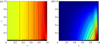
, are illustrated in figure 1. A thin Ekman layer is visible near
 $z=0$
, linked to the Ekman layer contributions
 $\widetilde{\unicode[STIX]{x1D713}}$
and
 $\widetilde{\unicode[STIX]{x1D714}}$
, identified by
 $\widetilde{{\unicode[STIX]{x1D713}\unicode[STIX]{x0030A}}}$
and
 $\widetilde{{\unicode[STIX]{x1D714}\unicode[STIX]{x0030A}}}$
as
 $\unicode[STIX]{x1D70F}\rightarrow \infty$
. The QG nature of the mainstream is demonstrated by the
 $\unicode[STIX]{x1D714}_{DNS}$
contours, which are almost parallel to the
 $z$
-axis in figure 1(a). The mainstream outflow caused by Ekman blowing is revealed by the tilted
 $\unicode[STIX]{x1D713}_{DNS}$
contours in figure 1(b), whose nature is consistent with the mainstream asymptotic result
 $$\begin{eqnarray}\unicode[STIX]{x1D713}=(z-1)\overline{\unicode[STIX]{x1D713}}(r)\approx -{\textstyle \frac{1}{2}}\unicode[STIX]{x1D70E}(z-1)r^{2}\overline{\unicode[STIX]{x1D714}}(r)\end{eqnarray}$$
determined by (2.11b
) and (2.28). This outflow is returned inside the
 $E^{1/3}$
sidewall layer (see § 4), evident near
 $r=\ell (=1)$
, to a sink, namely the
 $E^{1/2}\times E^{1/2}$
corner region in the neighbourhood of
 $(r,z)=(\ell ,0)$
. In turn, that influx is ejected within the
 $E^{1/2}$
Ekman layer at the base of the
 $E^{1/3}$
layer to provide the Ekman layer flux needed to adjust the QG flow.
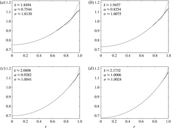
Comparison of ENS results
 $\overline{\unicode[STIX]{x1D714}}_{ENS}(r)$
(see (2.32); continuous dark line) and
 $\unicode[STIX]{x1D714}_{ENS}(r,1)$
(continuous light line), normalised by
 $\overline{\unicode[STIX]{x1D714}}_{ENS}(0)=\overline{\unicode[STIX]{x1D714}}(0)$
, with the entire analytic mainstream solution
 $\overline{\unicode[STIX]{x1D714}}(r)$
(dashed line) on
 $0\leqslant r\leqslant \ell (=1)$
. The plots are for the cases (a)
 $E=3\times 10^{-4}$
, (b)
 $E=10^{-4}$
, (c)
 $E=3\times 10^{-5}$
and (d)
 $E=10^{-5}$
. The values of
 $k$
,
 $\unicode[STIX]{x1D6FC}$
and
 $\unicode[STIX]{x1D70E}$
for each case are given on the respective plots.

2.4 Numerical eigensolution (ENS) for the case
$\ell =1$
for various
$E$


The DNS of the eigenvalue problem for (2.29), corresponding to the eigenvalue with largest real part, was achieved through time integration. The system was time-stepped, until a steadily decaying mode was obtained, without detailed consideration of the transient evolution. By that expedient, we were able to solve the eigenvalue problem for
 $\unicode[STIX]{x1D713}$
,
 $\unicode[STIX]{x1D714}$
(but only up to an arbitrary constant) and
 $q$
(i.e.,
 $\unicode[STIX]{x1D713}_{DNS}$
,
 $\unicode[STIX]{x1D714}_{DNS}$
and
 $q_{DNS}$
in (2.29)) for the case
 $\ell =1$
for various values of
 $E$
. We refer to it as the eigen (numerical) solution (ENS), for which
 $[\unicode[STIX]{x1D713},\unicode[STIX]{x1D714}]=[\unicode[STIX]{x1D713}_{ENS},\unicode[STIX]{x1D714}_{ENS}](r,z)$
and
 $q=q_{ENS}$
generate
 $\boldsymbol{u}_{ENS}$
. To place the results in context, we note that our asymptotic theory predicts
 $$\begin{eqnarray}\langle \breve{\unicode[STIX]{x1D714}}\rangle (r,t)\approx \unicode[STIX]{x1D707}\overline{\breve{\unicode[STIX]{x1D714}}}(r,t)\approx (\unicode[STIX]{x1D707}\unicode[STIX]{x1D705})\overline{\unicode[STIX]{x1D714}}(r)\exp (-q\ell ^{2}\unicode[STIX]{x1D70F})\quad \text{as }\unicode[STIX]{x1D70F}\rightarrow \infty\end{eqnarray}$$
(see (2.7), (2.20), (2.21) and (2.29)), where
 $\overline{\unicode[STIX]{x1D714}}(r)$
is defined by (2.23). Since the notion of a mainstream QG flow and an Ekman layer is an asymptotic (
 $E\ll 1$
) concept,
 $\overline{\unicode[STIX]{x1D714}}_{ENS}(r)$
evaluated at finite
 $E$
is not clearly defined. To overcome this obstacle, we simply set
 $$\begin{eqnarray}\overline{\unicode[STIX]{x1D714}}_{ENS}(r)\equiv \unicode[STIX]{x1D707}^{-1}\langle \unicode[STIX]{x1D714}_{ENS}\rangle (r)\end{eqnarray}$$
so that comparisons can be made with asymptotic theory for which
 $q$
in (2.31) is unfortunately as yet unknown. However, on assuming that
 $q=q_{ENS}$
, we may infer that the value of
 $k$
characterising our analytic solution
 $\overline{\unicode[STIX]{x1D714}}(r)$
(see (2.23)) is given by
 $k^{2}=\ell ^{2}(\unicode[STIX]{x1D70E}E^{-1/2}-q_{ENS})$
(see (1.10b
)). As the amplitude of the eigenfunction
 $\unicode[STIX]{x1D714}_{ENS}(r,z)$
is arbitrary, we simply normalise it by
 $\overline{\unicode[STIX]{x1D714}}_{ENS}(0)=\overline{\unicode[STIX]{x1D714}}(0)$
. If the ENS is truly QG, we expect the upper boundary value
 $\unicode[STIX]{x1D714}_{ENS}(r,1)$
to equal
 $\overline{\unicode[STIX]{x1D714}}(r)$
. For that reason, we compare the plots of
 $\overline{\unicode[STIX]{x1D714}}(r)$
,
 $\overline{\unicode[STIX]{x1D714}}_{ENS}(r)$
and
 $\unicode[STIX]{x1D714}_{ENS}(r,1)$
in figure 2(a–d) for various values of
 $E$
. The plots confirm our mainstream expectations:
 $\overline{\unicode[STIX]{x1D714}}(r)\approx \overline{\unicode[STIX]{x1D714}}_{ENS}(r)\approx \unicode[STIX]{x1D714}_{ENS}(r,1)$
. Their values only differ significantly within the
 $E^{1/3}$
sidewall (
 $r=\ell$
) layer. The strength of that layer is indicated by the amplitude of the oscillations
 $\unicode[STIX]{x1D714}_{ENS}(r,1)-\overline{\unicode[STIX]{x1D714}}(r)=O(E^{1/6})$
. The magnitude of the oscillations
 $\overline{\unicode[STIX]{x1D714}}_{ENS}(r)-\overline{\unicode[STIX]{x1D714}}(r)=O(E^{1/3})$
is markedly smaller. The relative sizes are clearly visible on the plots, while the theory behind the orders of magnitude alluded to will be explained in § 4.
We emphasise that so far the decay rate
 $q$
has been predicted by the ENS. To obtain a closed-form analytic solution we need to determine the value of
 $\unicode[STIX]{x1D6FC}$
that characterises the mainstream boundary condition
 $\text{d}\overline{\unicode[STIX]{x1D714}}/\text{d}r(\ell )=\unicode[STIX]{x1D6FC}\overline{\unicode[STIX]{x1D714}}(\ell )$
(see (2.24c
)) by consideration of the
 $E^{1/3}$
sidewall layer. With
 $\unicode[STIX]{x1D6FC}$
known, the
 $\unicode[STIX]{x1D70F}$
growth rate
 $k^{2}$
(see (2.21)) is given by the solution
 $k=k({\unicode[STIX]{x1D6FC}\unicode[STIX]{x0030A}})$
of
 $(k/\ell )\text{I}_{2}(k)/\text{I}_{1}(k)={\unicode[STIX]{x1D6FC}\unicode[STIX]{x0030A}}=\ell \unicode[STIX]{x1D6FC}$
(see (2.24b,d
)). That strategy, attempted in § 4.1, is hindered by the asymptotic orderings
 $\unicode[STIX]{x1D714}(r,z)-\overline{\unicode[STIX]{x1D714}}(r)=O(E^{1/6})$
,
 $\unicode[STIX]{x1D707}^{-1}\langle \unicode[STIX]{x1D714}\rangle (r)-\overline{\unicode[STIX]{x1D714}}(r)=O(E^{1/3})$
hinted at by figure 2(a–d). In short, although we are able to solve the vital
 $O(E^{1/3})$
problem for the relatively small shear-layer correction
 $\unicode[STIX]{x1D707}^{-1}\langle \unicode[STIX]{x1D714}\rangle -\overline{\unicode[STIX]{x1D714}}$
, the tiny size of
 $E$
needed for its validity is unreachable by our ENS. To bypass this difficulty, in § 4.2 we consider the shear-layer problem numerically retaining the relevant terms involving
 $E$
needed to encompass both the
 $O(E^{1/6})$
and
 $O(E^{1/3})$
problems simultaneously. From this hybrid asymptotic–numerical method, we determine
 $\unicode[STIX]{x1D6FC}$
and in turn
 ${\unicode[STIX]{x1D6FC}\unicode[STIX]{x0030A}}=\ell \unicode[STIX]{x1D6FC}$
and
 $k=k({\unicode[STIX]{x1D6FC}\unicode[STIX]{x0030A}})$
for various values of
 $E$
. The ENS value
 $q_{ENS}$
and the hybrid asymptotic–numerical value
 $q=\unicode[STIX]{x1D70E}E^{-1/2}-k^{2}\ell ^{-2}$
agree so well that for the purpose of plotting the graphs in figures 2(a–d), they are essentially the same. The weak dependence of
 $k$
and
 $\unicode[STIX]{x1D6FC}$
on
 $E$
evident from their values itemised in each respective plot proves to be a delicate issue that we discuss in § 4, but particularly in § 4.1.
3 The transient evolution of the QG azimuthal angular velocity
We consider the evolution of
 $\overline{{\unicode[STIX]{x1D714}\unicode[STIX]{x0030A}}}(r,\unicode[STIX]{x1D70F})$
, which solves
 $$\begin{eqnarray}\frac{\unicode[STIX]{x2202}\overline{{\unicode[STIX]{x1D714}\unicode[STIX]{x0030A}}}}{\unicode[STIX]{x2202}\unicode[STIX]{x1D70F}}=\ell ^{2}\left(\frac{\unicode[STIX]{x2202}^{2}\overline{{\unicode[STIX]{x1D714}\unicode[STIX]{x0030A}}}}{\unicode[STIX]{x2202}r^{2}}+\frac{3}{r}\frac{\unicode[STIX]{x2202}\overline{{\unicode[STIX]{x1D714}\unicode[STIX]{x0030A}}}}{\unicode[STIX]{x2202}r}\right)={\displaystyle \frac{\ell ^{2}}{r^{3}}}\frac{\unicode[STIX]{x2202}\unicode[STIX]{x1D6E4}}{\unicode[STIX]{x2202}r},\quad \unicode[STIX]{x1D6E4}=r^{3}\frac{\unicode[STIX]{x2202}\overline{{\unicode[STIX]{x1D714}\unicode[STIX]{x0030A}}}}{\unicode[STIX]{x2202}r}\end{eqnarray}$$
(see (2.13)) on the
 $\unicode[STIX]{x1D70F}=O(1)$
time scale. Here,
 $\overline{{\unicode[STIX]{x1D714}\unicode[STIX]{x0030A}}}(r,\unicode[STIX]{x1D70F})$
defines the actual QG angular velocity
 $$\begin{eqnarray}\overline{\breve{\unicode[STIX]{x1D714}}}(r,t)=\unicode[STIX]{x1D705}\overline{{\unicode[STIX]{x1D714}\unicode[STIX]{x0030A}}}(r,\unicode[STIX]{x1D70F})\exp (-\unicode[STIX]{x1D70E}E^{1/2}t)\end{eqnarray}$$
(see (2.7a
)), while
 $\unicode[STIX]{x1D6E4}$
provides a measure of the total viscous couple on cylinders of fluid radius
 $r$
. We need to solve (3.1) subject to the (
 $\unicode[STIX]{x1D70F}=0$
) initial condition
 $$\begin{eqnarray}\overline{{\unicode[STIX]{x1D714}\unicode[STIX]{x0030A}}}=1\quad \text{on }0<r<\ell ,\end{eqnarray}$$
determined by the spin-down solution (1.3a ), and the boundary conditions
 $$\begin{eqnarray}{\displaystyle \frac{1}{\ell ^{2}}}\unicode[STIX]{x1D6E4}=\ell \frac{\unicode[STIX]{x2202}\overline{{\unicode[STIX]{x1D714}\unicode[STIX]{x0030A}}}}{\unicode[STIX]{x2202}r}=\left\{\begin{array}{@{}ll@{}}0\quad & \text{at }r=0,\\ {\unicode[STIX]{x1D6FC}\unicode[STIX]{x0030A}}\overline{{\unicode[STIX]{x1D714}\unicode[STIX]{x0030A}}}\quad & \text{at }r=\ell .\end{array}\right.\end{eqnarray}$$
With
 ${\unicode[STIX]{x1D6FC}\unicode[STIX]{x0030A}}=\ell \unicode[STIX]{x1D6FC}>0$
, the outer boundary condition
 $\unicode[STIX]{x1D6E4}(\ell ,\unicode[STIX]{x1D70F})=\ell ^{2}{\unicode[STIX]{x1D6FC}\unicode[STIX]{x0030A}}\overline{{\unicode[STIX]{x1D714}\unicode[STIX]{x0030A}}}(\ell ,\unicode[STIX]{x1D70F})$
(see (2.24a,b
)) says that azimuthal motion at the outer boundary leads to a couple that accelerates rather than brakes the total rotational angular momentum
 $r^{3}\overline{{\unicode[STIX]{x1D714}\unicode[STIX]{x0030A}}}$
on cylinder radius
 $r$
.
Park & Hyun (Reference Park and Hyun1997), in their discussion of compressible Stewartson layers, provided the complete transient solution of a diffusion equation similar to (3.1). For our purposes, it is sufficient to note that, as
 $\unicode[STIX]{x1D70F}\rightarrow \infty$
, the asymptotic solution is given by (2.21). It is simply the first term of a modal expansion
 $$\begin{eqnarray}\overline{{\unicode[STIX]{x1D714}\unicode[STIX]{x0030A}}}(r,\unicode[STIX]{x1D70F})=A_{0}\overline{{\unicode[STIX]{x1D714}\unicode[STIX]{x0030A}}}_{0}(r)\exp (k^{2}\unicode[STIX]{x1D70F})+\mathop{\sum }_{n=1}^{\infty }A_{n}\overline{{\unicode[STIX]{x1D714}\unicode[STIX]{x0030A}}}_{n}(r)\exp (-k_{n}^{2}\unicode[STIX]{x1D70F}),\end{eqnarray}$$
where
 $\overline{{\unicode[STIX]{x1D714}\unicode[STIX]{x0030A}}}_{0}(r)$
defined by (2.23) solves (2.22). The eigenfunctions
 $$\begin{eqnarray}\overline{{\unicode[STIX]{x1D714}\unicode[STIX]{x0030A}}}_{n}(r)=2(k_{n}r/\ell )^{-1}\text{J}_{1}(k_{n}r/\ell )\quad (n\geqslant 1)\end{eqnarray}$$
solve (2.22) with
 $k^{2}$
replaced by the eigenvalues
 $-k_{n}^{2}$
, which are determined by the boundary conditions (3.4):
 $$\begin{eqnarray}k_{n}\text{J}_{2}(k_{n})=-{\unicode[STIX]{x1D6FC}\unicode[STIX]{x0030A}}\text{J}_{1}(k_{n}).\end{eqnarray}$$
Since the eigenfunctions
 $\overline{{\unicode[STIX]{x1D714}\unicode[STIX]{x0030A}}}_{n}(r)$
are orthogonal,
 $$\begin{eqnarray}\int _{0}^{\ell }\overline{{\unicode[STIX]{x1D714}\unicode[STIX]{x0030A}}}_{n}\overline{{\unicode[STIX]{x1D714}\unicode[STIX]{x0030A}}}_{m}r^{3}\,\text{d}r=0\quad (m\not =n),\end{eqnarray}$$
the initial condition
 $\overline{{\unicode[STIX]{x1D714}\unicode[STIX]{x0030A}}}(r,0)=1$
determines
 $$\begin{eqnarray}\int _{0}^{\ell }\overline{{\unicode[STIX]{x1D714}\unicode[STIX]{x0030A}}}r^{3}\,\text{d}r=A_{0}\int _{0}^{\ell }\overline{{\unicode[STIX]{x1D714}\unicode[STIX]{x0030A}}}^{2}r^{3}\,\text{d}r,\end{eqnarray}$$
which on substitution of
 $\overline{{\unicode[STIX]{x1D714}\unicode[STIX]{x0030A}}}_{0}(r)=2(kr/\ell )^{-1}\text{I}_{1}(kr/\ell )$
(see (2.23)) gives (2.25).
The solution corresponding to (3.5) for the Greenspan & Howard (Reference Greenspan and Howard1963) problem with the rigid outer wall, at which
 $\overline{{\unicode[STIX]{x1D714}\unicode[STIX]{x0030A}}}(\ell ,\unicode[STIX]{x1D70F})=0$
, is
 $$\begin{eqnarray}\overline{{\unicode[STIX]{x1D714}\unicode[STIX]{x0030A}}}(r,\unicode[STIX]{x1D70F})=\mathop{\sum }_{n=1}^{\infty }2B_{n}(j_{n}r/\ell )^{-1}\text{J}_{1}(j_{n}r/\ell )\exp (-j_{n}^{2}\unicode[STIX]{x1D70F})\end{eqnarray}$$
(cf. Park & Hyun Reference Park and Hyun1997, equation (19)), where the
 $j_{n}({>}0)$
are the zeros of the Bessel function
 $\text{J}_{1}$
. The slowest decaying mode
 $n=1$
has
 $$\begin{eqnarray}j_{1}=3.8317\cdots \,,\end{eqnarray}$$
while its amplitude
 $B_{1}$
is determined in the same way as
 $A_{0}$
above and is given in (5.2). It should be noted also that the modal growth rates
 $-j_{n}^{2}$
alternate with ours:
 $$\begin{eqnarray}k^{2}({>}0)>-j_{1}^{2}>-k_{1}^{2}>-j_{2}^{2}>-k_{2}^{2}>\cdots \,.\end{eqnarray}$$
3.1 Numerical results for the case
$\ell =1$
,
$E=10^{-4}$


We solved the reduced initial value problem (3.1), (3.3) and (3.4) for
 $\overline{{\unicode[STIX]{x1D714}\unicode[STIX]{x0030A}}}(r,\unicode[STIX]{x1D70F})$
numerically. The discontinuous nature of the initial condition can be handled by the discrete scheme, because the solution is regular for
 $\unicode[STIX]{x1D70F}>0$
. The numerical results obtained in this way can be compared with the results with the
 $z$
average
 $\langle \breve{\unicode[STIX]{x1D714}}_{DNS}\rangle (r,\unicode[STIX]{x1D70F})$
obtained from the DNS solution
 $\breve{\unicode[STIX]{x1D714}}_{DNS}(r,z,t)$
of the entire problem (2.4)–(2.6) for
 $\breve{\unicode[STIX]{x1D714}}(r,z,t)$
. To make that comparison, we need to build on our analytic predictions. First, the analysis of appendix A indicates that the amplitude of
 $\breve{\unicode[STIX]{x1D714}}$
is modified by the factor
 $\unicode[STIX]{x1D705}$
(see (1.3a,b
), also (A 9a
)) on the spin-down time scale
 $t=O(E^{-1/2})$
, equivalently
 $\unicode[STIX]{x1D70F}=O(E^{1/2})$
. Accordingly, we account for the spin-down decay rate and that amplitude modification in our analytic representation of the QG mainstream angular velocity
 $\overline{\breve{\unicode[STIX]{x1D714}}}(r,t)$
in (3.2). Second, our asymptotic results predict
 $\overline{\breve{\unicode[STIX]{x1D714}}}=\unicode[STIX]{x1D707}^{-1}\langle \breve{\unicode[STIX]{x1D714}}\rangle$
(see (2.20a,b
), also (A 9b
)), and so we define the corresponding DNS value by
 $$\begin{eqnarray}\overline{\breve{\unicode[STIX]{x1D714}}}_{DNS}(r,t)\equiv \unicode[STIX]{x1D707}^{-1}\langle \breve{\unicode[STIX]{x1D714}}_{DNS}\rangle (r,t),\end{eqnarray}$$
as in (2.32). Third, in view of the definition
 ${\unicode[STIX]{x1D714}\unicode[STIX]{x0030A}}=\unicode[STIX]{x1D705}^{-1}\breve{\unicode[STIX]{x1D714}}\exp (\unicode[STIX]{x1D70E}E^{1/2}t)$
(see (2.7)), we also define
 $$\begin{eqnarray}\overline{{\unicode[STIX]{x1D714}\unicode[STIX]{x0030A}}}_{DNS}(r,\unicode[STIX]{x1D70F})\equiv (\unicode[STIX]{x1D707}\unicode[STIX]{x1D705})^{-1}\langle \breve{\unicode[STIX]{x1D714}}_{DNS}\rangle (r,t)\exp (\unicode[STIX]{x1D70E}E^{1/2}t)\quad \text{for }\unicode[STIX]{x1D70F}=O(1),\end{eqnarray}$$
where
 $$\begin{eqnarray}(\unicode[STIX]{x1D707}\unicode[STIX]{x1D705})^{-1}=1+{\textstyle \frac{1}{4}}E^{1/2}+O(E)\end{eqnarray}$$
(see (A 9a,b )).
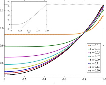
Profiles of
 $\overline{{\unicode[STIX]{x1D714}\unicode[STIX]{x0030A}}}_{DNS}(r,\unicode[STIX]{x1D70F})\exp (-k^{2}\unicode[STIX]{x1D70F})$
(continuous lines) for the case
 $E=10^{-4}$
,
 $\ell =1$
, for which
 $k\doteqdot 1.9457$
,
 ${\unicode[STIX]{x1D6FC}\unicode[STIX]{x0030A}}\doteqdot 0.8254$
,
 $\unicode[STIX]{x1D70E}\doteqdot 1.0075$
(see data on figure 2
b), at various times
 $\unicode[STIX]{x1D70F}$
, together with the corresponding profiles of
 $\overline{{\unicode[STIX]{x1D714}\unicode[STIX]{x0030A}}}(r,\unicode[STIX]{x1D70F})\exp (-k^{2}\unicode[STIX]{x1D70F})$
(dashed lines). The asymptotes
 $\overline{{\unicode[STIX]{x1D714}\unicode[STIX]{x0030A}}}(0,\unicode[STIX]{x1D70F})\exp (-k^{2}\unicode[STIX]{x1D70F})\downarrow A_{0}\doteqdot 0.7307$
and
 $\overline{{\unicode[STIX]{x1D714}\unicode[STIX]{x0030A}}}(\ell ,\unicode[STIX]{x1D70F})\exp (-k^{2}\unicode[STIX]{x1D70F})$
 $\uparrow A_{\ell }\doteqdot 1.1355$
as
 $\unicode[STIX]{x1D70F}\rightarrow \infty$
are indicated by the dotted lines. Inset: the left-hand end-point value
 $\log [\overline{{\unicode[STIX]{x1D714}\unicode[STIX]{x0030A}}}(0,\unicode[STIX]{x1D70F})]$
plotted versus
 $\unicode[STIX]{x1D70F}$
, together with its large-
 $\unicode[STIX]{x1D70F}$
asymptote
 $(\log A_{0})+k^{2}(\log \text{e})\unicode[STIX]{x1D70F}$
.

We illustrate the transient development of
 $\overline{{\unicode[STIX]{x1D714}\unicode[STIX]{x0030A}}}(r,\unicode[STIX]{x1D70F})$
and
 $\overline{{\unicode[STIX]{x1D714}\unicode[STIX]{x0030A}}}_{DNS}(r,\unicode[STIX]{x1D70F})$
for aspect ratio
 $\ell =1$
and
 $E=10^{-4}$
in figure 3, with other data itemised in the caption. Since (3.5) determines the late-time behaviour
 $$\begin{eqnarray}\overline{{\unicode[STIX]{x1D714}\unicode[STIX]{x0030A}}}(r,\unicode[STIX]{x1D70F})\approx A_{0}\overline{{\unicode[STIX]{x1D714}\unicode[STIX]{x0030A}}}_{0}(r)\exp (k^{2}\unicode[STIX]{x1D70F})\quad \text{as }\unicode[STIX]{x1D70F}\rightarrow \infty ,\end{eqnarray}$$
we remove this exponential growth and plot
 $\overline{{\unicode[STIX]{x1D714}\unicode[STIX]{x0030A}}}(r,\unicode[STIX]{x1D70F})\exp (-k^{2}\unicode[STIX]{x1D70F})$
and
 $\overline{{\unicode[STIX]{x1D714}\unicode[STIX]{x0030A}}}_{DNS}(r,\unicode[STIX]{x1D70F})\exp (-k^{2}\unicode[STIX]{x1D70F})$
instead at various times
 $\unicode[STIX]{x1D70F}$
. The
 $O(E^{1/2})$
correction to
 $\overline{{\unicode[STIX]{x1D714}\unicode[STIX]{x0030A}}}_{DNS}$
(see (3.10a
)) that ensues through the factor
 $(\unicode[STIX]{x1D707}\unicode[STIX]{x1D705})^{-1}$
(see (3.10b
)) leads to very good agreement between the respective curves at each
 $\unicode[STIX]{x1D70F}$
. Indeed, they are largely indistinguishable except in the
 $E^{1/3}$
sidewall layer, where
 $\overline{{\unicode[STIX]{x1D714}\unicode[STIX]{x0030A}}}_{DNS}$
needs to adjust to meet the boundary condition
 $\unicode[STIX]{x2202}\overline{{\unicode[STIX]{x1D714}\unicode[STIX]{x0030A}}}_{DNS}/\unicode[STIX]{x2202}r=0$
at
 $r=\ell (=1)$
. Similar discrepancies are visible in figure 2(b).
As noted in the early-time asymptotics of the following § 3.2, the left-hand (or centre) value
 $\overline{{\unicode[STIX]{x1D714}\unicode[STIX]{x0030A}}}(0,\unicode[STIX]{x1D70F})$
remains at unity until it eventually increases in response to diffusion across the domain driven by the right-hand (or outer) boundary condition. Eventually,
 $\overline{{\unicode[STIX]{x1D714}\unicode[STIX]{x0030A}}}(0,\unicode[STIX]{x1D70F})$
grows exponentially (see (3.11)). To illustrate this behaviour, we plot
 $\log [\overline{{\unicode[STIX]{x1D714}\unicode[STIX]{x0030A}}}(0,\unicode[STIX]{x1D70F})]$
versus
 $\unicode[STIX]{x1D70F}$
together with its large-
 $\unicode[STIX]{x1D70F}$
asymptote (it should be recalled that
 $\overline{{\unicode[STIX]{x1D714}\unicode[STIX]{x0030A}}}_{0}(0)=1$
) in the inset to figure 3. It suggests a transition between small- and large-
 $\unicode[STIX]{x1D70F}$
behaviour over roughly the range
 $0.05\lessapprox \unicode[STIX]{x1D70F}\lessapprox 0.1$
. This view is supported by figure 3 itself, in which
 $\overline{{\unicode[STIX]{x1D714}\unicode[STIX]{x0030A}}}(r,\unicode[STIX]{x1D70F})\exp (-k^{2}\unicode[STIX]{x1D70F})$
begins with the value unity at
 $\unicode[STIX]{x1D70F}=0$
. As time proceeds, the flatness of the profiles near
 $r=0$
for
 $\unicode[STIX]{x1D70F}=0.01$
and
 $0.03$
has largely disappeared by
 $\unicode[STIX]{x1D70F}=0.11$
. Subsequently, the left (
 $r=0$
) and right (
 $r=\ell$
) end-point values decrease and increase (respectively), monotonically approaching the respective values
 $A_{0}$
and
 $A_{\ell }$
(see (2.27)) as
 $\unicode[STIX]{x1D70F}\rightarrow \infty$
.
3.2 A short-time (
$\unicode[STIX]{x1D70F}\ll 1$
) series expansion

The initial condition
 $\overline{{\unicode[STIX]{x1D714}\unicode[STIX]{x0030A}}}=1$
(see (3.3)) satisfies the governing equation (3.1) and the boundary condition (3.4) at
 $r=0$
but not at
 $r=\ell$
. The discontinuity at
 $r=\ell$
is readily accommodated by the similarity solution
 $$\begin{eqnarray}\ell \frac{\unicode[STIX]{x2202}\overline{{\unicode[STIX]{x1D714}\unicode[STIX]{x0030A}}}}{\unicode[STIX]{x2202}r}={\unicode[STIX]{x1D6FC}\unicode[STIX]{x0030A}}\operatorname{erfc}\unicode[STIX]{x1D701},\quad \text{where }\unicode[STIX]{x1D701}={\displaystyle \frac{1-(r/\ell )}{\sqrt{4\unicode[STIX]{x1D70F}}}},\end{eqnarray}$$
which solves
 $\unicode[STIX]{x2202}\overline{{\unicode[STIX]{x1D714}\unicode[STIX]{x0030A}}}/\unicode[STIX]{x2202}\unicode[STIX]{x1D70F}=\ell ^{2}\unicode[STIX]{x2202}^{2}\overline{{\unicode[STIX]{x1D714}\unicode[STIX]{x0030A}}}/\unicode[STIX]{x2202}r^{2}$
and meets the initial condition
 $\unicode[STIX]{x2202}\overline{{\unicode[STIX]{x1D714}\unicode[STIX]{x0030A}}}/\unicode[STIX]{x2202}r(r,0)=0$
and the boundary conditions
 $\ell \unicode[STIX]{x2202}\overline{{\unicode[STIX]{x1D714}\unicode[STIX]{x0030A}}}/\unicode[STIX]{x2202}r(\ell ,\unicode[STIX]{x1D70F})={\unicode[STIX]{x1D6FC}\unicode[STIX]{x0030A}}$
and
 $\ell \unicode[STIX]{x2202}\overline{{\unicode[STIX]{x1D714}\unicode[STIX]{x0030A}}}/\unicode[STIX]{x2202}r\rightarrow 0$
as
 $\unicode[STIX]{x1D701}\rightarrow \infty$
. Integration with respect to
 $r$
yields
 $$\begin{eqnarray}\overline{{\unicode[STIX]{x1D714}\unicode[STIX]{x0030A}}}=1+{\unicode[STIX]{x1D6FC}\unicode[STIX]{x0030A}}\sqrt{4\unicode[STIX]{x1D70F}}\unicode[STIX]{x1D71B}_{1}(\unicode[STIX]{x1D701}),\quad \text{with }\unicode[STIX]{x1D71B}_{1}^{\prime }(\unicode[STIX]{x1D701})=-\operatorname{erfc}\unicode[STIX]{x1D701},\end{eqnarray}$$
giving
 $$\begin{eqnarray}\unicode[STIX]{x1D71B}_{1}(\unicode[STIX]{x1D701})=\int _{\unicode[STIX]{x1D701}}^{\infty }\operatorname{erfc}\unicode[STIX]{x1D701}\,\text{d}\unicode[STIX]{x1D701}={\displaystyle \frac{1}{\sqrt{\unicode[STIX]{x03C0}}}}\exp (-\unicode[STIX]{x1D701}^{2})-\unicode[STIX]{x1D701}\operatorname{erfc}\unicode[STIX]{x1D701}.\end{eqnarray}$$
The similarity solution (3.13) is the first term of an asymptotic power series solution
 $$\begin{eqnarray}\overline{{\unicode[STIX]{x1D714}\unicode[STIX]{x0030A}}}=1+{\unicode[STIX]{x1D6FC}\unicode[STIX]{x0030A}}\mathop{\sum }_{n=1}^{\infty }(4\unicode[STIX]{x1D70F})^{n/2}\unicode[STIX]{x1D71B}_{n}(\unicode[STIX]{x1D701}),\quad \text{valid on }0<\unicode[STIX]{x1D701}<(4\unicode[STIX]{x1D70F})^{-1/2},\end{eqnarray}$$
for
 $\unicode[STIX]{x1D70F}\ll 1$
. We outline the solution built around (B 4)–(B 5) in appendix B.
As a diagnostic for comparison with our direct numerical solution of (3.1)–(3.4), we note that the end-point value (B 7) at
 $r=\ell$
determined by the terms (B 6) and (B 8)–(B 11), up to
 $n=4$
, is
 $$\begin{eqnarray}\displaystyle \overline{{\unicode[STIX]{x1D714}\unicode[STIX]{x0030A}}}(\ell ,\unicode[STIX]{x1D70F}) & {\approx} & \displaystyle 1+{\displaystyle \frac{2{\unicode[STIX]{x1D6FC}\unicode[STIX]{x0030A}}}{\sqrt{\unicode[STIX]{x03C0}}}}\unicode[STIX]{x1D70F}^{1/2}+{\unicode[STIX]{x1D6FC}\unicode[STIX]{x0030A}}\left({\displaystyle \frac{3}{2}}+{\unicode[STIX]{x1D6FC}\unicode[STIX]{x0030A}}\right)\unicode[STIX]{x1D70F}+{\displaystyle \frac{{\unicode[STIX]{x1D6FC}\unicode[STIX]{x0030A}}}{\sqrt{\unicode[STIX]{x03C0}}}}\left({\displaystyle \frac{5}{2}}+4{\unicode[STIX]{x1D6FC}\unicode[STIX]{x0030A}}+{\displaystyle \frac{4}{3}}{\unicode[STIX]{x1D6FC}\unicode[STIX]{x0030A}}^{2}\right)\unicode[STIX]{x1D70F}^{3/2}\nonumber\\ \displaystyle & & \displaystyle +\,{\displaystyle \frac{3{\unicode[STIX]{x1D6FC}\unicode[STIX]{x0030A}}}{4}}\left({\displaystyle \frac{5}{4}}+4{\unicode[STIX]{x1D6FC}\unicode[STIX]{x0030A}}+3{\unicode[STIX]{x1D6FC}\unicode[STIX]{x0030A}}^{2}+{\displaystyle \frac{2}{3}}{\unicode[STIX]{x1D6FC}\unicode[STIX]{x0030A}}^{3}\right)\unicode[STIX]{x1D70F}^{2}+O(\unicode[STIX]{x1D70F}^{5/2}).\end{eqnarray}$$
To compare with the large-
 $\unicode[STIX]{x1D70F}$
solution
 $\overline{{\unicode[STIX]{x1D714}\unicode[STIX]{x0030A}}}(r,\unicode[STIX]{x1D70F})=\overline{\unicode[STIX]{x1D714}}(r)\exp (k^{2}\unicode[STIX]{x1D70F})$
, we expand
 $\overline{{\unicode[STIX]{x1D714}\unicode[STIX]{x0030A}}}(r,\unicode[STIX]{x1D70F})\exp (-k^{2}\unicode[STIX]{x1D70F})$
at both
 $r=0$
and
 $r=\ell$
to the same order of accuracy:
 $$\begin{eqnarray}\displaystyle \overline{{\unicode[STIX]{x1D714}\unicode[STIX]{x0030A}}}(0,\unicode[STIX]{x1D70F})\exp (-k^{2}\unicode[STIX]{x1D70F}) & {\approx} & \displaystyle \exp (-k^{2}\unicode[STIX]{x1D70F})\approx 1-k^{2}\unicode[STIX]{x1D70F}+{\textstyle \frac{1}{2}}k^{4}\unicode[STIX]{x1D70F}^{2}+O(\unicode[STIX]{x1D70F}^{3}),\end{eqnarray}$$
 $$\begin{eqnarray}\displaystyle \overline{{\unicode[STIX]{x1D714}\unicode[STIX]{x0030A}}}(\ell ,\unicode[STIX]{x1D70F})\exp (-k^{2}\unicode[STIX]{x1D70F}) & {\approx} & \displaystyle 1+{\displaystyle \frac{2{\unicode[STIX]{x1D6FC}\unicode[STIX]{x0030A}}}{\sqrt{\unicode[STIX]{x03C0}}}}\unicode[STIX]{x1D70F}^{1/2}+\left[{\unicode[STIX]{x1D6FC}\unicode[STIX]{x0030A}}\left({\displaystyle \frac{3}{2}}+{\unicode[STIX]{x1D6FC}\unicode[STIX]{x0030A}}\right)-k^{2}\right]\unicode[STIX]{x1D70F}\nonumber\\ \displaystyle & & \displaystyle +\,{\displaystyle \frac{{\unicode[STIX]{x1D6FC}\unicode[STIX]{x0030A}}}{\sqrt{\unicode[STIX]{x03C0}}}}\left({\displaystyle \frac{5}{2}}+4{\unicode[STIX]{x1D6FC}\unicode[STIX]{x0030A}}+{\displaystyle \frac{4}{3}}{\unicode[STIX]{x1D6FC}\unicode[STIX]{x0030A}}^{2}-2k^{2}\right)\unicode[STIX]{x1D70F}^{3/2}\nonumber\\ \displaystyle & & \displaystyle +\,\left[{\displaystyle \frac{3{\unicode[STIX]{x1D6FC}\unicode[STIX]{x0030A}}}{4}}\left({\displaystyle \frac{5}{4}}+4{\unicode[STIX]{x1D6FC}\unicode[STIX]{x0030A}}+3{\unicode[STIX]{x1D6FC}\unicode[STIX]{x0030A}}^{2}+{\displaystyle \frac{2}{3}}{\unicode[STIX]{x1D6FC}\unicode[STIX]{x0030A}}^{3}\right)-k^{2}{\unicode[STIX]{x1D6FC}\unicode[STIX]{x0030A}}\left({\displaystyle \frac{3}{2}}+{\unicode[STIX]{x1D6FC}\unicode[STIX]{x0030A}}\right)+{\displaystyle \frac{1}{2}}k^{4}\right]\unicode[STIX]{x1D70F}^{2}\nonumber\\ \displaystyle & & \displaystyle +\,O(\unicode[STIX]{x1D70F}^{5/2}).\end{eqnarray}$$
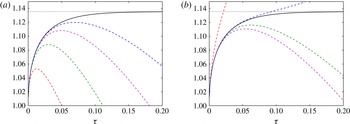
Returning to results from the direct numerical solution of (3.1)–(3.4), whereas in the inset of figure 3 we plot the logarithm of the left-hand end-point value
 $\overline{{\unicode[STIX]{x1D714}\unicode[STIX]{x0030A}}}(0,\unicode[STIX]{x1D70F})$
, in figure 4(a) we plot the right-hand end-point value
 $\overline{{\unicode[STIX]{x1D714}\unicode[STIX]{x0030A}}}(\ell ,\unicode[STIX]{x1D70F})\exp (-k^{2}\unicode[STIX]{x1D70F})$
. We also show the approximations derived by using the power series representation of
 $\overline{{\unicode[STIX]{x1D714}\unicode[STIX]{x0030A}}}(\ell ,\unicode[STIX]{x1D70F})$
given by the series expansion (3.15) truncated at various levels. The first
 $n=1$
term truncation (3.13a,b
) identifies the
 $\unicode[STIX]{x1D70F}^{1/2}$
singular behaviour near
 $\unicode[STIX]{x1D70F}=0$
but only gives a good approximation for very small
 $\unicode[STIX]{x1D70F}$
. Further terms improve the
 $\unicode[STIX]{x1D70F}$
range of usefulness considerably. In figure 4(b), we employ the complete power series representation (3.16b
) of
 $\overline{{\unicode[STIX]{x1D714}\unicode[STIX]{x0030A}}}(\ell ,\unicode[STIX]{x1D70F})\exp (-k^{2}\unicode[STIX]{x1D70F})$
, which interestingly for even
 $n$
(i.e.
 $n=2$
,
 $4$
) improves the approximation, exhibiting a longer
 $\unicode[STIX]{x1D70F}$
range of usefulness at each level of truncation. The improvement is not apparent for odd
 $n$
(i.e.
 $n=1$
,
 $3$
). It is worth noting that the best (
 $n=4$
) truncation provides a reasonable approximation until
 $\unicode[STIX]{x1D70F}\sim 0.1$
, by which time the solution portrayed in figure 3 is close to its final asymptotic
 $\unicode[STIX]{x1D70F}\rightarrow \infty$
form. It must be appreciated that the power series solution (B 7) described in appendix B is truly asymptotic, not least because it takes no account of the left-hand (
 $r=0$
) boundary condition.
The right-hand end-point value
 $\overline{{\unicode[STIX]{x1D714}\unicode[STIX]{x0030A}}}(\ell ,\unicode[STIX]{x1D70F})\exp (-k^{2}\unicode[STIX]{x1D70F})$
(solid line) plotted versus
 $\unicode[STIX]{x1D70F}$
for the case illustrated in figure 3. (a) The dashed curves correspond to
 $\overline{{\unicode[STIX]{x1D714}\unicode[STIX]{x0030A}}}(\ell ,\unicode[STIX]{x1D70F})$
given by the series expansion (3.15) truncated at various orders:
 $n=1$
, red;
 $2$
, green;
 $3$
, magenta;
 $4$
, blue (see (3.14)). (b) As in (a) but the power series for
 $\exp (-k^{2}\unicode[STIX]{x1D70F})$
is employed and the product (3.16b
) is again approximated at the various orders. We also show the asymptote
 $\overline{{\unicode[STIX]{x1D714}\unicode[STIX]{x0030A}}}(\ell ,\unicode[STIX]{x1D70F})\exp (-k^{2}\unicode[STIX]{x1D70F})$
 $\uparrow A_{\ell }\doteqdot 1.1355$
as
 $\unicode[STIX]{x1D70F}\rightarrow \infty$
(dotted line).

4 The
$E^{1/3}$
sidewall shear layer

We pointed out in § 1.1 that the
 $E^{1/3}$
shear layer adjacent to the outer cylinder wall
 $r=\ell$
is established on a time scale
 $t\sim E^{-1/3}$
short compared with the spin-up time
 $t\sim E^{-1/2}$
. Once established, its longer time evolution is best investigated via the modulation amplitudes
 ${\unicode[STIX]{x1D714}\unicode[STIX]{x0030A}}(r,z,\unicode[STIX]{x1D70F})$
and
 ${\unicode[STIX]{x1D713}\unicode[STIX]{x0030A}}(r,z,\unicode[STIX]{x1D70F})$
of the spin-down solution, which satisfy the scaled governing equations (2.9a,b
). Our ultimate objective is to establish analytically the value of
 $\unicode[STIX]{x1D6FC}$
in (2.24c
), which determines the mainstream boundary condition
 $\text{d}\overline{\unicode[STIX]{x1D714}}/\text{d}r=\unicode[STIX]{x1D6FC}\overline{\unicode[STIX]{x1D714}}$
at
 $r=\ell$
. This relation is only meaningful for
 $t\gg E^{-1/3}$
, by which time
 $\unicode[STIX]{x1D6FC}$
is well defined and independent of
 $t$
. Therefore, to determine
 $\unicode[STIX]{x1D6FC}$
it is sufficient to consider the final time eigenfunction
 $$\begin{eqnarray}\unicode[STIX]{x1D705}^{-1}[\breve{\unicode[STIX]{x1D713}},\breve{\unicode[STIX]{x1D714}}]\exp (q\ell ^{2}\unicode[STIX]{x1D70F})=[\unicode[STIX]{x1D713},\unicode[STIX]{x1D714}](r,z)\end{eqnarray}$$
(cf. (1.10a,b
) or equivalently (2.7a,b
) and (2.21)). Although formulated in this restricted sense for clarity, our shear-layer analysis pertains to all
 $t\gg E^{-1/3}$
upon making the approximation
 $q\ell ^{2}\unicode[STIX]{x1D70F}=E^{1/2}t$
in (4.1).
We restrict attention to the shear-layer flow outside the Ekman layer, and represent it as the sum of the QG mainstream solution (2.11a,b ) and a shear-layer correction:
 $$\begin{eqnarray}\unicode[STIX]{x1D714}=\overline{\unicode[STIX]{x1D714}}(r)+\unicode[STIX]{x1D700}\overline{\unicode[STIX]{x1D714}}(\ell )V(\unicode[STIX]{x1D701},z),\quad \unicode[STIX]{x1D713}=\overline{\unicode[STIX]{x1D713}}(r)(z-1)+\ell ^{2}\overline{\unicode[STIX]{x1D714}}(\ell )\unicode[STIX]{x1D6F9}(\unicode[STIX]{x1D701},z),\end{eqnarray}$$
where
 $$\begin{eqnarray}\overline{\unicode[STIX]{x1D713}}(r)=-{\textstyle \frac{1}{2}}\unicode[STIX]{x1D70E}r^{2}\overline{\unicode[STIX]{x1D714}}(r),\quad \unicode[STIX]{x1D701}=\unicode[STIX]{x1D700}^{-2}(r-\ell )\quad \text{and}\quad \unicode[STIX]{x1D700}=E^{1/6}\end{eqnarray}$$
(see (2.23) and (2.28), and also (2.30)). Here,
 $\unicode[STIX]{x1D701}$
is the stretched radial boundary layer coordinate and
 $\unicode[STIX]{x1D700}$
is the natural expansion parameter,
 $E^{1/3}=\unicode[STIX]{x1D700}^{2}$
and
 $E^{1/2}=\unicode[STIX]{x1D700}^{3}$
. The boundary layer corrections
 $V$
,
 $\unicode[STIX]{x1D6F9}$
must tend to zero as
 $\unicode[STIX]{x1D701}\rightarrow -\infty$
as well to ensure that the boundary conditions (2.6a
) at
 $r=\ell$
are met.
To extract the boundary layer equations correct to
 $O(\unicode[STIX]{x1D700})$
, it is sufficient to consider (2.9a,b
) with
 $\unicode[STIX]{x1D70E}\approx 1$
(so, e.g., (4.2c
) becomes
 $\overline{\unicode[STIX]{x1D713}}(r)=-(1/2)r^{2}\overline{\unicode[STIX]{x1D714}}(r)$
). They determine
 $$\begin{eqnarray}-2\frac{\unicode[STIX]{x2202}\unicode[STIX]{x1D6F9}}{\unicode[STIX]{x2202}z}=\frac{\unicode[STIX]{x2202}^{2}V}{\unicode[STIX]{x2202}\unicode[STIX]{x1D701}^{2}}+\unicode[STIX]{x1D700}V,\quad 2\frac{\unicode[STIX]{x2202}V}{\unicode[STIX]{x2202}z}=\frac{\unicode[STIX]{x2202}^{2}}{\unicode[STIX]{x2202}\unicode[STIX]{x1D701}^{2}}\left(\frac{\unicode[STIX]{x2202}^{2}\unicode[STIX]{x1D6F9}}{\unicode[STIX]{x2202}\unicode[STIX]{x1D701}^{2}}+\unicode[STIX]{x1D700}\unicode[STIX]{x1D6F9}\right).\end{eqnarray}$$
To the same order of accuracy, the boundary conditions (2.6a ) are
 $$\begin{eqnarray}\unicode[STIX]{x1D6F9}=\frac{1}{2}(z-1),\quad \frac{\unicode[STIX]{x2202}^{2}\unicode[STIX]{x1D6F9}}{\unicode[STIX]{x2202}\unicode[STIX]{x1D701}^{2}}=0,\quad \frac{\unicode[STIX]{x2202}V}{\unicode[STIX]{x2202}\unicode[STIX]{x1D701}}=-\unicode[STIX]{x1D700}\unicode[STIX]{x1D6FC}\quad \text{at }\unicode[STIX]{x1D701}=0,\end{eqnarray}$$
 $$\begin{eqnarray}\displaystyle \hspace{-16.99998pt}\phantom{\unicode[STIX]{x1D6F9}=\frac{1}{2}(z-1),\quad \frac{\unicode[STIX]{x2202}^{2}\unicode[STIX]{x1D6F9}}{\unicode[STIX]{x2202}\unicode[STIX]{x1D701}^{2}}=0,} & \phantom{\quad \displaystyle \frac{\unicode[STIX]{x2202}V}{\unicode[STIX]{x2202}\unicode[STIX]{x1D701}}=-\unicode[STIX]{x1D700}\unicode[STIX]{x1D6FC}} & \displaystyle \phantom{\text{at }\unicode[STIX]{x1D701}=0,}\nonumber\\ \displaystyle \hspace{-16.99998pt}\unicode[STIX]{x1D6F9}\rightarrow 0,\hspace{2.5pt} & \hspace{5.0pt}\quad V\rightarrow 0, & \displaystyle \hspace{0.2pt}\text{as }\unicode[STIX]{x1D701}\rightarrow -\infty ,\end{eqnarray}$$
for
 $0<z<1$
, where
 $\unicode[STIX]{x1D6FC}=\text{d}\overline{\unicode[STIX]{x1D714}}/\text{d}r(\ell )/\overline{\unicode[STIX]{x1D714}}(\ell )$
, while the Ekman jump condition at
 $z=0$
on the flow exterior to the Ekman layer and the symmetry conditions (2.6c
) at
 $z=1$
are respectively
 $$\begin{eqnarray}\unicode[STIX]{x1D6F9}={\textstyle \frac{1}{2}}\unicode[STIX]{x1D700}V\quad \hspace{45.50009pt}\text{at }z=0,\end{eqnarray}$$
 $$\begin{eqnarray}\unicode[STIX]{x1D6F9}=\frac{\unicode[STIX]{x2202}^{2}\unicode[STIX]{x1D6F9}}{\unicode[STIX]{x2202}z^{2}}=\frac{\unicode[STIX]{x2202}V}{\unicode[STIX]{x2202}z}=0\quad \text{at }z=1,\end{eqnarray}$$
for
 $\unicode[STIX]{x1D701}<0$
.
In view of the boundary conditions (4.4b ), we may introduce the new variable
 $$\begin{eqnarray}\unicode[STIX]{x1D6E9}(\unicode[STIX]{x1D701},z)=\int _{-\infty }^{\unicode[STIX]{x1D701}}V\,\text{d}\unicode[STIX]{x1D701}\quad \Longrightarrow \quad V=\frac{\unicode[STIX]{x2202}\unicode[STIX]{x1D6E9}}{\unicode[STIX]{x2202}\unicode[STIX]{x1D701}}\end{eqnarray}$$
and integrate (4.3b ). By this device, we may symmetrise the shear-layer equations (4.3a,b ) and express them in the compact complex form
 $$\begin{eqnarray}2\text{i}\frac{\unicode[STIX]{x2202}\unicode[STIX]{x1D6EF}}{\unicode[STIX]{x2202}z}=\frac{\unicode[STIX]{x2202}}{\unicode[STIX]{x2202}\unicode[STIX]{x1D701}}\left(\frac{\unicode[STIX]{x2202}^{2}\unicode[STIX]{x1D6EF}}{\unicode[STIX]{x2202}\unicode[STIX]{x1D701}^{2}}+\unicode[STIX]{x1D700}\unicode[STIX]{x1D6EF}\right),\end{eqnarray}$$
where
 $$\begin{eqnarray}\unicode[STIX]{x1D6EF}=\unicode[STIX]{x1D6E9}+\text{i}\unicode[STIX]{x1D6F9},\quad \text{giving}\quad \unicode[STIX]{x1D6F6}=V+\text{i}W=\frac{\unicode[STIX]{x2202}\unicode[STIX]{x1D6EF}}{\unicode[STIX]{x2202}\unicode[STIX]{x1D701}}\quad \left(W=\frac{\unicode[STIX]{x2202}\unicode[STIX]{x1D6F9}}{\unicode[STIX]{x2202}\unicode[STIX]{x1D701}}\right),\end{eqnarray}$$
which is also useful.
4.1 Asymptotic approach
We show in § 4.1.1 that, at zeroth order, the solution for
 $V(\unicode[STIX]{x1D701},z)$
has no
 $z$
mean, or, more precisely,
 $\langle V\rangle =O(\unicode[STIX]{x1D700})$
. The objective of the first-order problem investigated in § 4.1.3 is to solve (4.25) for
 $\langle V\rangle$
, which, in turn, determines our key quantity of interest,
 $\unicode[STIX]{x1D6FC}=-\unicode[STIX]{x1D700}^{-1}\,\text{d}\langle V\rangle /\text{d}\unicode[STIX]{x1D701}|_{\unicode[STIX]{x1D701}=0}$
, namely the
 $z$
average of (4.4a
)
 $_{3}$
.
4.1.1 The zeroth-order problem
On setting
 $\unicode[STIX]{x1D700}=0$
, the solution of (4.3)–(4.6) is
 $$\begin{eqnarray}\displaystyle \unicode[STIX]{x1D6EF}(\unicode[STIX]{x1D701},z) & = & \displaystyle -{\displaystyle \frac{2}{\sqrt{3}\unicode[STIX]{x03C0}}}\mathop{\sum }_{n=1}^{\infty }{\displaystyle \frac{(-1)^{n}}{n}}E(k_{n}\unicode[STIX]{x1D701};-\unicode[STIX]{x03C0}/6)\exp [\text{i}n\unicode[STIX]{x03C0}(z-1)],\end{eqnarray}$$
 $$\begin{eqnarray}\displaystyle \unicode[STIX]{x1D6F6}(\unicode[STIX]{x1D701},z) & = & \displaystyle -{\displaystyle \frac{2}{\sqrt{3}\unicode[STIX]{x03C0}}}\mathop{\sum }_{n=1}^{\infty }{\displaystyle \frac{(-1)^{n}k_{n}}{n}}E(k_{n}\unicode[STIX]{x1D701};\unicode[STIX]{x03C0}/6)\exp [\text{i}n\unicode[STIX]{x03C0}(z-1)],\end{eqnarray}$$
 $$\begin{eqnarray}k_{n}=(2n\unicode[STIX]{x03C0})^{1/3},\quad E(k_{n}\unicode[STIX]{x1D701};\unicode[STIX]{x1D6FC})=\exp ({\textstyle \frac{1}{2}}k_{n}\unicode[STIX]{x1D701})\cos [(\sqrt{3}/2)k_{n}\unicode[STIX]{x1D701}+\unicode[STIX]{x1D6FC}].\end{eqnarray}$$
Verification of the essential relation
 $\unicode[STIX]{x1D6F6}=\unicode[STIX]{x2202}\unicode[STIX]{x1D6EF}/\unicode[STIX]{x2202}\unicode[STIX]{x1D701}$
(see (4.6c
)) follows from the property
 $$\begin{eqnarray}\frac{\text{d}}{\text{d}\unicode[STIX]{x1D701}}E(k_{n}\unicode[STIX]{x1D701};\unicode[STIX]{x1D6FC})=k_{n}E(k_{n}\unicode[STIX]{x1D701};\unicode[STIX]{x1D6FC}+\unicode[STIX]{x03C0}/3)\quad \Longrightarrow \quad \frac{\text{d}^{3}E}{\text{d}\unicode[STIX]{x1D701}^{3}}=-k_{n}^{3}E\end{eqnarray}$$
also. Since
 $\text{Im}\{\exp [\text{i}n\unicode[STIX]{x03C0}(z-1)]\}=0$
at
 $z=0$
and
 $1$
, the boundary conditions (4.4c
), namely
 $\unicode[STIX]{x1D6F9}(\unicode[STIX]{x1D701},0)=0$
at the bottom and (4.4d
) at the top, are all obviously met. Another property of the solution on
 $z=0$
, useful later in § 4.1.3 (see (4.26b
)), is
 $$\begin{eqnarray}\int _{-\infty }^{\unicode[STIX]{x1D701}}\unicode[STIX]{x1D6E9}(\unicode[STIX]{x1D701},0)\,\text{d}\unicode[STIX]{x1D701}=\int _{-\infty }^{\unicode[STIX]{x1D701}}\unicode[STIX]{x1D6EF}(\unicode[STIX]{x1D701},0)\,\text{d}\unicode[STIX]{x1D701}=-{\displaystyle \frac{2}{\sqrt{3}\unicode[STIX]{x03C0}}}\mathop{\sum }_{n=1}^{\infty }{\displaystyle \frac{1}{nk_{n}}}E(k_{n}\unicode[STIX]{x1D701};-\unicode[STIX]{x03C0}/2),\end{eqnarray}$$
where we have used (4.8a ).
On use of (4.8b
), it is readily seen that
 $\unicode[STIX]{x1D6EF}$
, defined by (4.7a
), solves (4.6a
). Furthermore, since
 $$\begin{eqnarray}\frac{\text{d}^{2}}{\text{d}\unicode[STIX]{x1D701}^{2}}E(k_{n}\unicode[STIX]{x1D701};-\unicode[STIX]{x03C0}/6)|_{\unicode[STIX]{x1D701}=0}=k_{n}^{2}E(k_{n}\unicode[STIX]{x1D701};\unicode[STIX]{x03C0}/2)|_{\unicode[STIX]{x1D701}=0}=0,\end{eqnarray}$$
it is clear that the two boundary conditions
 $\unicode[STIX]{x2202}^{2}\unicode[STIX]{x1D6F9}/\unicode[STIX]{x2202}\unicode[STIX]{x1D701}^{2}=\unicode[STIX]{x2202}V/\unicode[STIX]{x2202}\unicode[STIX]{x1D701}=0$
at
 $\unicode[STIX]{x1D701}=0$
are met, i.e.
 $$\begin{eqnarray}\frac{\unicode[STIX]{x2202}^{2}\unicode[STIX]{x1D6EF}}{\unicode[STIX]{x2202}\unicode[STIX]{x1D701}^{2}}(0,z)=\frac{\unicode[STIX]{x2202}\unicode[STIX]{x1D6F6}}{\unicode[STIX]{x2202}\unicode[STIX]{x1D701}}(0,z)=0.\end{eqnarray}$$
Furthermore, (4.7a,b
) evaluated at
 $\unicode[STIX]{x1D701}=0$
determines
 $$\begin{eqnarray}\displaystyle \unicode[STIX]{x1D6EF}(0,z) & = & \displaystyle -{\displaystyle \frac{1}{\unicode[STIX]{x03C0}}}\mathop{\sum }_{n=1}^{\infty }{\displaystyle \frac{(-1)^{n}}{n}}\exp (\text{i}n\unicode[STIX]{x03C0}(z-1))={\displaystyle \frac{1}{\unicode[STIX]{x03C0}}}\ln [1+\exp (\text{i}\unicode[STIX]{x03C0}(z-1))]\nonumber\\ \displaystyle & = & \displaystyle \unicode[STIX]{x03C0}^{-1}\ln \left[2\sin \left(\frac{1}{2}\unicode[STIX]{x03C0}z\right)\right]+\frac{\text{i}}{2}(z-1)\end{eqnarray}$$
 $$\begin{eqnarray}\displaystyle & = & \displaystyle {\displaystyle \frac{1}{\unicode[STIX]{x03C0}}}\ln (\unicode[STIX]{x03C0}z)+{\displaystyle \frac{\text{i}}{2}}(-1+z)+\mathop{\sum }_{n=1}^{\infty }\unicode[STIX]{x1D6EF}_{n}z^{2n},\end{eqnarray}$$
 $$\begin{eqnarray}\displaystyle \frac{\unicode[STIX]{x2202}\unicode[STIX]{x1D6EF}}{\unicode[STIX]{x2202}\unicode[STIX]{x1D701}}(0,z) & = & \displaystyle \unicode[STIX]{x1D6F6}(0,z)=-{\displaystyle \frac{2^{1/3}}{\unicode[STIX]{x03C0}^{2/3}}}\mathop{\sum }_{n=1}^{\infty }{\displaystyle \frac{\exp (\text{i}n\unicode[STIX]{x03C0}z)}{n^{2/3}}}=-{\displaystyle \frac{2^{1/3}}{\unicode[STIX]{x03C0}^{2/3}}}\text{L}\text{i}_{2/3}(\text{e}^{\text{i}\unicode[STIX]{x03C0}z})\nonumber\\ \displaystyle & = & \displaystyle -{\displaystyle \frac{2^{1/3}\unicode[STIX]{x1D6E4}(1/3)\text{e}^{\text{i}\unicode[STIX]{x03C0}/6}}{\unicode[STIX]{x03C0}z^{1/3}}}+\mathop{\sum }_{n=0}^{\infty }\unicode[STIX]{x1D6F6}_{n}z^{n},\end{eqnarray}$$
 $\text{L}\text{i}_{2/3}(\unicode[STIX]{x1D702})=\sum _{n=1}^{\infty }n^{-2/3}z^{n}$
, and where
 $$\begin{eqnarray}\unicode[STIX]{x1D6EF}_{n}=-{\displaystyle \frac{\unicode[STIX]{x1D701}(2n)}{2^{2n}n\unicode[STIX]{x03C0}}},\quad \unicode[STIX]{x1D6F6}_{n}=-{\displaystyle \frac{2^{1/3}}{\unicode[STIX]{x03C0}^{2/3}}}\unicode[STIX]{x1D701}((2/3)-n){\displaystyle \frac{(\text{i}\unicode[STIX]{x03C0})^{n}}{n!}},\end{eqnarray}$$
in which
 $\unicode[STIX]{x1D701}(m)$
(
 $=\sum _{n=1}^{\infty }n^{-m}$
, for
 $m>1$
, and by analytic continuation elsewhere) is the Riemann Zeta function. The result (4.12a
) verifies that the boundary condition
 $\unicode[STIX]{x1D6F9}(0,z)=(z-1)/2$
is met, while in addition determining the result
 $\unicode[STIX]{x1D6E9}(0,z)=\unicode[STIX]{x03C0}^{-1}\ln [2\sin (\unicode[STIX]{x03C0}z/2)]$
. The series representations (4.12b,c
) follow on use of (http://dlmf.nist.gov/25.8.E8) and (http://dlmf.nist.gov/25.12.E12) respectively (here and below, we use this style of online reference to equations in Abramowitz & Stegun Reference Abramowitz, Stegun, Olver, Lozier, Boisvert and Clark2010) and are valid over the entire range
 $0<z\leqslant 1$
.
4.1.2 The power series solution
The power series forms (4.12b,c
) of the solution at
 $\unicode[STIX]{x1D701}=0$
identify clearly a singularity at
 $(\unicode[STIX]{x1D701},z)=(0,0)$
. To resolve it, we reconstruct the full solution (4.7a,b
) by solving the shear-layer equation (4.6a
) subject to the boundary conditions (4.11) and (4.12b,c
) at
 $\unicode[STIX]{x1D701}=0$
. These suggest the expansion
 $$\begin{eqnarray}\displaystyle \unicode[STIX]{x1D6EF}(\unicode[STIX]{x1D701},z) & = & \displaystyle \left[{\displaystyle \frac{1}{\unicode[STIX]{x03C0}}}\ln (\unicode[STIX]{x03C0}z)-{\displaystyle \frac{\text{i}}{2}}+\mathsf{Y}(\unicode[STIX]{x1D6F7})\right]+z\left[{\displaystyle \frac{\text{i}}{2}}-{\displaystyle \frac{1}{6}}\unicode[STIX]{x1D6F7}^{3}\right]+\widehat{\unicode[STIX]{x1D6EF}}(\unicode[STIX]{x1D6F7},z),\end{eqnarray}$$
 $$\begin{eqnarray}\displaystyle \unicode[STIX]{x1D6F6}(\unicode[STIX]{x1D701},z) & = & \displaystyle z^{-1/3}\mathsf{Z}(\unicode[STIX]{x1D6F7})-{\textstyle \frac{1}{2}}z^{2/3}\unicode[STIX]{x1D6F7}^{2}+\widehat{\unicode[STIX]{x1D6F6}}(\unicode[STIX]{x1D6F7},z),\end{eqnarray}$$
where
 $\unicode[STIX]{x1D6F7}$
is the similarity variable
 $$\begin{eqnarray}\unicode[STIX]{x1D6F7}=\unicode[STIX]{x1D701}/z^{1/3}.\end{eqnarray}$$
Each of the three terms in (4.13a ) when grouped with the corresponding term in (4.13b ) solves (4.6a ). The first terms, the similarity solution, resolve the singularity. The second and the third terms, namely the sums
 $$\begin{eqnarray}\displaystyle \widehat{\unicode[STIX]{x1D6EF}}_{N}(\unicode[STIX]{x1D6F7},z) & = & \displaystyle \mathop{\sum }_{n=0}^{N}\unicode[STIX]{x1D6F6}_{n}\mathsf{Y}_{n}^{+}(\unicode[STIX]{x1D6F7})z^{n+1/3}+\mathop{\sum }_{n=1}^{[N/2]}\unicode[STIX]{x1D6EF}_{n}\mathsf{Y}_{2n}(\unicode[STIX]{x1D6F7})z^{2n},\end{eqnarray}$$
 $$\begin{eqnarray}\displaystyle \widehat{\unicode[STIX]{x1D6F6}}_{N}(\unicode[STIX]{x1D6F7},z) & = & \displaystyle \mathop{\sum }_{n=0}^{N}\unicode[STIX]{x1D6F6}_{n}\mathsf{Y}_{n}(\unicode[STIX]{x1D6F7})z^{n}+\mathop{\sum }_{n=1}^{[N/2]}\unicode[STIX]{x1D6EF}_{n}\mathsf{Y}_{2n}^{-}(\unicode[STIX]{x1D6F7})z^{2n-1/3}\end{eqnarray}$$
 $[N/2]$
denotes integer part of
 $N/2$
) as
 $N\rightarrow \infty$
, are simply polynomial expressions. They are rendered unique by the boundary conditions (4.11) and (4.12b,c
) at
 $\unicode[STIX]{x1D701}=0$
, which require
 $$\begin{eqnarray}\mathsf{Y}(0)=0,\quad \mathsf{Y}_{n}(0)=1,\quad \mathsf{Y}_{n}^{\pm }(0)=0.\end{eqnarray}$$
It is our belief that, like the exponentials that they approximate, the series (4.14) have an infinite radius of convergence (in
 $\unicode[STIX]{x1D701}$
) and hence meet the boundary condition
 $\unicode[STIX]{x1D6EF}\rightarrow 0$
as
 $\unicode[STIX]{x1D701}\rightarrow -\infty$
.
The required generating polynomial
 $$\begin{eqnarray}\mathsf{Y}_{n}(\unicode[STIX]{x1D6F7})=\mathop{\sum }_{k=0}^{n}{\displaystyle \frac{(2\text{i})^{k}n!}{(3k)!(n-k)!}}\unicode[STIX]{x1D6F7}^{3k}\end{eqnarray}$$
with
 $\mathsf{Y}_{n}(0)=1$
(see (4.15b
)) solves
 $$\begin{eqnarray}\mathsf{L}_{n}\mathsf{Y}_{n}=0,\quad \text{where }\mathsf{L}_{n}\equiv \frac{\text{d}^{3}}{\text{d}\unicode[STIX]{x1D6F7}^{3}}+{\displaystyle \frac{2}{3}}\text{i}\left(\unicode[STIX]{x1D6F7}\frac{\text{d}}{\text{d}\unicode[STIX]{x1D6F7}}-3n\right).\end{eqnarray}$$
It determines
 $$\begin{eqnarray}\mathsf{Y}_{n}^{+}(\unicode[STIX]{x1D6F7})=-\int _{\unicode[STIX]{x1D6F7}}^{0}\mathsf{Y}_{n}(\unicode[STIX]{x1D6F7})\,\text{d}\unicode[STIX]{x1D6F7}\quad \text{and}\quad \mathsf{Y}_{n}^{-}(\unicode[STIX]{x1D6F7})=\frac{\text{d}\mathsf{Y}_{n}}{\text{d}\unicode[STIX]{x1D6F7}},\end{eqnarray}$$
which solve
 $$\begin{eqnarray}\mathsf{L}_{n\pm 1/3}\mathsf{Y}_{n}^{\pm }=0\end{eqnarray}$$
and have the property
 $\mathsf{Y}_{n}^{\pm }(0)=0$
(see (4.15c
)).
The similarity form
 $\unicode[STIX]{x03C0}^{-1}\ln (\unicode[STIX]{x03C0}z)-\text{i}+\mathsf{Y}(\unicode[STIX]{x1D6F7})/2$
solves (4.6a
) with
 $\unicode[STIX]{x1D700}=0$
when
 $$\begin{eqnarray}\mathsf{L}_{0}\mathsf{Y}={\displaystyle \frac{2\text{i}}{\unicode[STIX]{x03C0}}}\quad \Longleftrightarrow \quad \frac{\text{d}^{2}\mathsf{Z}}{\text{d}\unicode[STIX]{x1D6F7}^{2}}+{\displaystyle \frac{2}{3}}\text{i}\unicode[STIX]{x1D6F7}\mathsf{Z}={\displaystyle \frac{2\text{i}}{\unicode[STIX]{x03C0}}},\end{eqnarray}$$
where the limits of integration in
 $$\begin{eqnarray}\mathsf{Y}(\unicode[STIX]{x1D6F7})=-\int _{\unicode[STIX]{x1D6F7}}^{0}\mathsf{Z}(\unicode[STIX]{x1D6F7})\,\text{d}\unicode[STIX]{x1D6F7}\end{eqnarray}$$
are chosen such that
 $\mathsf{Y}(0)=0$
(see (4.15a
)). The solution of (4.18b
), which satisfies the remaining boundary conditions
 $$\begin{eqnarray}\text{d}\mathsf{Z}/\text{d}\unicode[STIX]{x1D6F7}(0)=0\quad \text{and}\quad \mathsf{Z}\rightarrow 0\quad \text{as }\unicode[STIX]{x1D6F7}\rightarrow -\infty ,\end{eqnarray}$$
is
 $$\begin{eqnarray}\mathsf{Z}(\unicode[STIX]{x1D6F7})=-\sqrt{3}({\textstyle \frac{2}{3}})^{1/3}[\text{e}^{\text{i}\unicode[STIX]{x03C0}/3}\text{H}\text{i}(\text{i}({\textstyle \frac{2}{3}})^{1/3}\unicode[STIX]{x1D6F7})+\text{H}\text{i}(({\textstyle \frac{2}{3}})^{1/3}\text{e}^{-\text{i}\unicode[STIX]{x03C0}/6}\unicode[STIX]{x1D6F7})],\end{eqnarray}$$
where
 $$\begin{eqnarray}\text{H}\text{i}(\mathsf{z})=\frac{1}{\unicode[STIX]{x03C0}}\int _{0}^{\infty }\exp \left(-\frac{1}{3}\mathsf{t}^{3}+\mathsf{z}\mathsf{t}\right)\,\text{d}\mathsf{t},\quad \text{with }\text{H}\text{i}(0)={\displaystyle \frac{\unicode[STIX]{x1D6E4}(1/3)}{3^{2/3}\unicode[STIX]{x03C0}}},\end{eqnarray}$$
is the Scorer function (http://dlmf.nist.gov/9.12.E20), which satisfies
 $$\begin{eqnarray}\text{H}\text{i}^{\prime \prime }-\mathsf{z}\text{H}\text{i}=1/\unicode[STIX]{x03C0},\end{eqnarray}$$
where the prime denotes derivative. Together, (4.20a,c ) determine
 $$\begin{eqnarray}\mathsf{Z}(0)=-{\displaystyle \frac{2^{1/3}\unicode[STIX]{x1D6E4}(1/3)}{\unicode[STIX]{x03C0}}}\text{e}^{\text{i}\unicode[STIX]{x03C0}/6},\end{eqnarray}$$
as required by the boundary condition (4.12c ).
It is worth reflecting at this point that the governing equation (4.18b
) is essentially that given by Dormy & Soward (Reference Dormy, Soward, Soward and Ghil2007, (3.26b)) in their interpretation of the point source similarity solution derived by Moore & Saffman (Reference Moore and Saffman1969). However, our lowest-order combined boundary conditions
 $\unicode[STIX]{x2202}V/\unicode[STIX]{x2202}\unicode[STIX]{x1D701}=0$
and
 $\unicode[STIX]{x1D6F9}=-1/2$
on
 $\unicode[STIX]{x1D701}=0$
break the symmetry of the classical Stewartson (Reference Stewartson1957) and Moore & Saffman (Reference Moore and Saffman1969) solutions. Therefore, whereas the Moore & Saffman (Reference Moore and Saffman1969) solution only involves a single Scorer function (see Dormy & Soward Reference Dormy, Soward, Soward and Ghil2007, (3.26a)), we need two (see (4.20a
)) so complicating matters. From a more general point of view, our solutions are valid on the semi-infinite interval
 $-\infty <\unicode[STIX]{x1D6F7}\leqslant 0$
and would diverge if extended to
 $0\leqslant \unicode[STIX]{x1D6F7}<\infty$
. By contrast, Moore & Saffman (Reference Moore and Saffman1969) considered similarity solutions valid on the infinite interval
 $-\infty <\unicode[STIX]{x1D6F7}<\infty$
. These have proved useful in other
 $E^{1/3}$
shear-layer contexts (see, e.g., Marcotte et al.
Reference Marcotte, Dormy and Soward2016, (4.1)–(4.3)).
Substitution of (4.20a ) into the integral (4.18c ) determines
 $$\begin{eqnarray}\mathsf{Y}(\unicode[STIX]{x1D6F7})=\sqrt{3}[\text{e}^{-\text{i}\unicode[STIX]{x03C0}/6}J(-\text{i}({\textstyle \frac{2}{3}})^{1/3}\unicode[STIX]{x1D6F7})+\text{e}^{\text{i}\unicode[STIX]{x03C0}/6}J(-({\textstyle \frac{2}{3}})^{1/3}\text{e}^{-\text{i}\unicode[STIX]{x03C0}/6}\unicode[STIX]{x1D6F7})],\end{eqnarray}$$
in which
 $$\begin{eqnarray}J(\mathsf{z})=\int _{0}^{\mathsf{z}}\text{H}\text{i}(-\breve{\mathsf{z}})\,\text{d}\breve{\mathsf{z}}.\end{eqnarray}$$
For large negative
 $\unicode[STIX]{x1D6F7}$
, the asymptotic result (http://dlmf.nist.gov/9.12.E31) determines
 $$\begin{eqnarray}\mathsf{Y}(\unicode[STIX]{x1D6F7})\approx {\displaystyle \frac{1}{\unicode[STIX]{x03C0}}}[3\ln (-\unicode[STIX]{x1D6F7})+2\unicode[STIX]{x1D6FE}+\ln 2]+{\displaystyle \frac{1}{\sqrt{3}}}+{\displaystyle \frac{\text{i}}{2}}+{\displaystyle \frac{3\text{i}}{\unicode[STIX]{x03C0}(-\unicode[STIX]{x1D6F7})^{3}}}\quad (-\unicode[STIX]{x1D6F7}\gg 1),\end{eqnarray}$$
where
 $\unicode[STIX]{x1D6FE}=0.57721566\ldots$
is Euler’s constant.
Values close to the bottom boundary
 $z=0$
are important. On substitution of (4.23) into (4.13a
), the real and imaginary parts determine
 $$\begin{eqnarray}\unicode[STIX]{x1D6E9}|_{z\downarrow 0}\approx {\displaystyle \frac{1}{\unicode[STIX]{x03C0}}}[3\ln (-\unicode[STIX]{x1D701})+2\unicode[STIX]{x1D6FE}+\ln (2\unicode[STIX]{x03C0})]+{\displaystyle \frac{1}{\sqrt{3}}},\quad \unicode[STIX]{x1D6F9}|_{z\downarrow 0}\approx 0\end{eqnarray}$$
(note that
 $(-\unicode[STIX]{x1D6F7})^{3}|_{z\downarrow 0}=0$
, provided that
 $\unicode[STIX]{x1D701}\not =0$
), from which we also deduce that
 $$\begin{eqnarray}V|_{z\downarrow 0}=\left.\frac{\unicode[STIX]{x2202}\unicode[STIX]{x1D6E9}}{\unicode[STIX]{x2202}\unicode[STIX]{x1D701}}\right|_{z\downarrow 0}\approx {\displaystyle \frac{3}{\unicode[STIX]{x03C0}\unicode[STIX]{x1D701}}}\quad \text{for }1\gg -\unicode[STIX]{x1D701}\gg z^{1/3}.\end{eqnarray}$$
Also of interest is the integral (4.9), which evidently vanishes at
 $\unicode[STIX]{x1D701}=0$
. Its approach to zero is determined by (4.24a
), which determines
 $$\begin{eqnarray}\int _{-\infty }^{\unicode[STIX]{x1D701}}\unicode[STIX]{x1D6E9}|_{z\downarrow 0}\,\text{d}\unicode[STIX]{x1D701}\approx {\displaystyle \frac{3}{\unicode[STIX]{x03C0}}}\unicode[STIX]{x1D701}\ln (-\unicode[STIX]{x1D701})\quad \text{for }1\gg -\unicode[STIX]{x1D701}\gg z^{1/3},\end{eqnarray}$$
needed for our understanding of
 $\overline{V}(\unicode[STIX]{x1D701})$
(see (4.26b
) in the following § 4.1.3). Of course, the limit
 $z\downarrow 0$
must be interpreted in the sense of our solution being valid outside the Ekman layer. As the Ekman layer width is
 $O(E^{1/2})$
, we expect (4.24c
) to be valid for
 $-\unicode[STIX]{x1D701}\gg E^{1/6}$
(equivalently
 $\ell -r\gg E^{1/2}$
).
In appendix C, we evaluate
 $\unicode[STIX]{x1D6F9}$
and
 $V$
(see (4.13a,b
)) using the power series (4.14a,b
) (see (C 1a,b
)) and compare our results with those from the Fourier series (4.7a,b
) in figure 5 below. Although the Fourier series needs a very large number of terms (
 $10^{5}$
) to give an accurate representation near
 $(\unicode[STIX]{x1D701},z)=(0,0)$
, only a very few terms (
 $N=4$
) of the power series are needed to give a very accurate solution there. Indeed, it is remarkable how good the power series solution is throughout the domain illustrated in figure 5. On increasing
 $-\unicode[STIX]{x1D701}$
, serious discrepancies in the entire range
 $0<z\leqslant 1$
only begin to emerge at approximately
 $\unicode[STIX]{x1D701}=-2.0$
, by which distance the values of both
 $\unicode[STIX]{x1D6F9}$
and
 $V$
are small and relatively close to zero. We find this high degree of accuracy from such a low truncation quite striking. Indeed, our belief is that the differences visible are due to the truncation and that the Fourier series and power series solutions coincide in the limit
 $N\rightarrow \infty$
.
The streamfunction
 $\unicode[STIX]{x1D6F9}$
in figure 5(a) shows uniform blowing from the right-hand boundary
 $0<z<1$
, where
 $\unicode[STIX]{x1D6F9}=(z-1)/2$
(see (4.4a
)
 $_{1}$
), which, because
 $\unicode[STIX]{x1D6F9}=0$
on
 $z=0$
(see (4.4b
)), is all returned into the bottom right-hand corner
 $(\unicode[STIX]{x1D701},z)=(0,0)$
, so forming half of an eddy. This is followed by a reverse flow eddy also spawned at
 $(\unicode[STIX]{x1D701},z)=(0,0)$
. Further eddies follow, but they are essentially too small to be visible. The
 $V$
contours in figure 5(b) reflect the response of
 $V$
to the Coriolis acceleration caused by the radial flow, proportional to
 $-\unicode[STIX]{x2202}\unicode[STIX]{x1D6F9}/\unicode[STIX]{x2202}z$
. The singularity in the corner identified by both
 $V\approx 3/(\unicode[STIX]{x03C0}\unicode[STIX]{x1D701})$
on
 $z=0$
(see (4.24c
)) and
 $V\propto z^{-1/3}$
on
 $\unicode[STIX]{x1D701}=0$
(see (4.12c
) and the red dashed curve, restricted to small
 $z$
, in figure 8(b) below) gives the distinctive corner structure. The vertical nature of the
 $V$
contours close to the boundary at moderate
 $-\unicode[STIX]{x1D701}({\approx}2.0)$
over a thin
 $z$
width is suggestive of an Ekman layer. This is an illusion, as in our asymptotics the Ekman layer has zero width. Rather, it reflects how small
 $z$
needs to be to achieve the large
 $-\unicode[STIX]{x1D6F7}$
asymptotic behaviour. Although not visible in the figure, this feature continues up to
 $\unicode[STIX]{x1D701}=0$
, where it is truly a characteristic of the similarity solution
 $V=z^{-1/3}\text{Re}\{\mathsf{Z}(\unicode[STIX]{x1D6F7})\}$
, which determines the
 $V\approx 3/(\unicode[STIX]{x03C0}\unicode[STIX]{x1D701})$
behaviour alluded to.
4.1.3 The first-order (QG) problem
As the zeroth-order solution
 $V(\unicode[STIX]{x1D701},z)=\text{Re}\{\unicode[STIX]{x1D6F6}(\unicode[STIX]{x1D701},z)\}$
defined by (4.7b
) has no mean part (
 $\langle V\rangle =0$
), we need to consider the next
 $O(\unicode[STIX]{x1D700})$
problem. On use of the boundary conditions (4.4f,g
), the
 $z$
mean of (4.3a
) determines
 $$\begin{eqnarray}V(\unicode[STIX]{x1D701},0)=\frac{\text{d}^{2}\overline{V}}{\text{d}\unicode[STIX]{x1D701}^{2}}+\unicode[STIX]{x1D700}\overline{V},\quad \text{where }\langle V\rangle =\unicode[STIX]{x1D700}\overline{V}.\end{eqnarray}$$
Since our shear-layer solution only concerns the flow outside the Ekman layer, we use the bar notation for consistency with our
 $\overline{\unicode[STIX]{x1D714}}$
notation for the mainstream QG solution. As
 $\langle V\rangle =O(\unicode[STIX]{x1D700})$
, the additional factor
 $\unicode[STIX]{x1D700}$
is included in (4.25b
) for convenience. Therefore, ignoring the term
 $\unicode[STIX]{x1D700}\overline{V}$
in (4.25a
) on the basis that it is
 $O(\unicode[STIX]{x1D700})$
, integration with respect to
 $\unicode[STIX]{x1D701}$
, noting the definition (4.5a
), determines
 $$\begin{eqnarray}\frac{\text{d}\overline{V}}{\text{d}\unicode[STIX]{x1D701}}(\unicode[STIX]{x1D701})=\unicode[STIX]{x1D6E9}(\unicode[STIX]{x1D701},0)\quad \Longrightarrow \quad \overline{V}(\unicode[STIX]{x1D701})=\int _{-\infty }^{\unicode[STIX]{x1D701}}\unicode[STIX]{x1D6E9}(\unicode[STIX]{x1D701},0)\,\text{d}\unicode[STIX]{x1D701}\end{eqnarray}$$
on further integration.
Our objective is to determine the value
 $\unicode[STIX]{x1D6FC}=-\text{d}\overline{V}/\text{d}\unicode[STIX]{x1D701}|_{z=0}$
postulated in the boundary condition (4.4a
)
 $_{3}$
. Unfortunately, (4.24a
) indicates that
 $\text{d}\overline{V}/\text{d}\unicode[STIX]{x1D701}(\unicode[STIX]{x1D701})=\unicode[STIX]{x1D6E9}(\unicode[STIX]{x1D701},0)\propto \ln (-\unicode[STIX]{x1D701})$
as
 $\unicode[STIX]{x1D701}\uparrow 0$
, the divergence of which means that
 $\unicode[STIX]{x1D6FC}$
is not defined. This failure of our zeroth-order asympotics is limited to the corner region
 $\ell -r=O(E^{1/2})$
,
 $z=O(E^{1/2})$
, or equivalently
 $-\unicode[STIX]{x1D701}=O(\unicode[STIX]{x1D700})$
,
 $z=O(\unicode[STIX]{x1D700}^{3})$
. It identifies the
 $\unicode[STIX]{x1D701}$
length
 $O(\unicode[STIX]{x1D700})$
, at which we must cut off
 $\ln (-\unicode[STIX]{x1D701})$
to obtain
 $\ln (\unicode[STIX]{x1D700})+O(1)$
, and whence
 $$\begin{eqnarray}\unicode[STIX]{x1D6FC}=\unicode[STIX]{x1D6FC}_{FS}\approx -\unicode[STIX]{x1D6E9}(-\unicode[STIX]{x1D700},0)\approx -{\displaystyle \frac{3}{\unicode[STIX]{x03C0}}}\ln \unicode[STIX]{x1D700}+O(1)={\displaystyle \frac{1}{2\unicode[STIX]{x03C0}}}\ln (E^{-1})+O(1),\end{eqnarray}$$
where the subscript
 $FS$
identifies the Fourier series origin (4.7) of this result. It should be recalled that (4.27) is obtained from the similarity solution (4.22a
), which is part of the power series solution (4.13) believed to be equivalent to (4.7). Henceforth, all results based on either (4.7) or (4.13) will be likewise distinguished.
4.2 Hybrid asymptotic–numerical solutions
Although the result (4.27) is asymptotically sound, it is impossible to determine the
 $O(1)$
contribution to
 $\unicode[STIX]{x1D6FC}_{FS}$
without solving the problem for the
 $E^{1/2}\times E^{1/2}$
corner region, which we have not attempted. Indeed, as
 $\unicode[STIX]{x1D700}=E^{1/6}$
is our expansion parameter, it is quite clear that no agreement with the full ENS is to be expected. Not only is
 $\unicode[STIX]{x1D700}\approx 0.1468$
for
 $E=10^{-5}$
(as employed in figure 2(d)) not small, but certainly
 $\ln \unicode[STIX]{x1D700}$
itself is an
 $O(1)$
number like the error neglected. To bypass this difficulty, we solved the problem posed by (4.3) and (4.4) numerically at small but finite
 $\unicode[STIX]{x1D700}$
. As a preliminary test of the approximation, we undertook the numerical solution with
 $\unicode[STIX]{x1D700}=0$
. Despite the singularity at the corner
 $(\unicode[STIX]{x1D701},z)=(0,0)$
, the numerical results elsewhere agreed well with the Fourier series results portrayed in figure 5. Certainly, to graph plotting accuracy, the contours of constant
 $\unicode[STIX]{x1D6F9}$
and
 $V$
are indistinguishable and so have not been replotted.
Henceforth, our results obtained from our blend of asymptotic theory and numerical simulations (ANS) will be labelled by the subscript
 $ANS$
. Although our implementation of ANS adopts the boundary condition (4.4a
)
 $_{3}$
,
 $$\begin{eqnarray}\frac{\unicode[STIX]{x2202}V_{ANS}}{\unicode[STIX]{x2202}\unicode[STIX]{x1D701}}(0,z)=-\unicode[STIX]{x1D700}\unicode[STIX]{x1D6FC}_{ANS},\quad \text{the value}\quad \unicode[STIX]{x1D6FC}_{ANS}=-\frac{\text{d}\overline{V}_{ANS}}{\text{d}\unicode[STIX]{x1D701}}(0)\end{eqnarray}$$
is part of the answer. Indeed, this consideration highlights the complication that the
 $\unicode[STIX]{x1D700}=0$
results, portrayed in figure 5, do not determine
 $\unicode[STIX]{x1D6FC}_{ANS}$
. Furthermore, despite appearances from our scalings, the value of
 $\unicode[STIX]{x1D6FC}_{ANS}$
is itself a function of
 $\unicode[STIX]{x1D700}=E^{1/6}$
(asymptotically
 $-\ln \unicode[STIX]{x1D700}$
, see (4.27)).
The purpose of the ANS problem is to retain all of the leading-order elements of the asymptotic FS problem, but also include the important
 $O(\unicode[STIX]{x1D700})$
terms. To this end, we considered in detail the aforementioned case
 $E=10^{-5}$
. Even though
 $\unicode[STIX]{x1D700}\approx 0.1468$
is only moderately small, the comparisons made in figures 5–7 are really encouraging; it should be remembered that the errors in the ANS method are of order
 $\unicode[STIX]{x1D700}^{2}\approx 0.0215$
, i.e. 2 %.
Contours of (a) the streamfunction
 $\unicode[STIX]{x1D6F9}$
and (b) the azimuthal velocity
 $V$
, derived from the complex forms (4.6b,c
), in the
 $\unicode[STIX]{x1D701}$
–
 $z$
plane. The Fourier series solution (4.7) is red and the similarity solution (4.13) with the power series (4.14) truncated at
 $N=4$
(see (C 1)) is blue. Negative values are identified by dashed lines.

As figure 5 for the case
 $E=10^{-5}$
(
 $\unicode[STIX]{x1D700}\approx 0.15$
), for which the left-hand boundary
 $\unicode[STIX]{x1D701}=-3.0$
corresponds to
 $r=0.93\cdots \,$
when
 $\ell =1$
. Contours of ANS fluctuating (a) streamfunction
 $\unicode[STIX]{x1D6F9}_{ANS}^{\prime }$
and (b) azimuthal velocity
 $V_{ANS}^{\prime }$
(see (4.29a,b
)).


Since
 $V_{FS}$
(i.e.
 $V_{ANS}$
when
 $E=0$
) displayed in figure 5(b) has no mean part, we plot the fluctuating part
 $$\begin{eqnarray}V_{ANS}^{\prime }(\unicode[STIX]{x1D701},z)=V_{ANS}(\unicode[STIX]{x1D701},z)-\unicode[STIX]{x1D700}\overline{V}_{ANS}(\unicode[STIX]{x1D701})\end{eqnarray}$$
in figure 6(b). The constant-
 $V_{ANS}^{\prime }$
contours compare well with those for
 $V_{FS}$
in figure 5(b), but their numerical values differ by amounts that increase as
 $-\unicode[STIX]{x1D701}$
approaches zero. The notion of a fluctuating part of
 $\unicode[STIX]{x1D6F9}_{ANS}$
is less clear. Therefore, noting that
 $V_{ANS}^{\prime }$
measures the departure from quasi-geostrophy, we choose to plot the quantity
 $$\begin{eqnarray}\unicode[STIX]{x1D6F9}_{ANS}^{\prime }(\unicode[STIX]{x1D701},z)=\unicode[STIX]{x1D6F9}_{ANS}(\unicode[STIX]{x1D701},z)+\unicode[STIX]{x1D700}V_{ANS}(\unicode[STIX]{x1D701},0)\left[-\unicode[STIX]{x1D6F9}_{FS}(\unicode[STIX]{x1D701},z)+{\textstyle \frac{1}{2}}(z-1)\right],\end{eqnarray}$$
which purports to measure the
 $\unicode[STIX]{x1D6F9}$
departure from QG, in figure 6(a). The contribution
 $\unicode[STIX]{x1D700}V_{ANS}(\unicode[STIX]{x1D701},0)(z-1)/2$
is the QG part stemming from the Ekman suction boundary condition
 $\unicode[STIX]{x1D6F9}_{ANS}(\unicode[STIX]{x1D701},0)=\unicode[STIX]{x1D700}V_{ANS}(\unicode[STIX]{x1D701},0)/2$
. Furthermore, as the non-zero value of
 $\unicode[STIX]{x1D6F9}_{ANS}(0,0)$
alters the amount of fluid flux that the shear layer carries, we accommodate that effect by incorporating the corresponding Fourier solution combination
 $-\unicode[STIX]{x1D6F9}_{FS}(\unicode[STIX]{x1D701},z)+(z-1)/2$
scaled by the lower boundary velocity
 $V_{ANS}(\unicode[STIX]{x1D701},0)$
. The upshot is that
 $\unicode[STIX]{x1D6F9}_{ANS}^{\prime }$
defined by (4.29b
) satisfies the boundary conditions
 $\unicode[STIX]{x1D6F9}_{ANS}^{\prime }(\unicode[STIX]{x1D701},0)=0$
and
 $\unicode[STIX]{x1D6F9}_{ANS}^{\prime }(0,z)={\textstyle \frac{1}{2}}(z-1)$
, exactly like the
 $\unicode[STIX]{x1D700}=0$
Fourier series
 $\unicode[STIX]{x1D6F9}_{FS}=\text{Im}\{\unicode[STIX]{x1D6EF}\}$
(see (4.6b
)). It should be noted also that
 $\unicode[STIX]{x1D6F9}_{ANS}^{\prime }\rightarrow \unicode[STIX]{x1D6F9}_{FS}$
and
 $V_{ANS}^{\prime }\rightarrow V_{FS}$
as
 $\unicode[STIX]{x1D700}\rightarrow 0$
. The comparison of
 $\unicode[STIX]{x1D6F9}_{ANS}^{\prime }$
,
 $V_{ANS}^{\prime }$
for non-zero
 $\unicode[STIX]{x1D700}$
(
 $E=10^{-5}$
) in figure 6(a,b) with
 $\unicode[STIX]{x1D6F9}_{FS}$
,
 $V_{FS}$
in figure 5(a,b) is topologically very good. However, quantitative agreement is moderate, which is to be expected as the expansion parameter
 $\unicode[STIX]{x1D700}\approx 0.1468$
is not really small. It should be emphasised that, whereas
 $V_{ANS}^{\prime }$
is a natural quantity,
 $\unicode[STIX]{x1D6F9}_{ANS}^{\prime }$
is not, but rather has been constructed to provide an analogue to
 $V_{ANS}^{\prime }$
.
Finally, in figure 7, we compare the ANS results
 $\unicode[STIX]{x1D6F9}_{ANS}$
,
 $V_{ANS}$
with the corresponding ENS quantities
 $V_{ENS}$
and
 $\unicode[STIX]{x1D6F9}_{ENS}$
, defined by
 $$\begin{eqnarray}\displaystyle \unicode[STIX]{x1D700}\overline{\unicode[STIX]{x1D714}}(\ell )V_{ENS}(\unicode[STIX]{x1D701},z) & = & \displaystyle \unicode[STIX]{x1D714}_{ENS}(r,z)-\overline{\unicode[STIX]{x1D714}}(r),\end{eqnarray}$$
 $$\begin{eqnarray}\displaystyle \ell ^{2}\overline{\unicode[STIX]{x1D713}}(\ell )\unicode[STIX]{x1D6F9}_{ENS}(\unicode[STIX]{x1D701},z)(r,z) & = & \displaystyle \unicode[STIX]{x1D713}_{ENS}(r,z)-\overline{\unicode[STIX]{x1D713}}(r)(z-1)\end{eqnarray}$$
 $\overline{\unicode[STIX]{x1D713}}(r)=-\unicode[STIX]{x1D70E}r^{2}\overline{\unicode[STIX]{x1D714}}(r)/2$
, equation (4.2c
)), for the case
 $\ell =1$
and again
 $E=10^{-5}$
. To extract the best possible approximation for
 $\unicode[STIX]{x1D6F9}_{ENS}$
from
 $\unicode[STIX]{x1D713}_{ENS}$
, we use
 $\unicode[STIX]{x1D70E}=1+(3/4)E^{1/2}$
(see (1.3c
)). The agreement is good and consistent with the 2 % estimated error from the neglect of terms of
 $O(\unicode[STIX]{x1D700}^{2})$
in the ANS method. This success of the hybrid asymptotic–numerical method permits us to obtain results for small
 $E$
and overcomes the obstacle faced by the pure asymptotic method which requires
 $E$
to be essentially infinitesimally small.
For the case
 $E=10^{-5}$
(
 $\unicode[STIX]{x1D700}\approx 0.15$
),
 $\ell =1$
, profiles (ANS, black continuous; FS, red dashed; ENS, blue dot-dashed) of (a)
 $2\unicode[STIX]{x1D6F9}_{ANS}(\unicode[STIX]{x1D701},0)=\unicode[STIX]{x1D700}V_{ANS}(\unicode[STIX]{x1D701},0)$
and
 $\unicode[STIX]{x1D700}V_{FS}(\unicode[STIX]{x1D701},0)$
versus
 $\unicode[STIX]{x1D701}$
, and (b)
 $\unicode[STIX]{x1D700}V_{ANS}(0,z)$
,
 $\unicode[STIX]{x1D700}V_{ENS}(0,z)$
and
 $\unicode[STIX]{x1D700}V_{FS}(0,z)$
versus
 $z$
. Inset: blow up (a) near
 $\unicode[STIX]{x1D701}=0$
and (b) near
 $z=0$
.

An obvious test that addresses the question ‘How useful is the zeroth-order asymptotic approximation that gives
 $V_{FS}$
?’ is to compare its lower
 $z=0$
and end
 $\unicode[STIX]{x1D701}=0$
boundary values with
 $V_{ANS}$
for a particular value of
 $E$
. We do this in figure 8(a,b) for
 $E=10^{-5}$
(
 $\unicode[STIX]{x1D700}\approx 0.1468$
) and
 $\ell =1$
, as in figures 6 and 7. More precisely, we plot
 $2\unicode[STIX]{x1D6F9}_{ANS}(\unicode[STIX]{x1D701},0)=\unicode[STIX]{x1D700}V_{ANS}(\unicode[STIX]{x1D701},0)$
in figure 8(a), where the
 $\unicode[STIX]{x1D700}$
scaling of
 $V$
is suggested by the corner boundary value
 $2\unicode[STIX]{x1D6F9}_{ANS}(0,0)=-1$
imposed by the end wall (
 $\unicode[STIX]{x1D701}=0$
) boundary condition (4.4a
)
 $_{1}$
. Evidently, this terminal value is approached but not reached by the ANS results and reflects the difficulties encountered by the numerics close to the corner singularity. The Fourier series solution
 $\unicode[STIX]{x1D700}V_{FS}(\unicode[STIX]{x1D701},0)$
plotted provides a valid approximation to
 $\unicode[STIX]{x1D700}V_{ANS}(\unicode[STIX]{x1D701},0)$
provided that
 $2\unicode[STIX]{x1D6F9}_{FS}(\unicode[STIX]{x1D701},0)$
is small. Reasonable agreement is visible for
 $\unicode[STIX]{x1D701}\lessapprox -0.4$
and the trend is acceptable for
 $\unicode[STIX]{x1D701}\lessapprox -0.15\approx -\unicode[STIX]{x1D700}$
, where
 $\unicode[STIX]{x1D700}V_{FS}(\unicode[STIX]{x1D701},0)\approx 3\unicode[STIX]{x1D700}/(\unicode[STIX]{x03C0}\unicode[STIX]{x1D701})$
(see (4.24c
)). The
 $\unicode[STIX]{x1D701}$
distance
 $\unicode[STIX]{x1D700}\approx 0.15$
identifies the lateral extent of the
 $E^{1/2}\times E^{1/2}$
corner region, inside which neither our FS nor our ANS results are valid. Similar considerations apply to the
 $\unicode[STIX]{x1D701}=0$
boundary plots in figure 8(b), where the
 $z$
extent of the corner region is
 $\unicode[STIX]{x1D700}^{3}=E^{1/2}\approx 0.003$
. With the consequent provisos, the comparisons of FS or ANS results reveal a similar level of accuracy. Once outside the corner region, the agreement of the ANS and ENS results, also portrayed in figure 8(b), is striking and provides strong evidence that ANS is a good approximation to the full ENS.
As figure 8, profiles of the scaled
 $z$
mean values
 $\overline{V}=\unicode[STIX]{x1D700}^{-1}\langle V\rangle$
: (a)
 $\overline{V}_{ANS}(\unicode[STIX]{x1D701})$
,
 $\overline{V}_{ENS}(\unicode[STIX]{x1D701})$
and
 $\overline{V}_{FS}(\unicode[STIX]{x1D701})$
, and (b) their derivatives
 $\text{d}\overline{V}/\text{d}\unicode[STIX]{x1D701}$
.

Even sharper comparisons are made in figure 9(a), again for
 $E=10^{-5}$
(
 $\unicode[STIX]{x1D700}\approx 0.1468$
) and
 $\ell =1$
, where the scaled
 $z$
average
 $\overline{V}=\unicode[STIX]{x1D700}^{-1}\langle V\rangle (\unicode[STIX]{x1D701})$
is plotted; a magnification by
 $\unicode[STIX]{x1D700}^{-2}=E^{-1/3}$
of the related
 $\unicode[STIX]{x1D700}V(\unicode[STIX]{x1D701},0)$
plotted in figure 8(a). The comparisons are of the ANS solution
 $\overline{V}_{ANS}(\unicode[STIX]{x1D701})=\unicode[STIX]{x1D700}^{-1}\langle V_{ANS}\rangle$
, the FS solution
 $\overline{V}_{FS}(\unicode[STIX]{x1D701})=\int _{-\infty }^{\unicode[STIX]{x1D701}}\unicode[STIX]{x1D6E9}_{FS}(\unicode[STIX]{x1D701},0)\,\text{d}\unicode[STIX]{x1D701}$
determined by (4.9) and (4.26b
) and the ENS solution
 $\overline{V}_{ENS}(\unicode[STIX]{x1D701})$
, which together with its derivative
 $\text{d}\overline{V}_{ENS}/\text{d}\unicode[STIX]{x1D701}$
is defined just as in (4.30a,b
) by
 $$\begin{eqnarray}\displaystyle E^{1/3}\overline{\unicode[STIX]{x1D714}}(\ell )\overline{V}_{ENS}(\unicode[STIX]{x1D701}) & = & \displaystyle \overline{\unicode[STIX]{x1D714}}_{ENS}(r)-\overline{\unicode[STIX]{x1D714}}(r),\end{eqnarray}$$
 $$\begin{eqnarray}\displaystyle \overline{\unicode[STIX]{x1D714}}(\ell )\frac{\text{d}\overline{V}_{ENS}}{\text{d}\unicode[STIX]{x1D701}}(\unicode[STIX]{x1D701}) & = & \displaystyle \frac{\text{d}\overline{\unicode[STIX]{x1D714}}_{ENS}}{\text{d}r}(r)-\frac{\text{d}\overline{\unicode[STIX]{x1D714}}}{\text{d}r}(r),\end{eqnarray}$$
 $\overline{\unicode[STIX]{x1D714}}_{ENS}(r)$
is defined by (2.32). Here,
 $\overline{\unicode[STIX]{x1D714}}_{ENS}(r)$
and
 $\overline{\unicode[STIX]{x1D714}}(r)$
in (4.31a
), for our case
 $E=10^{-5}$
, are plotted in figure 2(d). We plot the derivatives
 $\text{d}\overline{V}_{ANS}/\text{d}\unicode[STIX]{x1D701}(\unicode[STIX]{x1D701})$
,
 $\text{d}\overline{V}_{FS}/\text{d}\unicode[STIX]{x1D701}(\unicode[STIX]{x1D701})=\unicode[STIX]{x1D6E9}_{FS}(\unicode[STIX]{x1D701},0)$
and
 $\text{d}\overline{V}_{ENS}/\text{d}\unicode[STIX]{x1D701}(\unicode[STIX]{x1D701})$
in figure 9(b).
The lowest-order Fourier solutions
 $\overline{V}_{FS}$
and
 $\text{d}\overline{V}_{FS}/\text{d}\unicode[STIX]{x1D701}$
are independent of
 $E$
and are the reason for the choice of scaling in figure 9(a,b). Very good agreement is obtained between the ANS and ENS results just as in figure 8(b). By contrast, the Fourier series prediction is acceptable for
 $\unicode[STIX]{x1D701}\lessapprox -1.5$
but is only fair for
 $-1.5\lessapprox \unicode[STIX]{x1D701}<0$
. This highlights the fact that
 $\overline{V}$
is a blow up by a factor of
 $\unicode[STIX]{x1D700}^{-1}$
of the small quantity
 $\langle V\rangle$
. This magnifies any errors and in part explains why it is difficult to obtain numerically accurate results from the asymptotics.
Profile of
 $\unicode[STIX]{x1D6FC}_{ANS}$
versus
 $-\text{ln}\,\unicode[STIX]{x1D700}=-(1/6)\ln E$
(black continuous curve). The blue bullets identify the values of
 $\unicode[STIX]{x1D6FC}_{ENS}$
(
 $\ell =1$
) for
 $E=10^{-3}$
,
 $3\times 10^{-4}$
,
 $10^{-4}$
,
 $3\times 10^{-5}$
and
 $10^{-5}$
respectively (left to right). The best fit power law
 $\unicode[STIX]{x1D6FC}=-(1/24\unicode[STIX]{x03C0})\ln \unicode[STIX]{x1D700}+\text{const.}$
(see (4.33)) is the red dashed line.

Our main objective is to determine
 $\unicode[STIX]{x1D6FC}=\text{d}\overline{\unicode[STIX]{x1D714}}/\text{d}r(\ell )/\overline{\unicode[STIX]{x1D714}}(\ell )$
(see (2.24c
)). We compare the ANS and ENS values
 $$\begin{eqnarray}\unicode[STIX]{x1D6FC}_{ANS}=-\frac{\text{d}\overline{V}_{ANS}}{\text{d}\unicode[STIX]{x1D701}}(0)\quad \text{and}\quad \unicode[STIX]{x1D6FC}_{ENS}=-\frac{\text{d}\overline{V}_{ENS}}{\text{d}\unicode[STIX]{x1D701}}(0)\quad (\ell =1)\end{eqnarray}$$
for various values of
 $E$
in figure 10. The remarkably good agreement of
 $\unicode[STIX]{x1D6FC}_{ANS}$
and
 $\unicode[STIX]{x1D6FC}_{ENS}$
in figure 10 appears to reflect the apparently fortuitous agreement of these derivatives at
 $\unicode[STIX]{x1D701}=0$
evident in figure 9(b) for the particular case
 $E=10^{-5}$
. For neighbouring values of
 $\unicode[STIX]{x1D701}$
, the agreement is not quite so good. Nevertheless, the generally favourable agreement of the ANS and ENS results illustrated by figures 9(a,b) and 10 vindicates our use of the hybrid asymptotical–numerical method ANS. The corresponding true asymptotic value
 $\unicode[STIX]{x1D6FC}_{FS}$
given by (4.27) can only be extracted though the limiting procedure described there. In fact, our derivation of (4.27) assumes that
 $\unicode[STIX]{x1D6FC}_{FS}$
is determined, correct to the leading logarithmic order (but not the additional
 $O(1)$
constant part), by
 $$\begin{eqnarray}-\frac{\text{d}\overline{V}_{FS}}{\text{d}\unicode[STIX]{x1D701}}(\unicode[STIX]{x1D701})\approx -{\displaystyle \frac{3}{\unicode[STIX]{x03C0}}}\ln (-\unicode[STIX]{x1D701}),\end{eqnarray}$$
evaluated at
 $\unicode[STIX]{x1D701}=\text{const.}\times \unicode[STIX]{x1D700}$
for any
 $O(1)$
constant. However, consideration of the
 $E=10^{-5}$
case illustrated in figure 9(b) exposes the folly of this expectation at finite
 $E$
. In the vicinity of
 $\unicode[STIX]{x1D701}=-\unicode[STIX]{x1D700}\doteqdot -0.15$
, the value of
 $\text{d}\overline{V}_{FS}/\text{d}\unicode[STIX]{x1D701}$
varies rapidly and the choice of different
 $O(1)$
constants will determine enormously different values of
 $\unicode[STIX]{x1D6FC}_{FS}$
. Nevertheless, as a somewhat futile gesture, we identified in figure 10 the power law
 $$\begin{eqnarray}\unicode[STIX]{x1D6FC}=-(4\unicode[STIX]{x03C0})^{-1}\ln E+\text{const.}\end{eqnarray}$$
that appeared to fit the ANS and ENS results. This differs by a factor of
 $1/2$
from the asymptotic value
 $\unicode[STIX]{x1D6FC}_{FS}=-(2\unicode[STIX]{x03C0})^{-1}\ln E$
predicted by (4.27). It suggests, of course, that the power law (4.33) is an illusion representing a snapshot over a very limited range of
 $\unicode[STIX]{x1D700}$
which is not small anyway! One therefore concludes that
 $\unicode[STIX]{x1D6FC}_{FS}$
is the true asymptotic limit but can only be reached by numerical values of
 $\unicode[STIX]{x1D700}$
that are essentially infinitesimals. Ultimately, all of our difficulties can be traced, as we remarked at the beginning of this subsection, to the singularity at
 $(\unicode[STIX]{x1D701},z)=(0,0)$
that is only properly resolved by consideration of the
 $E^{1/2}\times E^{1/2}$
corner region in its vicinity.
5 Discussion
As we explained at the outset, our investigation was motivated by the need to understand the role of artificial lateral boundaries in the modelling of essentially unbounded atmospheric flows. Our investigation of the spin-down problem suggests that the introduction of a stress-free outer boundary is far from adequate to obtain realism because motion is seriously affected by the presence of any impermeable boundary. The point here is that the classic spin-down mode (1.3a
) exhibits a radial QG outflow
 $u^{\star }\propto r^{\star }$
. Therefore, any boundary condition that prevents that natural outflow will have a profound effect, as our analysis has shown. Indeed, spin-down is a feature of vortex line shortening (equivalently fluid column broadening). However, the forced return flow in the
 $E^{1/3}$
sidewall shear layers has exactly the opposite effect, causing a slight slowdown of the spin-down process, which is more pronounced towards the outer boundary. In summary, good modelling of the unbounded system needs careful consideration of the fluid flux sidewall boundary condition, to which some results will be sensitive.
We have studied the entire transient process numerically. Our overall DNS results are reported in § 2.3, while the final asymptotic form of the solution is provided by the ENS results in § 2.4. Our asymptotic confirmation of these results is only partially achieved, as even though the small-
 $E$
mainstream analytic solution is
 $$\begin{eqnarray}\overline{\breve{\unicode[STIX]{x1D714}}}=\unicode[STIX]{x1D705}{\displaystyle \frac{2{\unicode[STIX]{x1D6FC}\unicode[STIX]{x0030A}}}{k^{2}-2{\unicode[STIX]{x1D6FC}\unicode[STIX]{x0030A}}-{\unicode[STIX]{x1D6FC}\unicode[STIX]{x0030A}}^{2}}}{\displaystyle \frac{\text{I}_{1}(kr/\ell )}{(r/\ell )\text{I}_{1}(k)}}\exp [(-\unicode[STIX]{x1D70E}\ell ^{2}E^{-1/2}+k^{2})\unicode[STIX]{x1D70F}]\quad \text{as }\unicode[STIX]{x1D70F}\rightarrow \infty\end{eqnarray}$$
(see (1.10), (2.7), (2.23) and (2.27)), the values of
 $k$
and
 ${\unicode[STIX]{x1D6FC}\unicode[STIX]{x0030A}}(k)\equiv k\text{I}_{2}(k)/\text{I}_{1}(k)=\ell \unicode[STIX]{x1D6FC}$
(see (2.24b,d
)) characterising (5.1) are only fixed after
 $\unicode[STIX]{x1D6FC}$
is determined by the solution of the
 $E^{1/3}$
layer problem (see § 4), the asymptotic solution of which is possible (see (4.33)) but only useful at extremely small
 $E$
. For the moderately small
 $E$
used in the DNS and ENS, it is necessary to solve the shear-layer equations numerically. The results in § 4.2 determine
 $\unicode[STIX]{x1D6FC}=\unicode[STIX]{x1D6FC}(E)$
dependent on
 $E$
alone and hence complete our hybrid asymptotic–numerical solution.
In contrast to (5.1), the solution (3.8a,b ) (cf. (2.23) and (2.25)) for the rigid-outer-boundary case considered by Greenspan & Howard (Reference Greenspan and Howard1963) determines
 $$\begin{eqnarray}\overline{\breve{\unicode[STIX]{x1D714}}}=2\unicode[STIX]{x1D705}{\displaystyle \frac{\text{J}_{1}(j_{1}r/\ell )}{(j_{1}r/\ell )\text{J}_{2}(j_{1})}}\exp [(-\unicode[STIX]{x1D70E}\ell ^{2}E^{-1/2}-j_{1}^{2})\unicode[STIX]{x1D70F}]\quad \text{as }\unicode[STIX]{x1D70F}\rightarrow \infty ,\end{eqnarray}$$
where
 $j_{1}=3.8317\cdots \,$
is a constant, unlike
 $k$
which is a function of
 $\ell$
and
 $E$
being the solution of
 ${\unicode[STIX]{x1D6FC}\unicode[STIX]{x0030A}}(k)=\ell \unicode[STIX]{x1D6FC}(E)$
. The derivation of (5.2) is similar to (5.1), particularly (2.23)–(2.27), where now we need
 $\int _{0}^{j_{1}}\unicode[STIX]{x1D70C}[\text{J}_{1}(\unicode[STIX]{x1D70C})]^{2}\text{d}\unicode[STIX]{x1D70C}=j_{1}^{2}[\text{J}_{2}(j_{1})]^{2}/2$
(see Erdélyi et al.
Reference Erdélyi, Magnus, Oberhettinger and Triconi1953, § 7.1.4, (48)). Furthermore, comparison of the spatial and temporal differences between the solutions (5.1) and (5.2) is striking and reinforces remarks made in § 1.1.
Although the
 $\unicode[STIX]{x1D70F}\rightarrow \infty$
limit taken in (5.1) and (5.2) highlights the differences between the stress-free and rigid-outer-boundary cases, Greenspan & Howard (Reference Greenspan and Howard1963) never derived (5.2), because by that late time (even long on the long lateral diffusion time scale
 $\ell ^{2}E^{-1}/\unicode[STIX]{x1D6FA}$
) the solution, for all intents and purposes, is negligible. They were concerned with the solution on the shorter spin-down time scale
 $E^{-1/2}/\unicode[STIX]{x1D6FA}$
, on which the solution is still finite. Despite our analysis in § 3 of the evolution of the scaled QG azimuthal angular velocity
 $\overline{{\unicode[STIX]{x1D714}\unicode[STIX]{x0030A}}}$
being cast on the
 $\ell ^{2}E^{-1}/\unicode[STIX]{x1D6FA}$
time scale, it also pertains to the relatively short time
 $E^{-1/2}/\unicode[STIX]{x1D6FA}$
, provided that it is long compared with the time
 $E^{-1/3}/\unicode[STIX]{x1D6FA}$
needed to establish the
 $E^{1/3}$
layer. It is therefore illuminating to consider the force balances controlling the unscaled angular velocity
 $\overline{\breve{\unicode[STIX]{x1D714}}}$
on the shorter spin-down time scale
 $E^{-1/2}/\unicode[STIX]{x1D6FA}$
by expressing (3.1) in its more primitive form
 $$\begin{eqnarray}E^{-1/2}\frac{\unicode[STIX]{x2202}\overline{\breve{\unicode[STIX]{x1D714}}}}{\unicode[STIX]{x2202}t}+\unicode[STIX]{x1D70E}\overline{\breve{\unicode[STIX]{x1D714}}}={\displaystyle \frac{E^{1/2}}{r^{3}}}\frac{\unicode[STIX]{x2202}}{\unicode[STIX]{x2202}r}\left(r^{3}\frac{\unicode[STIX]{x2202}\overline{\breve{\unicode[STIX]{x1D714}}}}{\unicode[STIX]{x2202}r}\right).\end{eqnarray}$$
From the balance of the Ekman suction term
 $\unicode[STIX]{x1D70E}\overline{\breve{\unicode[STIX]{x1D714}}}$
(bottom friction) on the left-hand side and the lateral diffusion term on the right-hand side, we identify the classical
 $E^{1/4}$
Stewartson (Reference Stewartson1957) layer. Indeed, Barcilon solved (5.3), expressed in boundary layer form (see Barcilon Reference Barcilon1968, equations (17), (18)), subject to Stewartson-like boundary conditions for which there is a steady
 $E^{1/4}$
layer in the limit
 $E^{-1/2}t\rightarrow \infty$
. Greenspan & Howard (Reference Greenspan and Howard1963) also refer to their shear-layer solution on the
 $E^{-1/2}/\unicode[STIX]{x1D6FA}$
time scale as an
 $E^{1/4}$
layer. Their primary balance, however, is between the terms on the left-hand side of (5.3) that describe spin-down without identifying any length scale. That fast spin-down is modulated on the slow time scale
 $\unicode[STIX]{x1D70F}$
(see (2.8)), a partition often referred to as two-timing. Then, as the scaled equation (3.1) shows, that modulation diffuses on the lateral diffusion length
 $\unicode[STIX]{x1D6FF}^{\star }=H(Et)^{1/2}$
, which just happens to equal
 $O(HE^{1/4})$
on the spin-down time scale
 $t=E^{-1/2}$
. For
 $t\gg E^{-1/2}$
, the layer slowly thickens until the solution attains the asymptotic form (5.1). Be that as it may, we reiterate our remarks of § 1.2 that the power series solution of § 3.2 is valid on the spin-down time scale
 $E^{-1/2}/\unicode[STIX]{x1D6FA}$
and provides our analogue of the rigid-boundary solution (Greenspan & Howard Reference Greenspan and Howard1963, equation (6.3)).
The cornerstone of our study is the investigation in § 4 of the
 $E^{1/3}$
layer, whose main purpose is the determination of
 $\unicode[STIX]{x1D6FC}$
needed for the QG mainstream boundary condition
 $\text{d}\overline{\unicode[STIX]{x1D714}}/\text{d}r(\ell )=\unicode[STIX]{x1D6FC}\overline{\unicode[STIX]{x1D714}}(\ell )$
(see (2.24c
)). Nevertheless, among the results reported there, the power series solution (4.13a,b
) of the zeroth-order shear-layer problem in § 4.1.2 is of interest in its own right, as it provides an alternative to the usual Fourier series expansion (4.7a,b
). Being constructed as the sum of powers of
 $z$
, each multiplied by functions of the similarity variable
 $\unicode[STIX]{x1D6F7}=(Ez)^{-1/3}(r-\ell )$
(see (4.13), (4.14) and (4.13c
)), it is especially accurate in the vicinity of the singularity at
 $(r,z)=(\ell ,0)$
, where the Fourier series fails or at any rate needs a very large number of terms to converge. Indeed, only a very few terms of the power series are needed to give good results throughout most of the shear layer (see figure 5). It should, however, be stressed that the power series solution is only possible because we have the explicit Fourier forms (4.12a–e
) at
 $r=\ell$
to build on.
Although we relegated our extension of the Greenspan & Howard (Reference Greenspan and Howard1963) transient solution of the infinite plane layer problem to appendix A, our new results are both intriguing and useful. The fact that the large-time solution (A 5a
) involves the factor
 $\unicode[STIX]{x1D705}=1+O(E^{1/2})$
(see (A 9a
)) was unexpected but fortuitous. The introduction of
 $\unicode[STIX]{x1D705}\not =1$
early on in (2.7) led to remarkable agreement between the transient amplitudes of the DNS results and the numerical solution of the QG equation (3.1) displayed in figure 3, which to graph plotting accuracy are virtually indistinguishable except within the
 $E^{1/3}$
layer. Likewise, the factor
 $\unicode[STIX]{x1D707}=1-E^{1/2}/2$
(see (A 9b
)) has proved useful in the definitions (2.32) and (3.9) of
 $\overline{\unicode[STIX]{x1D714}}_{ENS}(r)=\unicode[STIX]{x1D707}^{-1}\langle \unicode[STIX]{x1D714}_{ENS}\rangle (r)$
and
 $\overline{\breve{\unicode[STIX]{x1D714}}}_{DNS}(r,t)=\unicode[STIX]{x1D707}^{-1}\langle \breve{\unicode[STIX]{x1D714}}_{DNS}\rangle (r,t)$
respectively, again leading to improvements in the comparisons with our numerics and asymptotics in all cases (particularly the largest
 $E=3\times 10^{-4}$
).
It should not be overlooked that Greenspan & Howard’s Laplace transform solution for the infinite plane layer revealed the existence of slowly decaying inertial waves of maximum frequency
 $2\unicode[STIX]{x1D6FA}$
. In our finite domain, other inertial waves will be triggered, which are certainly visible in the full numerical solution but diminish in size relative to the QG part as time proceeds. The decay of inertial waves has been studied by many authors (see Greenspan Reference Greenspan1968). Like in our study, the
 $E^{1/2}\times E^{1/2}$
corner regions are troublesome, and different assumptions about their role lead to different asymptotic estimates of the decay rates (see Kerswell & Barenghi Reference Kerswell and Barenghi1995, and references therein). Zhang & Liao (Reference Zhang and Liao2008) have emphasised the existence of low-frequency
 $O(\unicode[STIX]{x1D6FF}\unicode[STIX]{x1D6FA})$
inertial waves with
 $O(1/H)$
axial wavenumber but large
 $O(1/(\unicode[STIX]{x1D6FF}H))$
radial wavenumber;
 $\unicode[STIX]{x1D6FF}(\ll 1)$
measures the length scale in units of
 $H$
. These small-
 $\unicode[STIX]{x1D6FF}$
inertial waves suffer substantial internal (as opposed to boundary layer) viscous dissipation. In consequence, they exhibit relatively large decay rates, and only when
 $\unicode[STIX]{x1D6FF}\gg E^{1/2}$
do they exist for longer than the Ekman layer formation time scale
 $1/\unicode[STIX]{x1D6FA}$
. Zhang & Liao do not study the evolution of the QG flow in detail, and so the requirement that the inertial wave frequency be large compared with
 $E^{1/2}\unicode[STIX]{x1D6FA}$
renders their analysis disjoint from our study of the zero-frequency degenerate QG flow. Analytical differences emerge because we need to appeal to very small
 $O(E)$
effects to resolve the QG degeneracy. First, the small spin-down decay rate must be included in our analysis of the Ekman layer (see § 2.1), just like Greenspan & Howard (Reference Greenspan and Howard1963). Second, consideration of the radial (or lateral) viscous diffusion is essential in both the mainstream (see § 3) and the sidewall boundary layers (see § 4). Herein lies a tenuous link with the aforementioned low-frequency inertial waves, which is best illustrated by a typical mode
 $\overline{{\unicode[STIX]{x1D714}\unicode[STIX]{x0030A}}}_{n}(r)\exp (-(k_{n}/\ell )^{2}Et)$
of our modal expansion (3.5a
) describing the QG evolution. The complete decay rate of the mode in units of
 $\unicode[STIX]{x1D6FA}$
is
 $$\begin{eqnarray}\unicode[STIX]{x1D6FF}_{n}^{-2}E+\unicode[STIX]{x1D70E}E^{1/2},\quad \unicode[STIX]{x1D6FF}_{n}=\ell /k_{n},\end{eqnarray}$$
with
 $$\begin{eqnarray}k_{n}=n\unicode[STIX]{x03C0}+O(1)\quad \text{when }n\gg 1.\end{eqnarray}$$
The first term of (5.4a
) is due to mainstream lateral friction and is large for the small-length-scale (large-
 $n$
) modes (3.5b,c
). The second term originates from the Ekman layer. Both terms have their counterparts in the two terms of Zhang & Liao (Reference Zhang and Liao2008, equation (4.5)). For our QG flow development, the large-
 $n$
modes are important in describing the early-time evolution of the shear-layer structure close to the outer boundary, but after the
 $E^{1/3}$
layer has formed (i.e.
 $t\gg E^{-1/3}$
), a consideration that limits the relevant
 $n$
modes to those with
 $n\leqslant O(E^{-1/3})$
. The modes with
 $n\leqslant O(E^{-1/4})$
determine the structure of the evolving
 $E^{-1/4}$
layer on the spin-down time scale
 $E^{-1/2}/\unicode[STIX]{x1D6FA}$
. Subsequently, each
 $n$
mode decays rapidly on the time scale
 $1/(n^{2}E\unicode[STIX]{x1D6FA})$
, leaving the single dominant mode (5.1) as
 $t\rightarrow \infty$
. These considerations, together with their consequences on the transient QG evolution described in § 3, may relate to the spatio-temporal non-uniformities suggested by Zhang & Liao.
Acknowledgements
This project was partially supported by the French National Center for Scientific Research (CNRS) under the interdisciplinary grant Inphyniti/MI/CNRS. The numerical simulations were performed using HPC resources from GENCI-IDRIS (grants 2015-100584 and 2016-100610). L.O. and E.D. visited the School of Mathematics and Statistics, Newcastle University (25–30 November 2015) and wish to thank the university for its hospitality and support. We also thank the anonymous referees for their many helpful comments.
Appendix A. Final decay of QG motion in an unbounded plane layer
We extract the salient details of solution of the spin-up problem considered by Greenspan & Howard (Reference Greenspan and Howard1963) for two parallel coaxial infinite disks in their § 3 and extend them as needed for the infinite plane layer solution of our initial value spin-down problem (2.4)–(2.6). Like Greenspan & Howard (Reference Greenspan and Howard1963), we assume the similarity form
 $$\begin{eqnarray}[\breve{u},\breve{v}]=r[\mathfrak{u},\mathfrak{v}](z,t)\end{eqnarray}$$
and solve by the Laplace transform
 $$\begin{eqnarray}[\widehat{\mathfrak{u}},\widehat{\mathfrak{v}}](z,p)=\int _{0}^{\infty }[\mathfrak{u},\mathfrak{v}](z,t)\exp (-pt)\,\text{d}t\end{eqnarray}$$
method. We define
 $$\begin{eqnarray}E^{1/2}m_{\pm }=(p\pm 2\text{i})^{1/2}=(1\pm \text{i})\left(1\mp {\textstyle \frac{1}{2}}\text{i}p\right)^{1/2}\end{eqnarray}$$
(cf. Greenspan & Howard Reference Greenspan and Howard1963, equation (3.6), in which
 $(m_{1},m_{2})\mapsto (m_{+},m_{-})$
), so that, provided that
 $|m_{\pm }|=O(E^{-1/2})\gg 1$
, the solution may be written as
 $$\begin{eqnarray}\widehat{\mathfrak{v}}\mp \text{i}\widehat{\mathfrak{u}}=2D^{-1}m_{\pm }(m_{\mp }-1)(1-\exp (-m_{\pm }z)),\end{eqnarray}$$
where
 $$\begin{eqnarray}\displaystyle D(p) & = & \displaystyle E(m_{+}^{3}(m_{-}-1)+m_{-}^{3}(m_{+}-1))=2pm_{+}m_{-}-E(m_{+}^{3}+m_{-}^{3})\end{eqnarray}$$
 $$\begin{eqnarray}\displaystyle & = & \displaystyle 2M(p)+pN(p),\end{eqnarray}$$
 $$\begin{eqnarray}M(p)=\text{i}(m_{-}-m_{+}),\quad N(p)=m_{+}(m_{-}-1)+m_{-}(m_{+}-1)\end{eqnarray}$$
(cf. Greenspan & Howard Reference Greenspan and Howard1963, particularly equation (3.11)).
The
 $E^{-1/2}z\rightarrow \infty$
limit of (A 2b
) determines the mainstream values
 $$\begin{eqnarray}\widehat{\mathfrak{u}}\rightarrow \widehat{\overline{\mathfrak{u}}}=M/D,\quad \widehat{\mathfrak{v}}\rightarrow \widehat{\overline{\mathfrak{v}}}=N/D,\end{eqnarray}$$
while the
 $z$
average (see (2.20b
)) gives
 $$\begin{eqnarray}\langle \widehat{\mathfrak{u}}\rangle =0,\quad \langle \widehat{\mathfrak{v}}\rangle =L/D,\quad L(p)=2(m_{+}-1)(m_{-}-1).\end{eqnarray}$$
The QG flow for
 $t=O(E^{-1/2})\gg 1$
is determined by the residue at the pole
 $p=p_{0}$
, where
 $D(p)=0$
, of the inverse Laplace transform. It yields
 $$\begin{eqnarray}[\overline{\mathfrak{u}},\overline{\mathfrak{v}}]=[M(p_{0}),N(p_{0})]\exp (p_{0}t)/D^{\prime }(p_{0})=\unicode[STIX]{x1D705}\left[-{\textstyle \frac{1}{2}}p_{0},1\right]\exp (p_{0}t),\end{eqnarray}$$
where
 $$\begin{eqnarray}\unicode[STIX]{x1D705}=N(p_{0})/D^{\prime }(p_{0}),\quad (D^{\prime }=\text{d}D/\text{d}p).\end{eqnarray}$$
The
 $z$
average
 $\langle \mathfrak{v}\rangle$
is related the mainstream value
 $\overline{\mathfrak{v}}$
by
 $$\begin{eqnarray}\langle \mathfrak{v}\rangle =\unicode[STIX]{x1D707}\overline{\mathfrak{v}},\quad \text{where }\unicode[STIX]{x1D707}=L(p_{0})/N(p_{0}).\end{eqnarray}$$
Assuming that
 $p=O(E^{1/2})$
, we obtain
 $$\begin{eqnarray}\left.\begin{array}{@{}c@{}}EN(p)=4-2E^{1/2}+O(E),\\ EL(p)=4-4E^{1/2}+O(E),\end{array}\right\}\quad ED^{\prime }(p)=4-3E^{1/2}+O(E).\end{eqnarray}$$
We set
 $p_{0}=-E^{1/2}\unicode[STIX]{x1D70E}$
(real
 $\unicode[STIX]{x1D70E}$
) and substitute into
 $p=E(m_{+}^{3}+m_{-}^{3})/(2m_{+}m_{-})$
(see (A 2c
)) to obtain
 $$\begin{eqnarray}\unicode[STIX]{x1D70E}=-\text{Re}\left\{{\displaystyle \frac{E^{1/2}m_{-}^{2}}{m_{+}}}\right\}=\text{Re}\left\{{\displaystyle \frac{(1+\text{i})\left(1-\text{i}{\textstyle \frac{1}{2}}\unicode[STIX]{x1D70E}E^{1/2}\right)}{\left(1+\text{i}{\textstyle \frac{1}{2}}\unicode[STIX]{x1D70E}E^{1/2}\right)^{1/2}}}\right\},\end{eqnarray}$$
with the solution expansion
 $$\begin{eqnarray}\unicode[STIX]{x1D70E}=1+{\textstyle \frac{3}{4}}E^{1/2}+O(E).\end{eqnarray}$$
In addition, (A 5b ), (A 6b ) and (A 7a,b ) determine
 $$\begin{eqnarray}\unicode[STIX]{x1D705}=1+{\textstyle \frac{1}{4}}E^{1/2}+O(E),\quad \unicode[STIX]{x1D707}=1-{\textstyle \frac{1}{2}}E^{1/2}+O(E).\end{eqnarray}$$
Appendix B. The small-
$\unicode[STIX]{x1D70F}$
power series solution

To solve (3.1)–(3.4) for
 $\unicode[STIX]{x1D70F}\ll 1$
, we make the preliminary change of variables
 $$\begin{eqnarray}\overline{{\unicode[STIX]{x1D714}\unicode[STIX]{x0030A}}}=1+f(\unicode[STIX]{x1D701},\unicode[STIX]{x1D70F})F(\unicode[STIX]{x1D701})+g(\unicode[STIX]{x1D701},\unicode[STIX]{x1D70F})G(\unicode[STIX]{x1D701}),\quad G^{\prime }(\unicode[STIX]{x1D701})=-F(\unicode[STIX]{x1D701}),\end{eqnarray}$$
where
 $$\begin{eqnarray}F(\unicode[STIX]{x1D701})=(2/\sqrt{\unicode[STIX]{x03C0}})\exp (-\unicode[STIX]{x1D701}^{2}),\quad G(\unicode[STIX]{x1D701})=\operatorname{erfc}\unicode[STIX]{x1D701}=\int _{\unicode[STIX]{x1D701}}^{\infty }F(\widetilde{\unicode[STIX]{x1D701}})\,\text{d}\widetilde{\unicode[STIX]{x1D701}}.\end{eqnarray}$$
This satisfies (3.1) when
 $$\begin{eqnarray}\displaystyle \displaystyle \frac{\unicode[STIX]{x2202}^{2}f}{\unicode[STIX]{x2202}\unicode[STIX]{x1D701}^{2}}-2\unicode[STIX]{x1D701}\frac{\unicode[STIX]{x2202}f}{\unicode[STIX]{x2202}\unicode[STIX]{x1D701}}-2g-4\unicode[STIX]{x1D70F}\frac{\unicode[STIX]{x2202}f}{\unicode[STIX]{x2202}\unicode[STIX]{x1D70F}}-2\frac{\unicode[STIX]{x2202}g}{\unicode[STIX]{x2202}\unicode[STIX]{x1D701}} & = & \displaystyle {\displaystyle \frac{6\unicode[STIX]{x1D70F}^{1/2}}{1-2\unicode[STIX]{x1D70F}^{1/2}\unicode[STIX]{x1D701}}}\left(\frac{\unicode[STIX]{x2202}f}{\unicode[STIX]{x2202}\unicode[STIX]{x1D701}}-2\unicode[STIX]{x1D701}f-g\right),\end{eqnarray}$$
 $$\begin{eqnarray}\displaystyle \displaystyle \frac{\unicode[STIX]{x2202}^{2}g}{\unicode[STIX]{x2202}\unicode[STIX]{x1D701}^{2}}+2\unicode[STIX]{x1D701}\frac{\unicode[STIX]{x2202}g}{\unicode[STIX]{x2202}\unicode[STIX]{x1D701}}-4\unicode[STIX]{x1D70F}\frac{\unicode[STIX]{x2202}g}{\unicode[STIX]{x2202}\unicode[STIX]{x1D70F}} & = & \displaystyle {\displaystyle \frac{6\unicode[STIX]{x1D70F}^{1/2}}{1-2\unicode[STIX]{x1D70F}^{1/2}\unicode[STIX]{x1D701}}}\frac{\unicode[STIX]{x2202}g}{\unicode[STIX]{x2202}\unicode[STIX]{x1D701}},\end{eqnarray}$$
where
 $$\begin{eqnarray}{\displaystyle \frac{1}{1-2\unicode[STIX]{x1D70F}^{1/2}\unicode[STIX]{x1D701}}}=1+\mathop{\sum }_{n=1}^{\infty }(4\unicode[STIX]{x1D70F})^{n/2}\unicode[STIX]{x1D701}^{n}.\end{eqnarray}$$
The boundary condition (3.4) at
 $r=\ell$
is satisfied when
 $$\begin{eqnarray}{\displaystyle \frac{2}{\sqrt{\unicode[STIX]{x03C0}}}}\left(\frac{\unicode[STIX]{x2202}f}{\unicode[STIX]{x2202}\unicode[STIX]{x1D701}}-g\right)+\frac{\unicode[STIX]{x2202}g}{\unicode[STIX]{x2202}\unicode[STIX]{x1D701}}=-{\unicode[STIX]{x1D6FC}\unicode[STIX]{x0030A}}\sqrt{4\unicode[STIX]{x1D70F}}\left(1+{\displaystyle \frac{2}{\sqrt{\unicode[STIX]{x03C0}}}}f+g\right)\quad \text{at }\unicode[STIX]{x1D701}=0.\end{eqnarray}$$
We express each
 $\unicode[STIX]{x1D71B}_{n}(\unicode[STIX]{x1D701})$
in the solution (3.14) for
 $\overline{{\unicode[STIX]{x1D714}\unicode[STIX]{x0030A}}}$
in the form
 $$\begin{eqnarray}\unicode[STIX]{x1D71B}_{n}=f_{n}(\unicode[STIX]{x1D701})F(\unicode[STIX]{x1D701})+g_{n}(\unicode[STIX]{x1D701})G(\unicode[STIX]{x1D701}),\end{eqnarray}$$
so that
 $$\begin{eqnarray}\displaystyle \overline{{\unicode[STIX]{x1D714}\unicode[STIX]{x0030A}}}=1+{\unicode[STIX]{x1D6FC}\unicode[STIX]{x0030A}}\mathop{\sum }_{n=1}^{\infty }(4\unicode[STIX]{x1D70F})^{n/2}[f_{n}(\unicode[STIX]{x1D701})F(\unicode[STIX]{x1D701})+g_{n}(\unicode[STIX]{x1D701})G(\unicode[STIX]{x1D701})], & & \displaystyle\end{eqnarray}$$
and seek polynomial solutions
 $$\begin{eqnarray}\displaystyle & & \displaystyle \hspace{-11.00008pt}f_{1}(\unicode[STIX]{x1D701})=f_{10},\hspace{6.7pt}\qquad \qquad g_{1}(\unicode[STIX]{x1D701})=g_{11}\unicode[STIX]{x1D701},\end{eqnarray}$$
 $$\begin{eqnarray}\displaystyle & & \displaystyle \hspace{-11.00008pt}f_{2}(\unicode[STIX]{x1D701})=f_{21}\unicode[STIX]{x1D701},\qquad g_{2}(\unicode[STIX]{x1D701})=g_{20}+g_{22}\unicode[STIX]{x1D701}^{2},\end{eqnarray}$$
 $$\begin{eqnarray}\displaystyle & & \displaystyle \hspace{-11.00008pt}f_{3}(\unicode[STIX]{x1D701})=f_{30}+f_{32}\unicode[STIX]{x1D701}^{2},\quad g_{3}(\unicode[STIX]{x1D701})=g_{31}\unicode[STIX]{x1D701}+g_{33}\unicode[STIX]{x1D701}^{3},\end{eqnarray}$$
 $$\begin{eqnarray}\displaystyle & & \displaystyle f_{4}(\unicode[STIX]{x1D701})=f_{41}\unicode[STIX]{x1D701}+f_{43}\unicode[STIX]{x1D701}^{3},\quad g_{4}(\unicode[STIX]{x1D701})=g_{40}+g_{42}\unicode[STIX]{x1D701}^{2}+g_{44}\unicode[STIX]{x1D701}^{4},\end{eqnarray}$$
in which
 $f_{nm}$
and
 $g_{nm}$
are constants. The polynomials for
 $n>4$
can be expressed in the obvious way. They determine the end-point (
 $r=\ell$
) value
 $$\begin{eqnarray}\overline{{\unicode[STIX]{x1D714}\unicode[STIX]{x0030A}}}(\ell ,\unicode[STIX]{x1D70F})=1+{\displaystyle \frac{{\unicode[STIX]{x1D6FC}\unicode[STIX]{x0030A}}}{\sqrt{\unicode[STIX]{x03C0}\unicode[STIX]{x1D70F}}}}\mathop{\sum }_{q=1}^{\infty }f_{(2q-1)0}(4\unicode[STIX]{x1D70F})^{q}+{\unicode[STIX]{x1D6FC}\unicode[STIX]{x0030A}}\mathop{\sum }_{q=1}^{\infty }g_{(2q)0}(4\unicode[STIX]{x1D70F})^{q}\end{eqnarray}$$
given by (3.15) for
 $n\leqslant 4$
on employing the results below.
Substitution of (B 4) with (B 6) into the equations (B 2) and boundary condition (B 3), and then equating coefficients at each respective power of
 $\unicode[STIX]{x1D70F}$
, leads to the following.
At
 $O(\unicode[STIX]{x1D70F}^{1/2})$
,
 $n=1$
:
 $$\begin{eqnarray}f_{10}={\textstyle \frac{1}{2}},\quad g_{11}=-1.\end{eqnarray}$$
At
 $O(\unicode[STIX]{x1D70F})$
,
 $n=2$
:
 $$\begin{eqnarray}f_{21}={\textstyle \frac{1}{4}}\left({\textstyle \frac{3}{2}}-{\unicode[STIX]{x1D6FC}\unicode[STIX]{x0030A}}\right),\quad g_{20}={\textstyle \frac{1}{4}}\left({\textstyle \frac{3}{2}}+{\unicode[STIX]{x1D6FC}\unicode[STIX]{x0030A}}\right),\end{eqnarray}$$
 $$\begin{eqnarray}g_{22}=-{\textstyle \frac{1}{2}}\left({\textstyle \frac{3}{2}}-{\unicode[STIX]{x1D6FC}\unicode[STIX]{x0030A}}\right).\end{eqnarray}$$
At
 $O(\unicode[STIX]{x1D70F}^{3/2})$
,
 $n=3$
:
 $$\begin{eqnarray}\displaystyle \hspace{-5.50003pt}f_{30}={\textstyle \frac{1}{16}}\left({\textstyle \frac{5}{2}}+4{\unicode[STIX]{x1D6FC}\unicode[STIX]{x0030A}}+{\textstyle \frac{4}{3}}{\unicode[STIX]{x1D6FC}\unicode[STIX]{x0030A}}^{2}\right),\hspace{-3.0pt}\quad g_{31}=-{\textstyle \frac{1}{4}}{\unicode[STIX]{x1D6FC}\unicode[STIX]{x0030A}}\left({\textstyle \frac{3}{2}}+{\unicode[STIX]{x1D6FC}\unicode[STIX]{x0030A}}\right), & & \displaystyle\end{eqnarray}$$
 $$\begin{eqnarray}\displaystyle f_{32}={\textstyle \frac{1}{4}}\left({\textstyle \frac{5}{2}}-{\textstyle \frac{1}{2}}{\unicode[STIX]{x1D6FC}\unicode[STIX]{x0030A}}+{\textstyle \frac{1}{3}}{\unicode[STIX]{x1D6FC}\unicode[STIX]{x0030A}}^{2}\right),\quad g_{33}=-{\textstyle \frac{1}{6}}\left({\textstyle \frac{15}{2}}-{\textstyle \frac{3}{2}}{\unicode[STIX]{x1D6FC}\unicode[STIX]{x0030A}}+{\unicode[STIX]{x1D6FC}\unicode[STIX]{x0030A}}^{2}\right). & & \displaystyle\end{eqnarray}$$
At
 $O(\unicode[STIX]{x1D70F}^{2})$
,
 $n=4$
:
 $$\begin{eqnarray}f_{41}={\textstyle \frac{1}{64}}\left({\textstyle \frac{15}{4}}+2{\unicode[STIX]{x1D6FC}\unicode[STIX]{x0030A}}-7{\unicode[STIX]{x1D6FC}\unicode[STIX]{x0030A}}^{2}-{\textstyle \frac{10}{3}}{\unicode[STIX]{x1D6FC}\unicode[STIX]{x0030A}}^{3}\right),\quad g_{40}={\textstyle \frac{3}{64}}\left({\textstyle \frac{5}{4}}+4{\unicode[STIX]{x1D6FC}\unicode[STIX]{x0030A}}+3{\unicode[STIX]{x1D6FC}\unicode[STIX]{x0030A}}^{2}+{\textstyle \frac{2}{3}}{\unicode[STIX]{x1D6FC}\unicode[STIX]{x0030A}}^{3}\right),\end{eqnarray}$$
 $$\begin{eqnarray}\hspace{-0.6pt}f_{43}={\textstyle \frac{1}{64}}\left({\textstyle \frac{95}{2}}-16{\unicode[STIX]{x1D6FC}\unicode[STIX]{x0030A}}+2{\unicode[STIX]{x1D6FC}\unicode[STIX]{x0030A}}^{2}-{\textstyle \frac{4}{3}}{\unicode[STIX]{x1D6FC}\unicode[STIX]{x0030A}}^{3}\right),\hspace{-1.9pt}\quad g_{42}={\textstyle \frac{3}{32}}\left({\textstyle \frac{5}{2}}+2{\unicode[STIX]{x1D6FC}\unicode[STIX]{x0030A}}+2{\unicode[STIX]{x1D6FC}\unicode[STIX]{x0030A}}^{2}+{\textstyle \frac{4}{3}}{\unicode[STIX]{x1D6FC}\unicode[STIX]{x0030A}}^{3}\right),\end{eqnarray}$$
 $$\begin{eqnarray}g_{44}={\textstyle \frac{1}{32}}\left(-{\textstyle \frac{95}{2}}+16{\unicode[STIX]{x1D6FC}\unicode[STIX]{x0030A}}-2{\unicode[STIX]{x1D6FC}\unicode[STIX]{x0030A}}^{2}+{\textstyle \frac{4}{3}}{\unicode[STIX]{x1D6FC}\unicode[STIX]{x0030A}}^{3}\right).\end{eqnarray}$$
Although their derivation is straightforward, that for each successive order
 $O(\unicode[STIX]{x1D70F}^{n/2})$
becomes increasingly tedious, which is why we have given explicit results for
 $n=1,\ldots ,4$
.
Appendix C. Power series for
$\unicode[STIX]{x1D6F9}$
and
$V$
for
$N\leqslant 4$


We provide explicit series solutions for
 $\unicode[STIX]{x1D6F9}=\text{Im}\{\unicode[STIX]{x1D6EF}\}$
and
 $V=\text{Re}\{\unicode[STIX]{x1D6F6}\}$
, where
 $\unicode[STIX]{x1D6EF}$
and
 $\unicode[STIX]{x1D6F6}$
are defined by (4.13a,b
). We truncate the series (4.14a,b
) for
 $\widehat{\unicode[STIX]{x1D6EF}}_{N}(\unicode[STIX]{x1D6F7},z)$
,
 $\widehat{\unicode[STIX]{x1D6F6}}_{N}(\unicode[STIX]{x1D6F7},z)$
that approximate
 $\widehat{\unicode[STIX]{x1D6EF}}(\unicode[STIX]{x1D6F7},z)$
,
 $\widehat{\unicode[STIX]{x1D6F6}}(\unicode[STIX]{x1D6F7},z)$
at
 $N=4$
to obtain
 $$\begin{eqnarray}\displaystyle \unicode[STIX]{x1D6F9}(\unicode[STIX]{x1D701},z) & = & \displaystyle \text{Im}\{\mathsf{Y}(\unicode[STIX]{x1D6F7})\}+{\displaystyle \frac{1}{2}}(-1+z)+{\displaystyle \frac{\unicode[STIX]{x1D6E4}(4/3)\unicode[STIX]{x1D701}(4/3)}{2\unicode[STIX]{x03C0}}}z\unicode[STIX]{x1D701}-{\displaystyle \frac{\unicode[STIX]{x03C0}}{36}}z\unicode[STIX]{x1D701}^{3}\nonumber\\ \displaystyle & & \displaystyle -\,{\displaystyle \frac{\sqrt{3}\unicode[STIX]{x1D6E4}(7/3)\unicode[STIX]{x1D701}(7/3)}{48\unicode[STIX]{x03C0}}}z\unicode[STIX]{x1D701}^{4}+{\displaystyle \frac{\unicode[STIX]{x1D6E4}(10/3)\unicode[STIX]{x1D701}(10/3)}{48\unicode[STIX]{x03C0}}}z\left[z^{2}-{\displaystyle \frac{1}{210}}\unicode[STIX]{x1D701}^{6}\right]\unicode[STIX]{x1D701}\nonumber\\ \displaystyle & & \displaystyle -\,{\displaystyle \frac{\unicode[STIX]{x03C0}^{3}}{2160}}z\left[z^{2}-{\displaystyle \frac{1}{2520}}\unicode[STIX]{x1D701}^{6}\right]\unicode[STIX]{x1D701}^{3}\nonumber\\ \displaystyle & & \displaystyle -\,{\displaystyle \frac{\sqrt{3}\unicode[STIX]{x1D6E4}(13/3)\unicode[STIX]{x1D701}(13/3)}{1152\unicode[STIX]{x03C0}}}z\left[z^{2}-{\displaystyle \frac{1}{6300}}\unicode[STIX]{x1D701}^{6}\right]\unicode[STIX]{x1D701}^{4}\nonumber\\ \displaystyle & & \displaystyle +\,O(z^{16/3}),\end{eqnarray}$$
 $$\begin{eqnarray}\displaystyle V(\unicode[STIX]{x1D701},z) & = & \displaystyle z^{-1/3}\text{Re}\{\mathsf{Z}(\unicode[STIX]{x1D6F7})\}-{\displaystyle \frac{2^{1/3}}{\unicode[STIX]{x03C0}^{2/3}}}\unicode[STIX]{x1D701}(2/3)-{\textstyle \frac{1}{2}}\unicode[STIX]{x1D701}^{2}-{\displaystyle \frac{\unicode[STIX]{x1D6E4}(4/3)\unicode[STIX]{x1D701}(4/3)}{6\unicode[STIX]{x03C0}}}\unicode[STIX]{x1D701}^{3}+{\displaystyle \frac{\unicode[STIX]{x03C0}}{360}}\unicode[STIX]{x1D701}^{5}\nonumber\\ \displaystyle & & \displaystyle -\,{\displaystyle \frac{\sqrt{3}\unicode[STIX]{x1D6E4}(7/3)\unicode[STIX]{x1D701}(7/3)}{8\unicode[STIX]{x03C0}}}\left[z^{2}-{\displaystyle \frac{1}{90}}\unicode[STIX]{x1D701}^{6}\right]-{\displaystyle \frac{\unicode[STIX]{x1D6E4}(10/3)\unicode[STIX]{x1D701}(10/3)}{48\unicode[STIX]{x03C0}}}\left[z^{2}-{\displaystyle \frac{1}{7560}}\unicode[STIX]{x1D701}^{6}\right]\unicode[STIX]{x1D701}^{3}\nonumber\\ \displaystyle & & \displaystyle +\,{\displaystyle \frac{\unicode[STIX]{x03C0}^{3}}{7200}}\left[z^{2}-{\displaystyle \frac{1}{41580}}\unicode[STIX]{x1D701}^{6}\right]\unicode[STIX]{x1D701}^{5}\nonumber\\ \displaystyle & & \displaystyle -\,{\displaystyle \frac{\sqrt{3}\unicode[STIX]{x1D6E4}(13/3)\unicode[STIX]{x1D701}(13/3)}{384\unicode[STIX]{x03C0}}}\left[z^{4}-{\displaystyle \frac{1}{15}}z^{2}\unicode[STIX]{x1D701}^{6}+{\displaystyle \frac{1}{1247400}}\unicode[STIX]{x1D701}^{12}\right]\nonumber\\ \displaystyle & & \displaystyle +\,O(z^{5})\end{eqnarray}$$
 $\unicode[STIX]{x1D6F7}=O(1)$
.