1. Introduction
Wake flows are extensively used in combustion applications in order to anchor flames in high velocity flows. The unsteady, reacting bluff body flow field is often dominated by large scale coherent structures, embedded on a background of broadband, fine scale turbulence. These unsteady structures play a key role in a variety of combustion phenomena, such as the transient processes occurring near blowoff (Shanbhogue, Husain & Lieuwen Reference Shanbhogue, Husain and Lieuwen2009a ) and combustion instabilities (Smith & Zukoski Reference Smith and Zukoski1985; Poinsot et al. Reference Poinsot, Trouve, Veynante, Candel and Esposito1987; Soteriou & Ghoniem Reference Soteriou and Ghoniem1994). In the combustion instability problem, oscillatory heat release couples to the natural acoustic modes of the combustion system, leading to large amplitude, self-excited oscillations. These heat release oscillations are often due to large scale, fluid-dynamic structures that modulate the flame surface area and burning rate. For example, in bluff body combustors, the acoustically excited, vortically induced velocity field is the primary path leading from acoustic oscillations to heat release oscillations (Emerson et al. Reference Emerson, Mondragon, Acharya, Shin, Brown, McDonell and Lieuwen2013). Therefore, the vortex dynamics of the acoustically forced wake play an integral role in thermoacoustic instability of bluff body combustors.
In iso-density flows, the circular cylinder wake undergoes a supercritical Hopf bifurcation and becomes globally unstable near
 $Re\approx 46$
(Jackson Reference Jackson1987; Provansal, Mathis & Boyer Reference Provansal, Mathis and Boyer1987). At high Reynolds numbers, the global mode is characterized by large scale, asymmetric rollup of the separating shear layers into staggered vortical structures (Perry, Chong & Lim Reference Perry, Chong and Lim1982), often referred to as the Von Kármán vortex street. This instability has a global mode frequency of (Prasad & Williamson Reference Prasad and Williamson1997)
 $$\begin{eqnarray}f_{n}=St_{D}\frac{U_{lip}}{D},\end{eqnarray}$$
where
 $St_{D}$
is the Strouhal number based on the bluff body diameter,
 $D$
and lip velocity,
 $U_{lip}$
. For circular cylinders,
 $St_{D}=0.21$
is independent of Reynolds number in the turbulent shear layer, laminar boundary layer regime,
 $1000<Re_{D}<200\,000$
(Cantwell & Coles Reference Cantwell and Coles1983). Bluff body shape also influences the Strouhal number (Blevins Reference Blevins1977) and is lower for ‘bluffer’ bodies, i.e. those with higher drag and wider wakes (Roshko Reference Roshko1955; Huang & Chang Reference Huang and Chang2004).
It is convenient to decompose nominally two-dimensional wake flows of this nature into varicose and sinuous modes, characterized by the disturbance symmetry. Therefore, the even–odd mode decomposition is used (Cvitanovic & Eckhardt Reference Cvitanovic and Eckhardt1993):
 $$\begin{eqnarray}\left.\begin{array}{@{}c@{}}u(x,y,t)=u_{s}(x,y,t)+u_{v}(x,y,t)\\ v(x,y,t)=v_{s}(x,y,t)+v_{v}(x,y,t),\end{array}\!\!\right\}\end{eqnarray}$$
where the sinuous and varicose modes of the streamwise velocity,
 $u$
, and transverse velocity,
 $v$
, are defined as
 $$\begin{eqnarray}\left.\begin{array}{@{}c@{}}\displaystyle \text{Sinuous mode:}~u_{s}(x,y,t)=\frac{u(x,y,t)-u(x,-y,t)}{2};\\ \displaystyle v_{s}(x,y,t)=\frac{v(x,y,t)+v(x,-y,t)}{2}\\ \displaystyle \text{Varicose mode:}~u_{v}(x,y,t)=\frac{u(x,y,t)+u(x,-y,t)}{2};\\ \displaystyle v_{v}(x,y,t)=\frac{v(x,y,t)-v(x,-y,t)}{2}.\end{array}\!\!\right\}\end{eqnarray}$$
The Fourier transforms of
 $u_{s}$
,
 $u_{v}$
,
 $v_{s}$
and
 $v_{v}$
are denoted
 $\hat{u} _{s}$
,
 $\hat{u} _{v}$
,
 $\hat{v}_{s}$
and
 $\hat{v}_{v}$
. While both the sinuous and varicose modes are unstable in inviscid wake flows, the sinuous mode has a much larger linear absolute growth rate in the wavemaker region (Yu & Monkewitz Reference Yu and Monkewitz1990). This leads to the sinuous wake structure referred to above.
Density stratification fundamentally alters the global stability characteristics of reacting wake flows (Schumm, Berger & Monkewitz Reference Schumm, Berger and Monkewitz1994). Similarly, Ghoneim’s group has emphasized the importance of combustion induced density stratification on the hydrodynamic stability of backward facing step flows (Hong et al. Reference Hong, Speth, Shanbhogue and Ghoniem2013). In reacting buff body wakes, the flame stabilizes in the separating shear layer and introduces a low density core in the recirculating flow region, surrounded by the higher density outer flow. Local hydrodynamic stability analyses of stratified wake flows by Yu & Monkewitz (Reference Yu and Monkewitz1990) and Emerson et al. (Reference Emerson, O’Connor, Juniper and Lieuwen2012) show that the global mode growth rate of high Reynolds number flows is particularly sensitive to three parameters:
-
(a) Ratio of the reverse flow velocity in the wake to the forward flow velocity in the outer flow, as is true in general for shear flows. Greater backflow ratio,
 ${\it\beta}=-u_{b}/u_{u}$
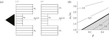
, i.e. stronger reverse flow, promotes greater global mode growth rate (see figure 1).
-
(b) Density ratio of the unburned reactants (located in the outer flow) to that of the burned products (located in the wake),
${\it\rho}_{u}/{\it\rho}_{b}$
. Lower density ratios promote greater global mode growth rates. A low density ratio is the result of low exothermicity of combustion and/or significant reactant preheat. -
(c) Degree of offset between the shear layer and density point of inflection. Greater offsets promote higher global mode growth rates by altering the balance between baroclinic induced vorticity and shear induced vorticity.


These first two results are summarized in a model calculation result shown in figure 1, which plots iso-contours of the absolute growth rate as a function of backflow and density ratio.
(a) Model wake flow profiles and (b) absolute/convective stability instability map for the model base flow, parameterized by density ratio and backflow ratio, following Yu & Monkewitz (Reference Yu and Monkewitz1990). Contour levels of the non-dimensional absolute growth rate,
 ${\it\omega}_{0,i}D/(2u_{av})$
, are labelled on the plot, and the shaded region indicates absolute instability.

To summarize, while iso-density wakes become globally unstable at low Reynolds numbers, the wake density ratio acts as an important bifurcation parameter that, depending upon its value, can render high Reynolds number wakes to be globally stable or unstable (Huerre & Monkewitz Reference Huerre and Monkewitz1990; Anderson, Hertzberg & Mahalingam Reference Anderson, Hertzberg and Mahalingam1996; Godreche & Manneville Reference Godreche and Manneville1998; Schmid & Henningson Reference Schmid and Henningson2001). For example, typical density ratios for hydrocarbon flames fuelled by room temperature reactants are about 5–8, which causes the global wake mode to be damped in almost all applications. In contrast, low density ratios of 1.5–3 are typically achieved in cases with highly preheated flows, such as in cases where the reactants are highly compressed or vitiated, destabilizing the global wake mode. As noted above, the density ratio at which this bifurcation occurs is controlled by the ‘backflow ratio’ and shear-density layer offset.
The implications of the global/convective instability distinction are particularly significant in problems where the wake is forced. An important application where harmonic acoustic forcing of reacting wakes occurs is the thermoacoustic instability problem, where vortical structures excited by acoustic waves play important roles in the heat release feedback mechanism (Lieuwen & Yang Reference Lieuwen and Yang2005), as mentioned earlier. A globally stable, but convectively unstable system is quite sensitive to acoustic excitation (Huerre & Monkewitz Reference Huerre and Monkewitz1990). Indeed, it is well known that the strong vortices excited by the convectively unstable shear layer play a key role in causing the heat release oscillations leading to combustion instability (Smith & Zukoski Reference Smith and Zukoski1985; Yang & Culick Reference Yang and Culick1986; Poinsot et al. Reference Poinsot, Trouve, Veynante, Candel and Esposito1987; Hermanson & Dimotakis Reference Hermanson and Dimotakis1989; Yu, Trouve & Candel Reference Yu, Trouve and Candel1991; Soteriou & Ghoniem Reference Soteriou and Ghoniem1994). In contrast, a globally unstable system is a self-excited oscillator – it exhibits intrinsic self-excited oscillations. Globally unstable flows saturate to a limit cycle, and exhibit a highly nonlinear forced response character (Blevins Reference Blevins1977; Masselin & Ho Reference Masselin and Ho1985; Bellows, Hreiz & Lieuwen Reference Bellows, Hreiz and Lieuwen2008). Therefore, in the case of a globally stable flow, low amplitude acoustic excitation induces a proportional hydrodynamic response, while in a globally unstable flow it may not. In turn, this has important implications on which type of flow instabilities are involved in linear and nonlinear combustion instability mechanisms. Moreover, it suggests that simulating combustion instabilities in simplified combustors with high density ratio, convectively unstable flows will lead to completely different acoustic-hydrodynamic coupling processes than what may actually be occurring in the low flame density ratio conditions which generally occur in real applications.
This paper focuses in particular on harmonically forced, reacting wakes. Consider first the significant existing literature on unforced iso-density wakes (Naudascher & Rockwell Reference Naudascher and Rockwell1994). Broadband shear layer disturbances grow at a rate associated with the most rapidly amplified, natural spatial mode, leading to rollup into concentrated regions of vorticity, which pair as they convect downstream (Roshko Reference Roshko1976). For a shear layer in the presence of harmonic forcing, the pairing process is altered so that vortices merge in such a way as to render a strong forced response at the forcing frequency (Ho & Huang Reference Ho and Huang1982). For example, a train of vortices passing at three times the forcing frequency will tend to merge three at a time to match the forcing frequency. If the forcing frequency is much lower than the vortex passage frequency, a phenomenon called ‘collective interaction’ occurs. In this case, a large number of vortices are spatially localized and merged into one, much larger vortex (Ho & Nosseir Reference Ho and Nosseir1981).
In the wake problem, interaction of the two shear layers leads to collection of the small shear layer structures into much larger vortices whose sizes scale with the wake width, and which pass through the wake at the global mode frequency. However, just like the individual shear layers, a harmonically excited wake may adjust the passage frequency of these large vortices to match the excitation frequency (Blevins Reference Blevins1977; Provansal et al.
Reference Provansal, Mathis and Boyer1987). In a globally unstable flow, this phenomenon occurs through frequency locking (Bishop & Hassan Reference Bishop and Hassan1964; Ferguson & Parkinson Reference Ferguson and Parkinson1967; Tanida, Okajima & Watanabe Reference Tanida, Okajima and Watanabe1973; Griffin & Ramberg Reference Griffin and Ramberg1976; Stansby Reference Stansby1976; Barbi et al.
Reference Barbi, Favier, Maresca and Telionis1986). Frequency locking occurs with sufficiently high forcing amplitude, whose value is a function of the relative values of the global mode and forcing frequencies,
 $f_{n}$
and
 $f_{f}$
, respectively. Thus, when these flows are forced at low amplitudes, they tend to oscillate primarily at the global mode frequency,
 $f_{n}$
, as if they are unforced, but oscillate at the forcing frequency,
 $f_{f}$
, when forced at high amplitudes. Studies also show that frequency locking alters the topology of the flow dynamics (Tanida et al.
Reference Tanida, Okajima and Watanabe1973; Griffin & Ramberg Reference Griffin and Ramberg1976; Konstantinidis & Balabani Reference Konstantinidis and Balabani2007). For example, Konstantinidis & Balabani (Reference Konstantinidis and Balabani2007) demonstrate that symmetric forcing causes the near wake to respond with a varicose arrangement of coherent structures, which pass at the forcing frequency. Eventually, these structures stagger into a sinuous configuration as they convect downstream. This staggering occurs at some distance downstream of the bluff body which depends on the forcing amplitude as well as the proximity of the forcing frequency to the global mode frequency.
The literature on forced wakes with density stratification is substantially more limited. While a variety of studies addressing various aspects of combustion instabilities in bluff body stabilized flames exist, the authors are not aware of systematic investigations of harmonically forced, reacting, high Reynolds number wakes that consider the problem from the perspective of modern hydrodynamic stability analysis. This problem has important additional degrees of freedom relative to the iso-density wake, as the density ratio acts as an important hydrodynamic global stability bifurcation parameter, and the unforced absolute stability analysis suggests that the forced flow dynamics of the low, mid and high density ratio wakes could be quite different. In addition to the flow dynamics, the axial distribution of the unsteady heat release is another important quantity which also is substantively influenced by whether the dominant vortex structures are symmetrically configured across the flow centreline (where the disturbances in heat release of the two flame branches are in phase), or asymmetrically staggered in a sinuous configuration (where the heat release of the two flame branches are out of phase). Despite its importance for the response of flames to acoustic forcing, the unsteady heat release response characteristics of reacting wakes have not been systematically investigated, in particular as a function of the density ratio and the forcing frequency relative to the global mode frequency.
This paper investigates the harmonically forced response of reacting wakes where the axial forcing, by its very nature, excites a varicose mode of the flow. Simultaneously, the most rapidly amplified mode is sinuous. Therefore, multiple flow response scenarios are possible in a given flow at different axial locations and frequency ratios that are detailed in the paper. To the best of the authors’ knowledge, this is the first systematic study of the forced response of a reacting bluff body flow field whose global instability behaviour is itself a parameter.
2. Experimental setup and data analysis
2.1. Experimental facility
This section describes the experimental facility in which flame density ratio and lip velocity can be independently varied. By varying the density ratio, the hydrodynamic global mode growth rate can be systematically varied. During a density ratio sweep, the flow evolves from a globally stable to a globally unstable system that exhibits intrinsic oscillations. In addition, by varying the lip velocity, the global mode frequency can be varied relative to the fixed forcing frequency. Great care is taken to operate this combustor well away from blowoff boundaries, where additional flame and flow dynamics can occur (Shanbhogue et al. Reference Shanbhogue, Husain and Lieuwen2009a ; Chaudhuri et al. Reference Chaudhuri, Kostka, Renfro and Cetegen2010a ,Reference Chaudhuri, Kostka, Tuttle, Renfro and Cetegen b ).
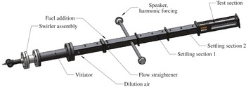
The experimental rig, shown in figures 2 and 3, consists of two premixed, methane-air combustors in series. The first combustor is used to vitiate the flow and raise its temperature. The second, bluff body stabilized combustor, consists of a rectangular section with a bluff body spanning the width of the combustor, creating a nominally 2-D flow. The aspect ratio of bluff body height to chamber width is 0.15. This combustor has quartz windows for optical access from all four sides. The bluff body used in the test section, shown in figure 3(b) has a 2-D ballistic shape. Additional fuel and air injection sources are located between the two burners, allowing substantial flexibility in density ratio and lip velocity. Further details of this facility and its design are provided in Emerson et al. (Reference Emerson, O’Connor, Juniper and Lieuwen2012).
Schematic of the atmospheric pressure, vitiated, bluff body rig.

Drawings of (a) the test section and (b) the bluff body.

A function generator is used to generate the forcing signal, which is then amplified and used to drive two loudspeakers which are mounted to tubes that enter the combustor one metre upstream of the test section. Because the first transverse mode of this rig has a frequency of 5000 Hz, multi-dimensional disturbances are evanescent and decay quickly, so that the acoustic excitation in the test section is effectively planar. The forcing frequency is held fixed at 515 Hz for all experiments, since a strong forced response is possible here, which is an important consideration in the
 $50~\text{m}~\text{s}^{-1}$
flow conditions.
Data acquisition parameters were optimized to effectively eliminate spectral leakage from the forcing frequency, a particularly important consideration when the global mode frequency and forcing frequency are close. This is accomplished by using a boxcar spectral windowing function, and setting the forcing frequency,
 $f_{f}$
, sampling frequency,
 $f_{sample}$
and number of samples,
 $N_{s}$
, such that (2.1) is satisfied (Lieuwen et al.
Reference Lieuwen, Rajaram, Neumeier and Nair2002). In essence, this equation ensures that an integer number of cycles,
 $j$
, of the forced response are sampled.
 $$\begin{eqnarray}f_{f}=jf_{sample}/N_{s}.\end{eqnarray}$$
The uncertainty in the relative forcing and sampling frequencies is about
 $10^{-6}~\text{Hz}$
. As such, when using a boxcar window, the bias errors in the spectral estimate due to leakage one frequency bin away from
 $f_{f}$
is of the order of
 $10^{-12}\,\%$
. Note that such a discrete frequency excitation problem is one instance where the boxcar window function is superior to other windows. These considerations are important when analysing the impact of narrowband forcing upon other frequencies, such as the power in the global mode, as it is otherwise difficult to differentiate leakage induced bias errors from physical changes in the spectral power of the phenomenon of interest.
The test matrix is designed to independently adjust the air flow rates and equivalence ratios in the two burners to achieve a velocity sweep at a fixed density ratio, for a number of different density ratios. The velocity sweep causes a sweep in global mode frequency. In these experiments, the test section inlet temperature (after vitiation and addition of secondary air and fuel) was varied from 770 to 1200 K; this enabled us to vary the density of the reactants,
 ${\it\rho}_{u}$
, as well as the density ratio across the flame,
 ${\it\rho}_{u}/{\it\rho}_{b}$
. The test section equivalence ratio was held in the range
 $0.70<{\it\phi}<0.75$
, and the adiabatic flame temperature remained in the range
 $1950~\text{K}<T_{b}<2030~\text{K}$
.
Bluff body lip velocities quoted in this paper are calculated using the formula
 $U_{lip}={\dot{m}}/({\it\rho}_{lip}A_{lip})$
, which is an average axial flow velocity. The density for the lip velocity calculation was determined from the temperature measured just before the test section and the gas composition of the secondary air and fuel adiabatically mixed with the equilibrium vitiated gas. An equilibrium gas solver was then used to calculate the adiabatic density ratio across the test section flame. The area,
 $A_{lip}$
, is the cross-sectional area of the flow at the plane of the bluff body trailing edge (accounting for the blockage of the bluff body).
The primary experimental diagnostics consisted of high speed, line of sight integrated (along the bluff body span) imaging of flame chemiluminescence, and high speed particle image velocimetry (PIV). High speed chemiluminescence imaging was performed with a high speed CMOS camera with
 $21.7~{\rm\mu}\text{m}$
pixels, operating at a 5000 Hz frame rate and 768
 $\times$
384 pixel resolution. The exposure time was
 $1/5000~\text{s}$
. The camera was outfitted with a 135 mm lens at
 $f/2.8$
, with a magnification of 1:17.1, such that a 286 mm
 $\times$
80 mm region of the test section was imaged on 768
 $\times$
215 pixels. This region of the test section spanned from the bluff body trailing edge to 15 bluff body diameters downstream. The flame was imaged through a bandpass filter centred at 434 nm, with 90 % transmission between 425.5 and 442.5 nm. A total of 4000 images was acquired in each run. The chemiluminescence imaging was used to characterize the dynamical displacement of the flame, as well as the unsteady heat release (Gaydon & Wolfhard Reference Gaydon and Wolfhard1970) of the flame. The displacement of the flame was quantified by first performing edge detection on the chemiluminescence images. The threshold based edge detection scheme used Otsu’s method (Otsu Reference Otsu1975) to identify a threshold intensity contour level. At each axial position, the flame edge displacement,
 $L^{\prime }$
, is defined as the instantaneous transverse position of this contour level, relative to its mean transverse position (see figure 5
b).
Mie scattering images for high speed PIV were obtained as follows. The flow was seeded with
 $5~{\rm\mu}\text{m}$
 $\text{Al}_{2}\text{O}_{3}$
particles, chosen due to their durability in reacting flows and their high refractive index (Melling Reference Melling1997). This particle size was chosen because it is large enough to slow down accumulation on and clouding of the test section windows, while retaining a sufficiently small Stokes number to accurately track the flow at the frequencies of interest. Following the work by Mei (Reference Mei1996), the Stokes number calculated for this flow and seed particle combination was 0.015. This Stokes number is calculated using a kinematic viscosity of
 $3\times 10^{-4}~\text{m}^{2}~\text{s}^{-1}$
, and oscillation frequency of 850 Hz (roughly the highest global mode frequency encountered). This Stokes number is comfortably below the cutoff Stokes number for solid particles in air (Mei Reference Mei1996), which is in the range of 0.02–0.04 and would correspond to a frequency of at least 1500 Hz.
The particle-laden flow was illuminated with a double-pulsed Nd:YLF laser, with wavelength of 527 nm, pulse duration of 100 ns and
 $4~\text{mJ}~\text{pulse}^{-1}$
pulse energy. Each of the two lasers in the double-pulsed system is operated at 5000 Hz. The laser beams were expanded with a
 $-50~\text{mm}$
cylindrical lens into an expanding sheet, and the sheet was shaped with a 750 mm cylindrical lens to have a nominally 4 mm thickness. An expanding sheet was chosen instead of a collimated sheet because of the large test area. The time delay,
 $\text{d}t$
, between the two illuminating laser pulses of a given pair was
 $12~{\rm\mu}\text{s}$
. The short
 $\text{d}t$
is responsible for much of the velocity uncertainty, as discussed below. Mie scattering image pairs were captured by a high speed CMOS camera with
 $20~{\rm\mu}\text{m}$
pixels. The camera was outfitted with a 55 mm lens, with aperture at
 $f/5.6$
. The camera was operated with a pixel resolution of 640
 $\times$
448, with image pairs acquired at a frame rate of 5 kHz. The optical configuration produced a magnification of 1:12.5, such that the measurement domain covered a 640 pixel
 $\times$
320 pixel region of the CMOS chip, which corresponded to a region of the combustor that was roughly 160 mm long in the axial direction and 80 mm wide in the transverse direction. The measurement plane was located at the centrespan of the bluff body. The diffraction limited spot size for this configuration was
 $7~{\rm\mu}\text{m}$
. Slight defocusing, together with the natural aberration and imperfections of the imaging optics, distributed the scattered light from the particles over a nominal 3 pixel diameter. A bandpass optical filter was placed in front of the camera in order to reject the majority of flame and other background luminosity. The filter passband is centred at 527 nm and has a transmission of greater than 93 % from 517 to 537 nm.
Velocity vectors were computed from the Mie scattering image pairs using a digital cross-correlation algorithm (Willert Reference Willert1991) with a multi-pass approach (Soria Reference Soria1996) and 2-D Gaussian subpixel interpolation (Willert Reference Willert1991). The multi-pass analysis consisted of a single pass with 64
 $\times$
64 pixel interrogation windows and 50 % overlap between interrogation windows, followed by 2 passes with 32
 $\times$
32 pixel interrogation windows and 50 % overlap between the interrogation windows. The spacing between vectors was 4 mm.
Post-processing algorithms were used to discard and replace a small number of spurious vectors, and to validate the PIV data. First, any velocity vector with an axial component outside of a
 $20\,\pm \,90~\text{m}~\text{s}^{-1}$
range or a transverse component outside of a
 $\pm 45~\text{m}~\text{s}^{-1}$
range was discarded. These ranges were based on the expected range of mean axial and transverse velocities, and additionally, they conservatively accommodate coherent structures with unsteady velocity on the order of the nominal
 $50~\text{m}~\text{s}^{-1}$
lip velocity. Next, any velocity vector whose velocimetry calculation had a peak correlation coefficient less than 0.2 was discarded and a local validation method discarded neighbouring vectors whose ratio of difference to average velocity magnitude was greater than 20 % of the r.m.s. of the nearest neighbours. This threshold is consistent with values recommended in the literature (Nogueria, Lecuona & Rodriguez Reference Nogueria, Lecuona and Rodriguez1997). In all, less than 1 % of the total velocity vectors were discarded and their values filled with the instantaneous average of neighbouring vectors.
The PIV measurement was calibrated by imaging a black anodized aluminum calibration plate with a laser etched pattern, which was located coincidently with the laser light sheet. The laser etched pattern consisted of a regularly spaced grid of crosses, composed of 0.3 mm thick lines, with spacing of 6 mm and with positional uncertainty of 0.004 %. The spatial coordinates of the Mie scattering images and resultant velocity fields were mapped to this grid. The worst-case calibration error was estimated to be one pixel over the large 160 mm calibration plate, which would result in a small 0.2 % bias error. The phase jitter between the pair of laser illumination pulses was measured to be on the order of nanoseconds, which is significantly less than the relatively long 100 ns duration at half-maximum of each illumination. Therefore, the duration of the laser illumination dominates the temporal measurement uncertainty, which is less than 1 % of the time delay between the pair of illumination pulses. Peak locking during subpixel interpolation (Fincham & Spedding Reference Fincham and Spedding1997), combined with the relatively short
 $\text{d}t$
, was estimated to provide a velocity uncertainty of 4 %. In/out of plane motion dominates the velocity uncertainty over much of the measurement domain, and increases with distance from the measurement centre (located at
 $x/D=4$
). For example, at axial positions 20 mm from the measurement centre (i.e. at
 $x/D=3$
and
 $x/D=5$
), this uncertainty is 5 %. As the measurement position moves to the extreme axial extents of the measurement, i.e. to
 $x/D=0$
and
 $x/D=8$
, this uncertainty increases linearly to 20 %. However, the uncertainty due to in and out of plane motion applies to turbulence and secondary instabilities in this flow, but does not directly impact the nominally 2-D hydrodynamic motion and time-averaged velocity field of interest. Finally, following the seeding particle Stokes number discussion above, the seeding particles are expected to respond at the forcing frequency with 92 % of the flow response amplitude and with less than a
 $20^{\circ }$
phase delay.
The PIV data was supplemented with two component laser Doppler velocimetry (LDV) (Durst, Melling & Whitelaw Reference Durst, Melling and Whitelaw1976) and a single wire constant temperature hot wire anemometer, to characterize the flow upstream of the test section. The LDV measurement was obtained at the bluff body trailing edge by scanning the flow transversely in steps of 0.1 mm. LDV was selected for measurement in this region because it is well suited to fine spatial resolution, and has less trouble than PIV with laser light reflecting from the bluff body. The LDV measurement captured the streamwise,
 $u$
, and transverse,
 $v$
, velocity components at the inflow. Seeding material consisted of
 $5~{\rm\mu}\text{m}$
aluminum oxide, whose flow tracking fidelity characteristics were discussed previously. For each measurement volume, data acquisition was limited to either 30 s or 5000 s counts, whichever came first. The acquisition channel used for axial velocity measurements used a laser wavelength of 514.5 nm, a fringe spacing of
 $7.9196~{\rm\mu}\text{m}$
, a beam waist of
 $70.19~{\rm\mu}\text{m}$
and a Bragg cell frequency of 40 MHz. The resulting low and high velocity limits were
 $-24~\text{m}~\text{s}^{-1}$
and
 $119~\text{m}~\text{s}^{-1}$
, respectively. The acquisition channel used to measure the transverse velocity used a laser wavelength of 488 nm, a fringe spacing of
 $7.5117~{\rm\mu}\text{m}$
, a beam waist of
 $66.57~{\rm\mu}\text{m}$
and a Bragg cell frequency of 40 MHz. For this channel, the low and high velocity limits were
 $-68$
and
 $68~\text{m}~\text{s}^{-1}$
, respectively. Both channels had a focal length of 300 mm, a beam separation of 19.5 mm, a beam diameter of 2.8 mm and used a 20 MHz high pass filter. The measurement volume for LDV was
 $150~{\rm\mu}\text{m}$
long, aligned in the axial direction, and
 $80~{\rm\mu}\text{m}$
in diameter.
The hot wire measurement was obtained in the optically inaccessible region upstream of the test section. This measurement was used to estimate the inflow conditions, but was limited to non-vitiated conditions with the test section removed. The hot wire measurement scanned the channel in steps of 5 mm, with 10 000 samples recorded at each position at an acquisition rate of 8186 Hz.
2.2. Linear stability calculation approach
This section introduces the background and methodology behind the stability analysis, which closely follows Juniper, Tammisola & Lundell (Reference Juniper, Tammisola and Lundell2011). These analyses use measured, time-averaged velocity profiles as inputs into the stability analysis in order to obtain insight into the role of linear processes in disturbance growth. A number of studies have similarly used the time-averaged velocity profiles from turbulent flows as inputs to laminar flow stability analyses to make predictions about flow stability behaviour such as linear disturbance amplification rates, nonlinear saturation and disturbance frequencies (Barkley Reference Barkley2006; Meliga, Pujals & Serre Reference Meliga, Pujals and Serre2012; Mettot, Sipp & Bezard Reference Mettot, Sipp and Bezard2014). This ‘quasi-laminar’ approach is taken in this study as well, but the authors caution that a number of questions remain around the bounds of applicability of such analyses.
First, the measured base flow is inserted into the linearized continuity and 2-D Navier–Stokes equations, which results in a system of PDE with the linear velocity and pressure perturbations as state variables. This system of PDE is reduced to ODE by projecting the state variables onto a basis of Fourier modes in time and axial position. Next, the system of ODE is reduced to a coupled system of algebraic equations, expressed as a generalized eigenvalue problem by projecting the state variables onto Chebyshev polynomials in the transverse dimension. Boundary conditions at the wall and the flow centreline are included in this algebraic system. At the confining wall, the boundary conditions enforce the no-slip and impermeability conditions. The boundary conditions at the flow centreline establish either a varicose or sinuous mode. At this location, the varicose mode has zero transverse velocity and zero cross-stream gradients of pressure and axial velocity. In contrast, the sinuous mode has centreline boundary conditions of zero axial velocity and pressure, and zero cross-stream gradient of transverse velocity. This generalized eigenvalue problem is defined for a given base flow and complex wavenumber,
 $k=k_{r}+\text{i}k_{i}$
. Its eigenvalue is the complex frequency,
 ${\it\omega}={\it\omega}_{r}+\text{i}{\it\omega}_{i}$
, and its eigenvector gives the radial dependence of the state variables,
 $u$
,
 $v$
and
 $p$
. The spatial stability analysis is solved by first performing a temporal stability analysis, which computes the dependence of the complex frequency on the real valued wavenumber,
 ${\it\omega}(k_{r})$
. The temporal analysis is used to identify the most amplified solution branch, after removing high frequency non-physical solutions. The temporal stability analysis defines a path through the complex
 ${\it\omega}$
plane, with a corresponding path along the real
 $k$
axis. Integration of the solution along this frequency-domain path would represent an inverse Fourier transform. This inverse Fourier transform would provide the time domain solution for the flow, if it were excited with the broadband dynamics defined by the values of
 $k$
and
 ${\it\omega}$
that lie along the integration path.
In order to construct a meaningful spatial stability analysis, this integration contour is deformed to lie along the real
 ${\it\omega}$
axis, following the procedure outlined by Huerre & Monkewitz (Reference Huerre and Monkewitz1985). The resulting path along the real
 ${\it\omega}$
axis has a corresponding path through the complex
 $k$
plane. To conclude the local spatial stability analysis, the complex wavenumber that corresponds to the real valued forcing frequency is extracted from this path. The negative of the imaginary part of this wavenumber represents the linear spatial growth rate of harmonic disturbances travelling in the positive
 $x$
(downstream) direction. These local analyses are used to estimate the axial dependence of the local spatial growth rate,
 $k(x,f)$
.
The process outlined above is performed as a local stability analysis, and is repeated at each axial position. In real flows, the time-averaged flow evolves axially. Therefore, following Chrighton (Reference Chrighton1973), the Wentzel–Kramer–Brillioun–Jeffreys (WKBJ) approximation is used to assemble the local stability analyses into a growth envelope,
 ${\it\zeta}(x,f)$
, which is a function of axial position and the frequency of interest using the following expression.
 $$\begin{eqnarray}{\it\zeta}(x,f)=\exp \left\{\text{i}\int _{0}^{x}k(x^{\prime },f)\,\text{d}x^{\prime }\right\}.\end{eqnarray}$$
This approximation is valid for weakly non-parallel flows.
3. Baseline unforced results
3.1. Inlet conditions
This section provides the properties of the velocity field at the inlet of the test section. A hot wire anemometer, under non-vitiated conditions, was traversed across the channel height,
 $H$
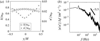
, to measure the mean velocity profile and turbulence properties upstream of the bluff body. The hot wire measurements do not resolve the thin boundary layers of the channel walls. Figure 4(a) shows the mean axial velocity and r.m.s. velocity profiles across the channel. The results show that the mean velocity in the channel is relatively uniform, and is roughly
 $3/4$
of the bluff body lip velocity (due to acceleration through the blockage of the bluff body). The turbulence intensity ranges from roughly 1 % in the channel centre to 3 % near the walls. Figure 4(b) shows the turbulent energy spectrum at the channel centreline just upstream of the bluff body.
Hot wire measurements in unvitiated, unforced conditions with
 $u_{lip}=50~\text{m}~\text{s}^{-1}$
. Results show (a) mean axial velocity and unsteady velocity profiles across the channel just upstream of the bluff body, with dashed line indicating
 $\bar{u}=0.75u_{lip}$
and (b) turbulent energy spectrum measured at the centreline of the channel just upstream of the bluff body.

LDV measurements in the channel between the bluff body and the confining wall, at the plane of the bluff body trailing edge, were obtained to measure the thin shear layer separating from the trailing edge of the bluff body. Near the surface of the bluff body, the shear layer is 1 mm thick with 15–20 % turbulence intensity over the range of conditions reported in the paper. Outside of this boundary layer, the velocity profile (in the channel) is uniform with 8–10 % turbulence intensity. At this axial position, the contribution of the global mode to the turbulent kinetic energy is less than 1 %. These shear layer measurements, along with further characterization of the time-averaged flow, are reported in more detail in previous work (Emerson et al. Reference Emerson, O’Connor, Juniper and Lieuwen2012).
3.2. Density ratio influences
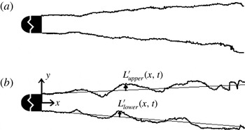
This section reviews the dynamics of the unforced flame response, summarizing results from Emerson et al. (Reference Emerson, O’Connor, Juniper and Lieuwen2012). The coordinate system and nomenclature used for flame edge displacement are presented in figure 5(b). For brevity,
 $L^{\prime }$
will be used to denote the upper flame branch displacement; when both the upper and lower flame branches are considered together, the subscripts lower and upper are added.
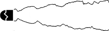
Instantaneous edges of unforced flames at (a)
 ${\it\rho}_{u}/{\it\rho}_{b}=2.5$
, (b)
 ${\it\rho}_{u}/{\it\rho}_{b}=1.9$
, extracted from chemiluminescence images.

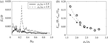
(a) Flame edge displacement spectra for two density ratios, (b) dependence of the global mode amplitude on density ratio, shown for the flame edge displacement and the centreline transverse velocity. All results are at
 $x/D=3$
.

Flame edge spectra,
 $\hat{L}(x,f)$
, are presented in figure 6(a) for high and low density ratios. Note that the low density ratio flame has strong, narrowband energy centred around
 $St_{D}=0.24$
, as opposed to the much more spectrally distributed energy in the high density ratio flame. This is indicative of the presence of a global instability for the low density ratio cases (this peak is not associated with an acoustic mode of the chamber, as evidenced by its frequency scaling linearly with flow velocity). In order to quantify the limit cycle amplitude of the global mode, the integrated power under the spectral peak between Strouhal numbers of 0.20 and 0.28 is computed as a function of density ratio and converted into a r.m.s. amplitude using Parseval’s theorem, shown in (3.1) for a time series
 $s(t)$
with duration
 $T$
and power spectrum
 $|{\hat{s}}(f)|^{2}$
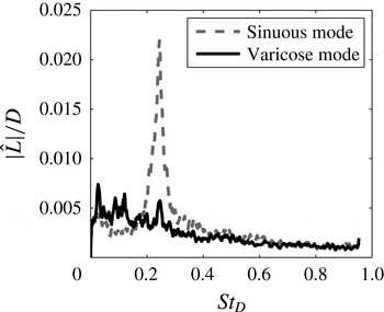
. Figure 6(b) plots the flame displacement and transverse velocity amplitude as functions of the density ratio, illustrating its strong influence on the amplitude of the global mode. Figure 7 presents spectra of the flame edge displacement decomposed into sinuous and varicose components, demonstrating that the global mode at
 $St_{D}=0.24$
is dominated by sinuous disturbances.
 $$\begin{eqnarray}s_{rms}^{\prime }=\sqrt{\frac{1}{T}\int |{\hat{s}}(f)|^{2}\,\text{d}f}.\end{eqnarray}$$
Decomposition of flame edge displacement into sinuous and varicose disturbances for
 ${\it\rho}_{u}/{\it\rho}_{b}=1.9$
,
 $x/D=3$
.

4. Forced flow response results
This section presents forced response characteristics of the flow. The forcing amplitude is denoted as
 $A_{f}$
, which is the ratio of the acoustic particle displacement amplitude to the bluff body diameter, calculated as
 $A_{f}=|u_{lip}^{\prime }(f_{f})|/(2{\rm\pi}f_{f}D)$
, where
 $u_{lip}^{\prime }$
is the unsteady axial velocity at
 $x/D=0$
and
 $y/D=1$
. The forcing corresponds to a particle displacement amplitude of 0.5 mm, or
 $A_{f}=0.2$
. This value of forcing amplitude corresponds roughly to an acoustic velocity of 3 % of the bluff body lip velocity. In order to estimate
 $u_{lip}^{\prime }$
, the narrowband unsteady axial velocity was extracted from the PIV measurement, at the forcing frequency, at the axial position of the bluff body trailing edge and a transverse position half-way between the bluff body surface and the confining wall. At this position, the narrowband power spectral density of the forced motion is two orders of magnitude greater than the broadband background turbulence. Additionally, the sensitivity of the results to the forcing amplitude was investigated by repeating the study at four different forcing amplitudes, which spanned a factor of 4 and which showed no influence on the qualitative results presented in this paper. A brief summary of the influence of forcing on the time-averaged flow is presented in appendix A, showing that forcing reduces the recirculation zone length. External forcing strongly influences the rollup of the separating shear layers, and how they subsequently merge and interact to form larger-scale structures. These unsteady structures then form wrinkles in the flame front (Schuller et al.
Reference Schuller, Ducruix, Durox and Candel2002; Shanbhogue Reference Shanbhogue2008; Shanbhogue et al.
Reference Shanbhogue, Shin, Hemchandra, Plaks and Lieuwen2009b
). Figure 8 illustrates flame edges of an unvitiated, high density ratio (
 ${\it\rho}_{u}/{\it\rho}_{b}=6$
) flame. The image shows a flame that is wrinkled by symmetric vortical structures for the first few bluff body diameters downstream, which are excited by the forcing and amplified by a convectively unstable flow. This illustrates the forced response that is typical of most non-preheated laboratory bluff body combustors. However, at low density ratios, the hydrodynamic global mode becomes weakly damped or unstable, which is expected to significantly change the forced response characteristics. This section will show that the forced response characteristics of low density ratio wakes exhibit a complicated mix of sinuous and varicose disturbance features, and that these characteristics are highly sensitive to the proximity of the forcing frequency to the global mode frequency and the axial location.
Representative instantaneous flame edge from forced flame, conditions were
 $u_{lip}=15~\text{m}~\text{s}^{-1}$
, forcing frequency of
 $f_{f}=515~\text{Hz}$
, equivalence ratio of
 ${\it\phi}=0.7$
and density ratio of
 ${\it\rho}_{u}/{\it\rho}_{b}=6$
.

This paper analyses two nominal modes of flow oscillation: one with a sinuous spatial structure, and one with a varicose spatial structure. To quantify the energy in these two modes, the analysis begins by decomposing the flow dynamics into these two modes according to (1.3). Next, the energies of the sinuous and varicose transverse velocity fluctuations are integrated across the transverse dimension in order to define an energy measure that is a function of axial location and frequency only.
 $$\begin{eqnarray}\left.\begin{array}{@{}c@{}}\displaystyle e_{s}(f,x)=\int _{0}^{H}|\hat{v}_{s}(x,y,f_{f})|^{2}{\rm\Delta}f\,\text{d}y\\ \displaystyle e_{v}(f,x)=\int _{0}^{H}|\hat{v}_{v}(x,y,f_{f})|^{2}{\rm\Delta}f\,\text{d}y.\end{array}\!\!\right\}\end{eqnarray}$$
In (4.1),
 ${\rm\Delta}f$
represents the bandwidth of a single frequency bin.
4.1. Basic flow response features
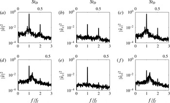
Figure 9 shows typical flow power spectra at two forcing frequencies. The three columns show the spectra of the transverse velocity (figure 9
a,d) and its decomposition into varicose (figure 9
b,e) and sinuous (figure 9
c,f) disturbances. The first row shows results for a forcing frequency right at the global mode frequency, and the second row for a forcing frequency 30 % higher than the global mode frequency. The spectra show clear narrowband energy at the forcing frequency (
 $f/f_{f}=1$
), at harmonics of the forcing frequency and at the global mode frequency (at
 $St_{D}=0.24$
). For example, figure 9(f) shows a case where the sinuous mode contains significant energy at both the forcing and global mode frequency. Figure 9(b) shows a case where the varicose mode contains significant energy at the forcing frequency and its first harmonic. When the flow is near the global stability boundary (i.e. at low
 ${\it\rho}_{u}/{\it\rho}_{b}$
), such multi-modal behaviour is typical of the forced response dynamics.
The spectra in figure 9 reveal general trends about each of the spectral features. First, just as in the unforced case (e.g. see figure 7), the global mode at
 $St_{D}=0.24$
is almost completely composed of sinuous motions; very little energy at this frequency is present in the varicose mode. Second, the forced response (at
 $f/f_{f}=1$
) is composed of both sinuous and varicose motions. Third, while the first harmonic of the forced response (at
 $f/f_{f}=2$
) is present in both varicose and sinuous modes, its amplitude is similar to the fundamental’s amplitude only in the varicose mode when the system is forced at
 $f_{n}/f_{f}=1$
(referred to as resonant forcing in the rest of this paper). The rest of this paper focuses on how these spectral features evolve as functions of axial position,
 $x/D$
, and proximity of the forcing frequency to the global mode frequency,
 $f_{n}/f_{f}$
.
(a,d) Shows typical forced flow power spectra at
 $x/D=3$
,
 ${\it\rho}_{u}/{\it\rho}_{b}=1.9$
. (b,e) Shows same power spectra but for varicose mode only, and (c,f) shows same power spectra but for sinuous mode only. (a–c) Shows results for
 $f_{n}/f_{f}=1.0$
, (d–f) shows results for
 $f_{n}/f_{f}=1.3$
.

Forced flame and flow spectra for
 ${\it\rho}_{u}/{\it\rho}_{b}=1.9$
,
 $x/D=3$
, showing a sweep (a–o) of the global mode frequency from
 $f_{n}/f_{f}=0.7$
(a–c), 9 (d–f), 1.2 (g–i) to 1.3 (m–o). (a,d,g,j,m) Instantaneous line of sight chemiluminescence with phase-averaged iso-vorticity contours overlaid. (b,e,h,k,n) Transverse velocity spectra at
 $x/D=3.0$
. The ● symbol hovers over the global mode at
 $f_{n}$
. The solid lines in the (c,f,i,l,o) are envelopes of the forced response energy, decomposed into sinuous and varicose modes. These envelopes are laid over shaded regions, which are linear growth envelopes (shaded over a range of uncertainty) from local stability analysis.

Figure 10 summarizes the effect of
 $f_{n}/f_{f}$
on the flow spectra, the flame structure and the forced flow topology. The rows in figure 10 from (a–o) sweep the ratio of the global mode to forcing frequency, from
 $f_{n}/f_{f}=0.7$
to
 $f_{n}/f_{f}=1.3$
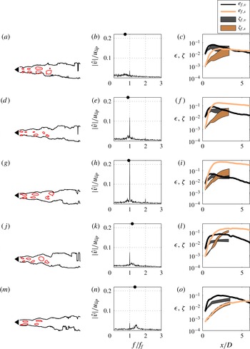
. The first column shows instantaneous flame images at the different forcing frequencies. The flame serves as a convenient form of flow visualization near the bluff body but there are important precautions for interpreting its behaviour farther downstream. Specifically, its behaviour reflects not only the local flow dynamics but also the dynamics from all upstream positions (Boyer & Quinard Reference Boyer and Quinard1990; Lieuwen Reference Lieuwen2012); i.e. it exhibits ‘memory’, which renders its interpretation farther downstream more complex. This memory effect has significant influence on its heat release dynamics, as discussed later in § 5.3. Iso-vorticity contours are also overlaid on the flame images, providing an image of the ensemble-averaged flow topology. The iso-vorticity contours are obtained by phase-averaging 400 instantaneous velocity measurements at the same phase as the flame image. The contour levels were hand-selected to illustrate the spatial distribution of coherent structures. The figure clearly shows the strong varicose flow and flame disturbance fields at global mode frequencies much lower than the forcing frequency, and the strong sinuous motions when
 $f_{n}\approx f_{f}$
.
Figure 10(b,e,h,k,n) shows flow spectra at a fixed axial position for the same frequency sweep test conditions. As
 $f_{n}/f_{f}$
increases, the broader hump associated with the global mode at
 $St_{D}=0.24$
and the much narrower peak at
 $f_{f}$
clearly move across each other. Note the strong resonant amplification of the narrowband forced response (the ordinate scales are kept consistent for all values of
 $f_{n}/f_{f}$
) when
 $f_{n}/f_{f}\approx 1$
, and the appearance of the harmonic of the forcing frequency at
 $f/f_{f}=2$
.
The solid lines plotted in figure 10(c,f,i,l and o) show the axial development of the energy in the sinuous and varicose disturbance fields at
 $f/f_{f}=1$
using (4.1). The shaded areas on these plots represent linear stability calculations, which are discussed in the next section. The figure shows that the acoustic forcing initially deposits energy in the varicose mode, as would be expected for this axially forced configuration, evidenced by this mode’s dominance near the bluff body for all cases. The energy in the sinuous mode also rises with downstream distance, but starting from a smaller value. This growth is expected, since both the sinuous and varicose modes are spatially amplified, as shown later in § 4.2. The relative growth in energy of these two disturbance modes is, however, strongly dependent upon
 $f_{n}/f_{f}$
. In particular, when
 $f_{n}\approx f_{f}$
, the sinuous mode grows very rapidly and quickly dominates the overall disturbance energy. Thus, the input acoustic disturbance energy quickly moves into sinuous disturbances under resonant conditions. At non-resonant conditions, the forced response energy remains in the varicose mode for a larger axial duration, although the sinuous mode may eventually dominate at some downstream axial location, quantified later.
An important question in regards to the growth of the sinuous and varicose disturbances is the relative roles of linear and nonlinear effects in their axial development, as well as the degree of their nonlinear interaction. For example, can the eventual dominance of the sinuous mode in the resonant case be explained purely by linear instability arguments due to the rapid linear spatial growth rates of slight asymmetries in the excitation field, or is its growth associated with the nonlinear transfer of energy from the varicose mode which is directly excited? The next two sections further examine the role of linear and nonlinear processes in the phenomena shown above. The analysis will show that the two disturbance modes initially grow independently of each other, and that linear processes are responsible for the much faster growth of the sinuous mode relative to the varicose mode. However, the sinuous mode begins to extract energy from the varicose mode farther downstream.
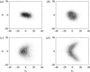
To separately investigate linear and nonlinear effects, figure 11 plots phase portraits (as scatter plots) of the instantaneous relationship between the sinuous and varicose disturbances at fixed axial locations. A positive value for the varicose mode corresponds to flow moving away from the centreline. Non-zero values of the sinuous mode indicate that the flow is washing across the centreline, either towards the upper channel wall (positive values) or towards the lower wall (negative values). Figure 11(a,b) shows phase portraits at an axial position of
 $x/D=1$
for cases without and with resonant amplification, respectively. The case without resonant amplification, shown in figure 11(a), exhibits a flattened shape due to the low amplitude of sinuous motion. In general, the analysis of all cases at
 $x/D\leqslant 1$
shows no correlation between the sinuous and varicose motions. At this condition, the sinuous and varicose disturbances are uncorrelated with each other, which therefore suggests that their spatial evolutions simply reflect independent linear amplification processes. Figure 11(c,d) shows phase portraits for the same conditions, but farther downstream at
 $x/D=3$
. In particular, figure 11(d) presents a phase portrait from
 $x/D=3$
for a case with clear resonant amplification, and shows a phase-coupled relationship between the sinuous and varicose disturbances. Interestingly, this trajectory is not circular or ovular, which would be the case for superposition of two synchronized harmonic signals. Rather, the varicose mode completes two cycles for every sinuous cycle, a manifestation of the prominent harmonic (
 $f=2f_{f}$
) in the spectrum for the
 $f_{n}/f_{f}=1$
case. The behaviour of the harmonic is discussed further in the next section and appendix B.
Phase portraits of the varicose mode energy plotted as a function of the sinuous mode energy at,
 ${\it\rho}_{u}/{\it\rho}_{b}=2.4$
, for a wake at (a)
 $f_{n}/f_{f}=1.3$
,
 $x/D=0.5$
, with weak resonant amplification, (b)
 $f_{n}/f_{f}=1.0$
,
 $x/D=0.5$
, with strong resonant amplification, (c)
 $f_{n}/f_{f}=1.3$
,
 $x/D=3$
, with weak resonant amplification, (d)
 $f_{n}/f_{f}=1.0$
,
 $x/D=3$
, with strong resonant amplification.

4.2. Growth of sinuous and varicose flow disturbances: linear effects
The discussion of figure 11 suggests that the forced sinuous and varicose modes grow independently, linearly, at axial positions close to the bluff body. Therefore, this section explores a spatial stability analysis of these modes. This section will show that the sinuous mode is highly spatially amplified, relative to the varicose mode, during resonant conditions. To begin, figure 10 plots the predicted forced hydrodynamic kinetic energy response based upon the linear stability analysis and WKBJ approximation outlined in § 2.2. The predicted amplitudes,
 ${\it\zeta}(x,f)$
are denoted
 ${\it\zeta}_{f,v}(x)$
for the forced varicose response and
 ${\it\zeta}_{f,s}(x)$
for the forced sinuous response. These envelopes are matched to
 $e_{v}(f_{f})$
and
 $e_{s}(f_{f})$
at
 $x/D=0.3$
, extend to
 $x/D=3$
and are overlaid as shaded areas on the measured modal energies in the figure 10(c,f,i,l,o). These stability predictions include an uncertainty analysis, which accounts for the effects of one PIV interrogation window of uncertainty in the shear layer density gradient offset. Therefore, these growth envelopes are shown as a broad function of axial position. In almost all cases, the linear stability analysis clearly underpredicts the spatial growth of the sinuous and varicose modes. At resonant conditions (e.g.
 $f_{n}/f_{f}=0.9$
and
 $f_{n}/f_{f}=1.0$
), the measured spatial growth of the sinuous mode far exceeds the predicted linear spatial growth of the sinuous mode at non-resonant conditions (e.g. at
 $f_{n}/f_{f}=0.7$
and
 $f_{n}/f_{f}=1.3$
). Likewise, the linear analysis predicts that the sinuous mode will grow to an amplitude at
 $x/D=3$
that is nearly an order of magnitude higher at resonant conditions than at non-resonant conditions. However, despite the prediction of higher spatial growth rates at resonance, the linear analysis systematically underpredicts the forced response for all cases, for both the sinuous and varicose modes. Uncertainty in the base flow does not account for this underprediction, and the authors suspect that it is an inherent bias error of the local quasi-laminar method.
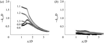
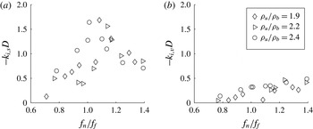
In order to more closely investigate the linear spatial amplification characteristics, the local spatial growth rates are directly compared to each other, again calculated using measured velocity profiles, this time plotted without using a logarithmic scale and the smoothing effects of the WKBJ integration. Figure 12 presents the axial dependence of the local spatial growth rates, calculated for several values of
 $f_{n}/f_{f}$
. The figure shows several noteworthy features. The first feature is that the sinuous spatial growth rate tends to exhibit a ‘bump’ near
 $x/D=1.5$
. The second feature is the sensitive, non-monotonic variation of the sinuous spatial growth rate as the value of
 $f_{n}/f_{f}$
changes. The third feature is the low-valued spatial growth rate of the varicose mode, and its relative insensitivity to the value of
 $f_{n}/f_{f}$
(over the studied range of this parameter). The details of these features are explored next.
Local spatial growth rates computed for the measured base flow, showing growth rates of oscillations at
 $f_{f}$
for the (a) sinuous and (b) varicose modes at
 ${\it\rho}_{u}/{\it\rho}_{b}=1.9$
for five
 $f_{n}/f_{f}$
values.

The bumps in the curves of
 $-k_{i,s}(x)D$
in figure 12(a) are resonant effects associated with the nearby weakly damped absolute instability mode. The absolute instability mode occurs at a saddle point in the complex
 ${\it\omega}(k)$
surface. As the real
 ${\it\omega}$
axis (i.e. the
 ${\it\omega}_{i}=0$
contour) passes near this saddle point, the associated value of
 $k_{i}$
is minimized, and as such the spatial growth rate,
 $-k_{i}$
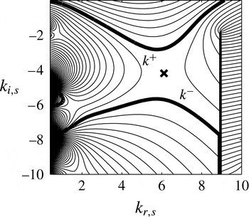
, is maximized. Figure 13 shows an example of this, by illustrating how the absolute instability mode’s saddle point draws the spatial stability analysis (the
 ${\it\omega}_{i}=0$
contour labeled as
 $k^{+}$
) to lower values of
 $k_{i}$
. The frequency of the absolute instability mode (which is nominally
 $f_{n}$
), and the topological location of its saddle point, are strong functions of
 $x/D$
and
 $f_{n}/f_{f}$
. Therefore, the resonant effect of the absolute instability mode is highly dependent on
 $x/D$
and
 $f_{n}/f_{f}$
and occurs when the forcing frequency, located on the real
 ${\it\omega}$
axis, is near where this axis crosses the topological ridge associated with the absolute instability mode’s saddle point. For the sinuous mode, this occurs close to
 $f_{n}/f_{f}=1$
at
 $x/D=1.5$
. For the varicose mode, this would occur at a frequency far from the studied range, such that the varicose mode is neither highly amplified nor highly sensitive to
 $f_{n}/f_{f}$
over the range of forcing frequencies studied.
Contour plot of complex
 ${\it\omega}_{i}(k)$
surface for the sinuous mode from local stability analysis of measured base flow for
 ${\it\rho}_{u}/{\it\rho}_{b}=1.9$
,
 $f_{n}/f_{f}=1.2$
and
 $x/D=1.3$
. At this axial position, the local flow is convectively unstable. Thick lines labeled
 $k^{+}$
and
 $k^{-}$
are contours of
 ${\it\omega}_{i}=0$
. The ‘
 $\boldsymbol{\times }$
’ marks the saddle point. Vertical thick line is a branch cut.

Figure 14 shows the dependence of the calculated linear spatial growth rate of the sinuous mode on the frequency ratio and density ratio at
 $x/D=1$
. The figure shows that the sinuous linear spatial growth rate peaks near
 $f_{n}/f_{f}=1$
, as expected. The fact that this peak occurs at a value of
 $f_{n}/f_{f}$
slightly greater than one is due to the fact that the local stability analysis predicts an absolute frequency slightly greater than the measured value of
 $f_{n}$
at this axial position. The figure also shows the influence of the density ratio, which does not have a clear influence over the range of density ratios studied here. Note that the influence of the density ratio on this forced spatial problem is substantially different than for the spatio-temporal problem, where the absolute growth rate of the sinuous mode is highly sensitive to the density ratio, such as shown in figure 1(b) (Emerson et al.
Reference Emerson, O’Connor, Juniper and Lieuwen2012; Yu & Monkewitz Reference Yu and Monkewitz1990). The reason for this is that the density ratio rescales the values of the iso-
 ${\it\omega}_{i}$
lines in figure 13, but has relatively little influence on their shapes.
Local spatial growth rates computed for the measured base flow versus
 $f_{n}/f_{f}$
, showing values for the (a) sinuous and (b) varicose modes at
 $x/D=1$
and
 $f=f_{f}$
.

(a,b) Distribution of energy at the forcing frequency between the sinuous and varicose modes, for (a)
 ${\it\rho}_{u}/{\it\rho}_{b}=2.4$
and (b)
 ${\it\rho}_{u}/{\it\rho}_{b}=1.9$
. Vertical axis represents fraction of the forced kinetic energy that is sinuous. (c,d) Varicose and sinuous forced response energies for (c)
 ${\it\rho}_{u}/{\it\rho}_{b}=2.4$
and (d)
 ${\it\rho}_{u}/{\it\rho}_{b}=1.9$
. Following a curve counter-clockwise (see arrows) from the origin corresponds to increasing
 $x/D$
. In (c,d), axial positions of
 $x/D=1$
are marked by circles, positions of
 $x/D=3$
are marked by squares, and positions of
 $x/D=5$
are marked by diamonds.

4.3. Interactions between sinuous and varicose flow disturbances: nonlinear effects
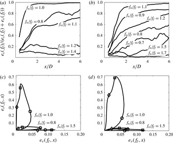
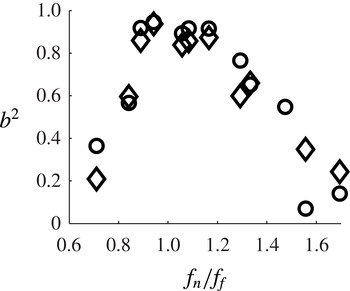
In order to better visualize the axial dependence of how energy is partitioned between sinuous and varicose modes, figure 15(a,b) plots the axial dependence of the fraction of the forced response energy that is in the sinuous mode,
 $e_{s}(f_{f})/[e_{s}(f_{f})+e_{v}(f_{f})]$
. Nominally, values greater than 0.5 indicate that the forced response is predominantly sinuous, and values less than 0.5 indicate that a varicose response dominates. The figure reinforces the observation from figure 10 that the varicose mode dominates the total forced disturbance energy near the bluff body. It also shows that the fraction of energy in the sinuous mode generally grows with downstream distance. Additionally, it demonstrates that the forced sinuous mode dominates in near-resonant cases, and that the varicose mode dominates in off-resonant cases. Comparing figure 15(a,b) shows a relative insensitivity of this varicose to sinuous disturbance mode phenomenon to density ratio, as expected based on the spatial growth rates shown in figure 14. Figure 15(c,d) provides an alternate view of these results by plotting the sinuous mode energy as a function of the varicose mode energy using axial position as a parameter. The curves begin at the origin and loop counter-clockwise as the axial position proceeds downstream. The figure shows that at resonance, the sinuous mode amplitude is augmented and the varicose mode amplitude is reduced. For the resonant cases in particular, the curves clearly show that the varicose and sinuous modes both grow initially, but that the varicose mode saturates and begins to decay while the sinuous mode continues to grow.
The growth of the sinuous mode relative to the varicose mode that occurs during resonant amplification manifests itself as vortex staggering. During longitudinal forcing, acoustic waves excite the two shear layers simultaneously, which roll up into larger structures that are symmetrically placed on the upper and lower half of the flow. These structures are initially symmetric, but stagger with downstream distance. This effect is evident in the iso-vorticity contours shown previously in the first column of figure 10. The degree and rate of staggering is a strong function of the forcing frequency. Although the density ratio is held constant, the vortical structures clearly evolve axially in very different manners depending on
 $f_{n}/f_{f}$
. In off-resonant cases, the vorticity iso-contours remain symmetrically configured to
 $x/D=5$
and beyond. For cases with strong resonant amplification, the vortices quickly stagger into a sinuous configuration.
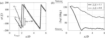
The spatial dependence of the staggering phenomenon can be quantified by defining a reference length scale where vortex staggering occurs. Of course, staggering does not occur at a discrete location, but instead the degree of flow response symmetry varies smoothly with axial position, as shown in figure 15. An independent approach to quantify the degree of staggering can be obtained by considering the phase difference between the unsteady vorticity for two spatial positions straddling the flow centreline, chosen here as
 $y/D=\pm 0.3$
. The axial variation of the vorticity phase at the forcing frequency is presented in figure 16(a). The nearly linear phase roll-off of each curve indicates a nearly constant phase speed of the vortical disturbances. Notice, however, that the phase difference,
 ${\rm\Delta}{\it\varphi}$
, is approximately
 $180^{\circ }$
near the bluff body, and decreases to almost zero farther downstream. The phase difference between these two lines is shown in figure 16(b) at two frequency ratios. Based on this vorticity phase difference, a characteristic stagger length,
 $L_{stagger}$
, is defined as the axial location where
 ${\rm\Delta}{\it\varphi}=90^{\circ }$
(illustrated in figure 16
a).
(a) Axial dependence of the phase of the vorticity from the upper and lower side of the flow centreline. The phase is extracted from the Fourier coefficient at the forcing frequency. Flow conditions are
 ${\it\rho}_{u}/{\it\rho}_{b}=1.9$
, and
 $f_{n}/f_{f}=1.1$
. (b) Vorticity phase difference, across the flow centreline, for two values of
 $f_{n}/f_{f}$
at
 ${\it\rho}_{u}/{\it\rho}_{b}=1.9$
.

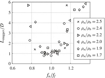
Figure 17 plots the dependence of the stagger length,
 $L_{stagger}$
, upon
 $f_{n}/f_{f}$
for a number of density ratios. Note that
 $L_{stagger}$
is dramatically reduced when
 $f_{n}\approx f_{f}$
. Similar to the growth rate discussion,
 ${\it\rho}_{u}/{\it\rho}_{b}$
does not have a discernible influence on
 $L_{stagger}$
. Staggering is observed at density ratios as high as 2.5, where the flow is globally stable (see figure 6), and has a weakly damped global mode.
Stagger length as a function of
 $f_{n}/f_{f}$
for all density ratios.

The first harmonic of the forcing frequency appears in both the varicose and sinuous modes and was noted earlier in the context of figures 10 and 11. The behaviour of the harmonics is discussed further in appendix B, which argues that resonant amplification involves a nonlinear interaction between the forced varicose mode and the forced sinuous mode, and that the first harmonic of the varicose mode is integral to this nonlinear interaction. This nonlinear relationship is likely due to the fact that the varicose mode sheds vortical structures from the bluff body once per cycle of the mode, while in contrast the sinuous mode sheds vortical structures from the bluff body at a rate that is twice the mode’s frequency (i.e. it sheds structures from both sides of the bluff body, alternately, in one cycle). Therefore, the varicose mode must operate at twice the frequency of the sinuous mode for these shedding events to be temporally aligned. This concept has been explored previously by (Leontini, Jacono & Thompson Reference Leontini, Jacono and Thompson2013), who showed that the sinuous mode is highly receptive to longitudinal excitation at twice its global mode frequency. Interestingly, this work suggests that forcing at
 $2f_{n}$
could directly excite the sinuous mode, without depending on a coupling to the varicose mode.
To summarize this section, resonant amplification appears to occur due to the following series of processes. First, the symmetric forcing excites the varicose mode in the separating shear layers of the bluff body. Simultaneously, small unavoidable asymmetries in the flow and the geometry allow the forcing to excite the sinuous mode. Initially, these modes are independently linearly amplified, as suggested by figure 17(a). When
 $f_{n}/f_{f}\approx 1$
, the sinuous mode is preferentially linearly amplified relative to the varicose mode, near
 $x/D=1.5$
. As the sinuous mode grows, it begins to nonlinearly interact with the varicose mode, extracting energy from it via the varicose mode’s first harmonic. Through this nonlinear interaction, the growth of the sinuous mode is boosted beyond its linear growth, and it becomes the dominant fluid dynamic mode.
Axial dependence of spectra of the forced sinuous and varicose responses, for (a,c) flow and (b,d) flame. Conditions are
 ${\it\rho}_{u}/{\it\rho}_{b}=1.9$
. (a,b)
 $f_{n}/f_{f}=1.1$
and (c,d)
 $f_{n}/f_{f}=1.3$
.

5. Forced flame response dynamics
5.1. Forced flame response structure
This section focuses on the flame response at the forcing frequency,
 $f=f_{f}$
. Understanding the ultimate relationship between the ‘input’ acoustic forcing and the ‘output’ heat release fluctuations is the key remaining question in the combustion instability problem. To begin, figure 18 plots flame response spectra, decomposed into sinuous and varicose disturbances, as functions of axial position. The figure shows these spectra for the flame dynamics at two values of
 $f_{n}/f_{f}$
, and compares them to spectra of the flow dynamics at the same conditions. This comparison illustrates the fact that the local flame and flow dynamics, although related, are not the same. The flame wrinkling at any given spatial location is a convolution integral of the time-delayed disturbance field at all upstream locations. For example, (5.1) shows a solution of the linearized G-equation for a single valued anchored flame front reproduced from equation (11.43) in Lieuwen (Reference Lieuwen2012), that relates the local flame position and velocity field, clearly illustrating this non-local relationship:
 $$\begin{eqnarray}L^{\prime }(y_{s},t_{s})=\frac{1}{u_{t,0}^{u}\sin {\it\theta}}\int _{0}^{y_{s}}\frac{1}{\sin {\it\theta}}v_{F,n}^{\prime }\left\{s,t_{s}-\frac{y_{s}-s}{u_{t,0}^{u}\sin {\it\theta}}\right\}\,\text{d}s.\end{eqnarray}$$
In (5.1),
 $u_{t,0}^{u}$
represents the local time-averaged unburned velocity tangent to the flame front,
 $v_{F,n}^{\prime }$
is the forced local velocity oscillation normal to the flame front and the convolution integral is performed across the transverse coordinate,
 $y_{s}$
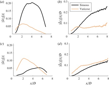
. Thus, the local flame behaviour reflects not only the local flow dynamics, but also the dynamics from all upstream positions along the flame (Boyer & Quinard Reference Boyer and Quinard1990). For example, figure 18(a,c) reveals that the varicose mode of the flow fluctuations is significantly weaker than the sinuous mode at
 $x/D=6$
. However, the flame spectra (b,d) show that a strong varicose component remains at
 $x/D=6$
, which the flame ‘remembers’ because the strong varicose flow structure farther upstream excite symmetric flame wrinkles which subsequently convect downstream. Therefore, the strongly sinuous structure of the forcing flow field is not completely mirrored in the flame response – rather, the flame exhibits significant varicose oscillations as well, even at spatial locations where the varicose disturbance field is negligible and completely dominated by sinuous disturbances. However, sinuous and varicose features on the flame exhibit completely different heat release response characteristics, a topic that is emphasized in the rest of this section. Despite this fact, resonant amplification can still significantly alter the forced response structure of the flame.
5.2. Local flame heat release response
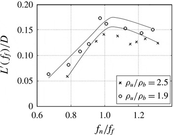
This section considers the forced response magnitude of the flame position displacement and the axial distribution of heat release rate fluctuations, and their sensitivities to frequency ratio and density ratio. As would be expected, resonant forcing manifests itself in large fluctuations in flame edge displacement. For example, figure 19 plots the dependence of the forced response magnitude of flame wrinkling amplitude upon forcing frequency, showing that it peaks near
 $f_{n}=f_{f}$
.
Flame edge displacement amplitude at
 $x/D=3$
as a function of
 $f_{n}/f_{f}$
.

The local heat release rate of the flame is proportional to the flame area. The flame position fluctuations directly cause unsteady flame area perturbations,
 $S$
, according to the relationship:
 $\text{d}S\approx \sqrt{1+(\text{d}L/\text{d}x)^{2}}\,\text{d}x$
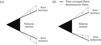
. Therefore, for a given flame branch, the magnitude of flame flapping is roughly proportional to the local heat release rate fluctuations. However, the heat release rate fluctuations at each axial location are controlled by the relative phasing of the upper and lower flame branches. As such, the degree of symmetry of the two branches has an important impact on the relationship between local flame flapping and the associated heat release fluctuations. In particular, varicose flow/flame oscillations cause the heat release oscillations of the two flame branches to be in phase, while sinuous oscillations cause phase-cancellation of flame surface area between the two flame branches. To visualize this, figure 20 illustrates differential lengths of flames perturbed by varicose and sinuous structures. The figure demonstrates how the sinuous structure elongates one flame branch while shortening the other. Thus, in terms of heat release oscillations, resonant amplification leads to two competing phenomena: large flame displacement and surface area fluctuations of the individual flame branches, but a sinuous flame structure. This is illustrated with the following sum of the heat release rate of the two flame branches:
 $$\begin{eqnarray}q(x,f)=q_{+}(x,f)+q_{-}(x,f).\end{eqnarray}$$
The heat release rate of one flame branch may be related to the heat release rate of the other by a phase offset,
 ${\it\theta}$
, such that
 $q_{-}(x,f)=q_{+}(x,f)\text{cos}({\it\theta}(x,f))$
. Equation (5.2) then reduces to the following expression:
 $$\begin{eqnarray}q(x,f)=\underbrace{q_{+}(x,f)}_{\begin{array}{@{}c@{}}wrinkling\\ amplitude\\ effect\end{array}}\underbrace{\cos ^{2}\left\{\frac{{\it\theta}(x,f)}{2}\right\}}_{\begin{array}{@{}c@{}}stagger\\ effect\end{array}}.\end{eqnarray}$$
This expression illustrates the competing effects of flame edge displacement and staggering. Flame edge displacement drives the unsteady heat release rate of a given branch, and staggering affects the phase offset between the two branches. Note that a phase offset of
 ${\it\theta}=180^{\circ }$
drives this expression to zero, even if the local heat release of the individual flame branches is large.
Notional sketch of a differential length of flame, perturbed by (a) varicose structure and (b) sinuous structure. Flame area change, relative to the mean, is visualized by comparing dashed lines to solid lines.

The phase difference between the upper and lower flame branches at the forcing frequency is denoted by
 ${\rm\Delta}{\it\varphi}=\angle \hat{L}_{upper}(f_{f})-\angle \hat{L}_{lower}(f_{f})$
. The flame is sinuous when
 ${\rm\Delta}{\it\varphi}=0^{\circ }$
, since the upper and lower branches are moving ‘up’ in synchronization. It is important to notice that this sinuous configuration,
 ${\rm\Delta}{\it\varphi}=0^{\circ }$
, occurs when the heat release of the two flame branches is out of phase,
 ${\it\theta}=180^{\circ }$
.
The local chemiluminescence amplitude,
 $q^{\prime }(x,f)$
, is quantified as the Fourier transformed unsteady luminosity from the chemiluminescence images, and is non-dimensionalized by the time-averaged chemiluminescence,
 $Q_{0}(x)$
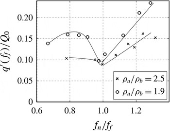
. Relating heat release oscillations to chemiluminescence fluctuations is known to be a good approximation in cases where the fuel/air ratio of the approach flow is constant (Gaydon & Wolfhard Reference Gaydon and Wolfhard1970; Lee & Santavicca Reference Lee and Santavicca2003). The dependence of the local heat release fluctuations,
 $q^{\prime }(x,f)$
, on
 $f_{n}/f_{f}$
is plotted in figure 21, at a fixed axial location. This figure shows that the local heat release oscillations decrease when the forcing frequency is close to the global mode frequency, an effect that is more pronounced at lower density ratios.
Local heat release amplitude at
 $x/D=3$
versus
 $f_{n}/f_{f}$
.

This local minimum in heat release reflects the fact that the phase cancellation effect dominates the increased flame displacement effect when
 $f_{n}\approx f_{f}$
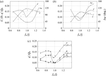
. To better visualize these competing effects, figure 22(a,b) overlay the frequency dependence of the flame displacement amplitude, the degree of stagger between the two flame branches (
 ${\rm\Delta}{\it\varphi}$
) and the local heat release amplitude. Notice that the flame displacement amplitude is maximized when
 $f_{n}\approx f_{f}$
. However, when
 $f_{n}\approx f_{f}$
, the phase difference between the two flame branches is close to a sinuous configuration (the phase is about
 $45^{\circ }$
; the reason that it is not
 $0^{\circ }$
is due to the flame ‘memory effect’ discussed above), and the local heat release amplitude is minimized. Figure 22(c) shows the axial dependence of the relationship of local heat release amplitude to frequency ratio. As the figure suggests, the minimum in local heat release amplitude when
 $f_{n}\approx f_{f}$
persists at all axial positions downstream of the initial staggering. Thus, the local heat release response of low density ratio flames under resonant forcing conditions is less than that of flames forced off-resonance.
Frequency dependence of flame edge displacement amplitude, local heat release amplitude and flame stagger at
 $x/D=3$
, (a)
 ${\it\rho}_{u}/{\it\rho}_{b}=1.9$
and (b)
 ${\it\rho}_{u}/{\it\rho}_{b}=2.5$
. (c) Dependence of local heat release amplitude on frequency at three axial positions for
 ${\it\rho}_{u}/{\it\rho}_{b}=1.9$
.

Spatially integrated, forced heat release rate amplitude versus flame length for (a)
 ${\it\rho}_{u}/{\it\rho}_{b}=2.5$
and (b)
 ${\it\rho}_{u}/{\it\rho}_{b}=1.9$
.

This phase cancellation effect has important and very non-intuitive implications for the motivating phenomenon of combustion instability. It shows that, for longitudinal acoustic modes, alignment of the hydrodynamic global mode frequency with the acoustic excitation frequency inhibits the flame’s forced heat release response due to the flame’s resulting sinuous response structure. Thus, for low density ratio flames, a situation where the frequency of the hydrodynamic global mode overlaps a longitudinal acoustic mode frequency is not such a dangerous situation as previously thought (Schadow & Gutmark Reference Schadow and Gutmark1992).
5.3. Global heat release response
The response of the spatially integrated heat release, referred to here as the global heat release, is of particular interest from a combustion instability standpoint. The global heat release is defined as
 $$\begin{eqnarray}Q(L_{f},t)=\int _{x=0}^{x=L_{f}}q(x,t)\,\text{d}x,\end{eqnarray}$$
where
 $L_{f}$
is the axial flame length. The global heat release is a strong function of
 $L_{f}$
, due to axial phase variation in the local heat release. Figure 23 plots the global heat release magnitude at the forcing frequency as a function of axial integration length. In order to understand these behaviours, note that the flame wrinkle wavelength,
 ${\it\lambda}_{f}$
, is related to the flame wrinkle propagation speed and frequency according to
 ${\it\lambda}_{f}=u_{f}/f$
, where
 $u_{f}$
is a reference flame wrinkle propagation speed. Equation (5.4) is rewritten to consider only the component of the local heat release at the forcing frequency:
 $$\begin{eqnarray}\hat{Q}(L_{f},f)=\int _{x=0}^{x=L_{f}}|\hat{q}(x,f)|\text{exp}\left\{\text{i}\left(\frac{2{\rm\pi}}{{\it\lambda}_{f}}x\right)+\text{i}{\it\theta}\right\}\text{d}x.\end{eqnarray}$$
The normalizing reference length scale,
 ${\it\lambda}_{f}$
is determined experimentally from the spatial evolution of the Fourier coefficients of the flame edge displacement according to (5.6), and represents an axially-averaged quantity from the domain
 $2<x/D<14$
.
 $$\begin{eqnarray}{\it\lambda}_{f}=2{\rm\pi}\frac{{\rm\Delta}x}{{\rm\Delta}\angle \hat{L}}.\end{eqnarray}$$
Equation (5.5) shows that the global heat release is an oscillatory function of the flame length. In fact, if the local heat release magnitude was a constant function of axial position, i.e.
 $|q(x,f_{f})|=|q(f_{f})|$
, then the global heat release would have a perfect pattern of nodes and antinodes spaced at integer multiples of
 ${\it\lambda}_{f}$
,
 $|\hat{Q}(L_{f},f_{f})|=|\text{sin}({\rm\pi}L_{f}/{\it\lambda}_{f}(f))|$
. Such a pattern is easily recognized in the data shown in figure 23, which shows the global heat release magnitude at the forcing frequency as a function of flame length (integration length).
The nodes and antinodes in this pattern arise due to destructive/constructive phase interference between the highs and lows on the instantaneous local heat release wave,
 $q^{\prime }(x)$
. Figure 23 shows the globally integrated forced heat release rate amplitude as a function of flame length for two density ratios and two values of
 $f_{n}/f_{f}$
. The figure shows that during resonant forcing (
 $f_{n}/f_{f}=1.0$
) there is a slight reduction in global heat release response for most flame lengths compared to
 $f_{n}/f_{f}=0.8$
. The effect is not as pronounced as it is for the local heat release response (see figure 22
c) since the varicose portion of the flame structure at upstream axial positions is included in the spatially-averaged heat release. Interestingly, the global heat release response of the flame shows sensitivity to the density ratio. As shown in the previous sections, the flow symmetry (namely, the transition from varicose to sinuous structure) is insensitive to the density ratio over the range of density ratios studied. However, the overall amplitude of the sinuous mode is slightly higher at lower density ratios. This is evidenced at resonant conditions by comparing figure 15(c,d). The convolution integral, (5.1), that describes the local flame response integrates this into a more noticeable effect, which can be seen by comparing the
 $L^{\prime }/D$
values between figure 22(a,b). This effect is further integrated by (5.5) to non-negligible proportions in the global heat release response (see figure 23
a,b). Thus, the role of the density ratio is to slightly increase the amplitude of the sinuous mode, to noticeably increase the magnitude of local flame flapping during resonance and to significantly increase the global heat release response of the flame. A brief investigation of higher density ratios, where the sinuous global mode is heavily damped, suggests that no level of forcing amplitude or alignment of
 $f_{n}$
and
 $f_{f}$
results in resonant amplification. Not surprisingly,
 $f_{n}/f_{f}$
has little effect on the global heat release in this case.
In summary, the global heat release is a strong function of the integration length (the flame length). At some flame lengths, global heat release response amplitude is very small while at others it is significant (as much as 10 % of the time-averaged heat release rate). For flame lengths associated with significant global heat release, the global heat release response magnitude is slightly minimized when the forcing frequency equals the natural asymmetric vortex shedding frequency, and when the density ratio is lowered only enough for the forced shedding to stagger to an asymmetric pattern. An important observation is that alignment of the forcing and hydrodynamic global mode frequencies does not cause a maximum in global heat release response and therefore does not promote combustion instability. This conclusion is valid only for longitudinal acoustic modes and is likely to differ for transverse acoustic modes.
6. Conclusions
This paper addresses the thermoacoustic instability problem in bluff body combustors. Specifically, it focuses on the longitudinally acoustically excited fluid dynamics and the resulting influence on the unsteady heat release of combustion. The experimental study shows that when the forcing frequency is in the vicinity of the global mode frequency, resonant amplification occurs. During resonant amplification, the wake, and hence the flame, respond more strongly at the forcing frequency than the global mode frequency. When this happens, the vortices which initially roll up in a varicose configuration (due to the symmetric nature of the forcing) quickly stagger to a sinuous pattern. This is triggered by the high spatial growth rate of the sinuous mode at resonant conditions followed by a nonlinear coupling between the sinuous and varicose modes.
The vortical flow field wrinkles the flame sheets, which similarly exhibit forced sinuous oscillations during resonant amplification. This is associated with an increase in the oscillatory flame edge displacement, but a decrease in local oscillatory heat release fluctuations at the forcing frequency. This effect is also present, although less pronounced, in the spatially integrated heat release response. This is important and non-intuitive, as it shows that forcing a bluff body combustor at its hydrodynamic global mode frequency actually leads to a slight reduction in the flame’s heat release response. Finally, this analysis shows that the global heat release response is a strong function of flame length, exhibiting a pattern of nodes and antinodes. For flame lengths associated with significant global heat release response, this response is minimized when the density ratio is just low enough (but no lower) for vortex staggering to occur, and when the acoustic and hydrodynamic frequencies are equal.
Several future studies are motivated by this work. First, future work should also consider transverse forcing of a related configuration. From the fluid mechanic perspective, the forcing would more directly excite the sinuous disturbance mode and the energy transfer between sinuous and varicose disturbances would be less dynamically significant. From the thermoacoustic instability perspective, an additional degree of freedom would be present if a pressure node were to exist at the bluff body centreline, leading to a
 $180^{\circ }$
phase offset of the pressure oscillations at the two flame branches. In this case, even if the heat release oscillations from the two flame branches excited by sinuous flow disturbances were out of phase, they could each add (or remove) energy to the acoustic field, as described by the Rayleigh criterion, and thus not cancel each other’s contribution to the acoustic energy in the system.
Another important point from this study is the strong difference between the effect of density ratio upon the forced response relative to its nominal spatio-temporal dynamics, namely its strong influence upon the global stability of the flow but its weak impact on the forced response of a globally stable flow. As discussed in § 1, a number of studies have noted the importance of density stratification on the spatio-temporal dynamics of other canonical flows such as jets and backward facing steps. Similar future work on their forced response characteristics would be useful for further generalizing the results of this work on density stratification influences on forced shear flows.
Appendix A. Effect of forcing on the time-averaged flow
This appendix summarizes the forced response characteristics of the time-averaged flow. Consistent with prior observations in non-reacting wakes (Cardell Reference Cardell1993), reacting wakes (Shanbhogue Reference Shanbhogue2008) and cavities (Abdelkhalek, Ghoneim & Ghoniem Reference Abdelkhalek, Ghoneim and Ghoniem2001), forcing leads to a reduction in recirculation zone length. The recirculation zone length,
 $L_{r}$
, is defined as the distance from the bluff body trailing plane to the centreline axial velocity stagnation point (see figure 24
a). Figure 24(b) plots recirculation zone length as a function of lip velocity and density ratio. In general, the figure shows that low lip velocities and the presence of forcing lead to reduced recirculation zone lengths. The density ratio weakly influences
 $L_{r}$
, which generally increases with increasing density ratio (Emerson et al.
Reference Emerson, O’Connor, Juniper and Lieuwen2012).
(a) Streamlines for
 ${\it\rho}_{u}/{\it\rho}_{b}$
,
 $U_{lip}=50~\text{m}~\text{s}^{-1}$
, for top half: unforced flow, and bottom half: forced flow. (b) Shows comparison of forced to unforced recirculation zone lengths. Filled symbols indicate forced flows, unfilled symbols indicate unforced flows.

Phase portraits of the varicose mode energy plotted as a function of the sinuous mode energy at
 ${\it\rho}_{u}/{\it\rho}_{b}=2.4$
, for a wake at (a)
 $f_{n}/f_{f}=1.3$
,
 $x/D=3$
, with weak resonant amplification, (b)
 $f_{n}/f_{f}=1.0$
,
 $x/D=1$
, with strong resonant amplification, (c)
 $f_{n}/f_{f}=1.3$
,
 $x/D=3$
, with weak resonant amplification, (d)
 $f_{n}/f_{f}=1.0$
,
 $x/D=3$
, with strong resonant amplificaiton.

Appendix B. Harmonics of the forcing frequency
The first harmonic of the forcing frequency appears in both the varicose and sinuous modes. With resonant forcing, the varicose mode disturbances have similar amplitudes at
 $f/f_{f}=1$
and 2, while the harmonic of the sinuous mode is orders of magnitude less than the response at the forcing frequency. Of course, one would expect that nonlinearities would lead to the appearance of harmonics, particularly at conditions where the system response at the forcing frequency is strongest. As shown in figure 25(b), the amplitude of the harmonic of the sinuous mode does monotonically increase with the amplitude at the forcing frequency. For reference, a quadratic nonlinearity would lead to a relationship of the form
 $e_{s}(2f_{f})\propto [e_{s}(f_{f})]^{2}$
, which is shown as a reference line in figure 25(a,b). However, the varicose mode harmonic exhibits opposite behaviour. Figure 25(a) shows that the response of the varicose mode at
 $f=f_{f}$
and
 $f=2f_{f}$
are weakest and strongest during resonant amplification, respectively. Repeating a point made earlier, at resonance the amplitude of the sinuous mode increases and the amplitude of the varicose mode decreases at the forcing frequency, while the harmonic of the varicose mode increases. In other words, the growth of the sinuous mode is at the expense of the varicose mode, which emphasizes the strong role of nonlinearity in its growth. The physical mechanism for this energy transfer appears to be staggering of the initially symmetric vortices, as discussed in the main text.
The response of the varicose mode at
 $f=2f_{f}$
is due to a nonlinear coupling between the fundamental varicose and sinuous responses during resonant amplification. This can be seen from the cross-bicoherence,
 $b^{2}(f_{1},f_{2})$
, between the sinuous mode at
 $f_{1}=f_{f}$
and the varicose mode at
 $f_{2}=f_{f}$
. The cross-bispectrum is a generalization of the cross-coherence function, and quantifies the coherence between functions at different frequencies; in particular, its structure focuses on quadratic nonlinear relationships. Higher order moment spectra can similarly be used to quantify higher order nonlinear input-output relationships (Nikias & Petropulu Reference Nikias and Petropulu1993). Testing for nonlinear quadratic relationships requires a third signal, which could be either the sinuous or the varicose mode, and which must be sampled in the frequency domain at
 $f_{3}=f_{1}+f_{2}=2f_{f}$
. For example, using the varicose mode at
 $2f_{f}$
for this third signal, leads to the following cross-bicoherence,
 $b^{2}$
(Swami, Mendel & Nikias Reference Swami, Mendel and Nikias1993).
 $$\begin{eqnarray}b^{2}(f_{f},f_{f})=\frac{\left\{\displaystyle \frac{1}{N}\mathop{\sum }_{n=1}^{N}\hat{v}_{s}(f_{f})\hat{v}_{v}(f_{f})\hat{v}_{v}^{\ast }(2f_{f})\right\}^{2}}{\left\{\displaystyle \frac{1}{N}\mathop{\sum }_{n=1}^{N}\hat{v}_{s}(f_{f})\hat{v}_{s}^{\ast }(f_{f})\right\}\left\{\displaystyle \frac{1}{N}\mathop{\sum }_{n=1}^{N}\hat{v}_{v}(f_{f})\hat{v}_{v}^{\ast }(f_{f})\right\}\left\{\displaystyle \frac{1}{N}\mathop{\sum }_{n=1}^{N}\hat{v}_{v}(2f_{f})\hat{v}_{v}^{\ast }(2f_{f})\right\}},\end{eqnarray}$$
where the asterisk symbolizes a complex conjugate.
The diamonds in figure 26 present the cross-bicoherence for the sinuous and varicose modes at the forcing frequency, coupled with the varicose mode at the first harmonic of the forcing frequency. The figure shows a local maximum at
 $f_{n}=f_{f}$
, with values of nearly
 $b^{2}=1$
. This suggests that a phase-coupled, quadratic nonlinearity is present during resonant amplification. More specifically, it demonstrates phase-coupling between the varicose oscillations at
 $f_{f}$
, the sinuous oscillations at
 $f_{f}$
and the varicose oscillations at
 $2f_{f}$
. This supports our hypothesis that resonant amplification involves a nonlinear interaction between the forced varicose mode and the forced sinuous mode, and that the first harmonic of the varicose mode is integral to this nonlinear interaction.
Cross-bicoherence between the varicose mode at
 $f_{f}$
and the sinuous mode at
 $f_{f}$
, through the varicose mode at
 $2f_{f}$
(diamonds) and through the sinuous mode at
 $2f_{f}$
(circles). Conditions are
 ${\it\rho}_{u}/{\it\rho}_{b}=1.9$
,
 $x/D=3$
.

The circles overlaid in figure 26 show a similar trend, when the cross-bicoherence is calculated using the harmonic of the sinuous mode,
 $\hat{v}_{s}(2f_{f})$
, rather than the harmonic of the varicose mode,
 $\hat{v}_{v}(2f_{f})$
. This result is somewhat expected, since the harmonic of the sinuous mode is presumably born from nonlinearity associated with the fundamental sinuous mode (see discussion around figure 25
b), and as such should be phase-coupled to the fundamental sinuous oscillations. Therefore, the authors hypothesize that the strong harmonic of the varicose response (and the strong cross-bicoherence with harmonic varicose coupling) is generated during the phase-coupling between the sinuous and varicose oscillations, while the harmonic of the sinuous mode (and the strong cross-bicoherence with harmonic sinuous coupling) is simply due to nonlinearity of the sinuous mode with itself. Nonetheless, correlation does not imply causality. A rigorous assessment of this question will require a nonlinear analysis of the coupling between sinuous and varicose modes.