1. Introduction
Turbulence effectively mixes fluids through a multiscale process (Danckwerts Reference Danckwerts1952, Reference Danckwerts1958; Dimotakis Reference Dimotakis2005): fluids are entrained at the largest scales, dispersed by eddies of varying sizes until the length and time scales are sufficiently small for viscous, heat and mass diffusion to act. Dimotakis (Reference Dimotakis2005) suggests that turbulent mixing can be categorized into three ‘levels’. Extensive research has been dedicated to understanding mixing of passive scalars (level 1), which is decoupled from the fluid dynamics (Warhaft Reference Warhaft2000; Sawford Reference Sawford2001), specifically in the context of dispersion of collections of small particles in turbulent flows, e.g. pollutants, smoke or, under certain circumstances, clouds. At the other end of the spectrum, level 3 mixing is characterised by a strong coupling between the fluid dynamics and the composition of the fluids, such as in combustion processes. A variety of problems in atmospheric, oceanic and astrophysical flows lie in between, where the mixing is coupled to the dynamics (level 2 mixing), e.g. through variations in density and composition, but with little modification to the fluids themselves. A considerable amount of research in level 2 mixing, the focus of this work, is concerned with hydrodynamic instabilities at interfaces (Chandrasekhar Reference Chandrasekhar1961; Sharp Reference Sharp1984; Rogers & Moser Reference Rogers and Moser1992; Brouillette Reference Brouillette2002) driven by continuous and impulsive acceleration fields (Rayleigh–Taylor and Richtmyer–Meshkov) and shear (Kelvin–Helmholtz), which may ultimately evolve to turbulence. At the present time, there is no consensus as to whether the resulting turbulence can be described by Kolmogorov–Obukhov ideas (Soulard & Griffond Reference Soulard and Griffond2012) or not (Poujade Reference Poujade2006; Abarzhi Reference Abarzhi2010). The lack of understanding of turbulent mixing has impeded progress in a variety of problems, e.g. understanding how heavy and light elements mix after the collapse of a supernova (Kifonidis et al. Reference Kifonidis, Plewa, Scheck, Janka and Muller2006) and the inability to achieve ignition in inertial confinement fusion (Lindl Reference Lindl1995; Thomas & Kares Reference Thomas and Kares2012).
One of the main difficulties in level 2 mixing lies in the realisation that the turbulence is not isotropic at all scales, thus preventing direct application of classical Kolmogorov–Obukhov–Corrsin (KOC) theory (Kolmogorov Reference Kolmogorov1941; Obukhov Reference Obukhov1949; Corrsin Reference Corrsin1951). From a pragmatic viewpoint, the Rayleigh–Taylor instability is a useful illustration of anisotropy in turbulence (Cabot & Cook Reference Cabot and Cook2006; Abarzhi Reference Abarzhi2010). Large-scale features such as density variations and an acceleration field (e.g. body force, rotation) introduce an asymmetry, thus leading to anisotropy. The misalignment of the (hydrostatic) pressure and density gradients at unstably stratified interfaces generates baroclinic vorticity that feeds the instability, thus ultimately leading to fully mixed turbulence through a multistage process (Cook & Dimotakis Reference Cook and Dimotakis2001; Cabot & Cook Reference Cabot and Cook2006). Anisotropy is observed at the integral and Taylor scales in Rayleigh–Taylor turbulence, although the dynamics at the Kolmogorov microscale remain isotropic (Cabot & Zhou Reference Cabot and Zhou2013). In these problems, the occurrence of anisotropy is attributable to both the presence of a large-scale density gradient across the mixing region and of an acceleration field. In particular, the relative alignment and magnitude of these vectors determines the stability of the Rayleigh–Taylor set-up and the amount of baroclinic vorticity generation. The acceleration field acts as a directional force term scaled by local density differences, and allows the flow to sustain anisotropy (Cook & Dimotakis Reference Cook and Dimotakis2001; Ristorcelli & Clark Reference Ristorcelli and Clark2004; Livescu & Ristorcelli Reference Livescu and Ristorcelli2007). More specifically, in stably stratified turbulence, mixing due to the dispersion of light and heavy fluids by turbulence in the direction of gravity requires work to be done against buoyancy forces, which reduce the motions in this direction and thus lead to anisotropy (Turner Reference Turner1968; Linden Reference Linden1980). In Rayleigh–Taylor turbulence, an acceleration field and a density gradient are always both present; it is thus not possible to identify the individual contribution of each one to anisotropy. In cases when there is a gradient in composition as well, viscosities may be different in the two fluids, leading to a different turbulent kinetic energy dissipation rate. In addition, species diffusion in miscible fluids tends to locally smoothen the density gradient and consequently reduce the local rate of baroclinic vorticity production (
 ${\sim}\boldsymbol{{\rm\nabla}}{\it\rho}\times \boldsymbol{{\rm\nabla}}p$
), compared with the immiscible counterpart. Thus, the dynamics in Rayleigh–Taylor turbulence are directly affected by the mixing process, by contrast to passive scalar (level 1) mixing. In addition, the kinematic viscosities in each fluid may be different, such that the turbulence decays at different rates in each region, another source of anisotropy (Tordella & Iovieno Reference Tordella and Iovieno2011). Furthermore, non-Boussinesq effects become important at high Atwood numbers. Livescu & Ristorcelli (Reference Livescu and Ristorcelli2007) studied turbulent mixing between two incompressible miscible fluids in an unstably stratified medium. The mean pressure evolves dynamically, as mixing occurs between the light and heavy fluids, leading to non-Boussinesq effects. In particular, Livescu & Ristorcelli (Reference Livescu and Ristorcelli2008) and Livescu et al. (Reference Livescu, Ristorcelli, Petersen and Gore2010) state that the pure light fluid mixes faster than the pure heavy fluid, resulting in an asymmetric mixing process. These difficulties present challenges for investigating anisotropy in turbulent mixing through the Rayleigh–Taylor instability.
As our first step toward a better understanding of level 2 mixing in general and Rayleigh–Taylor turbulence in particular, we seek to isolate the effect of a density gradient from that of gravity on the turbulence. In contrast to past studies of Rayleigh–Taylor mixing, we start by neglecting gravity to consider passive scalar mixing, and subsequently superpose a density gradient on an initial isotropic field. Statistics of passive scalar mixing are known from numerical and experimental freely decaying (grid) turbulence studies (Warhaft Reference Warhaft2000; Sawford Reference Sawford2001). In one such set of wind tunnel experiments, Jayesh, Tong & Warhaft (Reference Tong and Warhaft1994) and Tong & Warhaft (Reference Tong and Warhaft1994) used a conventional grid to generate an initial turbulent field with
 $30\leqslant \mathit{Re}_{{\it\lambda}}\leqslant 130$
, where
 $\mathit{Re}_{{\it\lambda}}$
is the initial Taylor-scale Reynolds number, and imposed a linear mean cross-stream temperature gradient upstream of the grid. Due to the relatively low Mach number (
 $M\approx 0.017$
) and negligible buoyancy effects over the time scales of interest, temperature can be assumed to behave as a passive scalar in those experiments in which the Schmidt number is 0.7. The scalar spectra in the inertial range approached the expected
 $-5/3$
slope sooner than those of velocity, and the dissipation of scalar variance was found to be 20 % larger in the direction of the temperature gradient. Mydlarski & Warhaft (Reference Mydlarski and Warhaft1998) investigated higher
 $\mathit{Re}_{{\it\lambda}}$
(up to 700) by employing an active grid technique to generate the initial turbulent field. Other passive scalar studies in grid turbulence focused on dispersion of a thermal wake behind a heated wire (Anand & Pope Reference Anand and Pope1983; Warhaft Reference Warhaft1984; Stapountzis et al.
Reference Stapountzis, Sawford, Hunt and Britter1986), in which case the mean temperature profile was found to be Gaussian, while the variance was not. The mean thermal wake development was shown to consist of three stages: molecular diffusive (
 $h\sim t^{1/2}$
), turbulent convective (
 $h\sim t$
) and turbulent diffusive
 $(h\sim t^{1-n/2})$
, where
 $h$
is the mixing region width and
 $n$
is the time exponent of the kinetic energy decay rate. However, the tunnel was not sufficiently long to reach the expected growth in the final stage. In the context of stably stratified turbulence, Huq & Britter (Reference Huq and Britter1995a
) studied the role of Schmidt number on passive scalar mixing between two layers of different fluids due to grid-generated turbulence in water tunnel experiments. The scalar Taylor microscales were found to be dependent on the Schmidt number, whereas integral scales were not. Huq & Britter (Reference Huq and Britter1995b
) also investigated the evolution of a mixing region starting from an initially sharp interface between two fluids of different densities. The mixing region grew initially due to turbulent diffusion, similar to the passive case, but at later times decreased because of buoyancy effects.
In the Richtmyer–Meshkov instability with reshock, a variable-density turbulent mixing region may develop (Hill, Pantano & Pullin Reference Hill, Pantano and Pullin2006; Thornber et al. Reference Thornber, Drikakis, Youngs and Williams2011; Tritschler et al. Reference Tritschler, Olson, Lele, Hickel, Hu and Adams2014). While the mixing region grows due to turbulence diffusion, the turbulence decays since no further energy feeds it (Drake Reference Drake2006). In another related study, Lamriben, Cortet & Moisy (Reference Lamriben, Cortet and Moisy2011) investigated the role of background rotation on freely decaying turbulence in a water-filled rotating tank. By measuring the anisotropic energy flux density and the energy distribution at different scales, Lamriben et al. (Reference Lamriben, Cortet and Moisy2011) observed in their experiments that anisotropy caused by rotation (i.e. Coriolis force) appears to result in small-scale anisotropy. This result lies in contrast with anisotropy observed in Rayleigh–Taylor turbulence, where the flow remains isotropic at small scales despite the large-scale anisotropy (Cabot & Zhou Reference Cabot and Zhou2013).
Recent advances in numerical algorithms and supercomputers have allowed for the use of direct numerical simulation (DNS) to investigate turbulent mixing and compute flow statistics at relatively high Reynolds numbers. For instance, Livescu, Jaberi & Madnia (Reference Livescu, Jaberi and Madnia2000) performed DNS of the experiments of Warhaft (Reference Warhaft1984), with an emphasis on characterising the development of the scalar wake. Watanabe & Gotoh (Reference Watanabe and Gotoh2006, Reference Watanabe and Gotoh2007) studied inertial-range intermittency under a mean scalar gradient in forced turbulence, focusing on scaling exponents of the structure functions of scalar increments. In freely decaying turbulence, anisotropy may be introduced by manipulating the initial distribution of kinetic energy even in the context of passive scalar mixing. For instance, Tordella & Iovieno (Reference Tordella and Iovieno2006, Reference Tordella and Iovieno2011, Reference Tordella and Iovieno2012) used a problem set-up similar to that of the present work: two adjacent turbulent fields with the same or different integral scale and kinetic energy. When the energy dissipation rate was different in each field, departures from isotropy were found to be large, with higher intermittency in the direction of the kinetic energy gradient. At this time, no such studies of anisotropy caused by a density gradient alone have been reported.
In the present work, we seek to advance the fundamental understanding of level 2 turbulent mixing, by focusing on anisotropy caused by density and composition gradients alone in a freely decaying turbulent field with zero mean velocity. Our goal is to determine the extent to which the large-scale anisotropy in fluid density/composition modifies the phenomenology of the turbulence at different scales. We conduct DNS, in which all scales are resolved, using a novel set-up inspired by Tordella & Iovieno (Reference Tordella and Iovieno2011): starting from passive scalar mixing in freely decaying turbulence with no external body force, we impose a density gradient by juxtaposing two fields of different densities. The key novelty lies in matching the kinematic viscosity and the initial turbulent kinetic energy per unit mass in the two fluids to ensure that the turbulence intensity starts at the same level and decays at the same rate in the two fluids, by contrast to Tordella & Iovieno (Reference Tordella and Iovieno2011) who considered constant-density fields with different integral scales and kinetic energy. By doing so, we can isolate the effect of the density gradient alone. The rationale behind this strategy is that conventional turbulence scalings are based on kinetic energy per unit mass and kinematic viscosity, from which density and dynamic viscosity are absent. Thus, by matching the initial kinematics (root-mean-square velocity) and the corresponding dissipation (kinematic viscosity) in the two fluids, the turbulence decays at the same rate in the two fluids, even though there is an initial gradient in the kinetic energy (per unit volume). In our set-up, the density gradients are steep and initially localised. Sufficiently far away from the interface, the mean density is essentially uniform, such that the turbulence is expected to evolve isotropically. However, turbulence at the interface experiences an appreciable density gradient, such that within this region one expects the flow to behave anisotropically. The mechanisms responsible for anisotropy inside the mixing region are not immediately obvious; possibilities include the momentum of large-scale structures during entrainment and molecular diffusion at the small scales. The article is organised as follows. The problem description, including the governing equations, the numerical approach and the initial conditions are presented in § 2. The large-scale dynamics are first investigated in § 3, followed by a study of the small-scale dynamics in § 4. The article concludes with a summary of the key points and an outlook for future work.
2. Problem description
2.1. Physical model
The three-dimensional compressible Navier–Stokes equations for a binary system of perfect gases describe the problem under consideration, which we solve numerically:
 $$\begin{eqnarray}\displaystyle & \displaystyle \frac{\partial {\it\rho}}{\partial t}+\frac{\partial }{\partial x_{j}}({\it\rho}u_{j})=0, & \displaystyle\end{eqnarray}$$
 $$\begin{eqnarray}\displaystyle & \displaystyle \frac{\partial ({\it\rho}u_{i})}{\partial t}+\frac{\partial }{\partial x_{j}}({\it\rho}u_{i}u_{j}+p{\it\delta}_{ij})=\frac{1}{\mathit{Re}}\frac{\partial {\it\tau}_{ij}}{\partial x_{j}}, & \displaystyle\end{eqnarray}$$
 $$\begin{eqnarray}\displaystyle & \displaystyle \frac{\partial E}{\partial t}+\frac{\partial }{\partial x_{j}}[u_{j}(E+p)]=\frac{1}{\mathit{Re}}\left[\frac{\partial }{\partial x_{j}}(u_{i}{\it\tau}_{ij})+\frac{\partial }{\partial x_{j}}\!\left(k\frac{\partial T}{\partial x_{j}}\right)+\frac{1}{\mathit{Sc}}\frac{\partial }{\partial x_{j}}\left(\!{\it\rho}\frac{\partial Y_{i}}{\partial x_{j}}(h_{1}-h_{2})\!\right)\!\right]\!,\quad & \displaystyle\end{eqnarray}$$
 $$\begin{eqnarray}\displaystyle & \displaystyle \frac{\partial ({\it\rho}Y_{i})}{\partial t}+\frac{\partial ({\it\rho}u_{j}Y_{i})}{\partial x_{j}}=\frac{1}{\mathit{Re}\mathit{Sc}}\frac{\partial }{\partial x_{j}}\left({\it\rho}\frac{\partial Y_{i}}{\partial x_{j}}\right), & \displaystyle\end{eqnarray}$$
 ${\it\rho}$
is the density,
 $p$
the pressure,
 $u_{i}$
the velocity,
 $E={\it\rho}(e+u_{i}u_{i}/2)$
the total energy per unit volume,
 $e=p/({\it\rho}({\it\gamma}-1))$
the internal energy per unit mass,
 ${\it\gamma}$
the specific heats ratio,
 $T$
the temperature,
 $Y_{i}$
the mass fraction of fluid
 $i$
,
 $k$
the thermal conductivity,
 $h=e+p/{\it\rho}$
the enthalpy,
 $\mathit{Re}$
the scaled Reynolds number,
 $\mathit{Sc}$
the Schmidt number and
 ${\it\delta}_{ij}$
the Kronecker delta. There are no body forces. The fluids are assumed Newtonian, with viscous stress tensor
 $$\begin{eqnarray}{\it\tau}_{ij}={\it\mu}\left[\left(\frac{\partial u_{i}}{\partial x_{j}}+\frac{\partial u_{j}}{\partial x_{i}}\right)-\frac{2}{3}\frac{\partial u_{k}}{\partial x_{k}}{\it\delta}_{ij}\right],\end{eqnarray}$$
where
 ${\it\mu}$
is the viscosity. The viscosity and thermal conductivity of the mixture are determined from the Herning and Zipper (Reid, Prausnitz & Poling Reference Reid, Prausnitz and Poling1987) approximation for a binary mixture:
 $$\begin{eqnarray}{\it\mu}=\frac{{\it\mu}_{1}Y_{1}M_{1}^{-1/2}+{\it\mu}_{2}Y_{2}M_{2}^{-1/2}}{Y_{1}M_{1}^{-1/2}+Y_{2}M_{2}^{-1/2}},\end{eqnarray}$$
where
 $M$
is the molecular weight. The ideal gas equation for a binary mixture reads
 $$\begin{eqnarray}\frac{p}{{\it\rho}}=RT,\quad \text{with }\frac{1}{M}=\frac{Y_{1}}{M_{1}}+\frac{Y_{2}}{M_{2}},\end{eqnarray}$$
where
 $R=\bar{R}/M$
is the gas constant and
 $\bar{R}$
the universal gas constant. In general, the two fluids may take on different densities, pressures, temperatures, molecular weights, viscosities and thermal conductivities.
In our problem, the specific heats ratio
 ${\it\gamma}$
is set to 1.4 in both fluids. The light-fluid density
 ${\it\rho}_{1}$
, the length
 $l=L/(2{\rm\pi})$
where
 $L$
is the computational domain width, the velocity
 $u_{ref}=1$
, the pressure
 $p_{ref}={\it\rho}_{1}u_{ref}^{2}$
and the light-fluid gas constant
 $R_{ref}=R_{1}$
are used for non-dimensionalisation. The Schmidt and Prandtl numbers are related to the scaled variables by
 $$\begin{eqnarray}\mathit{Sc}=\frac{{\it\mu}_{1}}{{\it\rho}_{1}D},\quad \mathit{Pr}=\frac{c_{p}{\it\mu}}{k},\end{eqnarray}$$
where
 $D$
is the mass diffusivity, and
 $c_{p}$
is the specific heat at constant pressure, which can be written in terms of
 $R$
and
 ${\it\gamma}$
as
 $$\begin{eqnarray}c_{p}=\frac{{\it\gamma}}{{\it\gamma}-1}R.\end{eqnarray}$$
For simplicity, we set
 ${\it\mu}_{1}=1$
and define the scaled Reynolds number,
 $\mathit{Re}$
, later in (2.14) based on the Taylor-scale Reynolds number.
2.2. Numerical method
We use explicit finite differences in space to numerically solve the equations of motion listed in the previous section. A sixth-order central scheme in the split form approximates the convective fluxes. No artificial dissipation is necessary since the mesh resolutions are sufficiently high to resolve the steep (but not discontinuous) density and mass fraction gradients, as described in § 2.4. As shown in Movahed & Johnsen (Reference Movahed and Johnsen2013a ), the advection terms of (2.1) are expanded based on the form of Blaisdell, Spyropoulos & Qin (Reference Blaisdell, Spyropoulos and Qin1996):
 $$\begin{eqnarray}\frac{\partial }{\partial x_{j}}({\it\rho}u_{j}{\it\phi})=\frac{1}{2}\frac{\partial }{\partial x_{j}}({\it\rho}u_{j}{\it\phi})+\frac{1}{2}u_{j}\frac{\partial }{\partial x_{j}}({\it\rho}{\it\phi})+\frac{1}{2}{\it\rho}{\it\phi}\frac{\partial u_{j}}{\partial x_{j}},\end{eqnarray}$$
where
 ${\it\phi}=(1,u_{i},(E+p)/{\it\rho},Y_{i})$
. The flux of Ducros et al. (Reference Ducros, Laporte, Souleres, Guinot, Moinat and Caruelle2000) is implemented in the split form, which satisfies summation by parts in periodic domains and is discretely conservative. This approach minimises unphysical pile-up of energy at high wavenumbers due to potential aliasing errors. Diffusive terms are discretised in non-conservative form as
 $$\begin{eqnarray}\frac{\partial }{\partial x}\left({\it\mu}\frac{\partial u}{\partial x}\right)={\it\mu}\frac{\partial ^{2}u}{\partial x^{2}}+\frac{\partial {\it\mu}}{\partial x}\frac{\partial u}{\partial x},\end{eqnarray}$$
resulting in better accuracy, robustness, spectral representation of diffusive effects at high wavenumbers and preventing odd–even decoupling (Pirozzoli Reference Pirozzoli2011). A third-order accurate explicit strong stability preserving (SSP) Runge–Kutta scheme is used for time marching (Gottlieb & Shu Reference Gottlieb and Shu1998). This approach has been used to investigate late-time mixing in the Richtmyer–Meshkov instability (Movahed & Johnsen Reference Movahed and Johnsen2011, Reference Movahed and Johnsen2013a ).
2.3. Single-fluid freely decaying isotropic turbulence
We first consider decaying isotropic turbulence in a single fluid, which constitutes the basis for the initialisation of our multifluid problem. The initial conditions consist of a random solenoidal velocity field inside a triple periodic box of size
 $2{\rm\pi}\times 2{\rm\pi}\times 2{\rm\pi}$
that satisfies a Batchelor spectrum
 $E(k)\sim k^{4}\exp (-2k^{2}/k_{0}^{2})$
, where
 $k_{0}$
is the most energetic wavenumber and
 ${\it\lambda}_{0}=2/k_{0}$
is the initial Taylor microscale (Batchelor & Proudman Reference Batchelor and Proudman1956; Lee, Lele & Moin Reference Lee, Lele and Moin1991; Johnsen et al.
Reference Johnsen, Larsson, Bhagatwala, Cabot, Moin, Olson, Rawat, Shankar, Sjogreen, Yee, Zhong and Lele2010; Movahed & Johnsen Reference Movahed and Johnsen2013b
). The density and pressure fields are initially uniform. The turbulent Mach number and Taylor-scale Reynolds number are defined as
 $$\begin{eqnarray}M_{t}=\frac{\sqrt{\langle u_{i}u_{i}\rangle _{vol}}}{\langle c\rangle _{vol}},\quad \mathit{Re}_{{\it\lambda}}=\frac{\langle {\it\rho}\rangle _{vol}u_{rms}{\it\lambda}}{\langle {\it\mu}\rangle _{vol}},\end{eqnarray}$$
where
 $$\begin{eqnarray}u_{rms}=\sqrt{\frac{\langle u_{i}u_{i}\rangle _{vol}}{3}},\quad {\it\lambda}^{2}=\frac{\langle u_{i}^{2}\rangle _{vol}}{\displaystyle \left\langle \left(\frac{\partial u_{i}}{\partial x_{i}}\right)^{2}\right\rangle _{vol}}.\end{eqnarray}$$
Here,
 $c$
is the sound speed,
 ${\it\lambda}$
is the time-varying Taylor microscale, and
 $\langle \cdot \rangle _{vol}$
denotes spatial averages over the whole domain. An important time scale of the problem is the eddy turnover time defined based on the initial properties,
 ${\it\tau}={\it\lambda}_{0}/u_{rms,0}$
. We relate the initial Taylor-scale Reynolds number,
 $\mathit{Re}_{{\it\lambda},o}$
, and the scaled Reynolds number,
 $\mathit{Re}$
, as
 $$\begin{eqnarray}\mathit{Re}_{{\it\lambda},o}=\mathit{Re}\left[\frac{{\it\rho}_{0}u_{rms,0}{\it\lambda}_{0}}{{\it\mu}}\right].\end{eqnarray}$$
The same approach as that discussed in detail in Johnsen et al. (Reference Johnsen, Larsson, Bhagatwala, Cabot, Moin, Olson, Rawat, Shankar, Sjogreen, Yee, Zhong and Lele2010) is used to generate the initial random field on the finest grid. For a given
 $k_{0}$
, the velocity field is generated on the finest mesh (
 $N^{3}=512^{3}$
) and spectrally filtered to coarser grids. We show sample results for simulations with
 $k_{0}=4$
,
 $\mathit{Re}_{{\it\lambda},o}=60{-}200$
, and
 $M_{t}=0.1$
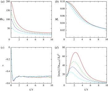
in figure 1. During an initial transition period (up to
 $2{-}3{\it\tau}$
), the energy is redistributed across scales by nonlinear energy transfer mechanisms, resulting in a state of turbulence. Since the initial conditions are not in acoustic equilibrium, pressure fluctuations develop from the initial field as the pressure becomes consistent with the velocity (Ristorcelli & Blaisdell Reference Ristorcelli and Blaisdell1997). The enstrophy increases as the fluctuations representing the different turbulent modes (acoustic, vorticity and entropy) reach this equilibrium state (Monin & Yaglom Reference Monin and Yaglom1975). The skewness of velocity derivatives, defined as
 $$\begin{eqnarray}S=\frac{\displaystyle \left\langle \frac{1}{3}\left(\frac{\partial u_{i}}{\partial x_{i}}\right)^{3}\right\rangle _{vol}}{\displaystyle \left\langle \frac{1}{3}\left(\frac{\partial u_{i}}{\partial x_{i}}\right)^{2}\right\rangle _{vol}^{1.5}},\end{eqnarray}$$
is a measure of the nonlinear equilibrium of turbulence; in our simulations, it ranges between
 $-$
0.6 and
 $-$
0.4 at
 $\mathit{Re}_{{\it\lambda},o}=60{-}200$
, in agreement with previously reported values for physically realistic turbulence (Sreenivasan & Antonia Reference Sreenivasan and Antonia1997). Since there is no external forcing providing energy to the turbulence, the total kinetic energy decays due to viscous diffusion, as exemplified by the decrease in turbulent Mach number. As is the case in many past numerical studies of this problem (Lee et al.
Reference Lee, Lele and Moin1991; Larsson & Lele Reference Larsson and Lele2009; Johnsen et al.
Reference Johnsen, Larsson, Bhagatwala, Cabot, Moin, Olson, Rawat, Shankar, Sjogreen, Yee, Zhong and Lele2010; Bhagatwala & Lele Reference Bhagatwala and Lele2011, Reference Bhagatwala and Lele2012), the Reynolds numbers do not remain over 100 for an extensive time in our simulations, such that the turbulence is not fully developed based on the definition of Dimotakis (Reference Dimotakis2000). In this sense, we do not expect our results to be Reynolds-number independent. Although shocklets may form at sufficiently high
 $M_{t}$
and thus require shock capturing, the present focus is on
 $M_{t}<0.4$
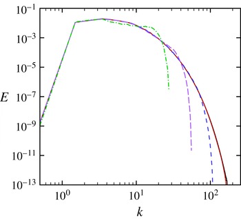
(Samtaney, Pullin & Kosovic Reference Samtaney, Pullin and Kosovic2001); for the present turbulent Mach numbers, central differences can be used in a stable fashion everywhere for all time. Turbulent kinetic energy spectra for
 $\mathit{Re}_{{\it\lambda},o}=100$
,
 $M_{t}=0.1$
and
 $t=4{\it\tau}$
are shown in figure 2 for different grid resolutions. These results confirm that the dynamics of all turbulent scales are accurately represented on a grid of
 $N^{3}=256^{3}$
, which is used for most of the present simulations.
Temporal evolution of
 $\mathit{Re}_{{\it\lambda}}$
(a),
 $M_{t}$
(b), skewness (c) and enstrophy (d) for single-fluid decaying isotropic turbulence at
 $\mathit{Re}_{{\it\lambda},o}=60$
(dot-dashed, cyan), 100 (long dashed, blue), 140 (short dashed, green) and 200 (solid, red).

Kinetic energy spectra for single-fluid decaying isotropic turbulence at
 $t=4{\it\tau}$
, with
 $\mathit{Re}_{{\it\lambda},o}=100$
,
 $M_{t}=0.1$
, and
 $N^{3}=32^{3}$
(dot-dashed, green),
 $64^{3}$
(long dashed, purple),
 $128^{3}$
(short dashed, blue),
 $256^{3}$
(dotted, red),
 $512^{3}$
(solid, black), where
 $N$
is the number of grid points per domain width. Note that the red and black curves lie on top of each other.

2.4. Initial set-up for the multifluid simulations
2.4.1. Domain and initial mass fraction field
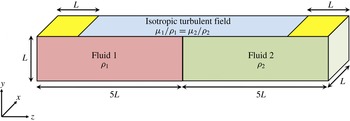
The computational domain consists of a rectangular parallelepiped of size
 $L\times L\times 10L$
, with
 $L=2{\rm\pi}$
and
 $N$
points per
 $L$
on a uniform Cartesian grid (figure 3). The velocity field described in § 2.3 is used to initialise the problem. Taking advantage of periodicity, 10 such isotropic boxes are juxtaposed in the
 $z$
direction to make up the full domain. Boundary conditions are periodic in the
 $x$
and
 $y$
directions, and non-reflecting with one-sided differences in the
 $z$
direction. Although the approach of Thompson (Reference Thompson1987) is followed for non-reflecting conditions, numerical errors may be generated as turbulence reaches the boundaries. To avoid such difficulties, an error function is used to damp the turbulent fluctuations near the boundaries. The length of the domain
 $(10L)$
in the
 $z$
direction is selected to ensure that boundaries have a negligible effect on the evolution of the mixing region near
 $z=0$
.
Schematic of the initial computational set-up (not to scale). Two fluids of different densities are initially separated by a diffuse unperturbed material interface in the presence of a random initial velocity field that evolves to turbulence. The turbulence is damped in the yellow region to avoid numerical errors at the non-reflecting boundaries.

To prevent generation of unphysical waves at the interface in the presence of finite physical mass diffusion, the following mean velocity is prescribed at the interface (Joseph Reference Joseph1990; Cook & Dimotakis Reference Cook and Dimotakis2001; Movahed Reference Movahed2014),
 $$\begin{eqnarray}u_{i}=-\frac{1}{\mathit{Re}\,\mathit{Sc}}\frac{1}{{\it\rho}}\frac{\partial {\it\rho}}{\partial x_{i}}.\end{eqnarray}$$
While the initial volume-averaged velocity is homogeneous and isotropic, inhomogeneity is introduced in the form of composition and density gradients in the
 $z$
direction. The initial mass fraction field is generated without any perturbations in the
 $x{-}y$
plane:
 $$\begin{eqnarray}Y_{1}(z)=\frac{1}{2}\left[1-\text{erf}\!\left(\frac{z-z_{0}}{H}\right)\right],\end{eqnarray}$$
where
 $z_{0}=0$
is the mid-plane location separating the two fluids corresponding to
 $Y_{1}=0.5$
. The value
 $H=8/128L$
corresponds to the steepest interface profile that central differences are capable of resolving in a satisfactory fashion on a
 $N=128$
points per
 $L$
grid, thus avoiding the use of shock capturing and minimising numerical dissipation that would otherwise overwhelm the small turbulent scales (Johnsen et al.
Reference Johnsen, Larsson, Bhagatwala, Cabot, Moin, Olson, Rawat, Shankar, Sjogreen, Yee, Zhong and Lele2010). Because of this, the mixing region has a finite initial size. For simplicity, we keep the ratio of the initial thickness of the mixing region to the initial Taylor microscale constant for all simulations. In the current set-up, pressure is uniform initially. To achieve an isothermal field and minimise compressibility effects, the properties of the heavy and light fluids are related as follows (Dimonte et al.
Reference Dimonte, Youngs, Dimits, Weber, Marinak, Wunsch, Garasi, Robinson, Andrews, Ramaprabhu, Calder, Fryxell, Biello, Dursi, MacNeice, Olson, Ricker, Rosner, Timmes, Tufo, Young and Zingale2004):
 $$\begin{eqnarray}\frac{R_{2}}{R_{1}}=\frac{M_{1}}{M_{2}}=\frac{{\it\rho}_{1}}{{\it\rho}_{2}},\quad p_{initial}=T_{initial}=2{\rm\pi}L({\it\rho}_{1}+{\it\rho}_{2}).\end{eqnarray}$$
In the mixing region, the initial density profile is obtained from the mass fraction field (Cook & Dimotakis Reference Cook and Dimotakis2001):
 $$\begin{eqnarray}\frac{1}{{\it\rho}}=\frac{Y_{1}}{{\it\rho}_{1}}+\frac{Y_{2}}{{\it\rho}_{2}}.\end{eqnarray}$$
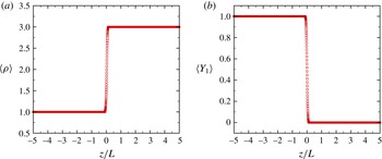
Figure 4 shows the initial mass fraction and density fields for
 ${\it\rho}_{2}/{\it\rho}_{1}=3$
.
Initial mass fraction (a) and density (b) fields for
 $N=256$
per
 $L$
and
 ${\it\rho}_{2}/{\it\rho}_{1}=3$
.

2.4.2. Matched dissipation rate and key dimensionless parameters
The important parameters in the heavy and light fluids are related as follows:
 $$\begin{eqnarray}\frac{\mathit{Re}_{{\it\lambda}2}}{\mathit{Re}_{{\it\lambda}1}}=\frac{{\it\rho}_{2}{\it\mu}_{1}}{{\it\rho}_{1}{\it\mu}_{2}},\quad M_{t2}=M_{t1}\sqrt{\frac{{\it\rho}_{2}}{{\it\rho}_{1}}},\end{eqnarray}$$
with
 $M_{t1}=0.1$
. Due to the non-dimensionalisation, the turbulent Mach number is slightly different in each fluid, but since dilatational dissipation is negligible this discrepancy is not expected to affect the dynamics. Simulations are performed at a Prandtl number of 0.7 and Schmidt number 1.0.
The fluids have different densities and dynamic viscosities such that the kinematic viscosities are the same in both fluids, i.e.
 ${\it\mu}_{1}/{\it\rho}_{1}={\it\mu}_{2}/{\it\rho}_{2}$
. Since the velocity is initialised with the same random field in each fluid, the initial Taylor-scale Reynolds numbers are the same in both fluids. Furthermore, we expect the integral quantities representative of the turbulence dynamics, e.g. dissipation rate, enstrophy and turbulent kinetic energy per unit mass, and relevant length scales (Taylor and Kolmogorov microscales) to evolve in the same fashion in each fluid, except perhaps in the mixing region (Samtaney et al.
Reference Samtaney, Pullin and Kosovic2001; Movahed & Johnsen Reference Movahed and Johnsen2013b
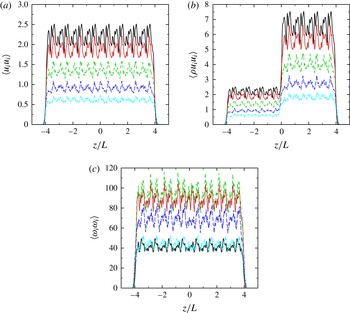
). Therefore, the initial conditions exhibit anisotropy solely in the composition and density gradients. Figure 5 confirms that the kinetic energy per unit mass
 $\langle u_{i}u_{i}\rangle$
and enstrophy remain nearly uniform in the entire domain apart from slight changes in the mixing region for a density ratio of 3:1. Since it is not possible to simultaneously match the kinetic energy per unit mass and the kinetic energy per unit volume
 $\langle {\it\rho}u_{i}u_{i}\rangle$
when considering fluids of different densities, we choose to match the kinetic energy per unit mass in this study. The rationale behind this strategy is that conventional turbulence scalings are based on kinetic energy per unit mass and kinematic viscosity, such that density and dynamic viscosity do not appear. Thus, by matching the initial kinematics (kinetic energy per unit mass) and the corresponding dissipation (kinematic viscosity) in the two fluids, the turbulence decays at the same rate in the two fluids, even though there is an initial gradient in the kinetic energy (per unit volume). The present problem set-up to investigate the role of density gradient alone is justified by the nearly homogeneous kinetic energy per unit mass and enstrophy in figure 5, even across the mixing region. The density difference across the interface manifests itself as a gradient in the turbulent kinetic energy per unit volume across the mixing region, as shown in figure 5. This gradient in the mass-averaged kinetic energy across the mixing region decreases as turbulence decays.
Spatial distribution of the kinetic energy per unit mass and per unit volume and enstrophy in the
 $x{-}y$
plane during the first four eddy turnover times for
 $\mathit{Re}_{{\it\lambda},o}=100$
,
 ${\it\rho}_{2}/{\it\rho}_{1}=3$
, and
 $t/{\it\tau}=0$
(solid, black), 1 (dotted, red), 2 (short dashed, green), 3 (long dashed, blue) and 4 (dot-dashed, cyan).

To show that the turbulence dynamics are similar at different densities, we conduct two simulations of single-fluid decaying isotropic turbulence, one with an initial uniform density of one and another with an initial uniform density of three. The respective viscosities are chosen such that
 $\mathit{Re}_{{\it\lambda},o}=100$
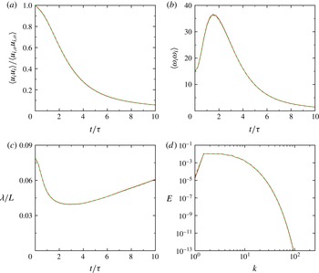
in both simulations. These two simulations correspond to freely decaying turbulence in the multifluid set-up with a density ratio of three away from the interface in the light and heavy fluids. Figure 6 shows the temporal evolution of volume-averaged kinetic energy per unit mass, enstrophy, Taylor microscale, and velocity spectra at
 $t/{\it\tau}=10$
. These results confirm that by matching the kinematic viscosity the turbulence, created by the initial field behaves in the same fashion in a light and in a heavy fluid. The slight difference between the two results is due to the different initial turbulent Mach numbers (2.20).
Temporal evolution of normalised kinetic energy per unit mass, enstrophy and Taylor microscale, and kinetic energy spectra at
 $t/{\it\tau}=10$
for
 $\mathit{Re}_{{\it\lambda},o}=100$
, and initial densities of 1 (solid, red) and 3 (dashed, green) with the same kinematic viscosity.

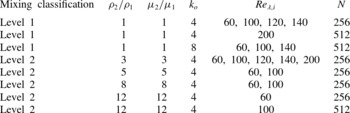
In our simulations, the quantities that we vary are the density ratio,
 ${\it\rho}_{2}/{\it\rho}_{1}=1$
, 3, 5, 8 and 12, and the initial Reynolds numbers,
 $\mathit{Re}_{{\it\lambda},o}=60$
, 100, 120, 140 and 200. A density ratio of
 ${\it\rho}_{2}/{\it\rho}_{1}=1$
corresponds to passive scalar mixing, since the other relevant fluid properties are identical. Table 1 summarises the simulations runs, along with the relevant flow parameters.
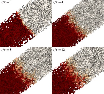
Snapshots of turbulent eddies extracted by the normalised
 $Q$
-criterion coloured by mass fraction for
 $\mathit{Re}_{{\it\lambda},o}=100$
and
 ${\it\rho}_{2}/{\it\rho}_{1}=3$
. Dark red, light fluid (bottom left); white, heavy fluid (top right).

Summary of the DNS runs with the relevant flow parameters.

3. Results: dynamics of the large scales in the mixing region
The focus of this section lies in the large-scale dynamics of the mixing region. First, the qualitative behaviour is presented (§ 3.1). For different density ratios, we consider the evolution of the mixing region width in § 3.2, followed by analysis based on the observation that the growth is self-similar (§ 3.3). We finally assess how well mixed the fluids are in § 3.4.
3.1. Qualitative behaviour of the large scales
We begin by considering the qualitative behaviour of the velocity and mass fraction fields. Figure 7 shows instantaneous three-dimensional visualisations of the evolution of the turbulent field and mixing region for
 ${\it\rho}_{2}/{\it\rho}_{1}=3$
and
 $\mathit{Re}_{{\it\lambda},o}=100$
, where
 $\mathit{Re}_{{\it\lambda}}$
is the initial Taylor-scale Reynolds number. The normalised
 $Q$
-criterion is defined as
 $$\begin{eqnarray}{\it\Lambda}=\frac{\unicode[STIX]{x1D61A}_{ij}^{\ast }\unicode[STIX]{x1D61A}_{ij}^{\ast }-{\textstyle \frac{1}{2}}{\it\omega}_{k}{\it\omega}_{k}}{\unicode[STIX]{x1D61A}_{ij}^{\ast }\unicode[STIX]{x1D61A}_{ij}^{\ast }+{\textstyle \frac{1}{2}}{\it\omega}_{k}{\it\omega}_{k}},\end{eqnarray}$$
where
 ${\bf\omega}=\boldsymbol{{\rm\nabla}}\times \boldsymbol{u}$
is the vorticity and
 $$\begin{eqnarray}\unicode[STIX]{x1D61A}_{ij}^{\ast }=\unicode[STIX]{x1D61A}_{ij}-\frac{{\it\delta}_{ij}}{3}\unicode[STIX]{x1D61A}_{kk},\quad \unicode[STIX]{x1D61A}_{ij}=\frac{1}{2}\left(\frac{\partial u_{i}}{\partial x_{j}}+\frac{\partial u_{j}}{\partial x_{i}}\right),\end{eqnarray}$$
where
 $\unicode[STIX]{x1D61A}_{ij}$
is the strain-rate tensor. The
 $Q$
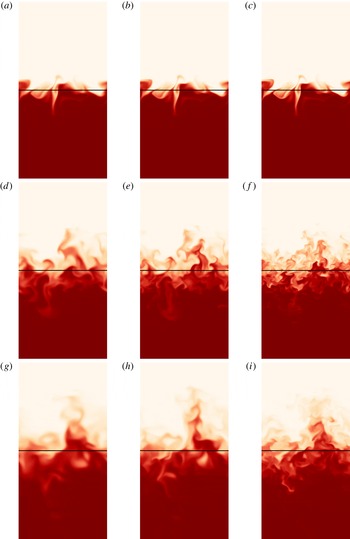
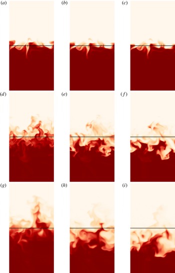
-criterion is used to extract approximate outlines of the turbulent eddies and visualise changes in their morphology. In addition, the eddies are coloured by mass fraction to highlight the dynamics and growth of the mixing region. Over the first few eddy turnover times, ever smaller scales are produced as the energy is redistributed across wavenumbers and the initial random field evolves to turbulence. At late times, the smaller eddies have dissipated, leaving the largest ones behind (Pope Reference Pope2000). The mixing region grows with time through a turbulent diffusion process, in which heavy eddies near the interface are entrained and dispersed into the light fluid, and vice versa. There is no clear qualitative difference between the size and dynamics of eddies at any fixed time in the flow. Similar observations can be made by considering instantaneous two-dimensional slices of mass fraction in figures 8 and 9. As the Reynolds number is increased, smaller-scale features are discernible at a given time; however, it is not immediately clear how the Reynolds number affects the mixing region growth rate. A larger density ratio does not appear to significantly affect the size distribution of the turbulent length scales qualitatively. However, the mean location of the mixing region changes in the plots for different density ratios; the heavier fluid displaces the lighter. In addition, this process appears to produce a wider mixing region. Although such qualitative results provide useful information, more quantitative measures are necessary, which are investigated in greater detail in the following sections.
Two-dimensional contours of mass fraction in the
 $x{-}z$
plane at
 $t=1{\it\tau}$
(a,b,c),
 $t=5{\it\tau}$
(d,e,f) and
 $t=10{\it\tau}$
(g,h,i) for
 ${\it\rho}_{2}/{\it\rho}_{1}=1$
and
 $\mathit{Re}_{{\it\lambda},o}=60$
(a,d,g), 100 (b,e,h) and 200 (c,f,i). The vertical direction corresponds to the direction of anisotropy in the composition (
 $z$
direction). Each plot covers an area of
 $L\times 2L$
and the initial mid-plane (
 $z=0$
) is located in the middle of the vertical direction. Dark red, light fluid (bottom); white, heavy fluid (top); black line, initial
 $z=0$
plane.

Two-dimensional contours of mass fraction in the
 $x{-}z$
plane at
 $t=1{\it\tau}$
(a–c),
 $t=5{\it\tau}$
(d–f) and
 $t=10{\it\tau}$
(g-i) for
 $\mathit{Re}_{{\it\lambda},o}=100$
and
 ${\it\rho}_{2}/{\it\rho}_{1}=1$
(a,d,g), 5 (b,e,h) and 12 (c,f,i). The vertical direction corresponds to the direction of anisotropy in the composition (
 $z$
direction). Each plot covers an area of
 $L\times 2L$
and the initial mid-plane (
 $z=0$
) is located in the middle of the vertical direction. Dark red, light fluid (bottom); white, heavy fluid (top); black line, initial
 $z=0$
plane.

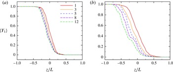
Mass fraction profiles at
 $t=3{\it\tau}$
(a) and
 $t=10{\it\tau}$
(b) for
 $\mathit{Re}_{{\it\lambda},o}=100$
, and
 ${\it\rho}_{2}/{\it\rho}_{1}=1$
(solid, red), 3 (dotted, orange), 5 (short dashed, blue), 8 (long dashed, purple) and 12 (dot-dashed, green).

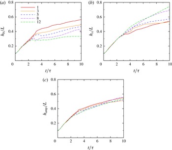
Temporal evolution of (a)
 $h_{b}$
, (b)
 $h_{s}$
and (c)
 $h_{amp}$
for
 $\mathit{Re}_{{\it\lambda},o}=100$
, and
 ${\it\rho}_{2}/{\it\rho}_{1}=1$
(solid, red), 3 (dotted, orange), 5 (short dashed, blue), 8 (long dashed, purple) and 12 (dot-dashed, green).

3.2. Evolution of the mixing region width
The dynamics in the mixing region are of particular interest, so instantaneous mean profiles of mass fraction are first examined. As the fluids mix, the width of the mixing region grows with time. The temporal evolution of the mass fraction varies with density ratio, as shown in figure 10. More importantly, the mid-plane corresponding to
 $\langle Y\rangle =0.5$
, where
 $\langle \cdot \rangle$
denotes spatial averages in
 $x{-}y$
, shifts toward the lighter fluid as the density ratio is increased; we discuss this phenomenon in more detail at the end of this section. This result is important in the context of the Rayleigh–Taylor instability, as the temporal evolution of turbulence statistics is often reported at a fixed location relative to the grid, namely the
 $z=0$
plane (Cook & Dimotakis Reference Cook and Dimotakis2001). The mass fraction is essentially antisymmetric about
 $\langle Y\rangle =0.5$
at low-density ratios, but loses this property as the density ratio increases.
Temporal evolution of spike amplitude for
 $\mathit{Re}_{{\it\lambda},o}=100$
,
 ${\it\rho}_{2}/{\it\rho}_{1}=3$
(solid, orange) and 8 (dashed curve, purple) for different initial thicknesses
 $H$
as defined in (2.17): (a)
 $H=8/128L$
, used in the rest of the article; (b)
 $H=1/128L$
.

Temporal evolution of the
 $\langle Y\rangle =0.5$
plane in
 $z$
for
 $\mathit{Re}_{{\it\lambda},o}=100$
, and
 ${\it\rho}_{2}/{\it\rho}_{1}=1$
(solid, red), 3 (dotted, orange), 5 (short dashed, blue), 8 (long dashed, purple) and 12 (dot-dashed, green).

We measure the mixing region growth using two approaches. The first, borrowed from Rayleigh–Taylor instability analysis, is based on the notion of spikes/bubbles (masses of heavy/light fluids penetrating the light/heavy fluids). The spike (bubble) amplitude
 $h_{s}$
(
 $h_{b}$
) is defined as the distance between
 $\langle Y_{1}\rangle \leqslant 0.99$
(
 $\langle Y_{1}\rangle \geqslant 0.01$
) and the initial mid-plane (
 $z=0$
). The spikes (bubbles) amplitude growth is due to the penetration of the heavy (light) fluid into the light (heavy) fluid. The amplitude of the mixing region,
 $h_{amp}$
is defined as the average of
 $h_{b}$
and
 $h_{s}$
:
 $$\begin{eqnarray}h_{amp}=\frac{h_{s}+h_{b}}{2}.\end{eqnarray}$$
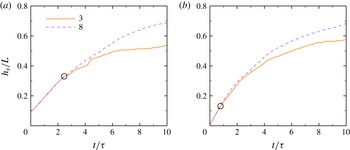
Figure 11 shows that over the first two to three eddy turnover times different density ratios do not produce very different
 $h_{s}$
or
 $h_{b}$
; this observation can be related to the initial thickness of the unperturbed interface at
 $t=0$
. Since the initial Taylor microscale is on the order of the initial interface thickness, it takes finite time for the eddies in the pure heavy fluid to penetrate the pure light fluid and contribute to spike growth. This behaviour occurs sooner for simulations with an initially thinner interface (figure 12), in which case the role of the density gradient on the bubble and spike growth becomes evident from earlier times. After the first two to three eddy turnover times, the growth of the bubbles and spikes strongly depend on the density ratio (figure 11). The increase in spike amplitude can be explained via momentum considerations. In the absence of gravity and with increasing
 ${\it\rho}_{2}/{\it\rho}_{1}$
, an eddy in the heavy fluid has higher momentum than the corresponding volume of light fluid, such that it is easier for the heavy fluid to displace the light fluid and penetrate it. The same dependence on the density ratio (through the Atwood number) has been observed in Rayleigh–Taylor instability (Cook & Dimotakis Reference Cook and Dimotakis2001). The asymmetry in bubble/spike growth in the absence of gravity suggests that such momentum considerations are important factors in the asymmetric growth observed in Rayleigh–Taylor instability as
 ${\it\rho}_{2}/{\it\rho}_{1}$
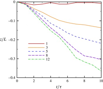
is increased, rather than gravity effects alone. As a result, the mean position of the interface moves toward the light fluid. This motion is greater for higher density ratio, an observation confirmed by monitoring the location in
 $z$
of the
 $\langle Y\rangle =0.5$
plane (figure 13). To illustrate this point, we extend the analysis of Tordella, Iovieno & Bailey (Reference Tordella, Iovieno and Bailey2008) to variable-density flows. Assuming that the dilatation is small in our problem, the averaged momentum equations can be written
 $$\begin{eqnarray}\frac{\partial \overline{{\it\rho}u_{i}}}{\partial t}+\frac{\partial }{\partial x_{j}}\overline{{\it\rho}u_{i}u_{j}}=-\frac{\partial \bar{p}}{\partial x_{j}}+\frac{\partial }{\partial x_{j}}\overline{\left({\it\mu}\frac{\partial u_{i}}{\partial x_{j}}\right)},\end{eqnarray}$$
where the bars denote the mean. Since there is no mean pressure gradient, the
 $z$
-momentum equation for the mean reduces to
 $$\begin{eqnarray}\frac{\partial }{\partial t}\overline{{\it\rho}w}=-\frac{\partial }{\partial z}\overline{{\it\rho}w^{2}}+\frac{\partial }{\partial z}\overline{{\it\mu}\frac{\partial w}{\partial z}}.\end{eqnarray}$$
Initially, the mean momentum is zero. Since the last term is diffusive, the mean momentum in the
 $z$
direction becomes negative for a positive density gradient, such that the mean interface location moves in the negative
 $z$
direction, thus confirming the simulations results. Over the range
 $1\lesssim t/{\it\tau}\lesssim 4$
, the mean interface location appears to move at an approximately constant velocity proportional to the Atwood number, although the explicit dependence is not straightforward. While this motion results in a greater asymmetry in bubble and spike as the density ratio increases, it does not have a clear effect on the total mixing width (
 $2h_{amp}$
) as the asymmetry is de-emphasised when averaging the bubble and spike growth in (3.3). For
 $4\lesssim t/{\it\tau}\lesssim 6$
, the higher density ratios lead to a smaller
 $h_{amp}$
; no clear pattern emerges thereafter.
The second measure of mixing region width is defined as
 $$\begin{eqnarray}h=2\int _{-\infty }^{\infty }\min (\langle Y_{1}\rangle ,\langle Y_{2}\rangle )\,\text{d}z,\end{eqnarray}$$
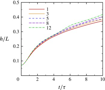
and is preferred for analysing the growth rate compared with (3.3) since it has the advantage of avoiding dependence on statistical fluctuations (Cook & Dimotakis Reference Cook and Dimotakis2001; Cabot & Cook Reference Cabot and Cook2006; Cabot & Zhou Reference Cabot and Zhou2013). Figure 14 shows
 $h$
for different
 ${\it\rho}_{2}/{\it\rho}_{1}$
. In this case, a larger density ratio contributes to a larger mixing region width, consistent with the contour plots in § 3.1. The behaviour of
 $h$
defined in (3.6) is analysed in the next section.
Temporal evolution of the mixing region width
 $h$
based on (3.6) for
 $\mathit{Re}_{{\it\lambda},o}=100$
, and different
 ${\it\rho}_{2}/{\it\rho}_{1}$
.

3.3. Self-similarity and scaling of the mixing region width
The scaling of the mixing region width
 $h$
with time is a quantity of practical engineering importance. With the present problem set-up, turbulent diffusion of a passive scalar, i.e.
 ${\it\rho}_{2}={\it\rho}_{1}$
, is expected to be a self-similar process with the same growth rate in each
 $z$
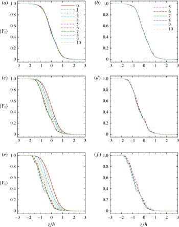
direction since the dissipation rate, and thus the turbulence, are identical in each fluid. This behaviour is confirmed for all density ratios by plotting the average mass fraction field as a function of the similarity variable
 ${\it\xi}=z/h$
in figure 15. As the density ratio is increased, self-similarity is still observed, though it takes longer to develop and in the most mixed regions (
 $0.4\lesssim \langle Y\rangle \lesssim 0.6$
) the profiles do not perfectly collapse at the higher density ratios.
Average mass fraction field in the
 $x{-}y$
plane at different times for
 $\mathit{Re}_{{\it\lambda},o}=100$
and
 ${\it\rho}_{2}/{\it\rho}_{1}=1$
(a,b), 5 (c,d) and 12 (e,f): (a,c,e)
 $0{-}10{\it\tau}$
; (b,d,f):
 $5{-}10{\it\tau}$
.

We seek to determine the scaling of
 $h$
with time. This mixing process can be described by one-dimensional (turbulent) diffusion of one fluid into the other:
 $$\begin{eqnarray}\frac{\partial Y}{\partial t}=\frac{\partial }{\partial z}\left({\it\kappa}\frac{\partial Y}{\partial z}\right),\end{eqnarray}$$
where
 $Y$
is the mass fraction and
 ${\it\kappa}$
is an effective diffusion coefficient that varies with time and may be Reynolds-number dependent. After integrating (3.7) for
 $z<0$
, and rearranging following Lawrie & Dalziel (Reference Lawrie and Dalziel2011), we obtain
 $$\begin{eqnarray}h{\dot{h}}={\it\kappa}\left(\frac{\displaystyle \left.\frac{\partial Y}{\partial {\it\xi}}\right|_{{\it\xi}=0}}{\displaystyle -\!\int _{-\infty }^{0}Y({\it\xi})\,\text{d}{\it\xi}}\right).\end{eqnarray}$$
Since the expression in parentheses is a constant,
 $h{\dot{h}}\sim {\it\kappa}$
. To determine
 ${\it\kappa}$
, Prandtl’s mixing length theory,
 ${\it\kappa}\sim u_{turb}l_{turb}$
, is invoked, where
 $u_{turb}=u_{rms}$
,
 $l_{turb}={\it\lambda}$
, where
 ${\it\lambda}$
is the Taylor microscale. Since
 ${\it\mu}/{\it\rho}$
is the same for both fluids,
 ${\it\kappa}\sim \mathit{Re}_{{\it\lambda}}$
. Theoretical self-preserving analysis as well as grid turbulence experiments for a decaying isotropic field (George Reference George1992) support the following scalings:
 $$\begin{eqnarray}{\it\lambda}\sim t^{1/2},\quad u_{rms}^{2}\sim t^{-n}.\end{eqnarray}$$
Thus,
 $\mathit{Re}_{{\it\lambda}}\sim t^{(1-n)/2}$
. Defining
 ${\it\alpha}=(1-n)/2$
, the power-law behaviour of
 $\mathit{Re}_{{\it\lambda}}\sim t^{{\it\alpha}}$
yields the following scaling for the mixing region width:
 $$\begin{eqnarray}h\sim t^{({\it\alpha}+1)/2}\sim t^{1-n/2}.\end{eqnarray}$$
The same scaling of the mixing region with time can be obtained by other approaches (e.g. that of Layzer (Reference Layzer1955) or simple control volume analysis), with the key assumption being that the kinetic energy decays as a power law with respect to time. We note that according to Dimotakis (Reference Dimotakis2000) the turbulence is not fully developed in the self-similar regime (recall figure 1) since
 $\mathit{Re}_{{\it\lambda}}$
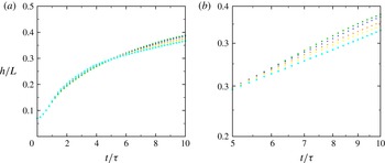
falls below 100 for the major part of our simulations, such that Reynolds-number dependence is expected in this scaling. These observations are confirmed in figure 16, although the sensitivity to the Reynolds number is relatively weak. This can be explained by noticing that the difference in
 $\mathit{Re}_{{\it\lambda}}$
is less than 25 at any time during the self-similar regime for the present initial Taylor-scale Reynolds numbers (
 $60\leqslant \mathit{Re}_{{\it\lambda},o}\leqslant 200$
). This small change in
 ${\it\alpha}$
does not significantly affect
 $h$
.
Time evolution of the mixing region width (with
 ${\it\rho}_{2}/{\it\rho}_{1}=3$
) for
 $\mathit{Re}_{{\it\lambda},o}=60$
(squares, green), 100 (upward-pointing triangles, blue), 120 (downward-pointing triangles, orange), 140 (diamonds, yellow) and 200 (circles, cyan): (a) linear–linear; (b) log–log.

3.3.1. High-Reynolds-number limit
This analysis can be taken one step further by assuming fully developed turbulence, in which case we can compute the actual exponent based on energy considerations previously used for Rayleigh–Taylor turbulence near bubbles and spikes (Abarzhi, Gorobets & Sreenivasan Reference Abarzhi, Gorobets and Sreenivasan2005). Grid turbulence experiments of decaying homogeneous isotropic turbulence support the following empirical law (Comte-Bellot & Corrsin Reference Comte-Bellot and Corrsin1966) for the velocity fluctuations:
 $$\begin{eqnarray}\frac{\text{d}u^{2}}{\text{d}t}\sim -\frac{u^{3}}{l},\end{eqnarray}$$
where
 $l$
is the integral scale. A fluid parcel initially at the interface is transported by eddies of different sizes in the fluctuating velocity field
 $u$
. The largest eddies of size
 $l$
contribute the most to the growth of the mixing region, thus suggesting a scaling
 $h\sim l$
. This scaling is in agreement with the water tunnel grid-generated turbulence experiments of Huq & Britter (Reference Huq and Britter1995a
). The dynamics of the mixing region can also be related to the fluctuating field as
 ${\dot{h}}\sim u$
. For the Batchelor spectrum considered here,
 $u^{2}l^{5}$
is an invariant, which corresponds to conservation of angular momentum (Batchelor & Proudman Reference Batchelor and Proudman1956). Substituting into (3.11) yields
 $$\begin{eqnarray}u^{2}\sim t^{-10/7},\quad h\sim l\sim t^{2/7}.\end{eqnarray}$$
This result provides an asymptotic limit for the exponent in fully developed (Reynolds-number-independent) turbulence starting from a Batchelor spectrum.
3.3.2. Comparison between theory and simulations
The above arguments can be verified by comparing
 $h(t)$
computed directly from the DNS with that obtained by measuring
 ${\it\alpha}$
from
 $\mathit{Re}_{{\it\lambda}}(t)$
and substituting into (3.10). A power-law least-squares fit to
 $\mathit{Re}_{{\it\lambda}}$
in the mixing region is performed to find
 ${\it\alpha}$
at different
 $\mathit{Re}_{{\it\lambda},o}$
. To compute
 $h$
, we use the regression method of Krogstad & Davidson (Reference Krogstad and Davidson2010). The process relies on a linear best fit for
 $$\begin{eqnarray}\ln h=\ln (a)+n\ln (t-t_{0}),\end{eqnarray}$$
where
 $t_{0}$
is the virtual point of origin. Assuming that
 $d_{i}$
is the fitted function, for each
 $t_{0}$
the variance can be defined as
 $$\begin{eqnarray}{\it\sigma}^{2}=\frac{1}{N-1}\mathop{\sum }_{i=1}^{N}[d_{i}(x_{i})-h(x_{i})]^{2}.\end{eqnarray}$$
We consider
 $t_{0}/{\it\tau}=0.0$
, 0.5, 1.0, 1.5 and 2.0. Since
 $t_{0}/{\it\tau}=0.0$
and 0.5 yield the smallest
 ${\it\sigma}^{2}$
, we report data corresponding to these two values. As described in § 2.3, it takes approximately
 $2{\it\tau}$
for the initial field to evolve to turbulence; additional time is expected to be required for the mass fraction field to become correlated with the velocity field and result in self-similar growth, as supported by figure 15 in which the data collapses well between 5 and
 $10{\it\tau}$
. Thus, we pick
 $t=5{\it\tau}$
as a safe choice for the beginning of the self-similar regime in our analysis and take
 $t=10{\it\tau}$
as the final time to prevent box-size effects. The growth obtained using the two different approaches (directly from the DNS versus computing
 ${\it\alpha}$
from
 $\mathit{Re}_{{\it\lambda}}$
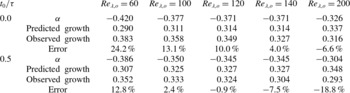
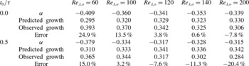
) is compared in table 2 for
 ${\it\rho}_{1}/{\it\rho}_{2}=1$
and table 3 for
 ${\it\rho}_{1}/{\it\rho}_{2}=3$
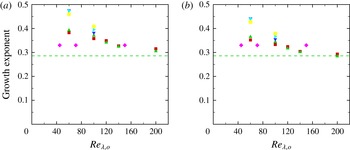
, and figure 17 shows the exponent of time for different
 $\mathit{Re}_{{\it\lambda},o}$
and density ratios. The exponents lie in the range 0.29–0.38 for a density ratio of 1 and 0.28–0.39 for a density ratio of 3; overall, the agreement between the two different approaches for measuring the time exponent is good. The general trend shows that the growth exponent decreases as
 $\mathit{Re}_{{\it\lambda},o}$
increases, and in fact tends to the asymptotic limit of fully developed turbulence (3.12). The discrepancy in the growth exponent decreases as
 $\mathit{Re}_{{\it\lambda},o}$
increases up to 140. The decrease in the growth of the mixing region likely is related to the higher enstrophy (i.e. dissipation) at higher
 $\mathit{Re}_{{\it\lambda},o}$
during the self-similar regime. Figure 17 suggests that the growth exponent, and thus mixing region width, increases with the density ratio for a given
 $\mathit{Re}_{{\it\lambda},o}$
, but this dependence is not completely monotonic. As discussed in § 3.2, for a density ratio of one, the mixing region grows symmetrically in both fluids. At higher density ratios, the mixing region grows asymmetrically as an eddy in the heavy fluid has higher momentum than the corresponding volume of light fluid, such that it is easier for the heavy fluid to displace the light fluid and penetrate it. By the same argument, it is more difficult for the light fluid to penetrate the heavy fluid.
Scaling of
 $h$
with time for
 ${\it\rho}_{2}/{\it\rho}_{1}=1$
, and virtual origins
 $t_{0}/{\it\tau}=0.0$
and 0.5. The predicted growth
 $({\it\alpha}+1)/2$
is obtained using (3.10) by fitting
 $\mathit{Re}_{{\it\lambda}}\sim t^{{\it\alpha}}$
. The observed growth is calculated by performing a direct data fit to
 $h$
. The same interval
 $(5{-}10{\it\tau})$
is used in each case to obtain
 ${\it\alpha}$
and the observed growth. The error is defined as (observed growth – predicted growth)/observed growth.

Time exponent of the mixing region width computed directly from the DNS:
 ${\it\rho}_{2}/{\it\rho}_{1}=1$
(squares, red), 3 (upward-pointing triangles, green), 5 (downward-pointing triangles, blue), 8 (rightward-pointing triangles, cyan) and 12 (circles, yellow): (a)
 $t_{0}/{\it\tau}=0.0$
; (b)
 $t_{0}/{\it\tau}=0.5$
. Purple diamonds: DNS of Tordella & Iovieno (Reference Tordella and Iovieno2011). Green dashed line: theoretical growth exponent of
 $2/7$
(3.12).

Scaling of
 $h$
with time for
 ${\it\rho}_{2}/{\it\rho}_{1}=3$
, and virtual origins
 $t_{0}/{\it\tau}=0.0$
and 0.5. The predicted growth
 $({\it\alpha}+1)/2$
is obtained using (3.10) by fitting
 $\mathit{Re}_{{\it\lambda}}\sim t^{{\it\alpha}}$
. The observed growth is calculated by performing a direct data fit to
 $h$
. The same interval
 $(5{-}10{\it\tau})$
is used in each case to obtain
 ${\it\alpha}$
and the observed growth. The error is defined as (observed growth – predicted growth)/observed growth.

The Batchelor spectrum is commonly used to initialise this problem in numerical simulations and is thus the focus of the present work. Nevertheless, the analysis for fully developed turbulence holds for other spectra, e.g. Saffman’s,
 $E(k)\sim k^{2}$
, in which case
 $u^{2}l^{3}$
is the relevant flow invariant (Saffman Reference Saffman1967). Starting from (3.11), a Saffman spectrum yields
 $h\sim l\sim t^{2/5}$
. For
 $\mathit{Re}_{{\it\lambda},o}=60,100,140$
and 200 and a virtual origin of
 $t_{0}=0$
, passive scalar simulations (
 ${\it\rho}_{2}/{\it\rho}_{1}=1$
) produce time exponents 0.44, 0.43, 0.39 and 0.37, respectively. Again, similar trends are observed, though the asymptotic limit slightly undershoots the prediction. We note that box-size effects become important earlier due to a more rapid growth with a Saffman spectrum and may thus reduce the computed exponent.
Our predicted values are consistent with past results, both experimental and computational. DNS of passive scalar mixing (Tordella & Iovieno Reference Tordella and Iovieno2011), in which isotropic turbulent fields with the same Taylor scale but different kinetic energy are juxtaposed, obtained a scaling
 $h\sim t^{0.33}$
based on multiple simulations with
 $\mathit{Re}_{{\it\lambda}}=45{-}150$
after the initial transient (Tordella & Iovieno Reference Tordella and Iovieno2011, figure 1). Our set-up is different, since the turbulent fields used here have the same volume-averaged kinetic energy per unit mass
 $u_{rms}^{2}/2$
but different kinetic energy per unit volume
 ${\it\rho}u_{rms}^{2}/2$
, which enables us to isolate the effect of the density gradient and investigate level 2 mixing. A
 $k$
–
 ${\it\epsilon}$
turbulent diffusion model (Anand & Pope Reference Anand and Pope1983) was used to predict a
 $t^{0.34}$
growth for experimental wind tunnels studies of the development of a thermal wake in an isotropic grid-generated turbulence behind a heated wire (Warhaft Reference Warhaft1984; Stapountzis et al.
Reference Stapountzis, Sawford, Hunt and Britter1986) at the last stage of the development of the thermal wake (turbulent diffusive stage). While the model of Anand & Pope (Reference Anand and Pope1983) fits the experimental data well, the slope of a power-law fit to the mixing region width does not reach the predicted growth. The observed time exponent for the growth of the mixing region in this study is close to those reported in studies of turbulent mixing following the Richtmyer–Meshkov instability after reshock (Tritschler et al.
Reference Tritschler, Olson, Lele, Hickel, Hu and Adams2014). This observation is expected, since the turbulence produced by such flows is very similar to that in the present study.
3.3.3. Effect of
 $k_{o}$

The ratio of the initial Taylor microscale
 $({\it\lambda}_{o}=2/k_{o})$
to the domain size
 $L$
is yet another parameter that enters the problem. In practice,
 $k_{o}=4$
is commonly used in studies of isotropic turbulence (Lee et al.
Reference Lee, Lele and Moin1991; Larsson & Lele Reference Larsson and Lele2009; Johnsen et al.
Reference Johnsen, Larsson, Bhagatwala, Cabot, Moin, Olson, Rawat, Shankar, Sjogreen, Yee, Zhong and Lele2010; Bhagatwala & Lele Reference Bhagatwala and Lele2011, Reference Bhagatwala and Lele2012). A higher
 $k_{o}$
is desirable to reduce box-size effects, as is sometimes done in Rayleigh–Taylor turbulence (Cabot & Cook Reference Cabot and Cook2006). In addition, putting the initial energy at higher modes allows for a more natural transition to a fully developed state from the initial artificial spectrum, specifically with regard to achieving a spectrum
 $E(k)\sim k^{4}$
at low wavenumbers. On the other hand, increasing
 $k_{o}$
significantly increases the required grid resolution. We performed most of our simulations with
 $k_{0}=4$
to resolve all scales on a grid of
 $N=256$
per
 $L$
. Here, we discuss the sensitivity of the results on
 $k_{o}$
by considering the passive scalar case (
 ${\it\rho}_{2}={\it\rho}_{1}$
) with
 $k_{0}=8$
and
 $\mathit{Re}_{{\it\lambda},o}=60{-}140$
on a grid of
 $N=512$
per
 $L$
. We set the initial thickness of the diffuse interface to be half that used for
 $k_{o}$
by doubling
 $H$
in (2.17), such that the ratio of
 ${\it\lambda}_{o}$
to the initial mixing thickness is the same as for
 $k_{o}=4$
. A corresponding self-similar behaviour is also observed for
 $k_{o}=8$
, with time exponents 0.335, 0.328 and 0.323 corresponding to
 $\mathit{Re}_{{\it\lambda},o}=60$
, 100 and 140, respectively. As for
 $k_{o}=4$
, the exponents decrease with increasing
 $\mathit{Re}_{{\it\lambda},o}$
, although at a reduced rate. Compared with the
 $k_{o}=4$
results, the mixing region width at
 $10{\it\tau}$
is half. Furthermore, the self-similar behaviour is observed up to
 $20{\it\tau}$
for
 $k_{o}=8$
, after which point box-size effects become evident. Thus, if one is interested in studying the problem until times later than
 $10{\it\tau}$
, higher values of
 $k_{o}$
should be considered to prevent box-size effects, although the computational cost is higher. The current data fit for
 $k_{0}=4$
is performed on the interval
 $5{\it\tau}<t<10{\it\tau}$
to avoid box-size effects and to remain in the self-similar regime. A longer period of self-similar behaviour in time compared with the current work would be desirable for a power-law fit.
3.4. Mixedness
Mixing can be quantified by considering a hypothetical reaction between two pure fluids where the fully mixed fluid is the product corresponding to a stoichiometric mixture of the two fluids (Cook & Dimotakis Reference Cook and Dimotakis2001). We use mass fraction for convenience instead of volume fraction typically used in the incompressible case. The mass fraction of the mixed fluid is
 $$\begin{eqnarray}Y_{m}(Y)=\left\{\begin{array}{@{}ll@{}}2Y\quad & \text{if }Y\leqslant 0.5,\\ 2(1-Y)\quad & \text{if }Y>0.5,\end{array}\right.\end{eqnarray}$$
where the stoichiometric coefficient is taken to be 0.5. The mixing region width (entrainment length) is defined as
 $$\begin{eqnarray}h_{m}=\int _{-\infty }^{\infty }Y_{m}(\langle Y\rangle )\,\text{d}z,\end{eqnarray}$$
where
 $h_{m}$
represents the maximum thickness of the product fluid (mixed fluid) if the fluid entrained into the mixing region is perfectly mixed in each
 $x{-}y$
plane, thus implying that there are no perturbations from the mean. For a stoichiometric coefficient of 0.5, (3.16) reduces to (3.6). A measure of mixedness,
 ${\it\Xi}$
, can be defined by comparing the total amount of the product with the maximum possible product as
 $$\begin{eqnarray}{\it\Xi}=\frac{\displaystyle \int _{-\infty }^{\infty }\langle Y_{m}\rangle \,\text{d}z}{h_{m}}.\end{eqnarray}$$
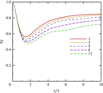
Figure 18 shows the temporal evolution of the mixedness in the mixing region. Since no perturbation exists in each
 $x{-}y$
plane initially,
 ${\it\Xi}$
starts from unity and decreases as the velocity field perturbs the mass fraction and entrains one fluid into the other, thus creating inhomogeneous regions in
 $x{-}y$
. After this transition period, the mass fraction perturbations in
 $x{-}y$
decrease. This behaviour is due to the decay in the velocity and enstrophy fields, such that the fluid newly entrained into the mixing region is not sufficiently energetic to perturb the mass fraction field. At later times, the variation in
 ${\it\Xi}$
decreases, thus suggesting a balance between molecular diffusion and entrainment from the ‘edges’ of the mixing region. With increasing density ratio, the mixedness decreases owing to the larger density and mass fraction fluctuations. On the other hand, the mixing region width increases because the heavier fluid has higher momentum (recall figure 14). These observations are consistent with the qualitative features of figures 8 and 9.
Temporal evolution of the mixedness
 ${\it\Xi}$
for
 $\mathit{Re}_{{\it\lambda},o}=100$
and different density ratios.

4. Results: dynamics of the small scales in the mixing region
We now shift our focus to the small scales. To quantify flow isotropy across the different turbulent scales in the mixing region, energy spectra are first considered in § 4.1. Then anisotropy at different length scales is investigated (§ 4.2), followed by an examination of intermittency in § 4.4. All of the quantities reported in this section are measured well within the mixing zone, in the range
 $0.25\leqslant \langle Y\rangle \leqslant 0.75$
.
4.1. Two-dimensional energy spectra
To better understand the energy distribution in the mixing region, the cumulative energy spectra, defined as
 $$\begin{eqnarray}C_{{\it\phi}}(k)=\frac{\displaystyle \int _{0}^{k}E_{{\it\phi}}(k^{\prime })\,\text{d}k^{\prime }}{\displaystyle \int _{0}^{\infty }E_{{\it\phi}}(k^{\prime })\,\text{d}k^{\prime }},\end{eqnarray}$$
are considered (Mueschke & Schilling Reference Mueschke and Schilling2009). This quantity measures how the energy is distributed between wavenumbers
 $0$
–
 $k$
, where
 $k$
is the magnitude of the two-dimensional wavevector
 $\boldsymbol{k}$
in the
 $x{-}y$
plane. At each
 $x{-}y$
plane in the mixing region, the two-dimensional energy spectra for each fluctuating field
 ${\it\phi}^{\prime }={\it\phi}-\langle {\it\phi}\rangle$
are calculated and averaged in the
 $z$
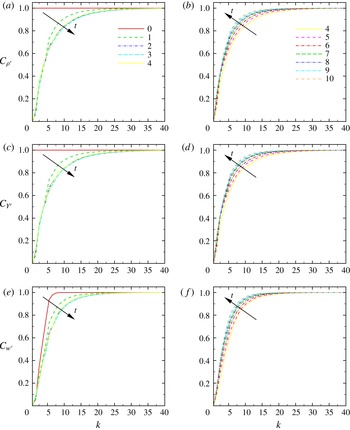
direction inside the mixing region. Figure 19 shows
 $C_{{\it\phi}}$
for the velocity, mass fraction and density fluctuating fields. Since the initial density and mass fraction fields do not contain any perturbations in the
 $x{-}y$
planes,
 $C=1$
initially for these quantities. As turbulence starts to develop from the initial random field, energy gets transferred to higher wavenumbers. After the initial transition time (up to
 $2{-}4{\it\tau}$
), the relative distribution of energy between different modes reverses as the turbulence decays.
Cumulative energy spectra of density, mass fraction, and the
 $z$
-velocity fluctuation fields at different times for
 $\mathit{Re}_{{\it\lambda},o}=100$
and
 ${\it\rho}_{2}/{\it\rho}_{1}=3$
.

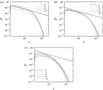
To determine the effect of the density ratio on the different scales, spectra of density, mass fraction and velocity fluctuations are shown in figure 20 for different density ratios at
 $\mathit{Re}_{{\it\lambda},o}=100$
and
 $t=5{\it\tau}$
, i.e. during self-similar growth. Increasing the density ratio does not have a significant effect on the mass fraction spectra, but yields larger energy contents at low wavenumbers in the density and
 $z$
-velocity spectra. The dependence of the
 $z$
-velocity spectra on the density ratio is attributable to varying background pressures (2.18); the larger density ratios yield higher density fluctuations across all scales at a given time.
Two-dimensional spectra of density, mass fraction and
 $z$
-velocity fluctuations for
 $\mathit{Re}_{{\it\lambda},o}=100$
,
 $t/{\it\tau}=5$
, and
 ${\it\rho}_{2}/{\it\rho}_{1}=1$
(full curve, red), 3 (dotted, orange), 5 (short dashed, blue), 8 (long dashed, purple) and 12 (dot-dashed, green). The black line corresponds to a
 $-5/3$
slope.

4.2. Temporal evolution of the Taylor and Kolmogorov scales
Perhaps the clearest indicator of anisotropy is one based on the calculation of directional length scales in the mixing region, namely Taylor and Kolmogorov scales,
 ${\it\lambda}_{i}$
and
 ${\it\eta}_{i}$
, respectively, in the
 $i$
th direction (Cook & Dimotakis Reference Cook and Dimotakis2001; Cabot & Zhou Reference Cabot and Zhou2013):
 $$\begin{eqnarray}{\it\lambda}_{i}(z,t)=\left[\frac{\langle u_{i}^{2}\rangle }{\displaystyle \left\langle \left(\frac{\partial u_{i}}{\partial x_{i}}\right)^{2}\right\rangle }\right]_{mz}^{1/2},\quad {\it\eta}_{i}(z,t)=\left[\frac{({\it\nu}/\mathit{Re})^{3}}{{\it\epsilon}_{i}}\right]_{mz}^{1/4},\end{eqnarray}$$
where
 $$\begin{eqnarray}{\it\epsilon}_{i}(z,t)=\frac{15{\it\nu}}{\mathit{Re}}\left\langle \left(\frac{\partial u_{i}}{\partial x_{i}}\right)^{2}\right\rangle\end{eqnarray}$$
is the directional dissipation rate and
 $[\boldsymbol{\cdot }]_{mz}$
is the average in the
 $z$
direction well within the mixing zone, in the range
 $0.25\leqslant \langle Y\rangle \leqslant 0.75$
. In (4.2) and (4.3), there is no sum in
 $i$
. By contrast, the overall dissipation is defined
 $$\begin{eqnarray}{\it\epsilon}=\frac{2{\it\nu}}{\mathit{Re}}\unicode[STIX]{x1D61A}_{ij}^{\ast }\unicode[STIX]{x1D61A}_{ij}^{\ast },\end{eqnarray}$$
where
 $\unicode[STIX]{x1D61A}_{ij}^{\ast }$
is defined in (3.2). Equation (4.3) is commonly used in experiments to measure dissipation as it requires measuring only one of the components of the velocity gradient tensor. This definition could raise concerns regarding the accuracy of dissipation measurements, especially in anisotropic fields (Sreenivasan & Antonia Reference Sreenivasan and Antonia1997) since (4.3) corresponds to (4.4), the exact definition of dissipation, only for spherical symmetry in incompressible homogeneous isotropic turbulence. However, this surrogacy issue is not problematic here as (4.3) is used solely to measure isotropy at the Kolmogorov scale; the full dissipation is calculated as well.
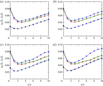
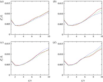
Figure 21 shows the time evolution of the directional Taylor and Kolmogorov scales. During the initial transition period (up to approximately
 $2{-}4{\it\tau}$
), the initial energy at large scales gets transferred to the small scales as discussed in the previous section. This energy transfer results in an increase in enstrophy and dissipation, and consequently a decrease in the Taylor and Kolmogorov scales. After the initial transition, the developed turbulent field decays freely, and these length scales increase with time as the smallest scales dissipate the soonest (Pope Reference Pope2000). The general trend in the evolution of the Taylor and Kolmogorov scales are in agreement with grid turbulence experiments and DNS of single-fluid decaying isotropic turbulence.
Time evolution of the directional Taylor (solid) and Kolmogorov (dashed) scales (solid) for
 $\mathit{Re}_{{\it\lambda},o}=100$
,
 ${\it\rho}_{2}/{\it\rho}_{1}=3$
(a), 5 (b), 8 (c) and 12 (d): red squares,
 $x$
component; green triangles,
 $y$
component; blue circles,
 $z$
component. The Kolmogorov scale used by measuring the full dissipation is also plotted in black.

At a modest density ratio (
 ${\it\rho}_{2}/{\it\rho}_{1}=3$
), the directional Taylor scales do not exhibit significant anisotropy. However, as the density ratio increases, the Taylor scale in the
 $z$
direction takes higher values relative to the
 $x$
and
 $y$
directions, representing anisotropy at that scale in the
 $z$
direction. This anisotropy also increases with time. As described in § 3.2, the density field evolves with the velocity during the initial transient, after which the effect of the density gradient becomes more pronounced through turbulent diffusion, as explained in § 3.3. The fact that the flow is nearly isotropic at the Taylor scale for
 ${\it\rho}_{2}/{\it\rho}_{1}=3$
is particularly important in terms of Rayleigh–Taylor turbulence as many DNS are performed at this density ratio (Cook & Dimotakis Reference Cook and Dimotakis2001; Cabot & Cook Reference Cabot and Cook2006); typically the anisotropy in the composition/density is considered as one of the main sources of anisotropy in addition to gravity in these flows. At the smallest scales, the turbulence is isotropic despite the large-scale anisotropy in density, as all three curves essentially fall onto each other. In other words, the average dissipation rate is the same in each direction, as expected for an isotropic field.
At the small scales, the growth rate of
 ${\it\eta}_{i}$
is essentially the same for all density ratios, thus suggesting that small scales are dissipated at a similar rate. This result is expected since the initial Taylor-scale Reynolds number and dissipation rate are the same across the entire field for all density ratios. The minimum achieved increases slightly with density ratio. Although both sets of length scales increase with time, the growth rate of
 ${\it\eta}_{i}$
is slightly higher than that of
 ${\it\lambda}_{x}$
and
 ${\it\lambda}_{y}$
as the density ratio is increased.
Anisotropy of the flow field can be investigated by considering the anisotropy tensor, defined as
 $$\begin{eqnarray}\unicode[STIX]{x1D609}_{ij}=\left[\frac{\langle u_{i}u_{j}\rangle }{2E}-\frac{1}{3}{\it\delta}_{ij}\right]_{mz},\end{eqnarray}$$
where
 $E$
is the turbulent kinetic energy per unit mass and
 $\langle u_{i}u_{j}\rangle$
is the
 $ij$
component of the Reynolds stress tensor. For an isotropic field,
 $\unicode[STIX]{x1D609}_{ii}=0$
since
 $\langle u^{2}\rangle =\langle v^{2}\rangle =\langle w^{2}\rangle$
. For Rayleigh–Taylor turbulence,
 $\unicode[STIX]{x1D609}_{11}\approx \unicode[STIX]{x1D609}_{22}\approx -1/6$
and
 $\unicode[STIX]{x1D609}_{33}\approx 1/3$
as
 $\langle u^{2}\rangle \approx \langle v^{2}\rangle \approx \langle w^{2}\rangle /4$
(Pope Reference Pope2000; Ramaprabhu, Karkhanis & Lawrie Reference Ramaprabhu, Karkhanis and Lawrie2013). Figure 22 shows the temporal evolution of different components of the anisotropy tensor for various density ratios. For a density ratio of 3, the three measured components of the tensor remain close to zero, corresponding to an isotropic field. As the density ratio increases,
 $\unicode[STIX]{x1D609}_{33}$
also increases, while
 $\unicode[STIX]{x1D609}_{11}$
and
 $\unicode[STIX]{x1D609}_{22}$
decrease slightly. For a density ratio of 12,
 $\unicode[STIX]{x1D609}_{33}$
reaches a high value of 0.17 at late times, representing large-scale anisotropy by the current measure. This behaviour is in agreement with the large-scale anisotropy observed for the directional Taylor microscale in the direction of the initial large-scale anisotropy.
Time evolution of the anisotropy tensor for
 $\mathit{Re}_{{\it\lambda},o}=100$
,
 ${\it\rho}_{2}/{\it\rho}_{1}=3$
(a), 5 (b), 8 (c) and 12 (d): solid, red,
 $x$
component; dashed, green,
 $y$
component; dot-dashed, blue,
 $z$
component.

After investigating the temporal evolution of the anisotropy tensor, we focus on how the velocity derivative tensor behaves across different scales at a given time. The velocity field is first coarse-grained by applying a spatial low-pass box filter over a sphere of radius
 $r$
(Tao, Katz & Meneveau Reference Tao, Katz and Meneveau2002). The enstrophy corresponding to the coarse-grained velocity is expected to scale as
 $r^{4/3}$
for
 $r$
within the inertial range (Pope Reference Pope2000). Figure 23 shows the enstrophy and the compensated enstrophy of the coarse-grained velocity at
 $t/{\it\tau}=5$
for different density ratios. The enstrophy is expected to decrease as
 $r$
increases for isotropic turbulence. This behaviour is observed for density ratios up to 8, but for the enstrophy with a density ratio of 12 exhibits non-monotone behaviour at smaller values of
 $r$
. The compensated enstrophy plots show a clear inertial range in which
 $\langle {\it\omega}_{i}{\it\omega}_{i}\rangle \sim r^{4/3}$
, for density ratios up to 5. The width of the inertial range decreases significantly for a density ratio of 8, while we do not observe any inertial range for the density ratio of 12. It is interesting to note that for small
 $r$
the coarse-grained enstrophy converges to the isotropic case (density ratio of 1) and does not exhibit significant dependence on the density ratio. As
 $r$
and density ratio increase, the coarse-grained enstrophy departs from the isotropic case. Naso & Pumir (Reference Naso and Pumir2005) reported a similar departure from the isotropic case in the context of shear flows by changing the mean shear (Naso, Pumir & Chertkov Reference Naso, Pumir and Chertkov2006; Eyink & Aluie Reference Eyink and Aluie2009).
Scaling of the coarse-grained enstrophy (a) and compensated enstrophy (b) for
 $\mathit{Re}_{{\it\lambda},o}=100$
,
 $t/{\it\tau}=5$
, and
 ${\it\rho}_{2}/{\it\rho}_{1}=1$
(squares, red), 3 (upward-pointing triangles, orange), 5 (downward-pointing triangles, blue), 8 (diamonds, purple) and 12 (circles, green).

4.3. Temporal evolution of the relevant length scales in the mass fraction field
Similar ideas can be used to examine isotropy in the mass fraction field. The directional Corrsin scale is given by (Monin & Yaglom Reference Monin and Yaglom1975; Antonia et al. Reference Antonia, Lee, Djenidi, Lavoie and Danaila2013):
 $$\begin{eqnarray}{\it\lambda}_{i}^{Y}=\left[\frac{\langle Y^{\prime 2}\rangle }{\displaystyle \left\langle \left(\frac{\partial Y^{\prime }}{\partial x_{i}}\right)^{2}\right\rangle }\right]_{mz}^{1/2},\end{eqnarray}$$
and the directional turbulent ‘scalar’ dissipation is defined as
 $$\begin{eqnarray}{\it\chi}_{i}=\left[\frac{6}{\mathit{Re}\,\mathit{Sc}}\left\langle \left(\frac{\partial Y^{\prime }}{\partial x_{i}}\right)^{2}\right\rangle \right]_{mz}.\end{eqnarray}$$
Based on dimensional arguments, the corresponding directional dissipation length scale is
 ${\it\eta}_{i}^{Y}\sim (\mathit{Re}\,\mathit{Sc})^{-3/4}{\it\chi}_{i}^{-1/4}$
. These quantities are shown in figures 24 and 25, along with the mass fraction fluctuations in figure 26. By contrast to the length scales relevant to the velocity field, the current results suggest that for a fixed density ratio the mass fraction field remains isotropic from the dissipation scale to the Corrsin scale, except small deviations at late times. Given that the Corrsin microscale represents the large-scale mass fraction fluctuations, higher values are observed as both the mass fraction fluctuations and the mixing region width are larger at higher density ratios. This phenomenon can be explained by the higher mass fraction fluctuations at higher density ratios, which lead to higher dissipation rates. The Corrsin scale is 10 times smaller than the Taylor microscale of the velocity field, which suggests that resolution requirements to resolve the Corrsin microscale accurately are much higher than those for the Taylor microscale.
Time evolution of the directional Corrsin microscale for
 $\mathit{Re}_{{\it\lambda},o}=100$
, and
 ${\it\rho}_{2}/{\it\rho}_{1}=3$
(a), 5 (b), 8 (c) and 12 (d): solid, red,
 $x$
component; dashed, green,
 $y$
component; dot-dashed, blue,
 $z$
component.

Time evolution of the directional turbulent scalar dissipation as defined in (4.7) for
 $\mathit{Re}_{{\it\lambda},o}=100$
, and
 ${\it\rho}_{2}/{\it\rho}_{1}=3$
(a), 5 (b), 8 (c) and 12 (d): solid, red,
 $x$
component; dashed, green,
 $y$
-component; dot-dashed, blue,
 $z$
component.

Average scalar fluctuation field in the
 $x{-}y$
plane at
 $t/{\it\tau}=5$
for
 $\mathit{Re}_{{\it\lambda},o}=100$
, and
 ${\it\rho}_{2}/{\it\rho}_{1}=3$
, 5, 8 and 12.

4.4. Flow intermittency
Small-scale intermittency of the velocity field is considered by measuring the directional skewness
 $S$
and kurtosis
 $K$
of the velocity derivatives in the mixing region (
 $0.25\leqslant \langle Y\rangle \leqslant 0.75$
), also measured in Tordella et al. (Reference Tordella, Iovieno and Bailey2008) and Cabot & Zhou (Reference Cabot and Zhou2013). These quantities are defined as
 $$\begin{eqnarray}S_{(\partial u_{i}/\partial x_{i})}=\left[\frac{\displaystyle \left\langle \left(\frac{\partial u_{i}}{\partial x_{i}}\right)^{3}\right\rangle }{\displaystyle \left\langle \left(\frac{\partial u_{i}}{\partial x_{i}}\right)^{2}\right\rangle ^{1.5}}\right]_{mz},\quad K_{(\partial u_{i}/\partial x_{i})}=\left[\frac{\displaystyle \left\langle \left(\frac{\partial u_{i}}{\partial x_{i}}\right)^{4}\right\rangle }{\displaystyle \left\langle \left(\frac{\partial u_{i}}{\partial x_{i}}\right)^{2}\right\rangle ^{2}}\right]_{mz},\end{eqnarray}$$
where there is no sum in
 $i$
. Despite the different density ratios, the skewness of the velocity derivatives remains at the same level (
 $S\approx -0.5$
) in all directions despite the different density ratios (figure 27), corresponding to past grid turbulence experiments (Sreenivasan & Antonia Reference Sreenivasan and Antonia1997); the same behaviour is observed in the kurtosis (figure 28) and suggests that the higher derivatives of the velocity field also remain isotropic. This result lies in contrast to level 1 mixing simulations with a jump in kinetic energy, which produce anisotropy in the skewness of the velocity derivatives (Tordella & Iovieno Reference Tordella and Iovieno2011). Results from our simulations and past studies indicate that the small-scale intermittency depends on the turbulence dynamics. Figures 27 and 28 indicates that the mass fraction field is more intermittent than the velocity field based on the higher values of the kurtosis and the higher negative value of the skewness of the mass fraction in the direction of the anisotropy. These results are consistent with grid experiments of Tong & Warhaft (Reference Tong and Warhaft1994), in which the temperature is found more intermittent than the velocity field, with a value of
 $-1.8\pm 0.2$
for the skewness of the (passive) temperature fluctuations derivative in the direction of the mean gradient.
Time evolution of skewness of the velocity derivatives (solid) and the mass fraction derivatives (dashed) for
 $\mathit{Re}_{{\it\lambda},o}=100$
and
 ${\it\rho}_{2}/{\it\rho}_{1}=3$
(a), 5 (b), 8 (c) and 12 (d); red squares,
 $x$
component; green triangles,
 $y$
component; blue circles,
 $z$
component.

Time evolution of kurtosis of the velocity derivatives (solid) and the mass fraction derivatives (dashed) for
 $\mathit{Re}_{{\it\lambda},o}=100$
and
 ${\it\rho}_{2}/{\it\rho}_{1}=3$
(a), 5 (b), 8 (c) and 12 (d): red squares,
 $x$
component; green triangles,
 $y$
component; blue circles,
 $z$
component.

5. Conclusions
DNS is conducted using a novel set-up to investigate level 2 turbulent mixing, with a focus on anisotropy generated solely by a density gradient. The velocity is initialised by a random solenoidal field that produces homogeneous isotropic turbulence with zero mean velocity, which is then left to decay freely in the absence of kinetic energy production mechanisms, e.g. shear in the Kelvin–Helmholtz instability or gravity in the Rayleigh–Taylor instability. Superposed onto this velocity field, an unperturbed interface initially separates a heavy fluid from a light one. The fluid properties are selected such that the kinematic viscosity, and thus the dissipation rate, is the same in both fluids despite their different densities. The rationale behind this strategy is that conventional turbulence scalings are based on kinetic energy per unit mass and kinematic viscosity, such that density and dynamic viscosity do not appear. Thus, by matching the initial kinematics (root-mean-square velocity) and the corresponding dissipation (kinematic viscosity) in the two fluids, the turbulence decays at the same rate in the two fluids, even though there is an initial gradient in the kinetic energy (per unit volume). Since, the mean kinetic energy per unit mass is the same in each fluid, anisotropy initially lies in the density gradient only. Thus, anisotropy observed at later times can be attributed to this gradient, such that the effect of large-scale density differences on the turbulence can be considered, independently from any other contribution. As the flow evolves, mixing occurs between the heavy and light fluids. We explore how the mixing region grows for different density ratios and Reynolds numbers and examine both the large- and small-scale dynamics. From this study, we can make the following key conclusions.
-
(i) As the initial random field evolves to a turbulent state, energy gets transferred to higher wavenumbers. Over approximately the first two to four eddy turnover times, the dynamics exhibit little dependence on the density ratio. After this initial transient and once decay becomes important, the distribution of energy reverses as the small scales dissipate faster.
-
(ii) After the initial transient, the mixing region grows self-similarly through a process that can be described by turbulence diffusion. Several theoretical arguments are proposed to describe how the mixing region width scales with time, in agreement with the simulations results and past work. For higher density ratios, it takes a longer time to achieve self-similar growth. The observed time exponent for the growth of the mixing region in this study is close to those reported in studies of turbulent mixing following the Richtmyer–Meshkov instability after reshock (Tritschler et al. Reference Tritschler, Olson, Lele, Hickel, Hu and Adams2014). This observation is expected, since the turbulence produced by such flows is very similar to that in the present study.
-
(iii) Bubbles and spikes grow in an asymmetric fashion due to the higher momentum of heavier eddies in the mixing region. As a result, the mid-plane corresponding to
$\langle Y\rangle =0.5$
shifts toward the lighter fluid as the density ratio is increased. This observation is important in the context of the Rayleigh–Taylor instability, as the temporal evolution of turbulence statistics is often reported at the
$z=0$
plane. -
(iv) While a wider mixing region is achieved at higher density ratios, the flow is found to be less molecularly mixed therein.
-
(v) At the Taylor scale, the turbulence remains almost isotropic at modest density ratios (
${\it\rho}_{2}/{\it\rho}_{1}=1$
and 3), while it becomes clearly anisotropic at higher density ratios (
${\it\rho}_{2}/{\it\rho}_{1}=8$
, and 12). The fact that the flow is almost isotropic at the Taylor scale for
${\it\rho}_{2}/{\it\rho}_{1}=3$
is particularly important in terms of Rayleigh–Taylor turbulence, as many past DNS have been performed at this density ratio (Cook & Dimotakis Reference Cook and Dimotakis2001; Cabot & Cook Reference Cabot and Cook2006); typically the anisotropy in the composition is also considered as one of the main sources of anisotropy in addition to gravity in these flows. The scalar field appears to remains almost isotropic up to the Corrsin scale, even for high density ratios. -
(vi) Flow intermittency is investigated by measuring the skewness and kurtosis of the velocity and the scalar derivatives in different directions. The intermittency of the velocity field remains the same in different directions and takes values corresponding to grid turbulence. The scalar field is more intermittent than the velocity and exhibits larger intermittency in the direction of the scalar gradient, in agreement with past grid-turbulence experiments.


This paper constitutes the first in a series on level 2 turbulent mixing and lays the foundations for understanding how density gradients lead to anisotropy. Our next study will focus on the combined effect of a gravitational field with a density gradient, specifically in the context of Rayleigh–Taylor turbulence.
Acknowledgements
The authors gratefully acknowledge helpful discussions with Professor D. Dowling. This research was supported in part by the DOE NNSA/ASC under the Predictive Science Academic Alliance Program by grant no. DEFC5208NA28616. This work used resources from the Extreme Science and Engineering Discovery Environment (XSEDE), which is supported by National Science Foundation grant number OCI-1053575.