1 Introduction
The air–sea exchange of scalar quantities, such as water vapour and heat, near the air–water interface plays a vital role in global and regional air–sea interactions (Smith Reference Smith1988; DeCosmo et al. Reference DeCosmo, Katsaros, Smith, Anderson, Oost, Bumke and Chadwick1996; Fairall et al. Reference Fairall, Bradley, Rogers, Edson and Young1996; Edson et al. Reference Edson, Crawford, Crescenti, Farrar, Frew, Gerbi, Helmis, Hristov, Khelif and Jessup2007). Turbulent transport of scalars in the air above the sea surface is strongly affected by the surface waves. The periodical surface curvatures and the motions of these waves can induce considerable disturbance to the air turbulent flows near the wave surface, affecting the transport of both momentum and scalars (Edson et al. Reference Edson, Crawford, Crescenti, Farrar, Frew, Gerbi, Helmis, Hristov, Khelif and Jessup2007; Sullivan & McWilliams Reference Sullivan and McWilliams2010).
Various experimental studies have been conducted in the past several decades to characterize the effect of sea-surface waves on air–sea scalar transport. For example, Fairall et al. (Reference Fairall, Bradley, Rogers, Edson and Young1996), Bourassa, Vincent & Wood (Reference Bourassa, Vincent and Wood1999) and Edson et al. (Reference Edson, Zappa, Ware, McGillis and Hare2004) measured the bulk properties of the air–sea scalar exchange, and parameterized the scalar flux profiles in terms of averaged air–sea interfacial properties such as the scalar transfer coefficient, sea-surface scalar roughness length, and convective scaling velocity. Edson et al. (Reference Edson, Crawford, Crescenti, Farrar, Frew, Gerbi, Helmis, Hristov, Khelif and Jessup2007) measured the velocity, temperature and relative humidity in the marine atmospheric boundary layer (ABL) under low winds in the CBLAST-LOW experiment. Based on the CBLAST-LOW data, Katsouvas, Helmis & Wang (Reference Katsouvas, Helmis and Wang2007) performed quadrant analysis for the scalar and momentum fluxes. Katul, Sempreviva & Cava (Reference Katul, Sempreviva and Cava2008) analyzed the data from RASEX (Risø Air Sea EXperiment) and developed a one-dimensional model for the temperature–humidity covariance. Experimental studies of air–sea scalar transport have provided valuable insights and parameterizations for modelling air–sea interactions.
In recent years, enabled by the continuous advancement of computer power, numerical simulation has become a valuable tool for studying the fine-scale scalar transport phenomena near the air–water interface. Modelling the air turbulence over sea surfaces is challenging, primarily due to the difficulty associated with modelling the effect of sea-surface waves. One approach is to approximate the marine ABL as turbulence over a flat surface, with the wave effect parameterized as the sea-surface roughness length (e.g. Charnock Reference Charnock1955; Fairall et al.
Reference Fairall, Bradley, Rogers, Edson and Young1996). However, accurately parameterizing the sea-surface roughness is found to be quite challenging due to the complexity in wind–wave interaction (e.g. Donelan Reference Donelan, LeMehaute and Hanes1990; Toba, Smith & Ebuchi Reference Toba, Smith, Ebuchi, Jones and Toba2001; Yang, Meneveau & Shen Reference Yang, Meneveau and Shen2013). Instead, many previous numerical studies attempted to directly simulate air turbulence over progressive surface waves, with the instantaneous wave motions imposed in the simulation as bottom boundary conditions (e.g. Sullivan, McWilliams & Moeng Reference Sullivan, McWilliams and Moeng2000; Sullivan & McWilliams Reference Sullivan and McWilliams2002; Kihara et al.
Reference Kihara, Hanazaki, Mizuya and Ueda2007; Yang & Shen Reference Yang and Shen2009, Reference Yang and Shen2010; Druzhinin, Troitskayaa & Zilitinkevich Reference Druzhinin, Troitskayaa and Zilitinkevich2016). Most of these previous studies focused on the momentum transfer between the air turbulence and the water waves. Sullivan & McWilliams (Reference Sullivan and McWilliams2002) and Druzhinin et al. (Reference Druzhinin, Troitskayaa and Zilitinkevich2016) considered the temperature field in their simulations with a Prandtl number of
 $0.7$
, corresponding to the ratio of kinematic viscosity to thermal diffusivity of the air, and studied the effects of various stratification conditions (characterized by the Richardson number) on the characteristics of the air turbulence. On the other hand, a number of numerical studies have been performed focusing on the statistics of scalar fluctuations over stationary wavy walls (e.g. Antonia & Kim Reference Antonia and Kim1991; Kawamura et al.
Reference Kawamura, Ohsaka, Abe and Yamamoto1998; Dellil, Azzi & Jubran Reference Dellil, Azzi and Jubran2004; Park, Choi & Suzuki Reference Park, Choi and Suzuki2004; Choi & Suzuki Reference Choi and Suzuki2005; Rossi Reference Rossi2010). These studies have shown significant effects of the stationary waves on the characteristics of scalar transport, such as the surface scalar flux, the mean scalar concentration, the scalar variance and the turbulent scalar fluxes. However, there is still a lack of studies devoted to the mechanism of scalar transport in turbulence over progressive surface waves, which is expected to be significantly different from the cases with stationary wavy walls (Belcher & Hunt Reference Belcher and Hunt1998; Sullivan & McWilliams Reference Sullivan and McWilliams2010).
In this study, the direct numerical simulation (DNS) solver developed by Yang & Shen (Reference Yang and Shen2011a
) is adopted, which uses a boundary-fitted computational grid system that follows the instantaneous wave surface elevation and motions, allowing one to resolve the details of the turbulent flow above and in the vicinity of the mobile wave surface. In the present study, this DNS solver is further expanded by including a scalar transport solver within the boundary-fitted spatial discretization framework, and is used to simulate the transport of passive scalars in turbulent flows over progressive surface waves. As in many recent numerical studies, a plane progressive surface wave train is imposed at the bottom of the simulation domain (e.g. Sullivan et al.
Reference Sullivan, McWilliams and Moeng2000, Reference Sullivan, Edson, Hristov and McWilliams2008; Sullivan & McWilliams Reference Sullivan and McWilliams2002; Kihara et al.
Reference Kihara, Hanazaki, Mizuya and Ueda2007; Yang & Shen Reference Yang and Shen2009, Reference Yang and Shen2010; Hara & Sullivan Reference Hara and Sullivan2015; Druzhinin et al.
Reference Druzhinin, Troitskayaa and Zilitinkevich2016). A relatively large wave steepness of
 $ak=0.25$
is considered, where
 $a$
is the wave amplitude and
 $k$
is the wavenumber. To account for the nonlinearity associated with such a steep wave, a high-order Stokes wave solution is used to prescribe the wave surface elevation and orbital velocity. Three representative wave-to-wind speed ratios
 $c/u_{\ast }$
(also called the wave age) are considered, including
 $c/u_{\ast }=2$
(slow waves),
 $14$
(intermediate waves) and
 $25$
(fast waves), where
 $c$
is the wave phase speed and
 $u_{\ast }$
is the friction velocity of the turbulence. In order to achieve the desired value for
 $c/u_{\ast }$
, the turbulent flow is driven by a constant streamwise stress applied at the top flat boundary, and the mean flow has a Couette-flow-type of velocity profile, but with the mean velocity at the top boundary varying for different wave conditions. The scalar transport is known to be largely affected by the Schmidt number
 $Sc=\unicode[STIX]{x1D708}/D$
, where
 $\unicode[STIX]{x1D708}$
is the kinematic viscosity and
 $D$
is the scalar molecular diffusivity. For each wave condition, four Schmidt numbers are considered, including
 $Sc=0.5$
,
 $1.0$
,
 $2.0$
and
 $4.0$
. Based on the DNS data, the effects of surface waves on the scalar transport are studied by various statistical analysis techniques, including time and plane average, wave phase average, quadrant analysis and conditional average. The correlations between coherent vortical structures and turbulent scalar transport events are also studied by direct observation of instantaneous snapshots and quadrant-based conditional averages.
The remainder of this paper is organized as follows. First, the mathematical formulas and numerical schemes of the DNS solver are described in § 2. Then the configurations of the simulation cases are given in § 3, together with some sample results of the DNS. In § 4, various types of statistical analyses of the DNS data are performed, and the effects of surface waves on the characteristics of flow structures and turbulent scalar transport are discussed. Finally, conclusions are given in § 5.
2 Description of DNS
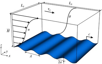
As shown in figure 1, this study uses DNS to examine the transport of passive scalars in a three-dimensional stress-driven turbulent Couette flow over a plane progressive surface wave train. The Cartesian coordinates are denoted as
 $x_{i}(i=1,2,3)=(x,y,z)$
, where
 $x$
and
 $y$
are the horizontal coordinates and
 $z$
is the vertical coordinate, with
 $z=0$
being the mean elevation of the surface wave at the bottom of the simulation domain;
 $u_{i}(i=1,2,3)=(u,v,w)$
are the corresponding velocity components in
 $x$
-,
 $y$
- and
 $z$
-directions, respectively.
In the simulation, the flow is driven by a constant streamwise shear stress
 $\unicode[STIX]{x1D70F}_{x}$
prescribed on the rigid flat top boundary, which prescribes a fixed turbulence friction velocity of
 $u_{\ast }=\sqrt{\unicode[STIX]{x1D70F}_{x}/\unicode[STIX]{x1D70C}}$
, where
 $\unicode[STIX]{x1D70C}$
is the fluid density. The bottom of the flow is bounded and distorted by a two-dimensional wave train that propagates in the
 $x$
-direction. This stress-driven Couette flow configuration has been used as a canonical problem to study the surface water wave effect on turbulent air flows in many previous numerical studies (e.g. Gent & Taylor Reference Gent and Taylor1976; Li, Xu & Taylor Reference Li, Xu and Taylor2000; Kihara et al.
Reference Kihara, Hanazaki, Mizuya and Ueda2007; Yang & Shen Reference Yang and Shen2009, Reference Yang and Shen2010). A passive scalar
 $\unicode[STIX]{x1D703}$
is transported by the turbulent flow, with a Dirichlet boundary condition of
 $\unicode[STIX]{x1D703}=0$
on the bottom wave surface and
 $\unicode[STIX]{x1D703}=2$
on the top boundary. This configuration for
 $\unicode[STIX]{x1D703}$
results in
 $\unicode[STIX]{x1D703}\approx 1$
at the centre of the simulation domain. We remark that in this canonical simulation configuration, we set the passive scalar to have a smaller value near the wave surface and a larger value near the upper boundary, similar to many previous numerical studies (e.g. Dellil et al.
Reference Dellil, Azzi and Jubran2004; Park et al.
Reference Park, Choi and Suzuki2004; Rossi Reference Rossi2010). In some applications, e.g. the moisture in the marine atmospheric boundary layer, the scalars have higher concentrations near the wave surface. Because
 $\unicode[STIX]{x1D703}$
is assumed to be passive and its governing equation is linear with respect to
 $\unicode[STIX]{x1D703}$
, the results reported in this study can be converted to the reversed configuration with a larger scalar value near the wave surface. We choose the current configuration as it allows us to compare the current DNS results to the previously reported results of passive scalar transport in turbulent boundary layers over flat and wavy boundaries.
Sketch of the simulation configuration. A three-dimensional turbulent Couette flow is driven by a constant shear stress
 $\unicode[STIX]{x1D70F}_{x}$
applied at the top boundary, and flows over a plane progressive surface wave train. The surface wave has a wavelength
 $\unicode[STIX]{x1D706}$
and an amplitude
 $a$
. The wave propagates in the
 $x$
-direction with a phase speed
 $c$
. The passive scalar field
 $\unicode[STIX]{x1D703}$
is transported by the turbulent Couette flow, with Dirichlet boundary conditions of
 $\unicode[STIX]{x1D703}=0$
and
 $\unicode[STIX]{x1D703}=2$
at the bottom and top boundaries, respectively.

In the DNS, the turbulent carrier flow is described by the three-dimensional incompressible Navier–Stokes equations
 $$\begin{eqnarray}\displaystyle & \displaystyle \frac{\unicode[STIX]{x2202}u_{i}}{\unicode[STIX]{x2202}x_{i}}=0, & \displaystyle\end{eqnarray}$$
 $$\begin{eqnarray}\displaystyle & \displaystyle \frac{\unicode[STIX]{x2202}u_{i}}{\unicode[STIX]{x2202}t}+\frac{\unicode[STIX]{x2202}(u_{i}u_{j})}{\unicode[STIX]{x2202}x_{j}}=-\frac{1}{\unicode[STIX]{x1D70C}}\frac{\unicode[STIX]{x2202}p}{\unicode[STIX]{x2202}x_{i}}+\unicode[STIX]{x1D708}\frac{\unicode[STIX]{x2202}^{2}u_{i}}{\unicode[STIX]{x2202}x_{j}\unicode[STIX]{x2202}x_{j}}, & \displaystyle\end{eqnarray}$$
where
 $p$
is the pressure. The transport of the passive scalar
 $\unicode[STIX]{x1D703}(x,y,z,t)$
is governed by a convection–diffusion equation
 $$\begin{eqnarray}\frac{\unicode[STIX]{x2202}\unicode[STIX]{x1D703}}{\unicode[STIX]{x2202}t}+\frac{\unicode[STIX]{x2202}(\unicode[STIX]{x1D703}u_{j})}{\unicode[STIX]{x2202}x_{j}}=D\frac{\unicode[STIX]{x2202}^{2}\unicode[STIX]{x1D703}}{\unicode[STIX]{x2202}x_{j}\unicode[STIX]{x2202}x_{j}}.\end{eqnarray}$$
The effect of progressive surface waves on the turbulence is imposed through a Dirichlet velocity boundary condition at the bottom wave surface,
 $u_{i}(z=\unicode[STIX]{x1D702})=(u_{s},v_{s},w_{s})$
, where
 $\unicode[STIX]{x1D702}$
is the wave surface elevation and
 $(u_{s},v_{s},w_{s})$
are the wave surface orbital velocities. In this study, we use a high-order two-dimensional Stokes wave solution to prescribe the motions of the plane-progressive surface wave train (Stokes Reference Stokes1847),
 $$\begin{eqnarray}\displaystyle & \displaystyle \unicode[STIX]{x1D702}(x,y,t)=\mathop{\sum }_{n=1}^{N}(ak)^{n-1}\unicode[STIX]{x1D702}^{(n)}(x,y,t), & \displaystyle\end{eqnarray}$$
 $$\begin{eqnarray}\displaystyle & \displaystyle u_{s}(x,y,t)=\mathop{\sum }_{n=1}^{N}(ak)^{n-1}u_{s}^{(n)}(x,y,t), & \displaystyle\end{eqnarray}$$
 $$\begin{eqnarray}\displaystyle & \displaystyle v_{s}(x,y,t)=0, & \displaystyle\end{eqnarray}$$
 $$\begin{eqnarray}\displaystyle & \displaystyle w_{s}(x,y,t)=\mathop{\sum }_{n=1}^{N}(ak)^{n-1}w_{s}^{(n)}(x,y,t), & \displaystyle\end{eqnarray}$$
where the variables with superscript ‘
 $(n)$
’ indicate the
 $n$
th mode of the corresponding wave quantity. In particular, following Dommermuth & Yue (Reference Dommermuth and Yue1987), we directly solve the nonlinear equations associated with the mapping function in Schwartz (Reference Schwartz1974) by using Newton iteration up to a high order of
 $N=192$
. As a reference, the Stokes solution up to the second order can be found in Dean & Dalrymple (Reference Dean and Dalrymple1991). For the purpose of defining some key parameters of the wave boundary conditions, in the following equations only the leading order mode of the Stokes wave solution is given, which is the same as the Airy wave solution and has been used in many prior DNS studies (e.g. Sullivan et al.
Reference Sullivan, McWilliams and Moeng2000, Reference Sullivan, Edson, Hristov and McWilliams2008; Kihara et al.
Reference Kihara, Hanazaki, Mizuya and Ueda2007; Hara & Sullivan Reference Hara and Sullivan2015; Druzhinin et al.
Reference Druzhinin, Troitskayaa and Zilitinkevich2016):
 $$\begin{eqnarray}\displaystyle & \displaystyle \unicode[STIX]{x1D702}^{(1)}(x,y,t)=a\sin \,k(x-ct), & \displaystyle\end{eqnarray}$$
 $$\begin{eqnarray}\displaystyle & \displaystyle u_{s}^{(1)}(x,y,t)=akc\,\sin k(x-ct), & \displaystyle\end{eqnarray}$$
 $$\begin{eqnarray}\displaystyle & \displaystyle v_{s}^{(1)}(x,y,t)=0, & \displaystyle\end{eqnarray}$$
 $$\begin{eqnarray}\displaystyle & \displaystyle w_{s}^{(1)}(x,y,t)=akc\,\cos k(x-ct). & \displaystyle\end{eqnarray}$$
Here,
 $a$
is the amplitude of the leading wave mode,
 $k=2\unicode[STIX]{x03C0}/\unicode[STIX]{x1D706}$
is its wavenumber,
 $\unicode[STIX]{x1D706}$
is its wavelength, and
 $c$
is its phase speed.
We note that the current DNS solver can be dynamically coupled with another solver for the water waves, allowing the simulation of turbulence with a dynamically evolving wave field (Yang & Shen Reference Yang and Shen2011b ). Because this study focuses on understanding the fundamental mechanisms of the surface wave effects on the passive scalar transport, we choose to use the canonical configuration with a prescribed Stokes wave boundary condition, which allows for a precise phase average based on the periodic wave form and yields well-converged statistics for the flow and scalar fields. Moreover, when a more realistic dynamically evolving wave field (either monochromatic or broadband) is considered, a realistically high Reynolds number should be considered in order to capture the interaction between turbulence and surface waves over a wide range of scales, for which the flow and scalar fields have to be simulated using wall-modelled large-eddy simulation (Yang et al. Reference Yang, Meneveau and Shen2013; Yang, Meneveau & Shen Reference Yang, Meneveau and Shen2014a ,Reference Yang, Meneveau and Shen b ). These more realistic and complicated conditions go beyond the scope of the current canonical study, but are worth considering in future studies of scalar transport in turbulent wind over ocean waves.
To capture the surface wave effect on the scalar field, the DNS solver uses a boundary-fitted coordinate system that follows the instantaneous deformation of the wave surface. The irregular wave surface-bounded domain in the physical space
 $(x,y,z,t)$
is transformed to a right rectangular prism in the computational space
 $(\unicode[STIX]{x1D709},\unicode[STIX]{x1D713},\unicode[STIX]{x1D701},\unicode[STIX]{x1D70F})$
with the following algebraic mapping:
 $$\begin{eqnarray}\unicode[STIX]{x1D709}=x,\quad \unicode[STIX]{x1D713}=y,\quad \unicode[STIX]{x1D701}=\frac{z-\unicode[STIX]{x1D702}(x,y,t)}{H(x,y,t)}=\frac{z-\unicode[STIX]{x1D702}(x,y,t)}{\overline{H}-\unicode[STIX]{x1D702}(x,y,t)},\quad \unicode[STIX]{x1D70F}=t.\end{eqnarray}$$
Here, the height of the physical domain,
 $H(x,y,t)$
, is decomposed into an average height
 $\overline{H}$
and a wave induced variation
 $-\unicode[STIX]{x1D702}(x,y,t)$
. Similar to
 $x_{i}$
, the spatial coordinates in the computational space can also be denoted using the index notation as
 $\unicode[STIX]{x1D709}_{i}(i=1,2,3)=(\unicode[STIX]{x1D709},\unicode[STIX]{x1D713},\unicode[STIX]{x1D701})$
.
The Jacobian matrix of the spatial coordinate transformation is
 $$\begin{eqnarray}\unicode[STIX]{x1D645}=\left[\begin{array}{@{}ccc@{}}\displaystyle \frac{\unicode[STIX]{x2202}\unicode[STIX]{x1D709}}{\unicode[STIX]{x2202}x} & \displaystyle \frac{\unicode[STIX]{x2202}\unicode[STIX]{x1D709}}{\unicode[STIX]{x2202}y} & \displaystyle \frac{\unicode[STIX]{x2202}\unicode[STIX]{x1D709}}{\unicode[STIX]{x2202}z}\\ \displaystyle \frac{\unicode[STIX]{x2202}\unicode[STIX]{x1D713}}{\unicode[STIX]{x2202}x} & \displaystyle \frac{\unicode[STIX]{x2202}\unicode[STIX]{x1D713}}{\unicode[STIX]{x2202}y} & \displaystyle \frac{\unicode[STIX]{x2202}\unicode[STIX]{x1D713}}{\unicode[STIX]{x2202}z}\\ \displaystyle \frac{\unicode[STIX]{x2202}\unicode[STIX]{x1D701}}{\unicode[STIX]{x2202}x} & \displaystyle \frac{\unicode[STIX]{x2202}\unicode[STIX]{x1D701}}{\unicode[STIX]{x2202}y} & \displaystyle \frac{\unicode[STIX]{x2202}\unicode[STIX]{x1D701}}{\unicode[STIX]{x2202}z}\end{array}\right]=\left[\begin{array}{@{}ccc@{}}1 & 0 & 0\\ 0 & 1 & 0\\ \displaystyle \frac{\unicode[STIX]{x1D701}-1}{\overline{H}-\unicode[STIX]{x1D702}}\frac{\unicode[STIX]{x2202}\unicode[STIX]{x1D702}}{\unicode[STIX]{x2202}x} & \displaystyle \frac{\unicode[STIX]{x1D701}-1}{\overline{H}-\unicode[STIX]{x1D702}}\frac{\unicode[STIX]{x2202}\unicode[STIX]{x1D702}}{\unicode[STIX]{x2202}y} & \displaystyle \frac{1}{\overline{H}-\unicode[STIX]{x1D702}}\end{array}\right].\end{eqnarray}$$
Because the wave surface oscillates in time, a transformation is also required for the temporal derivative terms, i.e.
 $$\begin{eqnarray}\frac{\unicode[STIX]{x2202}}{\unicode[STIX]{x2202}t}=\frac{\unicode[STIX]{x2202}}{\unicode[STIX]{x2202}\unicode[STIX]{x1D70F}}+\frac{\unicode[STIX]{x2202}\unicode[STIX]{x1D701}}{\unicode[STIX]{x2202}t}\frac{\unicode[STIX]{x2202}}{\unicode[STIX]{x2202}\unicode[STIX]{x1D701}},\quad \text{where}~\frac{\unicode[STIX]{x2202}\unicode[STIX]{x1D701}}{\unicode[STIX]{x2202}t}=\frac{\unicode[STIX]{x1D701}-1}{\overline{H}-\unicode[STIX]{x1D702}}\frac{\unicode[STIX]{x2202}\unicode[STIX]{x1D702}}{\unicode[STIX]{x2202}t}.\end{eqnarray}$$
By applying the chain rule together with (2.13) and (2.14), we write the governing equations (2.1)–(2.3) in the wave-surface-fitted coordinates as
 $$\begin{eqnarray}\displaystyle & \displaystyle \unicode[STIX]{x1D611}_{kj}\frac{\unicode[STIX]{x2202}u_{j}}{\unicode[STIX]{x2202}\unicode[STIX]{x1D709}_{k}}=0, & \displaystyle\end{eqnarray}$$
 $$\begin{eqnarray}\displaystyle & \displaystyle \frac{\unicode[STIX]{x2202}u_{i}}{\unicode[STIX]{x2202}\unicode[STIX]{x1D70F}}+\unicode[STIX]{x1D6FF}_{j3}\frac{\unicode[STIX]{x2202}\unicode[STIX]{x1D701}}{\unicode[STIX]{x2202}t}\frac{\unicode[STIX]{x2202}u_{i}}{\unicode[STIX]{x2202}\unicode[STIX]{x1D709}_{j}}+\unicode[STIX]{x1D611}_{kj}\frac{\unicode[STIX]{x2202}(u_{i}u_{j})}{\unicode[STIX]{x2202}\unicode[STIX]{x1D709}_{k}}=-\frac{\unicode[STIX]{x1D611}_{ki}}{\unicode[STIX]{x1D70C}}\frac{\unicode[STIX]{x2202}p}{\unicode[STIX]{x2202}\unicode[STIX]{x1D709}_{k}}+\unicode[STIX]{x1D708}\unicode[STIX]{x1D611}_{nj}\frac{\unicode[STIX]{x2202}}{\unicode[STIX]{x2202}\unicode[STIX]{x1D709}_{n}}\!\!\left(\unicode[STIX]{x1D611}_{kj}\frac{\unicode[STIX]{x2202}u_{i}}{\unicode[STIX]{x2202}\unicode[STIX]{x1D709}_{k}}\right), & \displaystyle\end{eqnarray}$$
 $$\begin{eqnarray}\displaystyle & \displaystyle \frac{\unicode[STIX]{x2202}\unicode[STIX]{x1D703}}{\unicode[STIX]{x2202}\unicode[STIX]{x1D70F}}+\unicode[STIX]{x1D6FF}_{j3}\frac{\unicode[STIX]{x2202}\unicode[STIX]{x1D701}}{\unicode[STIX]{x2202}t}\frac{\unicode[STIX]{x2202}\unicode[STIX]{x1D703}}{\unicode[STIX]{x2202}\unicode[STIX]{x1D709}_{j}}+\unicode[STIX]{x1D611}_{kj}\frac{\unicode[STIX]{x2202}(\unicode[STIX]{x1D703}u_{j})}{\unicode[STIX]{x2202}\unicode[STIX]{x1D709}_{k}}=D\unicode[STIX]{x1D611}_{nj}\frac{\unicode[STIX]{x2202}}{\unicode[STIX]{x2202}\unicode[STIX]{x1D709}_{n}}\!\!\left(\unicode[STIX]{x1D611}_{kj}\frac{\unicode[STIX]{x2202}\unicode[STIX]{x1D703}}{\unicode[STIX]{x2202}\unicode[STIX]{x1D709}_{k}}\right), & \displaystyle\end{eqnarray}$$
where
 $\unicode[STIX]{x1D611}_{ij}$
is the index notation of the matrix
 $\unicode[STIX]{x1D645}$
and
 $\unicode[STIX]{x1D6FF}_{ij}$
is the Kronecker delta. Note that
 $u_{i}$
are the velocities in the physical space.
In DNS, equations (2.15)–(2.17) are discretized in the computational space
 $(\unicode[STIX]{x1D709},\unicode[STIX]{x1D713},\unicode[STIX]{x1D701},\unicode[STIX]{x1D70F})$
and solved numerically. In particular, a Fourier-series-based pseudo-spectral method is used in the
 $(\unicode[STIX]{x1D709},\unicode[STIX]{x1D713})$
-plane, with evenly spaced collocated grid points in both directions. The standard
 $2/3$
-rule is used for eliminating the aliasing error. In the vertical direction, a second-order finite-difference method is used based on a staggered
 $\unicode[STIX]{x1D701}$
-grid. The vertical grid is clustered near the top boundary and the bottom wave surface to provide adequate resolution for the boundary layers. The governing equations are integrated in time with a fractional-step method. For both (2.16) and (2.17), the nonlinear convection terms are advanced in time using a second-order Adams–Bashforth scheme. In order to resolve the boundary layer without requiring a significantly small timestep, a semi-implicit scheme is desired for time advancement of the viscous diffusion terms in (2.16) and (2.17). Due to the coordinate transformation (2.12), in the computational space the Laplacian operator in the diffusion terms becomes
 $$\begin{eqnarray}\displaystyle \unicode[STIX]{x1D6FB}^{2} & = & \displaystyle \unicode[STIX]{x1D611}_{nj}\frac{\unicode[STIX]{x2202}}{\unicode[STIX]{x2202}\unicode[STIX]{x1D709}_{n}}\left(\unicode[STIX]{x1D611}_{kj}\frac{\unicode[STIX]{x2202}}{\unicode[STIX]{x2202}\unicode[STIX]{x1D709}_{k}}\right)=\underbrace{\frac{\unicode[STIX]{x2202}^{2}}{\unicode[STIX]{x2202}\unicode[STIX]{x1D709}^{2}}+\frac{\unicode[STIX]{x2202}^{2}}{\unicode[STIX]{x2202}\unicode[STIX]{x1D713}^{2}}+2\unicode[STIX]{x1D611}_{31}\frac{\unicode[STIX]{x2202}^{2}}{\unicode[STIX]{x2202}\unicode[STIX]{x1D709}\unicode[STIX]{x2202}\unicode[STIX]{x1D701}}+2\unicode[STIX]{x1D611}_{32}\frac{\unicode[STIX]{x2202}^{2}}{\unicode[STIX]{x2202}\unicode[STIX]{x1D713}\unicode[STIX]{x2202}\unicode[STIX]{x1D701}}}_{\displaystyle \unicode[STIX]{x1D6FB}_{\unicode[STIX]{x1D709}\unicode[STIX]{x1D713}}^{2}}\nonumber\\ \displaystyle & & \displaystyle +\,\underbrace{\left(\unicode[STIX]{x1D611}_{31}^{2}+\unicode[STIX]{x1D611}_{32}^{2}+\unicode[STIX]{x1D611}_{33}^{2}\right)\frac{\unicode[STIX]{x2202}^{2}}{\unicode[STIX]{x2202}\unicode[STIX]{x1D701}^{2}}+\left(\frac{\unicode[STIX]{x2202}^{2}\unicode[STIX]{x1D701}}{\unicode[STIX]{x2202}x^{2}}+\frac{\unicode[STIX]{x2202}^{2}\unicode[STIX]{x1D701}}{\unicode[STIX]{x2202}y^{2}}\right)\frac{\unicode[STIX]{x2202}}{\unicode[STIX]{x2202}\unicode[STIX]{x1D701}}}_{\displaystyle \unicode[STIX]{x1D6FB}_{\unicode[STIX]{x1D701}}^{2}},\end{eqnarray}$$
where
 $$\begin{eqnarray}\displaystyle & \displaystyle \frac{\unicode[STIX]{x2202}^{2}\unicode[STIX]{x1D701}}{\unicode[STIX]{x2202}x^{2}}=\frac{\unicode[STIX]{x1D701}-1}{\overline{H}-\unicode[STIX]{x1D702}}\frac{\unicode[STIX]{x2202}^{2}\unicode[STIX]{x1D702}}{\unicode[STIX]{x2202}x^{2}}+\frac{2(\unicode[STIX]{x1D701}-1)}{(\overline{H}-\unicode[STIX]{x1D702})^{2}}\left(\frac{\unicode[STIX]{x2202}\unicode[STIX]{x1D702}}{\unicode[STIX]{x2202}x}\right)^{2}, & \displaystyle\end{eqnarray}$$
 $$\begin{eqnarray}\displaystyle & \displaystyle \frac{\unicode[STIX]{x2202}^{2}\unicode[STIX]{x1D701}}{\unicode[STIX]{x2202}y^{2}}=\frac{\unicode[STIX]{x1D701}-1}{\overline{H}-\unicode[STIX]{x1D702}}\frac{\unicode[STIX]{x2202}^{2}\unicode[STIX]{x1D702}}{\unicode[STIX]{x2202}y^{2}}+\frac{2(\unicode[STIX]{x1D701}-1)}{(\overline{H}-\unicode[STIX]{x1D702})^{2}}\left(\frac{\unicode[STIX]{x2202}\unicode[STIX]{x1D702}}{\unicode[STIX]{x2202}y}\right)^{2}. & \displaystyle\end{eqnarray}$$
In the Laplacian operator (2.18), the first part,
 $\unicode[STIX]{x1D6FB}_{\unicode[STIX]{x1D709}\unicode[STIX]{x1D713}}^{2}$
, involves derivatives with respect to
 $\unicode[STIX]{x1D709}$
and
 $\unicode[STIX]{x1D713}$
, and is thus treated with the second-order Adams–Bashforth scheme; the second part,
 $\unicode[STIX]{x1D6FB}_{\unicode[STIX]{x1D701}}^{2}$
, is treated semi-implicitly using the Crank–Nicolson scheme. Note that if the Crank–Nicolson scheme is used for the entire diffusion term and if the momentum equations are solved by the pseudo-spectral method, the presence of the several Jacobian coefficients
 $\unicode[STIX]{x1D611}_{ij}$
in (2.18) would require (2.16) and (2.17) to be solved iteratively. The use of the above hybrid scheme helps to avoid iteration, and meanwhile keeps the dominant diffusion terms
 $\unicode[STIX]{x1D708}\unicode[STIX]{x1D6FB}_{\unicode[STIX]{x1D701}}^{2}u_{i}$
and
 $D\unicode[STIX]{x1D6FB}_{\unicode[STIX]{x1D701}}^{2}\unicode[STIX]{x1D703}$
semi-implicit. Compared with a pure explicit scheme, this hybrid scheme relaxes the numerical stability constraint on the simulation timestep when using a refined vertical grid to adequately resolve the boundary layer. For the velocity field, the incompressibility constraint (2.15) is satisfied by constructing and solving a Poisson equation for the pressure and then adding pressure correction terms to the velocity components. Note that because of the non-constant coefficients in the Laplacian operator (2.18), the pressure Poisson equation needs to be solved iteratively.
We also remark that while (2.2) and (2.3) are written in the conservative form, after the coordinate transformation, (2.16) and (2.17) are in a weakly conservative form. A strongly conservative form can be further derived by first dividing (2.16) and (2.17) by the Jacobian and then rearranging all the terms into the forms of derivatives of the primary variables with respect to the independent variables
 $(\unicode[STIX]{x1D709},\unicode[STIX]{x1D713},\unicode[STIX]{x1D701},\unicode[STIX]{x1D70F})$
(e.g. Vinokur Reference Vinokur1974; Anderson, Tannehill & Pletcher Reference Anderson, Tannehill and Pletcher1984; Zang, Street & Koseff Reference Zang, Street and Koseff1994; Sullivan et al.
Reference Sullivan, McWilliams and Moeng2000). Nevertheless, the above numerical scheme is found to provide accurate results, especially for air flows over water waves, with relatively low computational cost. Extensive validation and detailed discussion on the performance of the numerical scheme can be found in Yang & Shen (Reference Yang and Shen2011a
,Reference Yang and Shen
b
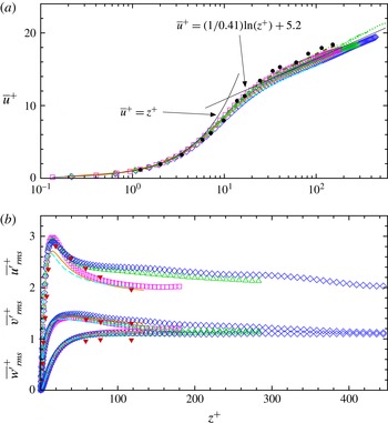
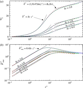
). Additional validations for turbulent flows and scalar transport over a flat wall are given in appendix A.
3 Simulation configuration
For the simulations of turbulent flows over surface waves considered in this study, the flow is driven by a constant shear stress
 $\unicode[STIX]{x1D70F}_{x}$
applied on the top boundary of the simulation domain. The Reynolds number based on the friction velocity
 $u_{\ast }=\sqrt{\unicode[STIX]{x1D70F}_{x}/\unicode[STIX]{x1D70C}}$
and half of the mean domain height
 $\unicode[STIX]{x1D6FF}=\overline{H}/2$
is
 $Re_{\ast }=u_{\ast }\unicode[STIX]{x1D6FF}/\unicode[STIX]{x1D708}=445$
. To capture the effect of surface waves on the turbulence transport of scalars, a computational domain of
 $\left(L_{x},L_{y},\overline{H}\right)=\left(4\unicode[STIX]{x1D706},3\unicode[STIX]{x1D706},2\unicode[STIX]{x1D706}\right)$
is used, where the wavelength
 $\unicode[STIX]{x1D706}=\unicode[STIX]{x1D6FF}$
. This domain size has been found to be sufficiently large based on the test of two-point spatial correlation (Yang & Shen Reference Yang and Shen2009). The domain is transformed into the computational space
 $(\unicode[STIX]{x1D709},\unicode[STIX]{x1D713},\unicode[STIX]{x1D701})$
based on (2.12), and then discretized using
 $192^{3}$
grid points. In particular, the grid points are evenly spaced in the
 $\unicode[STIX]{x1D709}$
- and
 $\unicode[STIX]{x1D713}$
-directions, providing grid resolutions of
 $\unicode[STIX]{x0394}\unicode[STIX]{x1D709}^{+}=9.27$
and
 $\unicode[STIX]{x0394}\unicode[STIX]{x1D713}^{+}=6.95$
, respectively (here the subscript ‘
 $+$
’ denotes the length in wall unit, i.e. normalized by
 $\unicode[STIX]{x1D708}/u_{\ast }$
). In the vertical direction, the grid points are clustered near the bottom and top boundaries with
 $\unicode[STIX]{x0394}\unicode[STIX]{x1D701}^{+}=0.4$
, and become coarsely spaced towards the centre of the domain with
 $\unicode[STIX]{x0394}\unicode[STIX]{x1D701}^{+}=8.7$
.
Note that the Reynolds number considered in the current DNS study is lower than those used in DNS studies of turbulence over a flat surface (e.g. Hoyas & Jiménez Reference Hoyas and Jiménez2006; Lee & Moser Reference Lee and Moser2015) because of the additional complexity and computational cost caused by the boundary-fitted grid and coordinate transformation, but is higher than those used in many previous DNS studies of turbulence over progressive and stationary waves, e.g.
 $Re_{\ast }=171$
in De Angelis, Lombardi & Banerjee (Reference De Angelis, Lombardi and Banerjee1997),
 $Re_{\ast }=100\sim 164$
in Sullivan et al. (Reference Sullivan, McWilliams and Moeng2000) and Sullivan & McWilliams (Reference Sullivan and McWilliams2002),
 $Re_{\ast }=150$
in Kihara et al. (Reference Kihara, Hanazaki, Mizuya and Ueda2007),
 $Re_{\ast }=283$
in Yang & Shen (Reference Yang and Shen2010), and
 $Re_{\ast }=140\sim 325$
in Druzhinin, Troitskaya & Zilitinkevich (Reference Druzhinin, Troitskaya and Zilitinkevich2012) and Druzhinin et al. (Reference Druzhinin, Troitskayaa and Zilitinkevich2016). Although limited to relatively low Reynolds numbers, DNS has been found to be able to reproduce many key features of laboratory experiments and field observations (Sullivan & McWilliams Reference Sullivan and McWilliams2010). More importantly, DNS directly resolves the flow and scalar transport in the near-surface region, where molecular viscosity and diffusivity play an important role. Meirink & Makin (Reference Meirink and Makin2000) solved the Reynolds-averaged Navier–Stokes equations using a Dirichlet wave boundary condition and a second-order closure of Craft & Launder (Reference Craft and Launder1996) that is valid in the viscous sublayer, and reproduced the air flow over water waves measured by Stewart (Reference Stewart1970), suggesting the importance of capturing the viscous effect when modelling wind–wave interaction (Sullivan & McWilliams Reference Sullivan and McWilliams2010).
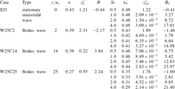
List of DNS cases for turbulent flow over stationary and Stokes waves with steepness
 $ak=0.25$
and Reynolds number
 $Re_{\ast }=445$
. In the table, the parameters without and with subscript ‘
 $\unicode[STIX]{x1D703}$
’ are for mean velocity and scalar profiles, respectively. In particular,
 $\unicode[STIX]{x1D705}$
is the von Kármán constant,
 $z_{0}^{+}$
is the effective wave surface roughness, and
 $B$
is the profile offset. Detailed discussions of the mean profiles are given in § 4.3.

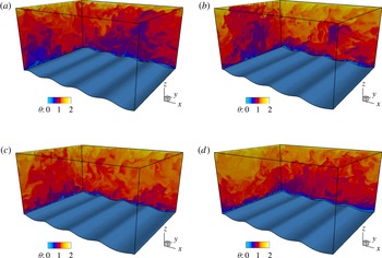
Three-dimensional illustration of instantaneous scalar field in turbulence over surface waves for various wave cases: (a) S25 (stationary wave); (b) W25C2 (slow wave); (c) W25C14 (intermediate wave); and (d) W25C25 (fast wave). For all cases, the contours of the instantaneous scalar concentration
 $\unicode[STIX]{x1D703}$
for
 $Sc=1.0$
are shown on the two representative vertical planes. The wave surface is shaded blue for illustrative purposes. In (b–d), the waves propagate in the
 $x$
-direction.

Because DNS usually uses relatively low Reynolds numbers to resolve all the essential turbulence motions at different scales, the velocity and length scales considered in the present and other similar studies in literature do not directly match the real scales in wind over water waves. Nevertheless, DNS has been proven to provide valuable insights for understanding the characteristics of wind turbulence over waves. Moreover, previous studies have shown that the wave age, defined as the ratio of the wave phase speed
 $c$
to a characteristic wind velocity, is a key parameter for the quantitative description of wind–wave interaction (see the reviews by Belcher & Hunt Reference Belcher and Hunt1998; Sullivan & McWilliams Reference Sullivan and McWilliams2010). Typical choices of the characteristic wind velocity include: (1) the wind friction velocity,
 $u_{\ast }$
(e.g. Belcher & Hunt Reference Belcher and Hunt1998; Sullivan et al.
Reference Sullivan, McWilliams and Moeng2000; Kihara et al.
Reference Kihara, Hanazaki, Mizuya and Ueda2007; Yang & Shen Reference Yang and Shen2009, Reference Yang and Shen2010); (2) the mean wind velocity at a height proportional to the wavelength
 $\unicode[STIX]{x1D706}$
, e.g.
 $U_{\unicode[STIX]{x1D706}}$
at
 $z=\unicode[STIX]{x1D706}$
or
 $U_{\unicode[STIX]{x1D706}/2}$
at
 $z=\unicode[STIX]{x1D706}/2$
(e.g. Sullivan et al.
Reference Sullivan, McWilliams and Moeng2000; Donelan et al.
Reference Donelan, Babanin, Young and Banner2006); and (3) the mean wind velocity at a fixed height above the mean wave surface regardless of the wavelength, e.g.
 $U_{10}$
at the
 $10\,\text{m}$
height (see, e.g., Hristov, Miller & Friehe Reference Hristov, Miller and Friehe2003; Donelan et al.
Reference Donelan, Babanin, Young and Banner2006, among others). In this study, because the carrier flow is driven by a prescribed stress
 $\unicode[STIX]{x1D70F}_{x}$
that gives a constant friction velocity
 $u_{\ast }$
, it is most convenient to define the wave age as
 $c/u_{\ast }$
.
To study the effect of surface wave motion on the scalar transport, three different wave ages are considered,
 $c/u_{\ast }=2$
,
 $14$
and
 $25$
, corresponding to the young, intermediate and mature stages of wind-generated waves, respectively (Belcher & Hunt Reference Belcher and Hunt1998). Moreover, if
 $c=0$
, the bottom boundary becomes a stationary wavy wall without orbital motion, which has often been used as a reference case for comparison in many prior numerical studies of flows over surface waves. All of the four wave cases have a wave steepness of
 $ak=0.25$
. The wave cases considered in the present study are summarized in table 1. For each wave case, four Schmidt numbers,
 $Sc=0.5$
,
 $1.0$
,
 $2.0$
and
 $4.0$
, are considered in the DNS for the scalar transport. Figure 2 shows some sample DNS results for the instantaneous scalar concentration field in turbulence over the four different types of waves with
 $Sc=1.0$
. Apparent differences in the instantaneous scalar field can be observed among the stationary (S25), slow (W25C2) and intermediate (W25C14) wave cases, while the difference between the intermediate and fast (W25C25) wave cases is less obvious. To quantitatively study the effect of surface waves on scalar transport, in the next section various statistical analyses are performed for the scalar field. For data sampling, in all the cases the simulations were carried out for approximately
 $34\,000$
viscous time units (i.e.
 $tu_{\ast }^{2}/\unicode[STIX]{x1D708}$
). Three-dimensional snapshots of instantaneous velocity and scalar fields were outputted for every
 $20$
viscous time units starting from approximately
 $26\,000$
viscous time units, with totally
 $400$
instantaneous snapshots sampled for the statistical analyses.
4 Results
4.1 Phase-averaged scalar field
To quantify the effect of surface waves on the turbulent flow and scalar fields, a triple decomposition is applied to analyze the instantaneous quantities. Specifically, an instantaneous quantity
 $f(x,y,z,t)$
obtained from the DNS can be decomposed as (e.g. Sullivan et al.
Reference Sullivan, McWilliams and Moeng2000; Kihara et al.
Reference Kihara, Hanazaki, Mizuya and Ueda2007; Yang & Shen Reference Yang and Shen2010)
 $$\begin{eqnarray}f(x,y,z,t)=\langle f\rangle (x,z)+f^{\prime }(x,y,z,t)=\overline{f}(\unicode[STIX]{x1D701})+\widetilde{f}(x,z)+f^{\prime }(x,y,z,t),\end{eqnarray}$$
where
 $\langle f\rangle$
denotes the phase average,
 $\overline{f}$
denotes the time and
 $\unicode[STIX]{x1D701}$
-plane average over all
 $(\unicode[STIX]{x1D709},\unicode[STIX]{x1D713},\unicode[STIX]{x1D70F})$
in the computational space (hereinafter simply referred to as the time and plane average),
 $\widetilde{f}$
denotes the wave-induced variation of
 $f$
, and
 $f^{\prime }$
denotes the instantaneous fluctuation. In particular, the phase average
 $\langle f\rangle$
is calculated by shifting the instantaneous quantity
 $f$
to the same phase with respect to the surface wave, then averaging in time and along the spanwise direction, and lastly further averaging among the four streamwise waves (Yang & Shen Reference Yang and Shen2010). The wave-induced variation is then obtained by subtracting from the phase average the time and plane average at the corresponding
 $\unicode[STIX]{x1D701}$
level in the computational space, i.e.
 $\widetilde{f}(x,z)=\langle f\rangle (x,z)-\overline{f}(\unicode[STIX]{x1D701})$
. As a result of the averaging among the four different waves, only one wavelength is necessary when presenting
 $\langle f\rangle$
and
 $\widetilde{f}$
. Moreover, when presenting the vertical profile of the time and plane average
 $\overline{f}$
, the
 $\unicode[STIX]{x1D701}$
coordinate is converted to the physical coordinate above the wave surface as
 $\overline{z}=\overline{H}\unicode[STIX]{x1D701}$
(for a flat-surface case,
 $\overline{z}=z$
). Hereinafter, for simplification
 $\overline{f}$
is also referred to as the mean of
 $f$
.
Note that to calculate the mean, one could also choose to first interpolate the physical quantities obtained from the boundary-fitted DNS to a regular Cartesian grid and then average on planes of constant
 $z$
. However, by doing so the flow region below the height of the wave crest would be excluded (e.g. Rutgersson & Sullivan Reference Rutgersson and Sullivan2005). As shown in the following subsections, because the current DNS uses boundary-fitted grid with the
 $\unicode[STIX]{x1D701}$
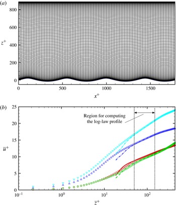
-plane nearly parallel to the wave surface near the lower boundary (see figure 29
a in appendix B), calculating
 $\overline{f}$
by averaging on planes of constant
 $\unicode[STIX]{x1D701}$
allows us to capture the linear profiles of mean velocity and scalar in the thin viscous sublayer very close to the wave surface. Meanwhile, in the log-law region the difference of the mean profiles obtained by averaging on
 $z$
planes and
 $\unicode[STIX]{x1D701}$
planes is found to be small because the
 $\unicode[STIX]{x1D701}$
plane becomes flatter as
 $\unicode[STIX]{x1D701}$
increases (see more information in appendix B). Moreover, defining and calculating
 $\overline{f}$
based on
 $\unicode[STIX]{x1D701}$
allows us to have meaningful values for the wave-correlated variation
 $\widetilde{f}$
in the entire phase-averaged domain, including the region above the trough but below the elevation of the crest. Similar triple decomposition approaches as (4.1) have been used in previous studies of turbulent flows over waves (e.g. Sullivan et al.
Reference Sullivan, McWilliams and Moeng2000; Sullivan & McWilliams Reference Sullivan and McWilliams2002; Kihara et al.
Reference Kihara, Hanazaki, Mizuya and Ueda2007; Hara & Sullivan Reference Hara and Sullivan2015).
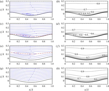
Phase-averaged (a,c,e,g) streamlines and (b,d,f,h) scalar concentration
 $\langle \unicode[STIX]{x1D703}\rangle$
(for
 $Sc=1.0$
) for various wave cases: (a,b) S25; (c,d) W25C2; (e,f) W25C14; and (g,h) W25C25. The streamlines are based on
 $(\langle u\rangle -c,\langle w\rangle )$
, i.e. in the reference frame moving with the wave phase speed
 $c$
. The red dash-dot line indicates the location of the critical layer where
 $\langle u\rangle -c=0$
(it is located higher than
 $z/\unicode[STIX]{x1D706}=0.3$
in case W25C25 and thus is not shown in (g)). The contour interval for
 $\langle \unicode[STIX]{x1D703}\rangle$
is
 $0.1$
.

Comparison of phase-averaged scalar concentration
 $\langle \unicode[STIX]{x1D703}\rangle$
with
 $Sc=0.7$
over a stationary wavy wall with steepness
 $ak=0.314$
. Profiles of
 $\langle \unicode[STIX]{x1D703}\rangle$
at
 $x/\unicode[STIX]{x1D706}=0.1$
,
 $0.3$
,
 $0.5$
, and
 $0.7$
are plotted:
 $\circ$
, DNS of channel flow by Rossi (Reference Rossi2010);
 $-\!\!\!-\!\!\!-$
, current DNS with
 $Re_{\ast }=283$
. The reference value
 $\unicode[STIX]{x1D703}_{ref}$
for the normalization is based on the mean scalar concentration at
 $z=0.3\unicode[STIX]{x1D706}$
.

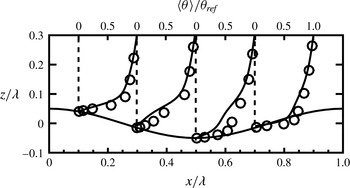
Figure 3 shows the phase-averaged streamlines and scalar concentration
 $\langle \unicode[STIX]{x1D703}\rangle$
for various wave cases. The streamlines are plotted based on the velocity vector
 $(\langle u\rangle -c,\langle w\rangle )$
, representing the mean flow pattern in the wave-following reference frame. In case S25 (figure 3
a), due to the large amplitude of the stationary wavy surface, the phase-averaged flow separates on the leeward face of the crest and reattaches on the windward face of the succeeding crest. The streamlines in the separation zone exhibit a closed-circle pattern, which does not extend vertically beyond the elevation of the wave crest. Above the separation zone, the streamlines are nearly horizontal, with a slightly concave curvature above the reattachment region. The distribution of the phase-averaged scalar concentration
 $\langle \unicode[STIX]{x1D703}\rangle$
exhibits correlation with the streamline patterns (figure 3
b). Near the wavy surface, the low-
 $\langle \unicode[STIX]{x1D703}\rangle$
region is lifted up in the separation zone between the crest and the succeeding trough (i.e. roughly between
 $x/\unicode[STIX]{x1D706}=0.1$
and
 $0.5$
) due to the mean upward flow motion associated with the separation, resulting in a reduced vertical gradient for
 $\langle \unicode[STIX]{x1D703}\rangle$
; near the reattachment zone (i.e. around
 $x/\unicode[STIX]{x1D706}=0.7$
), the mean flow sweeps towards the windward face of the succeeding crest, resulting in a strong near-surface shear layer (from
 $x/\unicode[STIX]{x1D706}=0.6$
to
 $1.0$
) with a high vertical gradient for both
 $\langle u\rangle$
and
 $\langle \unicode[STIX]{x1D703}\rangle$
. These wave-phase-dependent modulations of the near-surface distribution of
 $\langle \unicode[STIX]{x1D703}\rangle$
are revisited when the Sherwood number
 $Sh$
is discussed in the next section (§ 4.2). Above the elevation of the crest, the contour lines of
 $\langle \unicode[STIX]{x1D703}\rangle$
become nearly horizontal, consistent with the horizontal streamlines at these high elevations. Similar near-surface modulation of
 $\langle \unicode[STIX]{x1D703}\rangle$
has also been reported in the DNS study by Rossi (Reference Rossi2010) for transport of a scalar with
 $Sc=0.7$
in a turbulent channel flow over a stationary wavy surface with steepness
 $ak=0.314$
. Figure 4 shows a corresponding case obtained from our DNS (with
 $ak=0.314$
and
 $Re_{\ast }=283$
), which yields reasonably good agreement with the DNS results from Rossi (Reference Rossi2010).
In case W25C2 (figure 3
c,d), the wave surface has non-zero orbital velocities
 $(u_{s},w_{s})$
that induce additional distortion to the flow field above it (in addition to the boundary curvature effect as in case S25). In the reference frame that moves with the wave at its phase speed
 $c$
, near the surface the mean streamwise velocity
 $\langle u\rangle -c$
is in the
 $-x$
-direction. As
 $\langle u\rangle$
increases with height,
 $\langle u\rangle -c$
becomes zero at the height indicated by the dash-dot line in figure 3(c), and becomes positive further above. The layer where
 $\langle u\rangle -c=0$
, known as the ‘critical layer’, was found to play a crucial role in the momentum transfer between the turbulence and the surface waves (e.g. Miles Reference Miles1957; Lighthill Reference Lighthill1962; Sullivan et al.
Reference Sullivan, McWilliams and Moeng2000; Hristov et al.
Reference Hristov, Miller and Friehe2003). Around the critical layer, the streamlines form a closed-circle pattern, named as the ‘cat’s eye’ by Lighthill (Reference Lighthill1962). For case W25C2, the cat’s-eye streamlines are located right above the wave trough. Note that the cat’s eyes pattern in figure 3(c) does not imply the occurrence of mean flow separation above the wave trough (see Banner & Melville Reference Banner and Melville1976; Gent & Taylor Reference Gent and Taylor1977). Unlike in the flow over a stationary wave, in which a negative surface stress (i.e. reversed near-surface flow) would indicate a flow separation, in flows over progressive waves the near-surface flow is in the reversed direction in the wave-following reference frame everywhere above the wave surface. Yang & Shen (Reference Yang and Shen2010) used the local relative velocity (with respect to the local surface orbital velocity) and found occasional instantaneous flow separations occur on the leeward face of slow progressive waves, while the mean flow was found to remain unseparated. Similarly, in case W25C2 of the current DNS the mean flow is found to be unseparated. Compared with the mean flow separation bubble in case S25, in case W25C2 the cat’s-eye streamline pattern extends further upwards and upstream, As a result, the low-
 $\langle \unicode[STIX]{x1D703}\rangle$
region above the wave trough is lifted further upwards, and this effect also extends further upstream when compared with case S25.
For cases W25C14 (figure 3
e,f) and W25C25 (figure 3
g,h), the wave phase speed
 $c$
is large and the critical layer is located far from the wave surface. Below the critical layer, the streamlines are nearly parallel to the wave surface with the mean streamwise velocity
 $\langle u\rangle -c$
in the
 $-x$
-direction. Associated with this smooth streamline pattern, the contour lines for
 $\langle \unicode[STIX]{x1D703}\rangle$
are also nearly parallel to the wave surface. In cases W25C14 and W25C25 the scalar concentration
 $\langle \unicode[STIX]{x1D703}\rangle$
near the wave surface is in general higher than that in cases S25 and W25C2, as indicated by the lower elevations of the
 $\langle \unicode[STIX]{x1D703}\rangle =0.6$
and
 $0.8$
contour lines, respectively, in figures 3(f) and 3(h) compared with those in figures 3(b) and 3(d).
Distribution of wave-induced variation of scalar concentration,
 $\widetilde{\unicode[STIX]{x1D703}}$
, for various wave cases: (a,e) S25; (b,f) W25C2; (c,g) W25C14; and (d,h) W25C25. (a–d) Show the contours of
 $\widetilde{\unicode[STIX]{x1D703}}$
for
 $Sc=1.0$
. The contour intervals are (a,e)
 $0.04$
, (b,f)
 $0.04$
, (c,g)
 $0.01$
and (d,h)
 $0.01$
. Dashed contour lines indicate negative values. (e–h) Show the vertical profiles of
 $\overline{|\widetilde{\unicode[STIX]{x1D703}}|}$
(i.e. the average of
 $|\widetilde{\unicode[STIX]{x1D703}}|$
over all
 $\unicode[STIX]{x1D709}$
) for various values of
 $Sc$
: ——,
 $Sc=0.5$
; – – –,
 $Sc=1.0$
; — ⋅ —,
 $Sc=2.0$
; and — ⋅ ⋅ —,
 $Sc=4.0$
.

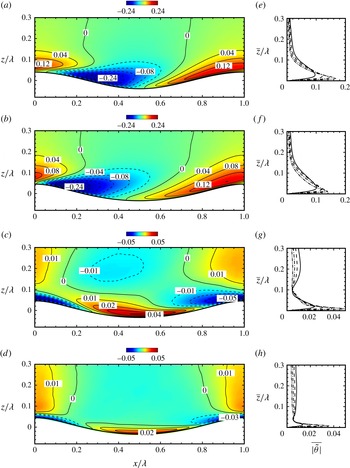
The effect of surface waves on the scalar field can be directly visualized from the distribution of the wave-induced variation of the scalar concentration,
 $\widetilde{\unicode[STIX]{x1D703}}$
, in which the time and plane average
 $\overline{\unicode[STIX]{x1D703}}$
has been removed. Figure 5 shows the two-dimensional contours of
 $\widetilde{\unicode[STIX]{x1D703}}$
and the vertical profile of the
 $\unicode[STIX]{x1D709}$
-average of its magnitude,
 $\overline{|\widetilde{\unicode[STIX]{x1D703}}|}$
. For cases S25 (figure 5
a) and W25C2 (figure 5
b), the distribution of
 $\widetilde{\unicode[STIX]{x1D703}}$
is asymmetric about the wave crest, with negative values above the leeward face and trough, and positive values above the windward face and crest. For cases W25C14 (figure 5
c) and W25C25 (figure 5
d), the distribution of
 $\widetilde{\unicode[STIX]{x1D703}}$
becomes nearly symmetric with respect to the wave trough, with positive values above the trough and negative values above the crest. For all the four wave cases, the averaged magnitude
 $\overline{|\widetilde{\unicode[STIX]{x1D703}}|}$
has its maximum near the wave surface (at
 $\unicode[STIX]{x1D701}/\unicode[STIX]{x1D706}\lesssim 0.04$
), and reduces to a small value at higher height. The peak values of
 $\overline{|\widetilde{\unicode[STIX]{x1D703}}|}$
for cases S25 and W25C2 are significantly higher than those for cases W25C14 and W25C25. Figure 5 also shows the effect of
 $Sc$
on
 $\overline{|\widetilde{\unicode[STIX]{x1D703}}|}$
. For all of the cases, the increase of
 $Sc$
causes an increase of the peak value and a reduction in the height of the peak.
4.2 Sherwood number
The wave-induced variation of the near-surface scalar field causes considerable wave-correlated variation in the Sherwood number. The Sherwood number is usually used to measure the relative importance of convection and molecular diffusion in convective mass transfer processes (corresponding to the Nusselt number in heat transfer). The local Sherwood number along the wave surface based on the phase-averaged scalar field can be calculated as
 $$\begin{eqnarray}\displaystyle Sh\equiv \frac{h\overline{H}/2}{D}=\frac{\displaystyle \left.\frac{\unicode[STIX]{x2202}\langle \unicode[STIX]{x1D703}\rangle }{\unicode[STIX]{x2202}z}\right|_{z=\unicode[STIX]{x1D702}}\overline{H}}{2(\overline{\unicode[STIX]{x1D703}}_{1/2}-\unicode[STIX]{x1D703}_{0})}, & & \displaystyle\end{eqnarray}$$
where
 $h$
is the convective mass transfer coefficient,
 $D$
is the molecular diffusivity as in (2.3),
 $\overline{\unicode[STIX]{x1D703}}_{1/2}$
is the averaged
 $\unicode[STIX]{x1D703}$
at the centre height of the domain (
 $\overline{z}=\overline{H}/2$
), and
 $\unicode[STIX]{x1D703}_{0}=0$
is the imposed bottom surface value of
 $\unicode[STIX]{x1D703}$
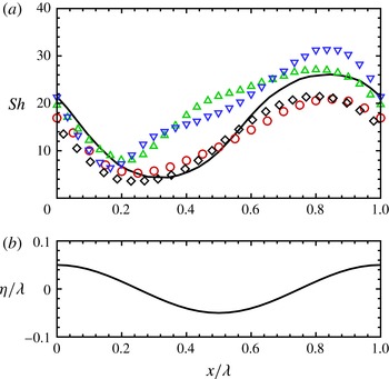
as the boundary condition. Figure 6 shows the wave-correlated variation of
 $Sh$
for the steep stationary wave case (i.e. the case with
 $ak=0.314$
and
 $Re_{\ast }=283$
as shown in figure 4), in which the current DNS result is compared with the results from several previous numerical studies (Park et al.
Reference Park, Choi and Suzuki2004; Dellil et al.
Reference Dellil, Azzi and Jubran2004; Choi & Suzuki Reference Choi and Suzuki2005). For the steep stationary wave case, the profile of
 $Sh$
has a nearly sinusoidal shape. On the stationary wavy surface, the value of
 $Sh$
is small above the leeward face and large above the windward face, as a result of the smaller and larger vertical gradients of
 $\langle \unicode[STIX]{x1D703}\rangle$
on the leeward and windward faces, respectively, as shown in figures 3(a) and 4.
(a) Profiles of phase-averaged local Sherwood number
 $Sh$
over the stationary wavy wall: ○, RANS result of Park et al. (Reference Park, Choi and Suzuki2004) for
 $(ak,Sc)=(0.1\unicode[STIX]{x03C0},0.7)$
; ▫, RANS result of Dellil et al. (Reference Dellil, Azzi and Jubran2004) for
 $(ak,Sc)=(0.08\unicode[STIX]{x03C0},0.9)$
; ▵, RANS result of Dellil et al. (Reference Dellil, Azzi and Jubran2004) for
 $(ak,Sc)=(0.12\unicode[STIX]{x03C0},0.9)$
; ▿, LES result of Choi & Suzuki (Reference Choi and Suzuki2005) for
 $(ak,Sc)=(0.1\unicode[STIX]{x03C0},0.7)$
; and ——, current DNS result for
 $(ak,Sc)=(0.1\unicode[STIX]{x03C0},0.7)$
and
 $Re_{\ast }=283$
(see figure 4). The corresponding wave surface phase is indicated by the wave elevation
 $\unicode[STIX]{x1D702}$
of
 $ak=0.1\unicode[STIX]{x03C0}$
in panel (b).

(a) Profiles of phase-averaged local Sherwood number
 $Sh$
for
 $Sc=1.0$
and for various wave cases: ○, S25 (
 $c/u_{\ast }=0$
); ▫, W25C2 (
 $c/u_{\ast }=2$
); ▵, W25C14 (
 $c/u_{\ast }=14$
); and ▿, W25C25 (
 $c/u_{\ast }=25$
). The corresponding wave surface phase is indicated by the wave elevation
 $\unicode[STIX]{x1D702}$
in panel (b).

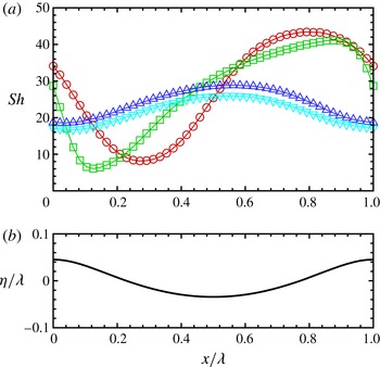
Figure 7 shows the effect of wave motion on
 $Sh$
. The plotted curves are for
 $Sc=1.0$
. When the wave is slow (case W25C2), similar to the stationary wave condition,
 $Sh$
is also small above the leeward face and large above the windward face. However, the shape of the
 $Sh$
curve apparently differs from the sinusoidal shape, with its minimum point closer to the wave crest (near
 $x/\unicode[STIX]{x1D706}=0.12$
). For cases with intermediate (case W25C14) and fast (W25C25) waves, the distribution of
 $Sh$
become symmetric with respect to the wave form, with the maxima above the wave trough and the minima above the crest, corresponding to the regions of positive and negative
 $\widetilde{\unicode[STIX]{x1D703}}$
in figure 5, respectively.
Dependence of mean Sherwood number
 $\overline{Sh}$
on
 $Sc$
for various wave cases: ○, S25 (
 $c/u_{\ast }=0$
); ▫, W25C2 (
 $c/u_{\ast }=2$
); ▵, W25C14 (
 $c/u_{\ast }=14$
); and ▿, W25C25 (
 $c/u_{\ast }=25$
). The lines are the curve fittings: – – –,
 $\overline{Sh}=27.09Sc^{0.579}$
for S25; — ⋅ —,
 $\overline{Sh}=26.54Sc^{0.609}$
for W25C2;
 $\cdots \,$
,
 $\overline{Sh}=23.68Sc^{0.514}$
for W25C14; and — ⋅ ⋅ —,
 $\overline{Sh}=21.13Sc^{0.518}$
for W25C25. The two solid lines show the averaged slope of the four surface wave conditions, i.e.
 $\overline{Sh}\propto Sc^{0.555}$
.

For a given wave condition, varying the
 $Sc$
value mainly causes changes in the magnitudes of the mean and variation of
 $Sh$
, while the shapes of the curves are similar to those of the corresponding curves shown in figure 7. Thus, these additional
 $Sh$
curves with different
 $Sc$
are not plotted here, and only the effect of
 $Sc$
on the averaged Sherwood number
 $\overline{Sh}$
(
 $=(1/\unicode[STIX]{x1D706})\int _{0}^{\unicode[STIX]{x1D706}}Sh(x)\text{d}x$
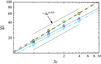
) is discussed. Figure 8 shows the dependence of
 $\overline{Sh}$
on
 $Sc$
. Previous studies on scalar transport in wall-bounded or free-surface-bounded turbulent flows have shown that the scaling of
 $\overline{Sh}$
with
 $Sc$
follows a power law (e.g. Shaw & Hanratty Reference Shaw and Hanratty1977; Jähne & Haußecker Reference Jähne and Haußecker1998; Na, Papavassiliou & Hanratty Reference Na, Papavassiliou and Hanratty1999; Hasegawa & Kasagi Reference Hasegawa and Kasagi2008), i.e.
 $$\begin{eqnarray}\overline{Sh}=\unicode[STIX]{x1D6FC}Sc^{\unicode[STIX]{x1D6FD}}.\end{eqnarray}$$
The current DNS results also exhibit this power-law trend for each wave condition as shown in figure 8. For the four different surface wave conditions considered in this study, the power-law coefficient
 $\unicode[STIX]{x1D6FD}$
varies slightly around an averaged value of
 $0.555$
, while
 $\unicode[STIX]{x1D6FC}$
varies between
 $21.13$
and
 $27.09$
. The pronounced variation of
 $\unicode[STIX]{x1D6FC}$
with the surface wave condition indicates the importance of wave motion on the magnitude of scalar transport. To further elucidate the effect of wave motion on scalar transport, the averaged Sherwood number
 $\overline{Sh}$
is plotted in figure 9 as a function of the wave age
 $c/u_{\ast }$
. When
 $Sc$
is fixed, in general
 $\overline{Sh}$
decreases as
 $c/u_{\ast }$
increases (figure 9
a). When normalized by
 $Sc^{0.555}$
(as suggested by the curve fitting in figure 8), the
 $\overline{Sh}$
curves for all the different Schmidt numbers collapse reasonably well.
Dependence of mean Sherwood number
 $\overline{Sh}$
on wave age
 $c/u_{\ast }$
for various Schmidt numbers:

 $Sc=0.5$
;

 $Sc=1.0$
;

 $Sc=2.0$
; and

 $Sc=4.0$
. In panel (b),
 $\overline{Sh}$
is rescaled by
 $Sc^{0.555}$
.

4.3 Profiles of time- and plane-averaged quantities
The phase-averaged statistics in § 4.1 have shown significant wave-induced variation in the scalar field, which is highly dependent on the wave phase. In many practical applications, the surface wave effect is usually not directly captured in a phase-resolved context. Instead, the averaged wave effect is parameterized as the effective wave roughness that appears in the one-dimensional profiles of the time- and plane-averaged velocity and scalar concentration, which can be obtained based on field and laboratory measurement data (e.g. Charnock Reference Charnock1955; Smith Reference Smith1988; Fairall et al.
Reference Fairall, Bradley, Rogers, Edson and Young1996; Johnson et al.
Reference Johnson, Høstrup, Vested and Larsen1998; Toba et al.
Reference Toba, Smith, Ebuchi, Jones and Toba2001). Although limited to low Reynolds number conditions, DNS has been shown to provide valuable insights for understanding the dependence of the effective wave roughness on the characteristics of the waves (Sullivan et al.
Reference Sullivan, McWilliams and Moeng2000). In this subsection, time and plane averaging is performed for the instantaneous snapshots of scalar and velocity fields obtained from the current DNS to help quantify the averaged wave effect. Note that the plane average is performed on the
 $\unicode[STIX]{x1D701}$
-plane in the computational space, as defined in § 4.1.
Profiles of mean streamwise velocity
 $\overline{u}^{+}$
for various wave cases: ○, S25 (
 $c/u_{\ast }=0$
); ▫, W25C2 (
 $c/u_{\ast }=2$
); ▵, W25C14 (
 $c/u_{\ast }=14$
); and ▿, W25C25 (
 $c/u_{\ast }=25$
). The semi-logarithmic plot in panel (a) highlights the log-law region, with the thin solid lines indicating the logarithmic law
 $\overline{u}^{+}=(1/\unicode[STIX]{x1D705})\ln (\overline{z}^{+}/z_{0}^{+})$
and the corresponding values of
 $\unicode[STIX]{x1D705}$
and
 $z_{0}^{+}$
for each simulation case given in table 1. The logarithmic plot in panel (b) highlights the near-wall viscous layer, with the thin solid lines indicating the linear law
 $\overline{u}^{+}=\overline{z}^{+}$
. In the figure, the DNS result of flat-boundary channel flow from Kim, Moin & Moser (Reference Kim, Moin and Moser1987) is indicated by the thick line, and the experimental data from Eckelmann (Reference Eckelmann1974) (corrected by Kim et al.
Reference Kim, Moin and Moser1987) are indicated by the filled circles.

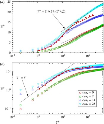
Figure 10 shows the profiles of the mean streamwise velocity
 $\overline{u}$
(for the definition, see (4.1) and the associated discussion). The slow wave case (W25C2,
 $c/u_{\ast }=2$
) shows a mean velocity profile close to that of the stationary wave case (S25). As
 $c/u_{\ast }$
increases, the profile of
 $\overline{u}^{+}$
shifts monotonically towards higher values, which is expected since the wave form drag decreases as
 $c/u_{\ast }$
increases (Belcher & Hunt Reference Belcher and Hunt1998). For the current DNS, the normalized pressure-induced form drag
 $F_{p}$
and surface viscous drag
 $F_{\unicode[STIX]{x1D708}}$
per unit projected horizontal area can be calculated based on the phase-averaged pressure and velocity as
 $$\begin{eqnarray}\displaystyle & \displaystyle F_{p}=\frac{1}{u_{\ast }^{2}\unicode[STIX]{x1D706}}\int _{0}^{\unicode[STIX]{x1D706}}\frac{\langle p\rangle }{\unicode[STIX]{x1D70C}}\frac{\unicode[STIX]{x2202}\unicode[STIX]{x1D702}}{\unicode[STIX]{x2202}x}\,\text{d}x, & \displaystyle\end{eqnarray}$$
 $$\begin{eqnarray}\displaystyle & \displaystyle F_{\unicode[STIX]{x1D708}}=\frac{1}{u_{\ast }^{2}\unicode[STIX]{x1D706}}\int _{0}^{\unicode[STIX]{x1D706}}\unicode[STIX]{x1D708}\left[\left(\frac{\unicode[STIX]{x2202}\langle u\rangle }{\unicode[STIX]{x2202}z}+\frac{\unicode[STIX]{x2202}\langle w\rangle }{\unicode[STIX]{x2202}x}\right)-2\frac{\unicode[STIX]{x2202}\langle u\rangle }{\unicode[STIX]{x2202}x}\frac{\unicode[STIX]{x2202}\unicode[STIX]{x1D702}}{\unicode[STIX]{x2202}x}\right]\,\text{d}x, & \displaystyle\end{eqnarray}$$
and the total surface drag per unit area equals to their sum,
 $F_{total}=F_{p}+F_{\unicode[STIX]{x1D708}}$
. As shown in figure 11, in cases S25 and W25C2, the form drag makes a significant contribution to the total surface drag. In case W25C14, the form drag is very small and the total surface drag is mostly due to the viscous effect, indicating that the mean flow and the surface wave are nearly in equilibrium. In case W25C25, the wave phase speed is fast and the surface wave pushes the mean flow forwards, resulting in negative form drag (i.e. a thrust). A similar dependence of the surface drag on the wave age has been reported in various previous studies (e.g. Li et al.
Reference Li, Xu and Taylor2000; Sullivan et al.
Reference Sullivan, McWilliams and Moeng2000; Kihara et al.
Reference Kihara, Hanazaki, Mizuya and Ueda2007; Yang & Shen Reference Yang and Shen2010).
Budget of surface drag as a function of wave age:

 $f_{total}$
;

 $f_{p}$
; and

 $f_{\unicode[STIX]{x1D708}}$
.

For all the four wave conditions considered in this study, the mean velocity profiles exhibit a distinct logarithmic region, as indicated by the thin solid lines in the semi-logarithmic plot in figure 10(a). These lines are determined by fitting the mean velocity profiles in the range of
 $\overline{z}^{+}\in [50,150]$
(see appendix B) with the logarithmic profile
 $$\begin{eqnarray}\overline{u}^{+}=\frac{1}{\unicode[STIX]{x1D705}}\ln \left(\overline{z}^{+}/z_{0}^{+}\right)=\frac{1}{\unicode[STIX]{x1D705}}\ln (\overline{z}^{+})+B,\end{eqnarray}$$
where the superscript ‘
 $+$
’ denotes the quantities normalized by the wall units (i.e. velocity is normalized by
 $u_{\ast }$
and length is normalized by
 $\unicode[STIX]{x1D708}/u_{\ast }$
),
 $\unicode[STIX]{x1D705}$
is the von Kármán constant,
 $z_{0}^{+}$
is the effective wave surface roughness, and
 $B$
is the profile offset. For each case, the corresponding log-law profile parameters
 $\unicode[STIX]{x1D705}$
,
 $z_{0}^{+}$
and
 $B$
are listed in table 1. Similar to the DNS results reported in Sullivan et al. (Reference Sullivan, McWilliams and Moeng2000), the evaluated
 $z_{0}^{+}$
values in most of the DNS cases considered in this study fall in the transitional regime (
 $0.1<z_{0}^{+}<2.2$
) in terms of the sea-surface roughness, which was categorized to be a common sea state by Kitaigorodskii & Donelan (Reference Kitaigorodskii, Donelan, Brutsaert and Jirka1984). The slow wave case W25C2 exhibits a roughness of
 $z_{0}^{+}=2.31$
that is slightly higher than the upper bound of the transitional regime. For cases S25, W25C2 and W25C14, the values for
 $\unicode[STIX]{x1D705}$
are close to the standard value of
 $\unicode[STIX]{x1D705}=0.41$
for the flat-wall case. The fast wave case W25C25 exhibits a smaller value of
 $\unicode[STIX]{x1D705}=0.27$
, which is likely due to the strong surface motion of the fast propagating surface waves when
 $c/u_{\ast }=25$
. Similarly, Sullivan et al. (Reference Sullivan, McWilliams and Moeng2000) reported a
 $10\,\%$
reduction of
 $\unicode[STIX]{x1D705}$
in DNS of turbulence over progressive waves with
 $ak=0.1$
(i.e. the waves are less steep than the ones studied here). Note that due to this smaller
 $\unicode[STIX]{x1D705}$
in case W25C25, its evaluated
 $z_{0}^{+}$
is larger than that in case W25C14. Therefore, the larger
 $z_{0}^{+}$
in case W25C25 does not imply that the turbulence sees the fast wave ‘rougher’ than the intermediate wave. It should be pointed out that caution should be taken when interpreting the mean velocity profile for the present fast wave case due to the limited Reynolds number used in this study. Under real oceanic conditions, the fast wave case usually corresponds to the wind over storm-generated ocean swells, for which the Reynolds number is much higher than what a DNS can afford. The current DNS of
 $c/u_{\ast }=25$
are more relevant to the condition of light wind over fast mechanically generated waves in laboratory-scale wind–wave tanks (e.g. Buckley & Veron Reference Buckley and Veron2016). Further study is required in the future in order to understand the effect of surface waves on the von Kármán constant and the wave surface roughness.
The near-surface behaviour of the mean velocity profile is shown by the logarithmic plot in figure 10(b). The mean velocity profiles exhibit a nearly linear behaviour in the viscous sublayer (i.e.
 $\overline{z}^{+}<5$
), with some non-negligible difference from the linear law of the flat-wall turbulence. In particular, the viscous sublayer profiles of the intermediate (W25C14) and fast (W25C25) wave cases are close to the linear profile of the flat-wall case (e.g. Kim et al.
Reference Kim, Moin and Moser1987; Lee & Moser Reference Lee and Moser2015), i.e.
 $\overline{u}^{+}=\overline{z}^{+}$
, but with larger value towards the wave surface due to the positive mean streamwise surface orbital velocity of the nonlinear Stokes wave. On the other hand, the stationary (S25) and slow (W25C2) wave cases also show a linear profile in the viscous sublayer, but with a velocity deficit compared with the flat-wall linear law. The viscous sublayer profile of the stationary wave case (S25) is nearly parallel to that of the flat wall, while the one for the slow wave case (W25C2) is tilted slightly towards higher values when approaching the surface due to the positive mean surface orbital velocity of the Stokes waves.
Profiles of rescaled mean scalar concentration
 $\overline{\unicode[STIX]{x1D703}}\,^{+}/Sc$
. Panel (a) shows various wave cases with a fixed Schmidt number
 $Sc=1.0$
: ○, S25 (
 $c/u_{\ast }=0$
); ▫, W25C2 (
 $c/u_{\ast }=2$
); ▵, W25C14 (
 $c/u_{\ast }=14$
); and ▿, W25C25 (
 $c/u_{\ast }=25$
). Panel (b) shows case W25C14 (
 $c/u_{\ast }=14$
) with various Schmidt numbers: ●,
 $Sc=0.5$
; ▪,
 $Sc=1.0$
; ▴,
 $Sc=2.0$
; and ▾,
 $Sc=4.0$
. The profiles are shown on a logarithmic scale to highlight the near-wall region, with the solid line indicating the linear law
 $\overline{\unicode[STIX]{x1D703}}\,^{+}/Sc=\overline{z}^{+}$
. In panel (a), the DNS result from Kawamura et al. (Reference Kawamura, Ohsaka, Abe and Yamamoto1998) is also plotted (the thick line).

Profiles of mean scalar concentration
 $\overline{\unicode[STIX]{x1D703}}\,^{+}$
. The definitions of the symbols are the same as those in figure 12. The profiles are shown on a semi-logarithmic scale to highlight the log-law region, with the thin solid lines indicating the logarithmic law
 $\overline{\unicode[STIX]{x1D703}}\,^{+}=(1/\unicode[STIX]{x1D705}_{\unicode[STIX]{x1D703}})\ln (\overline{z}^{+}/z_{0,\unicode[STIX]{x1D703}}^{+})$
and the corresponding values of
 $\unicode[STIX]{x1D705}_{\unicode[STIX]{x1D703}}$
and
 $z_{0,\unicode[STIX]{x1D703}}^{+}$
for each simulation case given in table 1. In panel (a), the DNS result from Kawamura et al. (Reference Kawamura, Ohsaka, Abe and Yamamoto1998) is also plotted (the thick line).

A similar analysis can be done for the mean scalar concentration. By compiling a number of experimental datasets, Kader (Reference Kader1981) showed that the mean temperature and scalar concentration in fully developed turbulent boundary layers follow a linear profile in the viscous sublayer and a logarithmic profile in the log-law region. In the near-surface region, the Kader correlation suggests that
 $$\begin{eqnarray}\overline{\unicode[STIX]{x1D703}}\,^{+}/Sc=\overline{z}^{+}-Sc[c_{4}\overline{z}^{+4}+O(\overline{z}^{+5})],\end{eqnarray}$$
where
 $c_{4}\approx 1.5\times 10^{-4}$
as estimated based on the experimental data (Kader Reference Kader1981). Therefore, for the flat-wall case it is expected that
 $$\begin{eqnarray}\overline{\unicode[STIX]{x1D703}}\,^{+}\approx Sc\,\overline{z}\,^{+}\end{eqnarray}$$
to the leading order near the surface, with the deviation from this linear profile increasing towards larger
 $\overline{z}\,^{+}$
and with higher
 $Sc$
. Similar near-surface linear behaviour is found in the current DNS results over wave surfaces. Here
 $\overline{\unicode[STIX]{x1D703}}\,^{+}=\overline{\unicode[STIX]{x1D703}}/\unicode[STIX]{x1D703}_{\ast }$
, where
 $$\begin{eqnarray}\unicode[STIX]{x1D703}_{\ast }=\left.\frac{D}{u_{\ast }}\frac{\text{d}\overline{\unicode[STIX]{x1D703}}}{\text{d}\overline{z}}\right|_{\overline{z}=0}\end{eqnarray}$$
is a characteristic scalar scale (in the case of heat transfer,
 $\unicode[STIX]{x1D703}_{\ast }$
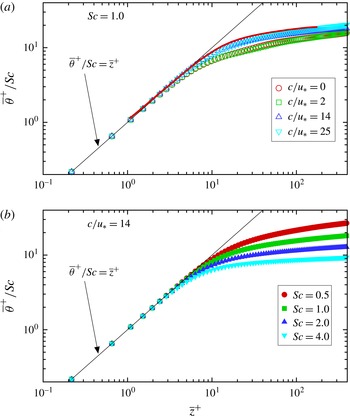
is also referred to as the friction temperature) (Kim & Moin Reference Kim, Moin, André, Cousteix, Durst, Launder, Schmidt and Whitelaw1989). Figure 12 shows the profiles of
 $\overline{\unicode[STIX]{x1D703}}\,^{+}/Sc$
(in a logarithmic plot) for some representative cases obtained by the current DNS. In particular, figure 12(a) shows the profiles for various wave cases with
 $Sc=1.0$
, and figure 12(b) shows the profiles for case W25C14 with various Schmidt numbers (other cases also follow consistent trends for the wave and
 $Sc$
dependences, and are thus not shown here due to space limitation). In the viscous sublayer (
 $\overline{z}^{+}<5$
), the profiles for different wave conditions and Schmidt numbers collapse well and agree with the linear law found in the flat-wall condition.
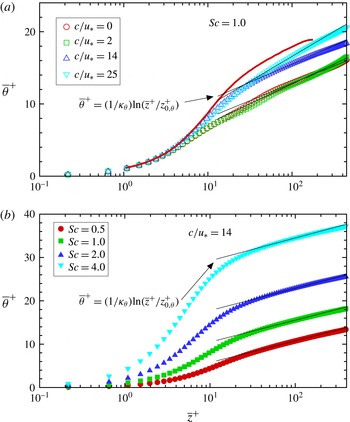
The logarithmic law behaviour of
 $\overline{\unicode[STIX]{x1D703}}\,^{+}$
can be visualized in a semi-logarithmic plot as shown in figure 13. Similar to the profile of
 $\overline{u}^{+}$
, for a fixed
 $Sc$
the
 $\overline{\unicode[STIX]{x1D703}}\,^{+}$
profile shifts towards higher values when
 $c/u_{\ast }$
increases, with the profile for
 $c/u_{\ast }=2$
close to that for the stationary wave case (figure 13
a). For each wave condition, the
 $\overline{\unicode[STIX]{x1D703}}\,^{+}$
profile shifts monotonically to higher values when
 $Sc$
increases (see for example the case W25C14 shown in figure 13
b). Similar to (4.6), the logarithmic law for scalar concentration can be written as (e.g. Kader Reference Kader1981)
 $$\begin{eqnarray}\displaystyle \overline{\unicode[STIX]{x1D703}}\,^{+}=\frac{1}{\unicode[STIX]{x1D705}_{\unicode[STIX]{x1D703}}}\ln (\overline{z}^{+}/z_{0,\unicode[STIX]{x1D703}}^{+})=\frac{1}{\unicode[STIX]{x1D705}_{\unicode[STIX]{x1D703}}}\ln \overline{z}^{+}+B_{\unicode[STIX]{x1D703}}, & & \displaystyle\end{eqnarray}$$
where
 $\unicode[STIX]{x1D705}_{\unicode[STIX]{x1D703}}$
is the von Kármán constant of scalar,
 $z_{0,\unicode[STIX]{x1D703}}^{+}$
is the effective wave surface roughness for scalar, and
 $B_{\unicode[STIX]{x1D703}}$
is the offset of the mean scalar profile. For each wave case, the corresponding parameters
 $\unicode[STIX]{x1D705}_{\unicode[STIX]{x1D703}}$
,
 $z_{0,\unicode[STIX]{x1D703}}^{+}$
, and
 $B_{\unicode[STIX]{x1D703}}$
can be obtained by fitting the DNS data in the log-law region (defined as
 $50<z^{+}<150$
in this study as explained in appendix B) with the logarithmic profile (4.10). The estimated values of these parameters are listed in table 1. For each wave case, the evaluated value of the scalar von Kármán constant
 $\unicode[STIX]{x1D705}_{\unicode[STIX]{x1D703}}$
exhibits a small variation when the Schmidt number is changed, while the profile offset
 $B_{\unicode[STIX]{x1D703}}$
(or the roughness
 $z_{0,\unicode[STIX]{x1D703}}^{+}$
) increases significantly as
 $Sc$
increases.
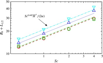
Dependence of
 $B_{\unicode[STIX]{x1D703}}$
on the Schmidt number for various wave cases: ○, S25 (
 $c/u_{\ast }=0$
); ▫, W25C2 (
 $c/u_{\ast }=2$
); ▵, W25C14 (
 $c/u_{\ast }=14$
); and ▿, W25C25 (
 $c/u_{\ast }=25$
). Equation (4.14) suggests that
 $B_{\unicode[STIX]{x1D703}}+L_{1/2}=Sc^{1-\unicode[STIX]{x1D6FD}}\overline{H}\,^{+}/(2\unicode[STIX]{x1D6FC})$
, as shown by the lines: – – –, S25; — ⋅ —, W25C2;
 $\cdots \,$
, W25C14; and — ⋅ ⋅ —, W25C25. For the current DNS,
 $\unicode[STIX]{x1D6FD}\approx 0.555$
when averaged among the four wave conditions, and the
 $\unicode[STIX]{x1D6FC}$
value for each wave condition can be found in the caption of figure 8.

The dependence of
 $B_{\unicode[STIX]{x1D703}}$
on
 $Sc$
can be further quantified. Recall that the averaged Sherwood number
 $\overline{Sh}$
follows a power-law dependence on
 $Sc$
, as shown in (4.3). Applying the surface average to (4.2) and combining it with (4.3) yields
 $$\begin{eqnarray}\unicode[STIX]{x1D6FC}Sc^{\unicode[STIX]{x1D6FD}}=\left.\frac{\text{d}\overline{\unicode[STIX]{x1D703}}\,^{+}}{\text{d}\overline{z}}\right|_{\overline{z}^{+}=0}\frac{\overline{H}\,^{+}}{2\overline{\unicode[STIX]{x1D703}}\,_{1/2}^{+}}.\end{eqnarray}$$
The near-surface linear profile (4.8) gives
 $$\begin{eqnarray}\left.\frac{\text{d}\overline{\unicode[STIX]{x1D703}}\,^{+}}{\text{d}\overline{z}}\right|_{\overline{z}^{+}=0}=Sc,\end{eqnarray}$$
and the logarithmic profile (4.10) gives
 $$\begin{eqnarray}\overline{\unicode[STIX]{x1D703}}\,_{1/2}^{+}=\frac{1}{\unicode[STIX]{x1D705}_{\unicode[STIX]{x1D703}}}\ln \left(\overline{H}\,^{+}/2\right)+B_{\unicode[STIX]{x1D703}}.\end{eqnarray}$$
Substituting (4.12) and (4.13) into (4.11) gives
 $$\begin{eqnarray}B_{\unicode[STIX]{x1D703}}=\frac{\overline{H}\,^{+}}{2\unicode[STIX]{x1D6FC}}Sc^{1-\unicode[STIX]{x1D6FD}}-L_{1/2},\end{eqnarray}$$
where
 $$\begin{eqnarray}L_{1/2}=\frac{1}{\unicode[STIX]{x1D705}_{\unicode[STIX]{x1D703}}}\ln \left(\overline{H}\,^{+}/2\right).\end{eqnarray}$$
As shown in table 1 and figure 9, for a given wave condition the parameters
 $\unicode[STIX]{x1D6FC}$
,
 $\unicode[STIX]{x1D6FD}$
and
 $\unicode[STIX]{x1D705}_{\unicode[STIX]{x1D703}}$
estimated based on the current DNS data are nearly constant. Therefore, equation (4.14) suggests that
 $B_{\unicode[STIX]{x1D703}}\sim Sc^{1-\unicode[STIX]{x1D6FD}}$
, where
 $\unicode[STIX]{x1D6FD}\approx 0.555$
as shown in § 4.2. Figure 14 shows the estimated
 $B_{\unicode[STIX]{x1D703}}+L_{1/2}$
as a function of the Schmidt number. With
 $\unicode[STIX]{x1D6FD}=0.555$
and
 $\unicode[STIX]{x1D6FC}$
given by the power-law fitting in figure 8, equation (4.14) is found to provide a reasonable parameterization for
 $B_{\unicode[STIX]{x1D703}}$
, which agrees well with the
 $B_{\unicode[STIX]{x1D703}}$
values obtained directly from the log-law profile fitting (the values are listed in table 1).
Profiles of (a)
 $\overline{\unicode[STIX]{x1D703}^{\prime }}\,\!_{rms}^{+}$
, (b)
 $\overline{\unicode[STIX]{x1D703}^{\prime }u^{\prime }}\,^{+}$
, and (c)
 $\overline{-\unicode[STIX]{x1D703}^{\prime }w^{\prime }}\,^{+}$
on a linear scale; and profiles of (d)
 $\unicode[STIX]{x1D703}_{rms}^{\prime +}/Sc$
, (e)
 $\overline{\unicode[STIX]{x1D703}^{\prime }u^{\prime }}\,^{+}/Sc$
, and (f)
 $\overline{-\unicode[STIX]{x1D703}^{\prime }w^{\prime }}\,^{+}/Sc$
on a logarithmic scale. The plotted DNS results are for
 $Sc=1.0$
with various wave cases: ○, S25 (
 $c/u_{\ast }=0$
); ▫, W25C2 (
 $c/u_{\ast }=2$
); ▵, W25C14 (
 $c/u_{\ast }=14$
); and ▿, W25C25 (
 $c/u_{\ast }=25$
). The solid lines in (d–f) indicate the expressions proposed by Kawamura et al. (Reference Kawamura, Ohsaka, Abe and Yamamoto1998).

4.4 Time- and plane-averaged statistics of scalar fluctuations
The presence of surface waves can induce a strong effect on the air turbulence. Statistics of velocity fluctuations above plane progressive waves of various wave ages and steepnesses have been studied in detail in previous studies (e.g. Sullivan et al. Reference Sullivan, McWilliams and Moeng2000; Kihara et al. Reference Kihara, Hanazaki, Mizuya and Ueda2007; Sullivan et al. Reference Sullivan, Edson, Hristov and McWilliams2008; Yang & Shen Reference Yang and Shen2010; Hara & Sullivan Reference Hara and Sullivan2015). On the other hand, the statistics of scalar fluctuations over waves have rarely been studied, with the exception of some studies for stationary wavy walls (e.g. Dellil et al. Reference Dellil, Azzi and Jubran2004; Park et al. Reference Park, Choi and Suzuki2004; Rossi Reference Rossi2010) and for stratified turbulence over water waves (e.g. Sullivan & McWilliams Reference Sullivan and McWilliams2002; Druzhinin et al. Reference Druzhinin, Troitskayaa and Zilitinkevich2016).
In this subsection, the time- and plane-averaged statistics of scalar fluctuations are studied based on the DNS data. Figure 15(a–c) shows the profiles of
 $\overline{\unicode[STIX]{x1D703}^{\prime }}\,\!_{rms}^{+}$
,
 $\overline{\unicode[STIX]{x1D703}^{\prime }u^{\prime }}\,^{+}$
, and
 $\overline{-\unicode[STIX]{x1D703}^{\prime }w^{\prime }}\,^{+}$
for various wave cases with
 $Sc=1.0$
. The profiles of
 $\overline{\unicode[STIX]{x1D703}^{\prime }}\,\!_{rms}^{+}$
(figure 15
a) and
 $\overline{\unicode[STIX]{x1D703}^{\prime }u^{\prime }}\,^{+}$
(figure 15
b) have a similar trend. As
 $\overline{z}^{+}$
increases from
 $0$
, the value first increases to a peak and then decreases to approach a constant value. In particular, the maximum is at
 $\overline{z}^{+}\approx 35$
for case S25,
 $\overline{z}^{+}\approx 47$
for case W25C2, and
 $\overline{z}^{+}\approx 15$
for cases W25C14 and W25C25. Among the three progressive wave cases, the peak values of both
 $\overline{\unicode[STIX]{x1D703}^{\prime }}\,\!_{rms}^{+}$
and
 $\overline{\unicode[STIX]{x1D703}^{\prime }u^{\prime }}\,^{+}$
increase with
 $c/u_{\ast }$
, indicating the increase of wave effect as the wave propagates faster. The peak values of
 $\overline{\unicode[STIX]{x1D703}^{\prime }}\,\!_{rms}^{+}$
and
 $\overline{\unicode[STIX]{x1D703}^{\prime }u^{\prime }}\,^{+}$
in case S25 are slightly higher than the corresponding ones in case W25C2, because the presence of flow separation in case S25 (figure 3
a) enhances the turbulence intensity above the wave trough. The wave-induced effect on
 $\overline{\unicode[STIX]{x1D703}^{\prime }}\,\!_{rms}^{+}$
and
 $\overline{\unicode[STIX]{x1D703}^{\prime }u^{\prime }}\,^{+}$
appears to be mainly in the viscous wall region (i.e.
 $\overline{z}^{+}<50$
), with only slight differences at higher elevation.
Figure 15(c) shows the profiles of
 $\overline{-\unicode[STIX]{x1D703}^{\prime }w^{\prime }}\,^{+}$
. Assuming a statistically steady state and integrating the scalar transport equation over a control volume, the total vertical scalar flux at any height
 $z$
,
 $$\begin{eqnarray}\overline{-\unicode[STIX]{x1D703}^{\prime }w^{\prime }}+D\frac{\text{d}\overline{\unicode[STIX]{x1D703}}}{\text{d}\overline{z}}=\unicode[STIX]{x1D703}_{\ast }u_{\ast },\end{eqnarray}$$
is a constant in the stress-driven Couette flow considered in the present study. In the viscous wall region (
 $\overline{z}^{+}<50$
), the contribution from the molecular flux
 $D\text{d}\overline{\unicode[STIX]{x1D703}}/\text{d}\overline{z}$
is significant, therefore the value of
 $\overline{-\unicode[STIX]{x1D703}^{\prime }w^{\prime }}\,^{+}$
(
 $=\overline{-\unicode[STIX]{x1D703}^{\prime }w^{\prime }}/\unicode[STIX]{x1D703}_{\ast }u_{\ast }$
) is less than
 $1$
. In this region, the values of
 $\overline{-\unicode[STIX]{x1D703}^{\prime }w^{\prime }}\,^{+}$
in cases S25 and W25C2 are larger than those in cases W25C14 and W25C25. In the outer region (
 $\overline{z}^{+}>50$
), the molecular diffusion effect is negligible and thus
 $\overline{-\unicode[STIX]{x1D703}^{\prime }w^{\prime }}\,^{+}\approx 1.0$
for all of the cases. Similar to
 $\overline{\unicode[STIX]{x1D703}^{\prime }}\,\!_{rms}^{+}$
and
 $\overline{\unicode[STIX]{x1D703}^{\prime }u^{\prime }}\,^{+}$
, the profile of
 $\overline{-\unicode[STIX]{x1D703}^{\prime }w^{\prime }}\,^{+}$
is also affected by the surface waves mainly in the viscous wall region. In particular, as
 $\overline{z}^{+}$
increases,
 $\overline{\unicode[STIX]{x1D703}^{\prime }u^{\prime }}\,^{+}$
approaches
 $1$
more rapidly in cases S25 and W25C2 than in cases W25C14 and W25C25, indicating more intensive turbulent mixing in cases S25 and W25C2.
Previous studies on scalar transport over flat boundary have shown that in the viscous sublayer (i.e.
 $\overline{z}^{+}<5$
) the scalar fluctuation profiles can be expressed (to the leading order) as (e.g. Antonia & Kim Reference Antonia and Kim1991; Kawamura et al.
Reference Kawamura, Ohsaka, Abe and Yamamoto1998)
 $$\begin{eqnarray}\displaystyle & \displaystyle \overline{\unicode[STIX]{x1D703}^{\prime }}\,\!_{rms}^{+}/Sc=0.38\overline{z}^{+}, & \displaystyle\end{eqnarray}$$
 $$\begin{eqnarray}\displaystyle & \displaystyle \overline{\unicode[STIX]{x1D703}^{\prime }u^{\prime }}\,^{+}/Sc=0.12\overline{z}^{+2}, & \displaystyle\end{eqnarray}$$
 $$\begin{eqnarray}\displaystyle & \displaystyle \overline{-\unicode[STIX]{x1D703}^{\prime }w^{\prime }}\,^{+}/Sc=7\times 10^{-4}\overline{z}^{+3}. & \displaystyle\end{eqnarray}$$
To look closely at the viscous sublayer, we plot in figure 15(d–f) the profiles of
 $\overline{\unicode[STIX]{x1D703}^{\prime }}\,\!_{rms}^{+}/Sc$
,
 $\overline{\unicode[STIX]{x1D703}^{\prime }u^{\prime }}\,^{+}/Sc$
, and
 $\overline{-\unicode[STIX]{x1D703}^{\prime }w^{\prime }}\,^{+}/Sc$
on a logarithmic scale. For
 $\overline{\unicode[STIX]{x1D703}^{\prime }}\,\!_{rms}^{+}/Sc$
and
 $\overline{\unicode[STIX]{x1D703}^{\prime }u^{\prime }}\,^{+}/Sc$
, the DNS results for various wave cases are found to be close to the expressions given by (4.17) and (4.18), respectively. Differently, for
 $\overline{-\unicode[STIX]{x1D703}^{\prime }w^{\prime }}\,^{+}/Sc$
the presence of waves causes an obvious discrepancy from the flat-wall expression given by (4.19). For better understanding of the effect of surface waves on the vertical scalar flux
 $-\unicode[STIX]{x1D703}^{\prime }w^{\prime }$
, more turbulence statistics are quantified and discussed later in §§ 4.5 and 4.6.
Profiles of (a)
 $\overline{\unicode[STIX]{x1D703}^{\prime }}\,\!_{rms}^{+}$
, (b)
 $\overline{\unicode[STIX]{x1D703}^{\prime }u^{\prime }}\,^{+}$
, and (c)
 $\overline{-\unicode[STIX]{x1D703}^{\prime }w^{\prime }}\,^{+}$
on a linear scale; and profiles of (d)
 $\unicode[STIX]{x1D703}_{rms}^{\prime +}/Sc$
, (e)
 $\overline{\unicode[STIX]{x1D703}^{\prime }u^{\prime }}\,^{+}/Sc$
, and (f)
 $\overline{-\unicode[STIX]{x1D703}^{\prime }w^{\prime }}\,^{+}/Sc$
on a logarithmic scale. The plotted DNS results are for the wave case W25C14 with various Schmidt numbers:

 $Sc=0.5$
;

 $Sc=1.0$
;

 $Sc=2.0$
; and

 $Sc=4.0$
. The solid lines in (d–f) indicate the expressions proposed by Kawamura et al. (Reference Kawamura, Ohsaka, Abe and Yamamoto1998).

Figure 16 shows the effect of
 $Sc$
on the time- and plane-averaged statistics of scalar fluctuation and fluxes. In particular, figure 16(a–c) shows the profiles of
 $\overline{\unicode[STIX]{x1D703}^{\prime }}\,\!_{rms}^{+}$
,
 $\overline{\unicode[STIX]{x1D703}^{\prime }u^{\prime }}\,^{+}$
, and
 $\overline{-\unicode[STIX]{x1D703}^{\prime }w^{\prime }}\,^{+}$
for the wave case W25C14 with various
 $Sc$
. For
 $\overline{\unicode[STIX]{x1D703}^{\prime }}\,\!_{rms}^{+}$
(figure 16
a) and
 $\overline{\unicode[STIX]{x1D703}^{\prime }u^{\prime }}\,^{+}$
(figure 16
b), when
 $Sc$
increases, their peaks in the viscous wall region (i.e.
 $\overline{z}^{+}<50$
) increase significantly, while in the outer layer (i.e.
 $\overline{z}^{+}>50$
) the profiles only slightly shift towards larger values. When rescaled by
 $Sc$
and plotted on a logarithmic scale, in the viscous sublayer (i.e.
 $\overline{z}^{+}<5$
) the profiles of
 $\overline{\unicode[STIX]{x1D703}^{\prime }}\,\!_{rms}^{+}/Sc$
(figure 16
d) and
 $\overline{\unicode[STIX]{x1D703}^{\prime }u^{\prime }}\,^{+}/Sc$
(figure 16
e) for all of the four
 $Sc$
values are close to the expressions given by (4.17) and (4.18), respectively. Differently, the change of
 $Sc$
has much less effect on the profile of
 $\overline{-\unicode[STIX]{x1D703}^{\prime }w^{\prime }}\,^{+}$
(figure 16
c). When plotted on a logarithmic scale (figure 16
f), the profiles of
 $\overline{-\unicode[STIX]{x1D703}^{\prime }w^{\prime }}\,^{+}/Sc$
differ significantly from the flat-wall expression given by (4.19), similar to the results shown in figure 15(f).
In figures 15 and 16, only a number of selected cases are shown to illustrate the effect of surface waves and Schmidt number on the statistics of scalar fluctuations. Other cases exhibit similar trends for the surface wave and
 $Sc$
effects. Note that in the logarithmic plots shown in figures 15(f) and 16(f), for most of the cases the viscous sublayer portion of the
 $\overline{-\unicode[STIX]{x1D703}^{\prime }w^{\prime }}\,^{+}/Sc$
profile cannot be displayed because
 $\overline{-\unicode[STIX]{x1D703}^{\prime }w^{\prime }}\,^{+}/Sc<0$
there, which is caused by the strong wave-induced modulation to the vertical scalar flux
 $-\unicode[STIX]{x1D703}^{\prime }w^{\prime }$
. About this point, more discussions are given in §§ 4.5 and 4.6.
4.5 Wave-correlated distribution of scalar variance and fluxes
To help understand the effect of surface waves on the scalar fluctuation statistics, in this subsection the phase averaging method (see § 4.1 for the mathematical definition) is used to quantify the wave-correlated distribution of the scalar variance and fluxes. In particular, for each wave case the DNS results for
 $Sc=1.0$
are presented. The results for other Schmidt numbers exhibit similar wave-correlated behaviours, and are thus not shown here.
Contours of
 $\langle {\unicode[STIX]{x1D703}^{\prime }}^{2}\rangle /\unicode[STIX]{x1D703}_{\ast }^{2}$
for various wave cases: (a) S25; (b) W25C2; (c) W25C14; and (d) W25C25. Contours of
 $\langle {u^{\prime }}^{2}\rangle /u_{\ast }^{2}$
for various wave cases: (e) S25; (f) W25C2; (g) W25C14; and (h) W25C25.
 $Sc=1.0$
.

Figure 17 shows the contours of the phase-averaged scalar variance,
 $\langle {\unicode[STIX]{x1D703}^{\prime }}^{2}\rangle$
, and the phase-averaged streamwise velocity variance,
 $\langle {u^{\prime }}^{2}\rangle$
. The scalar variance
 $\langle {\unicode[STIX]{x1D703}^{\prime }}^{2}\rangle$
shows considerable correlation with
 $\langle {u^{\prime }}^{2}\rangle$
, and exhibits strong phase-dependent variation induced by the surface waves. In particular, for the stationary wave case S25 (figure 17
a,e) there exists a strong shear layer with high intensity for
 $\langle {\unicode[STIX]{x1D703}^{\prime }}^{2}\rangle$
and
 $\langle {u^{\prime }}^{2}\rangle$
, which originates from the crest and extends downstream to above the succeeding trough. In case W25C2 (figure 17
b), the high-
 $\langle {\unicode[STIX]{x1D703}^{\prime }}^{2}\rangle$
region is also located above the trough, but the maximum is located more upstream than that in case S25. The high-
 $\langle {\unicode[STIX]{x1D703}^{\prime }}^{2}\rangle$
regions in cases S25 and W25C2 are consistent with the high vertical gradient regions for
 $\langle \unicode[STIX]{x1D703}\rangle$
shown in figures 3(b) and 3(d), respectively.
Different from cases S25 and W25C2, in cases W25C14 and W25C25 the high-
 $\langle {\unicode[STIX]{x1D703}^{\prime }}^{2}\rangle$
regions are located above the windward face of the wave crest, and are much closer to the surface as a result of the smooth streamlines and
 $\langle \unicode[STIX]{x1D703}\rangle$
contour lines that are parallel to the wave surface in these two faster wave cases (figure 3
e–h). The streamwise velocity variances
 $\langle {u^{\prime }}^{2}\rangle$
for cases W25C14 (figure 17
g) and W25C25 (figure 17
h) show similar wave-correlated distributions as the corresponding
 $\langle {\unicode[STIX]{x1D703}^{\prime }}^{2}\rangle$
.
Contours of
 $\langle \unicode[STIX]{x1D703}^{\prime }u^{\prime }\rangle /\unicode[STIX]{x1D703}_{\ast }u_{\ast }$
for
 $Sc=1.0$
and for various wave cases: (a) S25; (b) W25C2; (c) W25C14; and (d) W25C25.

Consistent with the similarity between the
 $\langle {\unicode[STIX]{x1D703}^{\prime }}^{2}\rangle$
and
 $\langle {u^{\prime }}^{2}\rangle$
distributions, the horizontal scalar flux
 $\langle \unicode[STIX]{x1D703}^{\prime }u^{\prime }\rangle$
shown in figure 18 exhibits a similar wave-correlated distribution and wave condition dependence as in
 $\langle {\unicode[STIX]{x1D703}^{\prime }}^{2}\rangle$
(cf. figure 17). Moreover, the wave-induced variations of
 $\langle {\unicode[STIX]{x1D703}^{\prime }}^{2}\rangle$
and
 $\langle \unicode[STIX]{x1D703}^{\prime }u^{\prime }\rangle$
are mainly within the viscous wall region
 $\overline{z}^{+}<50$
(corresponding to
 $(z-\unicode[STIX]{x1D702})/\unicode[STIX]{x1D706}<0.12$
), consistent with the wave-affected region of the time- and plane-averaged profiles
 $\overline{\unicode[STIX]{x1D703}^{\prime }}\,\!_{rms}^{+}$
and
 $\overline{\unicode[STIX]{x1D703}^{\prime }u^{\prime }}\,^{+}$
shown in figure 15.
Figure 19 shows the contours of the vertical scalar flux
 $\langle -\unicode[STIX]{x1D703}^{\prime }w^{\prime }\rangle$
. Similar to
 $\langle {\unicode[STIX]{x1D703}^{\prime }}^{2}\rangle$
and
 $\langle {u^{\prime }}^{2}\rangle$
, the presence of surface waves also induces significant wave-correlated variation in
 $\langle -\unicode[STIX]{x1D703}^{\prime }w^{\prime }\rangle$
. In cases S25 and W25C2, the maximum
 $\langle -\unicode[STIX]{x1D703}^{\prime }w^{\prime }\rangle$
is located above the trough, in a region close to the region of maximum
 $\langle {u^{\prime }}^{2}\rangle$
(cf. figure 17
e,f). In cases W25C14 and W25C25, the maximum
 $\langle -\unicode[STIX]{x1D703}^{\prime }w^{\prime }\rangle$
is located above the leeward face of the crest. Moreover, there exists a distinct negative
 $\langle -\unicode[STIX]{x1D703}^{\prime }w^{\prime }\rangle$
region above the windward face of the crest, which does not exist in flat-wall boundary layer turbulence. The negative
 $\langle -\unicode[STIX]{x1D703}^{\prime }w^{\prime }\rangle$
region is insignificant in cases S25 and W25C2, but is prominent in cases W25C14 and W25C25. The distinct wave-induced negative
 $\langle -\unicode[STIX]{x1D703}^{\prime }w^{\prime }\rangle$
region near the windward face causes the time and plane average of
 $\overline{-\unicode[STIX]{x1D703}^{\prime }w^{\prime }}\,^{+}$
in the viscous sublayer to be significantly lower than that above a flat surface, as shown in figures 15(f) and 16(f).
A similar distinct negative vertical flux region was found for the Reynolds stress
 $\langle -u^{\prime }w^{\prime }\rangle$
in turbulence over intermediate and fast waves in the DNS studies by Yang & Shen (Reference Yang and Shen2009, Reference Yang and Shen2010). Recently, the existence of the negative
 $\langle -u^{\prime }w^{\prime }\rangle$
region has also been observed in the laboratory experiment of Buckley & Veron (Reference Buckley and Veron2016) using the particle image velocimetry technique. Yang & Shen (Reference Yang and Shen2009) studied the characteristics of coherent vortical structures in turbulence over progressive surface waves, and suggested that the significant negative Reynolds stress above the windward face is caused by the vertically bent quasi-streamwise vorticies. A similar mechanism is expected for generating the negative
 $\langle -\unicode[STIX]{x1D703}^{\prime }w^{\prime }\rangle$
, which is studied in more detail in § 4.6.
Contours of
 $\langle -\unicode[STIX]{x1D703}^{\prime }w^{\prime }\rangle /\unicode[STIX]{x1D703}_{\ast }u_{\ast }$
for
 $Sc=1.0$
and for various wave cases: (a) S25; (b) W25C2; (c) W25C14; and (d) W25C25.

4.6 Correlation between scalar and vortical structures
Coherent vortical structures in turbulent boundary layer play an important role in the mixing and transport of momentum as well as scalars (e.g. Robinson Reference Robinson1991; Kawamura et al. Reference Kawamura, Ohsaka, Abe and Yamamoto1998; Zedler & Street Reference Zedler and Street2001; Choi & Suzuki Reference Choi and Suzuki2005; Wallace Reference Wallace2016). In this subsection, the correlation between vortical structures and scalar fluctuations and fluxes is studied by direct observation of instantaneous vortices and the scalar field, and by conditional averages.
Instantaneous flow and scalar fields in turbulence over the slow wave (case W25C2,
 $Sc=1.0$
). Here only a small portion of the simulation domain is shown for illustration purposes. In (a), five characteristic vortices are marked, i.e. the reversed horseshoe vortices A and B and the quasi-streamwise vortices C–E. Two
 $(y,z)$
-planes at the leeward face (plane i) and crest (plane ii) are plotted, with the contours of
 $\unicode[STIX]{x1D703}^{\prime }/\unicode[STIX]{x1D703}_{\ast }$
and vectors of
 $(v^{\prime },w^{\prime })$
shown simultaneously. Zoom-in views of planes (i) and (ii) are plotted with the contours of
 $-\unicode[STIX]{x1D703}^{\prime }w^{\prime }/\unicode[STIX]{x1D703}_{\ast }u_{\ast }$
shown in (b) and (c), respectively. The instantaneous vortices are identified by the iso-surface of
 $\unicode[STIX]{x1D706}_{2}=-0.02$
, with white colour for
 $\unicode[STIX]{x1D714}_{x}>0$
and black colour for
 $\unicode[STIX]{x1D714}_{x}<0$
. In (b), the leg of vortex A with
 $\unicode[STIX]{x1D714}_{x}>0$
is labelled as
 $\text{A}_{p}$
, and the one with
 $\unicode[STIX]{x1D714}_{x}<0$
is labelled as
 $\text{A}_{n}$
. Similar notations are used to mark the two legs of vortex B.

Figure 20 shows the instantaneous vortical structures and scalar fluctuations in the slow wave case W25C2. In particular, the vortices are visualized using the
 $\unicode[STIX]{x1D706}_{2}$
method (Jeong & Hussain Reference Jeong and Hussain1995). Based on the DNS data, the strain-rate tensor
 $\unicode[STIX]{x1D64E}$
and the rotation tensor
 $\unicode[STIX]{x1D734}$
are calculated, and
 $\unicode[STIX]{x1D706}_{2}$
is the second largest eigenvalue of the tensor
 $\unicode[STIX]{x1D64E}^{2}+\unicode[STIX]{x1D734}^{2}$
. In the flow field, the regions with
 $\unicode[STIX]{x1D706}_{2}<0$
correspond to the interior of vortices (Jeong & Hussain Reference Jeong and Hussain1995). Moreover, in figure 20(a) the instantaneous vortices are coloured based on the streamwise vorticity, i.e. white if
 $\unicode[STIX]{x1D714}_{x}>0$
and black if
 $\unicode[STIX]{x1D714}_{x}<0$
. In figure 20(a), several characteristic instantaneous vortices can be observed: reversed horseshoe vortices A and B, and quasi-streamwise vortices C–E. In particular, these reversed horseshoe vortices have their heads upstream and the two legs extended downstream, with
 $\unicode[STIX]{x1D714}_{x}>0$
for the left leg and
 $\unicode[STIX]{x1D714}_{x}<0$
for the right leg (observed when facing the
 $+x$
-direction).
The correlation between these characteristic vortices and the scalar fluctuations can be clearly seen in figure 20(b,c). The reversed horseshoe vortices A and B are located above the wave trough. Taking vortex B as an example, the rotating motions of its head and two legs induce strong sweep motion (
 $w^{\prime }<0$
) towards the wave trough and bring high
 $\unicode[STIX]{x1D703}$
downwards, resulting in
 $\unicode[STIX]{x1D703}^{\prime }>0$
and
 $-\unicode[STIX]{x1D703}^{\prime }w^{\prime }>0$
(figure 20
b). The effect of the reversed horseshoe vortex A on the scalar transport is similar to that of vortex B. Vortices C and D appear as a counter-rotating pair, and induce an upwelling motion (i.e.
 $w^{\prime }>0$
) between them. Because on average
 $\unicode[STIX]{x1D703}$
increases with height, the upwelling flow ejects low
 $\unicode[STIX]{x1D703}$
upwards and generates a region of
 $\unicode[STIX]{x1D703}^{\prime }<0$
; the combination of
 $w^{\prime }>0$
and
 $\unicode[STIX]{x1D703}^{\prime }<0$
results in a region with
 $-\unicode[STIX]{x1D703}^{\prime }w^{\prime }>0$
between vortices C and D (figure 20
c). The single quasi-streamwise vortex E generates a downwelling event (
 $w^{\prime }<0$
) on its right side that brings high
 $\unicode[STIX]{x1D703}$
downwards and results in
 $\unicode[STIX]{x1D703}^{\prime }>0$
and
 $-\unicode[STIX]{x1D703}^{\prime }w^{\prime }>0$
there.
The above correlations between the vortices and scalar fluctuations in the slow wave case are similar to those in turbulence over flat boundaries (see the reviews by Robinson Reference Robinson1991; Wallace Reference Wallace2016). As shown by the statistical analysis in Yang & Shen (Reference Yang and Shen2009, Reference Yang and Shen2010), in turbulence over progressive surface waves, different types of characteristic vortices are present for different wave conditions, and these different characteristic vortices also have different preferential locations relative to the surface waves. In the case of slow waves, reversed horseshoe vortices are usually generated above the wave trough, and then break up into quasi-streamwise vortices as their legs are stretched downstream (Yang & Shen Reference Yang and Shen2009). Then the quasi-streamwise vortices are convected downstream and lifted upwards over the succeeding wave crests and troughs. The combination of the wave-phase-dependent distribution of the coherent vortices and their strong correlations with the scalar fluctuations provides a mechanism for generating the wave-correlated distributions of the scalar variance
 $\langle {\unicode[STIX]{x1D703}^{\prime }}^{2}\rangle$
(figure 17) and the scalar fluxes
 $\langle \unicode[STIX]{x1D703}^{\prime }u^{\prime }\rangle$
(figure 18) and
 $\langle -\unicode[STIX]{x1D703}^{\prime }w^{\prime }\rangle$
(figure 19).
Educed flow and scalar fields for case W25C2 with
 $Sc=1.0$
by conditional average of the Q2 events above the wave trough. The horseshoe vortex is visualized by the iso-surfaces of
 $\unicode[STIX]{x1D706}_{2}=-0.002$
, with white colour on the leg with
 $\unicode[STIX]{x1D714}_{x}>0$
and black colour on the leg with
 $\unicode[STIX]{x1D714}_{x}<0$
. Contours of
 $\unicode[STIX]{x1D703}^{\prime }/\unicode[STIX]{x1D703}_{\ast }$
are shown on the vertical plane across the two legs. Contours of
 $-\unicode[STIX]{x1D703}^{\prime }w^{\prime }/\unicode[STIX]{x1D703}_{\ast }u_{\ast }$
and vectors of
 $(v^{\prime },w^{\prime })$
are shown in the zoom-in view of the vertical plane, on which the thick white and black lines are the iso-contour lines of
 $\unicode[STIX]{x1D706}_{2}=-0.002$
.

Educed flow and scalar fields for case W25C2 with
 $Sc=1.0$
by conditional average of the Q4 events above the wave trough. The reversed horseshoe vortex is visualized by the iso-surface of
 $\unicode[STIX]{x1D706}_{2}=-0.0008$
, with white colour on the leg with
 $\unicode[STIX]{x1D714}_{x}>0$
and black colour on the leg with
 $\unicode[STIX]{x1D714}_{x}<0$
. Contours of
 $\unicode[STIX]{x1D703}^{\prime }/\unicode[STIX]{x1D703}_{\ast }$
are shown on the vertical plane across the two legs. Contours of
 $-\unicode[STIX]{x1D703}^{\prime }w^{\prime }/\unicode[STIX]{x1D703}_{\ast }u_{\ast }$
and vectors of
 $(v^{\prime },w^{\prime })$
are shown in the zoom-in view of the vertical plane, on which the thick white and black lines are the iso-contour lines of
 $\unicode[STIX]{x1D706}_{2}=-0.0008$
.

The correlation between vortices and scalar fluctuations can be further investigated by a conditional average based on the quadrants of the vertical turbulent flux (Wallace Reference Wallace2016). Similar to the quadrant analysis for Reynolds stress, the vertical scalar flux
 $\langle -\unicode[STIX]{x1D703}^{\prime }w^{\prime }\rangle$
can be divided into four quadrants based on the signs of
 $\unicode[STIX]{x1D703}^{\prime }$
and
 $w^{\prime }$
: Q1
 $(\unicode[STIX]{x1D703}^{\prime }>0,w^{\prime }>0)$
, Q2
 $(\unicode[STIX]{x1D703}^{\prime }<0,w^{\prime }>0)$
, Q3
 $(\unicode[STIX]{x1D703}^{\prime }<0,w^{\prime }<0)$
and Q4
 $(\unicode[STIX]{x1D703}^{\prime }>0,w^{\prime }<0)$
. The coherent flow structure related to a specific quadrant can be educed by conditionally sampling and averaging the instantaneous flow events of the chosen quadrant. A brief introduction to the quadrant conditional average scheme used in the current analysis is given in appendix C.
For case W25C2, quadrant analysis indicates that the strong vertical scalar flux above the wave trough shown in figure 19(b) is mainly due to the Q2 and Q4 events (see figure 30). By applying the quadrant-based conditional average above the wave trough, the coherent flow structures associated with the Q2 and Q4 events can be educed. Figure 21 shows that a horseshoe vortex (with its head on the downstream side) is educed by a conditional average of Q2 events above the wave trough. Such a vortex induces ejection of lower
 $\unicode[STIX]{x1D703}$
upwards (since
 $\unicode[STIX]{x1D703}$
has lower value near the bottom boundary), which results in
 $\unicode[STIX]{x1D703}^{\prime }<0$
and
 $-\unicode[STIX]{x1D703}^{\prime }w^{\prime }>0$
between the two legs. It should be pointed out that direct observation of the instantaneous snapshots suggests the presence of quasi-streamwise vortices and horseshoe vortices (with the heads located downstream relative to the legs) in this flow region, both of which contribute to the Q2 events. Because the quadrant-based conditional average does not distinguish these two types of vortices, the educed flow field in figure 21 should account for the contribution of both types of vortices.
Figure 22 shows the conditionally averaged flow and scalar fields for Q4 events in case W25C2. The educed vortical structure exhibits a clear reversed horseshoe shape located slightly above the wave trough, which represents well the instantaneous reversed horseshoe vortices observed from the instantaneous snapshots (figure 20). The reversed horseshoe vortex induces downwelling motion that sweeps high
 $\unicode[STIX]{x1D703}$
towards the wave trough, which results in
 $\unicode[STIX]{x1D703}^{\prime }>0$
and
 $-\unicode[STIX]{x1D703}^{\prime }w^{\prime }>0$
between the two legs. The reversed horseshoe vortex educed from Q4 events (figure 22) is located lower than the vortex pair educed from Q2 events (figure 21).
Instantaneous flow and scalar fields in turbulence over the intermediate wave (case W25C14,
 $Sc=1.0$
). Only a small portion of the simulation domain is shown for illustration purposes. Four characteristic vertically bent quasi-streamwise vortices (A–D) are marked. In (a), the instantaneous vortices are identified by the iso-surface of
 $\unicode[STIX]{x1D706}_{2}=-0.02$
, with white colour for
 $\unicode[STIX]{x1D714}_{x}>0$
and black colour for
 $\unicode[STIX]{x1D714}_{x}<0$
. The
 $(y,z)$
-plane above the leeward face (plane i) and the
 $(x,z)$
-plane above the windward face (plane ii) are plotted, with the contours of
 $\unicode[STIX]{x1D703}^{\prime }/\unicode[STIX]{x1D703}_{\ast }$
and vectors of velocity fluctuation (the components parallel to each plane) shown simultaneously. Panels (b) and (c) show the contours of the scalar flux
 $-\unicode[STIX]{x1D703}^{\prime }w^{\prime }/\unicode[STIX]{x1D703}_{\ast }u_{\ast }$
on planes (i) and (ii), respectively. In (b) and (c), the locations of the vortices are indicated by the iso-contours of
 $\unicode[STIX]{x1D706}_{2}=-0.02$
, with white colour for
 $\unicode[STIX]{x1D714}_{x}>0$
and black colour for
 $\unicode[STIX]{x1D714}_{x}<0$
.

Different from the slow wave case discussed above, in the intermediate (W25C14) and fast (W25C25) wave cases the dominant flow structures are the vertically bent quasi-streamwise vortices, e.g. the vortices A–D shown in figure 23(a). Yang & Shen (Reference Yang and Shen2009) showed that the characteristics of coherent vortices in turbulence over intermediate and fast waves are very similar, with the difference mainly in the population and intensity of the vortices. Therefore, the analysis here focuses on the intermediate wave case W25C14 as a representative case. Figure 23 shows the instantaneous vortex and scalar fields in case W25C14, and figure 24 shows a sketch that illustrates the correlation between a vortex and the vertical scalar flux. In a reference frame moving at the wave phase speed, the near-surface vortices travel backwards in the
 $-x$
-direction (see the mean streamlines shown in figure 3). They appear to be straight and horizontally oriented above the leeward face and the crest, and then bend downwards as they travel over the windward face. The unique shape and wave-phase correlation of the vortices result in the wave-correlated scalar flux shown in figure 19(c,d).
Taking the vortex C in figure 23 as an example, its horizontal part above the leeward face induces an upwelling motion (i.e.
 $w^{\prime }>0$
) on its left side (observed when facing the
 $+x$
-direction), which ejects low
 $\unicode[STIX]{x1D703}$
upwards and results in
 $\unicode[STIX]{x1D703}^{\prime }<0$
(see plane-i in figure 23
a) and leads to a Q2 flux
 $-\unicode[STIX]{x1D703}^{\prime }w^{\prime }>0$
(figure 23
b). This mechanisms is similar to the Q2 flux generation mechanism in case W25C2. On the other hand, the vertical part of the vortex C above the windward face induces a horizontal velocity fluctuation
 $u^{\prime }<0$
on its left side (observed when facing the
 $+x$
-direction), which induces a vertical velocity fluctuation
 $w^{\prime }<0$
because
 $\unicode[STIX]{x2202}\langle w\rangle /\unicode[STIX]{x2202}x<0$
there (Yang & Shen Reference Yang and Shen2009) (also see figure 3
e and the sketch in figure 24
a). Similarly, the fluctuation
 $u^{\prime }<0$
induces a scalar fluctuation of
 $\unicode[STIX]{x1D703}^{\prime }<0$
because
 $\unicode[STIX]{x2202}\langle \unicode[STIX]{x1D703}\rangle /\unicode[STIX]{x2202}x<0$
there (figure 3
f and the sketch in figure 24
a). These correlations result in
 $\unicode[STIX]{x1D703}^{\prime }u^{\prime }>0$
and
 $-\unicode[STIX]{x1D703}^{\prime }w^{\prime }<0$
above the windward face of the wave crest, as shown in figures 18(c) and 19(c), respectively.
Sketch of the characteristic vortical structure (i.e. the vertically bent quasi-streamwise vortex) in turbulence over intermediate and fast waves. Panel (a) illustrates the correlation between the vortex and the turbulent fluctuations of velocity and scalar. The arrows near the vortex indicate the velocity fluctuation vectors associated with the vortex, with solid arrows in front of the vortex and dashed arrows behind the vortex. Panels (b–d) show three representative samples of the instantaneous vortices extracted from the DNS data of case W25C14.

Educed flow and scalar fields for case W25C14 with
 $Sc=1.0$
by conditional average of the Q2 events above the leeward face of the wave crest. The pair of vortices are visualized by the iso-surfaces of
 $|\unicode[STIX]{x1D714}_{x}/(u_{\ast }^{2}/\unicode[STIX]{x1D708})|=0.05$
, with white colour for
 $\unicode[STIX]{x1D714}_{x}>0$
and black colour
 $\unicode[STIX]{x1D714}_{x}<0$
. Contours of
 $\unicode[STIX]{x1D703}^{\prime }/\unicode[STIX]{x1D703}_{\ast }$
are shown on the vertical plane across the vortex pair. Contours of
 $-\unicode[STIX]{x1D703}^{\prime }w^{\prime }/\unicode[STIX]{x1D703}_{\ast }u_{\ast }$
and vectors of
 $(v^{\prime },w^{\prime })$
are shown in the zoom-in view of the vertical plane, on which the thick white and black lines are the iso-contour lines of
 $\unicode[STIX]{x1D714}_{x}/(u_{\ast }^{2}/\unicode[STIX]{x1D708})=0.05$
and
 $-0.05$
, respectively.

Similar to case W25C2, a quadrant-based conditional average can be done for case W25C14 to educe a statistical description of the correlation between vortical structures and scalar fluxes. As shown in figure 31 in the appendix C, in case W25C14 the positive vertical scalar flux
 $-\unicode[STIX]{x1D703}^{\prime }w^{\prime }$
above the leeward face is mainly due to the Q2 and Q4 events, while the negative vertical scalar flux above the windward face is mainly due to the Q1 and Q3 events. This result is consistent with the direct observation of the instantaneous flow and scalar fields shown in figure 23. Based on these wave-phase preferences, Q2 and Q4 events are conditionally sampled above the leeward face, and Q1 and Q3 events are conditionally sampled above the windward face. The specific locations where quadrant events detectors are applied are marked in figure 31.
Figure 25 shows the conditionally averaged Q2 event above the leeward face of case W25C14. Note that unlike in figures 21 and 22 where the vortices are visualized by the
 $\unicode[STIX]{x1D706}_{2}$
method, in figure 25 the vortices are visualized using the iso-surfaces of
 $|\unicode[STIX]{x1D714}_{x}|$
. This is because in turbulence over intermediate and fast propagating surface waves (as well as in oscillating flow over stationary waves), the strong relative oscillation between the mean flow and the surface waves generates thin vortex sheets with significant spanwise vorticity in the vicinity of the wave crests and troughs (e.g. Tseng & Ferziger Reference Tseng and Ferziger2003; Yang & Balaras Reference Yang and Balaras2006; Yang & Shen Reference Yang and Shen2009). In figure 23, those thin vortex sheets have been removed to provide a clear visualization of other coherent flow structures. However, because of their persistent presences at fixed wave phases (i.e. above crests and troughs), these vortex sheets also appear in the conditionally averaged field, with magnitudes larger than those of the vortices associated with the quadrant events. As a result, the desired vortices would not be clearly seen when the
 $\unicode[STIX]{x1D706}_{2}$
method is used for visualization. Instead, the iso-surfaces of
 $|\unicode[STIX]{x1D714}_{x}|$
are good alternative for visualization because the horizontal part of a quasi-streamwise vortex above the leeward face in case W25C14 has a significant streamwise vorticity
 $\unicode[STIX]{x1D714}_{x}$
. Similarly, the iso-surfaces of
 $|\unicode[STIX]{x1D714}_{z}|$
are used for visualizing the vertical part of the vortex above the windward face. As shown in figure 25, the conditional average of Q2 events exhibits a pair of counter-rotating streamwise vortices above the leeward face, which induce upwelling motion (
 $w^{\prime }>0$
) between them and result in
 $\unicode[STIX]{x1D703}^{\prime }<0$
and
 $-\unicode[STIX]{x1D703}^{\prime }w^{\prime }>0$
. Note that in figure 25 the vortices appear in pairs because the Q2 events generated by vortices with
 $\unicode[STIX]{x1D714}_{x}>0$
and
 $\unicode[STIX]{x1D714}_{x}<0$
are both sampled and included in the averaging process. In the instantaneous snapshots, these vortices usually appear individually.
Side view of the educed flow and scalar fields for case W25C14 with
 $Sc=1.0$
by conditional average based on the four different quadrants of
 $\langle -\unicode[STIX]{x1D703}^{\prime }w^{\prime }\rangle$
: (a) Q1
 $(\unicode[STIX]{x1D703}^{\prime }>0,w^{\prime }>0)$
events above the windward face; (b) Q2
 $(\unicode[STIX]{x1D703}^{\prime }<0,w^{\prime }>0)$
events above the leeward face; (c) Q3
 $(\unicode[STIX]{x1D703}^{\prime }<0,w^{\prime }<0)$
events above the windward face; and (d) Q4
 $(\unicode[STIX]{x1D703}^{\prime }>0,w^{\prime }<0)$
events above the leeward face. In the figure, the colour contours are for
 $-\unicode[STIX]{x1D703}^{\prime }w^{\prime }/\unicode[STIX]{x1D703}_{\ast }u_{\ast }$
on the
 $(x,z)$
-plane across the centre of the educed field. In each panel, the vortical structures are represented by the iso-surfaces of (a)
 $\unicode[STIX]{x1D714}_{z}/(u_{\ast }^{2}/\unicode[STIX]{x1D708})=-0.05$
, (b)
 $\unicode[STIX]{x1D714}_{x}/(u_{\ast }^{2}/\unicode[STIX]{x1D708})=0.05$
, (c)
 $\unicode[STIX]{x1D714}_{z}/(u_{\ast }^{2}/\unicode[STIX]{x1D708})=0.05$
, and (d)
 $\unicode[STIX]{x1D714}_{x}/(u_{\ast }^{2}/\unicode[STIX]{x1D708})=-0.05$
, respectively. In particular, light colour iso-surfaces correspond to positive vorticities (i.e.
 $\unicode[STIX]{x1D714}_{x}>0$
or
 $\unicode[STIX]{x1D714}_{z}>0$
) and dark colour ones correspond to negative vorticities (i.e.
 $\unicode[STIX]{x1D714}_{x}<0$
or
 $\unicode[STIX]{x1D714}_{z}<0$
).

A similar quadrant-based conditional average can be applied for all the four quadrants. Figure 26 shows the results for the four quadrants. Note that, as discussed above, in figure 26(a,c) the vortices are visualized using the iso-surfaces of
 $|\unicode[STIX]{x1D714}_{z}|$
, while in figure 26(b,d) the vortices are visualized based on
 $|\unicode[STIX]{x1D714}_{x}|$
. For all the four quadrants the educed vortices appear in pair, but only the ones in front of the central
 $(x,z)$
-plane of the averaged field are shown in figure 26. Both the conditionally averaged vortices and the scalar flux fields agree with the observation of the instantaneous snapshot in figure 23 and the phase-averaged scalar flux contours in figures 19(c) and 31.
It should be noted that the characteristics of the vortical structures may vary with the Reynolds number. The results presented in § 4.6 are based on DNS with a Reynolds number lower than that in a real marine wind condition. Therefore, caution should be taken when interpreting the vortical structures reported in this DNS study and linking them to those in the more realistic field condition. Nevertheless, the vortical structures found in the current DNS as well as their correlations with the distribution of scalar flux still provide useful insights for explaining the flow structures over progressive waves on a laboratory scale such as the recent experiment by Buckley & Veron (Reference Buckley and Veron2016), in which they observed negative Reynolds stress above the windward face of air flow over fast propagating surface waves similar to the results obtained from the current DNS (see figures 19, 26 and 31).
5 Conclusions
Scalar transport in air turbulence over progressive surface waves plays an important role in air–sea interaction. The presence of progressive waves at the sea surface imposes great challenges to modelling the turbulent flow and scalar transport above the waves. To tackle this complex problem, in this study a wave boundary-fitted DNS turbulence solver previously developed by Yang & Shen (Reference Yang and Shen2011a ) is employed, and is further expanded by including a scalar transport solver also based on the boundary-fitted computational grid system. This expanded DNS model is shown to be able to capture the details of the complex scalar transport phenomena in the vicinity of the wave surface.
Using the DNS, the effects of surface wave motions on the scalar transport are studied in detail. In particular, three representative wave ages (i.e. the wave phase speed normalized by the wind friction velocity) are considered, representing the slow, intermediate and fast wave conditions, respectively. Statistical analyses of the DNS data show a strong wave phase dependence in the distributions of scalar concentration, scalar variance, turbulent scalar fluxes, and local Sherwood number along the wave surface. Comparison of the statistics among different wave conditions also reveals a significant effect of the wave age on the scalar transport.
The wave age effect is also pronounced in the time and plane average of these quantities, suggesting the importance of including the surface wave effect in models that cannot directly capture the wave-phase-induced disturbance. In particular, the vertical profiles of the time- and plane-averaged scalar for various wave conditions exhibit similar structures to those found in turbulence over a flat wall, i.e. a linear profile in the near-surface viscous sublayer (
 $\overline{z}^{+}<5$
in wall unit) and a logarithmic profile in the displaced log-law region (
 $50<\overline{z}^{+}<150$
). However, the von Kármán constant and the effective wave surface roughness for the mean scalar profile exhibit considerable variation with the wave age. The effect of the Schmidt number on the time and plane average of scalar is also quantified, which is found to be similar to that in flat-wall turbulence.
Moreover, the profiles of the root-mean-square scalar fluctuation and the horizontal scalar flux exhibit good scaling behaviours in the viscous sublayer that agree with the scaling laws previously reported for flat-wall turbulence, but considerable wave-induced variation is found in the viscous wall region above the sublayer (
 $5<\overline{z}^{+}<50$
). In addition, the profiles of the vertical scalar flux in the viscous sublayer over surface waves exhibit considerable discrepancies from the reported scaling law for the flat-wall turbulence. A close look at the two-dimensional contours of the phase-averaged vertical scalar flux indicates that the discrepancy is caused by a negative vertical flux region above the windward face of the wave crest, especially in the intermediate and fast wave cases.
Detailed analyses show that the instantaneous scalar fluctuations and fluxes are highly correlated with the coherent vortical structures in the turbulence above the wave surface, which exhibit clear wave-dependent characteristics in terms of their shapes and preferential locations. In particular, the characteristic vortices vary from quasi-streamwise (above windward face) and reversed horseshoe (above trough) shapes in the slow wave case, to vertically bent vortices over wave crests in the intermediate and fast wave cases. Direct observation of the instantaneous snapshots as well as quadrant-based conditional average analysis indicates that the wave age dependence of the wave-correlated scalar variance and flux distributions is caused by the combined effects of the characteristic vortices, their preferential locations, and the local gradient of the scalar concentration in the vicinity of these vortices.
It should be noted that in real open-sea conditions, the wind-generated waves usually have a broadband spectrum, with short waves steeper and propagating slower than long waves. Certain wave modes may also have an oblique angle relative to main wind direction. These effects are not considered in the current DNS study with a canonical configuration, and should be investigated in future studies.
Acknowledgements
D.Y. acknowledges financial support from his start-up funds as well as technical support from the Center for Advanced Computing and Data Systems (CACDS) and the Research Computing Center (RCC) at the University of Houston to carry out the simulations presented here. The support to L.S. through the ONR CASPER MURI project (N00014-16-1-3205) and the NSF award OCE-1341063 is gratefully acknowledged.
Appendix A. Validation with flat-wall case
To validate the DNS flow and scalar solvers, a series of test cases for turbulent Couette flows with a flat bottom boundary are performed. In particular, three different Reynolds numbers
 $Re_{\ast }=u_{\ast }\unicode[STIX]{x1D6FF}/\unicode[STIX]{x1D708}=180$
,
 $283$
, and
 $455$
are considered, where
 $\unicode[STIX]{x1D6FF}$
is the half domain height. For each Reynolds number, four different Schmidt numbers,
 $Sc=0.4$
,
 $0.71$
,
 $1.0$
, and
 $3.0$
, are considered. These DNS results are compared with experimental and numerical results collected from the literature.
Figure 27 shows the profiles of mean streamwise velocity
 $\overline{u}^{+}$
and velocity fluctuation r.m.s.
 $(\overline{u^{\prime }}_{rms}^{+},\overline{v^{\prime }}_{rms}^{+},\overline{w^{\prime }}_{rms}^{+})$
. The current DNS results agree well with the experimental and DNS results in the literature for turbulent Couette flows and channel flows. In figure 27(a), the mean velocity profile obeys a linear law of
 $\overline{u}^{+}=z^{+}$
in the viscous sublayer at
 $z^{+}<5$
, and a logarithmic law of
 $\overline{u}^{+}=(1/0.41)\ln (z^{+})+5.2$
in the log-law region at
 $z^{+}>30$
. In figure 27(b), the velocity fluctuation r.m.s. exhibits anisotropy, with the magnitude of
 $\overline{u^{\prime }}_{rms}^{+}$
larger than the other two components. Note that in turbulent Couette flow the vertical gradient of the mean velocity remains finite so that the velocity fluctuations reach a plateau towards the centre of the channel and remain anisotropic, while in a turbulent channel flow the streamwise velocity fluctuation r.m.s. magnitude reduces more significantly towards the centre of the channel (Debusschere & Rutland Reference Debusschere and Rutland2004). Therefore, in figure 27(b) only the results for turbulent Couette flows in the literature are plotted.
Profiles of (a) mean streamwise velocity
 $\overline{u}^{+}$
and (b) velocity fluctuation r.m.s.
 $(\overline{u^{\prime }}_{rms}^{+},\overline{v^{\prime }}_{rms}^{+},\overline{w^{\prime }}_{rms}^{+})$
in turbulent flows over a flat boundary. Experimental data are denoted by solid symbols: ●, channel flow at
 $Re_{\ast }=142$
from Eckelmann (Reference Eckelmann1974) (modified by Kim et al.
Reference Kim, Moin and Moser1987);
 $+$
, Couette flow at
 $Re_{\ast }=82$
from Aydin & Leutheusser (Reference Aydin and Leutheusser1991);
 $\times$
, Couette flow at
 $Re_{\ast }=134$
from Aydin & Leutheusser (Reference Aydin and Leutheusser1991); ▼, Couette flow at
 $Re_{\ast }=434$
from El Telbany & Reynolds (Reference El Telbany and Reynolds1982). DNS results are denoted by lines: – – –, channel flow at
 $Re_{\ast }=180$
from Kim et al. (Reference Kim, Moin and Moser1987); — ⋅ —, channel flow at
 $Re_{\ast }=180$
from Moser, Kim & Mansour (Reference Moser, Kim and Mansour1999); — ⋅ ⋅ —, channel flow at
 $Re_{\ast }=395$
from Moser et al. (Reference Moser, Kim and Mansour1999);
 $\cdots \,$
, channel flow at
 $Re_{\ast }=590$
from Moser et al. (Reference Moser, Kim and Mansour1999); – –, Couette flow at
 $Re_{\ast }=120$
from Sullivan et al. (Reference Sullivan, McWilliams and Moeng2000); ——, Couette flow at
 $Re_{\ast }=157$
from Papavassiliou & Hanratty (Reference Papavassiliou and Hanratty1997). The current DNS results of Couette flows are denoted by open symbols: ▫,
 $Re_{\ast }=180$
; ▵,
 $Re_{\ast }=283$
; ♢,
 $Re_{\ast }=445$
. In (a), the reference linear profile
 $\overline{u}^{+}=z^{+}$
and logarithmic profile
 $\overline{u}^{+}=(1/0.41)\ln (z^{+})+5.2$
are denoted by thin solid lines.

Profiles of (a) mean scalar
 $\overline{\unicode[STIX]{x1D703}}^{+}$
and (b) scalar fluctuation r.m.s.
 $\overline{\unicode[STIX]{x1D703}^{\prime }}_{rms}^{+}$
in turbulent flows over a flat boundary. The DNS results for three different Reynolds numbers are shown: – – –,
 $Re_{\ast }=180$
; — ⋅ —,
 $Re_{\ast }=283$
; and
 $\cdots \,$
,
 $Re_{\ast }=445$
. For each Reynolds number, four different Schmidt numbers are shown, i.e.
 $Sc=0.4$
,
 $0.71$
,
 $1.0$
and
 $3.0$
. In (a), the reference linear profile
 $\overline{\unicode[STIX]{x1D703}}^{+}=Sc\,z^{+}$
and logarithmic profile
 $\overline{\unicode[STIX]{x1D703}}^{+}=(1/\unicode[STIX]{x1D705}_{\unicode[STIX]{x1D703}})\ln (z^{+})+B_{\unicode[STIX]{x1D703}}(Sc)$
suggested by Kader (Reference Kader1981) are denoted by thin solid lines for each Schmidt number, where
 $\unicode[STIX]{x1D705}_{\unicode[STIX]{x1D703}}=0.47$
and
 $B_{\unicode[STIX]{x1D703}}(Sc)=(3.84Sc^{1/3}-1.3)^{2}+2.12\ln (Sc)$
. In (b), the linear reference profile
 $\overline{\unicode[STIX]{x1D703}^{\prime }}_{rms}^{+}=0.4Sc\,z^{+}$
for each corresponding
 $Sc$
is denoted by thin solid lines, and the DNS result from Debusschere & Rutland (Reference Debusschere and Rutland2004) for
 $Re_{\ast }=160$
and
 $Sc=0.7$
is denoted by — ⋅ ⋅ —.

Figure 28 shows the profiles of mean scalar
 $\overline{\unicode[STIX]{x1D703}}^{+}$
and scalar fluctuation r.m.s.
 $\overline{\unicode[STIX]{x1D703}^{\prime }}_{rms}^{+}$
. Similar to the mean velocity, the profiles of
 $\overline{\unicode[STIX]{x1D703}}^{+}$
also exhibit a linear profile in the viscous sublayer and a logarithmic profile in the log-law region. The DNS results at different
 $Re_{\ast }$
show only very small differences in
 $\overline{\unicode[STIX]{x1D703}}^{+}$
. The change of Schmidt number has a more significant effect, with
 $\overline{\unicode[STIX]{x1D703}}^{+}$
increasing as
 $Sc$
increases. By compiling a collection of experimental data, Kader (Reference Kader1981) found that the near-wall linear profile of the mean scalar follows
 $$\begin{eqnarray}\overline{\unicode[STIX]{x1D703}}^{+}=Sc\,z^{+},\end{eqnarray}$$
and the log-law profile follows
 $$\begin{eqnarray}\overline{\unicode[STIX]{x1D703}}^{+}=\frac{1}{\unicode[STIX]{x1D705}_{\unicode[STIX]{x1D703}}}\ln (z^{+})+B_{\unicode[STIX]{x1D703}}(Sc),\end{eqnarray}$$
where
 $\unicode[STIX]{x1D705}_{\unicode[STIX]{x1D703}}=0.47$
and
 $$\begin{eqnarray}B_{\unicode[STIX]{x1D703}}(Sc)=(3.84Sc^{1/3}-1.3)^{2}+2.12\ln (Sc).\end{eqnarray}$$
As shown in figure 28(a), the mean scalar profiles for various
 $Re_{\ast }$
and
 $Sc$
obtained from the current DNS agree well with the scaling laws given by (A 1)–(A 3) in the corresponding linear and logarithmic regions. Similarly, the profiles of
 $\overline{\unicode[STIX]{x1D703}^{\prime }}_{rms}^{+}$
also agree well with the previous DNS result from Debusschere & Rutland (Reference Debusschere and Rutland2004) and the linear scaling law found by Antonia & Kim (Reference Antonia and Kim1991) and Kawamura et al. (Reference Kawamura, Ohsaka, Abe and Yamamoto1998).
Appendix B. Averaging on
 $\unicode[STIX]{x1D701}$
-plane versus on
$z$
-plane


In the triple decomposition approach used for analyzing the DNS results (see equation (4.1)), the mean velocity and scalar are calculated by averaging on the planes of constant
 $\unicode[STIX]{x1D701}$
, which is defined by the grid algebraic mapping equation (2.12). As shown in figure 29(a), the grid lines of constant
 $\unicode[STIX]{x1D701}$
are nearly parallel to the wave surface near the lower boundary of the simulation domain. Thus, computing the mean quantities along
 $\unicode[STIX]{x1D701}$
-planes allows us to obtain the correct linear profiles in the thin viscous sublayer, which is within
 $5$
wall units above the curved wave surface. Such a thin viscous sublayer cannot be captured if the average is done along
 $z$
-planes, as it does not have a valid definition in the flow regions lower than the elevation of the wave crest as shown in figure 29(b).
Comparison of
 $\unicode[STIX]{x1D701}$
-plane averaging with
 $z$
-plane averaging. Panel (a) shows the boundary-fitted computational grid used in the current DNS, with each of the horizontal grid lines corresponding to a constant
 $\unicode[STIX]{x1D701}$
in the computational space
 $(\unicode[STIX]{x1D709},\unicode[STIX]{x1D713},\unicode[STIX]{x1D701},\unicode[STIX]{x1D70F})$
. For illustration purposes, the grid lines on a
 $(x,z)$
-plane are plotted for every two actual grids used in the simulation. Panel (b) shows the comparison of the mean streamwise velocity
 $\overline{u}^{+}$
obtained by averaging on planes of constant
 $\unicode[STIX]{x1D701}$
(open symbols) versus on planes of constant
 $z$
(lines): ○ and ——, S25 (
 $c/u_{\ast }=0$
); ▫ and – – –, W25C2 (
 $c/u_{\ast }=2$
); ▵ and — ⋅ —, W25C14 (
 $c/u_{\ast }=14$
); ▿ and — ⋅ ⋅ —, W25C25 (
 $c/u_{\ast }=25$
). When evaluating the log-law profile, the mean velocity within
 $50<z^{+}<150$
is used, as marked by the two dotted lines.

Overall, the mean profiles based on
 $\unicode[STIX]{x1D701}$
-plane averaging merge to the corresponding mean profiles based on
 $z$
-plane averaging because the
 $\unicode[STIX]{x1D701}$
-plane becomes flatter towards higher elevation (see the grid lines in figure 29
a). Near the wave surface,
 $z$
-plane averaging yields lower values than the
 $\unicode[STIX]{x1D701}$
-plane averaging due to the wave-induced distortion. We remark that for a flat-wall turbulent boundary layer, the log-law region is typically defined to be within
 $30<z^{+}<0.3\unicode[STIX]{x1D6FF}^{+}$
, where
 $\unicode[STIX]{x1D6FF}^{+}$
is the half-domain height in wall units (see table 7.1 in Pope Reference Pope2000). Note that the wave crest in the current study has a height of
 $\unicode[STIX]{x1D702}_{crest}^{+}=17.7$
and the averaged half-domain height is
 $\unicode[STIX]{x1D6FF}^{+}=445$
, therefore the log-law region in the current DNS should be defined as
 $50<z^{+}<150$
considering the additional vertical displacement of the mean profile by the wave crest. Figure 29(b) shows that the mean profiles obtained by
 $\unicode[STIX]{x1D701}$
-plane averaging and
 $z$
-plane averaging agree very well in the log-law region. The above analyses show that it is an appropriate choice to compute the mean quantities based on the
 $\unicode[STIX]{x1D701}$
-plane averaging for the statistical analyses performed in this study.
Appendix C. Conditional average based on quadrants of scalar flux
The vertical turbulent flux of the scalar,
 $\langle -\unicode[STIX]{x1D703}^{\prime }w^{\prime }\rangle$
, can be decomposed into four parts based on the quadrants in the
 $(\unicode[STIX]{x1D703}^{\prime },w^{\prime })$
space: Q1
 $(\unicode[STIX]{x1D703}^{\prime }>0,w^{\prime }>0)$
, Q2
 $(\unicode[STIX]{x1D703}^{\prime }<0,w^{\prime }>0)$
, Q3
 $(\unicode[STIX]{x1D703}^{\prime }<0,w^{\prime }<0)$
and Q4
 $(\unicode[STIX]{x1D703}^{\prime }>0,w^{\prime }<0)$
. Figures 30 and 31 show the decomposed turbulent scalar flux
 $\langle -\unicode[STIX]{x1D703}^{\prime }w^{\prime }\rangle$
for cases W25C2 and W25C14, respectively. In case W25C2, quadrants Q2 and Q4 make the greatest contributions to the total flux, while the contributions from Q1 and Q3 are significantly smaller. In case W25C14, the four quadrants make comparable contributions to the total flux, with Q1 and Q3 for the negative flux region above the windward face and Q2 and Q4 for the positive flux region above the leeward face. The results for case W25C25 are very similar to those in case W25C14, and are thus not shown here due to space limitations.
Decomposed vertical scalar flux
 $\langle -\unicode[STIX]{x1D703}^{\prime }w^{\prime }\rangle$
for case W25C2 with
 $Sc=1.0$
based on the four quadrants: (a) Q1
 $(\unicode[STIX]{x1D703}^{\prime }>0,w^{\prime }>0)$
; (b) Q2
 $(\unicode[STIX]{x1D703}^{\prime }<0,w^{\prime }>0)$
; (c) Q3
 $(\unicode[STIX]{x1D703}^{\prime }<0,w^{\prime }<0)$
; and (d) Q4
 $(\unicode[STIX]{x1D703}^{\prime }>0,w^{\prime }<0)$
. In (b) and (d), each of the corresponding detection position for quadrant-based conditional sampling is chosen to be the grid point at the maximum of the corresponding quadrant and is marked by the cross symbol. In case W25C2, the Q1 and Q3 events contribute very little to
 $\langle -\unicode[STIX]{x1D703}^{\prime }w^{\prime }\rangle$
, thus are not considered in the quadrant-based conditional sampling analysis.

Decomposed vertical scalar flux
 $\langle -\unicode[STIX]{x1D703}^{\prime }w^{\prime }\rangle$
for case W25C14 with
 $Sc=1.0$
based on the four quadrants: (a) Q1
 $(\unicode[STIX]{x1D703}^{\prime }>0,w^{\prime }>0)$
; (b) Q2
 $(\unicode[STIX]{x1D703}^{\prime }<0,w^{\prime }>0)$
; (c) Q3
 $(\unicode[STIX]{x1D703}^{\prime }<0,w^{\prime }<0)$
; and (d) Q4
 $(\unicode[STIX]{x1D703}^{\prime }>0,w^{\prime }<0)$
. In each panel, the corresponding detection position for quadrant-based conditional sampling is chosen to be the grid point at the maximum of the corresponding quadrant and is marked by the cross symbol.

For the quadrant-based conditional average shown in § 4.6, samples are taken from the instantaneous snapshots of the velocity and scalar fields using the quadrant events detector (Kim & Moin Reference Kim and Moin1986; Yang & Shen Reference Yang and Shen2009),
 $$\begin{eqnarray}D_{i}(y,t;x_{s},z_{s})=\left\{\begin{array}{@{}ll@{}}1,\quad & \text{if}\;\;(\unicode[STIX]{x1D703}^{\prime },w^{\prime })\in \text{Q}i\;\;\text{and}\;\;\displaystyle \frac{-\unicode[STIX]{x1D703}^{\prime }w^{\prime }}{\langle -\unicode[STIX]{x1D703}^{\prime }w^{\prime }\rangle }>2,\\ 0,\quad & \text{otherwise}.\end{array}\right.\end{eqnarray}$$
This detection function is applied to a number of instantaneous snapshots at different time
 $t$
. Samples for quadrant Q
 $i$
are taken if
 $D_{i}(y,t;x_{s},z_{s})=1$
. Moreover, the detection function scans over all the
 $y$
for each snapshot, but uses fixed values for
 $(x_{s},z_{s})$
for each quadrant event so that samples are taken at a consistent location relative to the wave phase. The
 $(x_{s},z_{s})$
location for each quadrant is chosen to be the grid point that has the maximum of the contribution to
 $\langle -\unicode[STIX]{x1D703}^{\prime }w^{\prime }\rangle$
due to the corresponding quadrant, and the specific locations for cases W25C2 and W25C14 are marked in figures 30 and 31, respectively. For each case,
 $400$
instantaneous snapshots of the full three-dimensional velocity and scalar fields are used for conditional average, with each snapshot consisting of four wavelengths. For the analysis reported in this paper, in (C 1) the samples are high-pass filtered by the criterion
 $-\unicode[STIX]{x1D703}^{\prime }w^{\prime }/\langle -\unicode[STIX]{x1D703}^{\prime }w^{\prime }\rangle >2$
, i.e. samples are taken only when the magnitude of the detected instantaneous vertical flux is at least twice of the phase-averaged flux at the detection location. In addition to the threshold of
 $2$
, other values have also been tested for the high-pass filter criterion (e.g.
 $0.5$
,
 $1$
,
 $4$
and
 $8$
), but insignificant differences were found in the educed flow and scalar fields, suggesting that the conditional average criterion used in the present analysis is representative.