












1 Introduction
Consider a family of immersions
 $F:M^{n}\times [0,T)\to {\mathbb R}^{n+1}$
of n-dimensional hypersurfaces in
 ${\mathbb R}^{n+1}$
. We say that
 $M_{t}=F_{t}(M^{n})$
,
 $F_{t}(x)=F(x,t)$
, moves by the inverse mean curvature flow if
 $$ \begin{align*} \frac{\partial}{\partial t}F(x,t)=-\frac{\nu}{H}\quad\forall x\in M^{n}, 0<t<T, \end{align*} $$
where
 $H(x,t)>0$
and
 $\nu $
are the mean curvature and unit interior normal of the surface
 $F_{t}$
at the point
 $F(x,t)$
. Recently, there are a lot of study on the inverse mean curvature flow by Daskalopoulos, Gerhardt, Hui [Reference HuiH], Huisken, Ilmanen, Smoczyk, Urbas, and others [Reference Daskalopoulos and HuiskenDH, Reference GerhardtG, Reference Huisken and IlmanenHI1, Reference Huisken and IlmanenHI2, Reference Huisken and IllmanenHI3, Reference SmoczykS, Reference UrbasU]. Although there are a lot of study on the inverse mean curvature flow on the compact case, there are not many results for the noncompact case.
Recall that by [Reference Drugan, Lee and WheelerDLW] a n-dimensional submanifold
 $\Sigma $
of
 ${\mathbb R}^{n+1}$
with immersion
 $X:\Sigma \to {\mathbb R}^{n+1}$
and nonvanishing mean curvature H is called a homothetic soliton for the inverse mean curvature flow if there exists a constant
 $\lambda \ne 0$
such that
 $$ \begin{align} -\frac{\nu(p)}{H(p)}=\lambda X(p)^{\perp}\quad\forall p\in \Sigma, \end{align} $$
where
 $X(p)^{\perp }$
is the component of
 $X(p)$
that is normal to the tangent space
 $T_{X(p)}(X(\Sigma ))$
at
 $X(p)$
. As proved by Drugan, Lee, and Wheeler in [Reference Drugan, Lee and WheelerDLW], (1.1) is equivalent to
 $$ \begin{align} -<H\nu, X>=\frac{1}{\lambda}\quad\Leftrightarrow\quad-<\Delta_{g}X,X>=\frac{1}{\lambda}\quad\forall X\in\Sigma, \end{align} $$
where g is the induced metric of the immersion
 $X:\Sigma \to {\mathbb R}^{n+1}$
. If the homothetic soliton of the inverse mean curvature flow is a radially symmetric solution in
 ${\mathbb R}^{n}\times {\mathbb R}$
,
 $n\ge 2$
, of the form
 $(r,y(r))$
or
 $(r(y),y)$
, where
 $r=|x|$
,
 $x\in {\mathbb R}^{n}$
, is the radially symmetric coordinate,
 $y\in {\mathbb R}$
, then by (1.2) a direct computation
 $r(y)$
satisfies the equation
 $$ \begin{align} \frac{r^{\prime\prime}(y)}{1+r^{\prime}(y)^{2}}=\frac{n-1}{r(y)}-\frac{1+r^{\prime}(y)^{2}}{\lambda(r(y)-yr^{\prime}(y))}\,\,\,,\quad r(y)>0, \end{align} $$
or equivalently,
 $y(r)$
satisfies the equation
 $$ \begin{align*} y_{rr}+\frac{n-1}{r}\cdot(1+y_{r}^{2})y_{r}-\frac{(1+y_{r}^{2})^{2}}{\lambda(ry_{r}-y)}=0, \end{align*} $$
where
 $r^{\prime }(y)=\frac {dr}{dy}$
,
 $r^{\prime \prime }(y)=\frac {d^{2}r}{dy^{2}}$
and
 $y_{r}(r)=\frac {dy}{dr}$
,
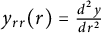 $y_{rr}(r)=\frac {d^{2}y}{dr^{2}}$
, and so on. In the paper [Reference Drugan, Lee and WheelerDLW], Drugan, Lee, and Wheeler stated the existence and asymptotic behavior of hypercylinder expanders which are homothetic soliton for the inverse mean curvature flow with
 $\lambda>1/n$
. However, there is no proof of the existence result in that paper except for the case
 $\lambda =\frac {1}{n-1}$
and the proof of the asymptotic behavior of hypercylinder expanders there are very sketchy. In this paper, I will give a new proof of the existence of hypercylinder expanders for the inverse mean curvature flow with
 $\lambda>\frac {1}{n-1}$
. We will also give a new proof of the asymptotic behavior of these hypercylinder expanders.
More precisely, I will prove the following main results.
Theorem 1.1 For any
 $n\ge 2$
,
 $\lambda>\frac {1}{n-1}$
, and
 $\mu>0$
, there exists a unique even solution
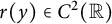 $r(y)\in C^2({{\mathbb R}})$
of the equation
 $$ \begin{align} \left\{\begin{aligned} &\frac{r^{\prime\prime}(y)}{1+r^{\prime}(y)^2}=\frac{n-1}{r(y)}-\frac{1+r^{\prime}(y)^2}{\lambda(r(y)-yr^{\prime}(y))}\,\,\,,\quad r(y)>0,\quad\forall y\in{{\mathbb R}},\\ &r(0)=\mu,\quad r^{\prime}(0)=0,\end{aligned}\right. \end{align} $$
which satisfies
 $$ \begin{align} r(y)>yr^{\prime}(y)\quad\forall y\in{{\mathbb R}} \end{align} $$
and
 $$ \begin{align} r^{\prime\prime}(0)=\left(n-1-\frac{1}{\lambda}\right)\frac{1}{\mu}. \end{align} $$
Theorem 1.2 (cf. Theorem 20 of [Reference Drugan, Lee and WheelerDLW])
Let
 $n\ge 2$
,
 $\lambda>\frac {1}{n-1}$
,
 $\mu>0$
, and
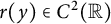 $r(y)\in C^2({{\mathbb R}})$
be the unique solution of (
1.4
). Then,
 $$ \begin{align} r^{\prime}(y)>0\quad\forall y>0, \end{align} $$
 $$ \begin{align} a_1:=\lim_{y\to\infty}r^{\prime}(y)\quad\mbox{ exists and }0\le a_1<\infty, \end{align} $$
and
 $$ \begin{align} \lim_{y\to\pm\infty}r(y)=\infty. \end{align} $$
Moreover, there exists a constant
 $y_1>0$
such that
 $$ \begin{align} \left\{\begin{aligned} &r^{\prime\prime}(y)>0\quad\forall 0<y<y_1,\\ &r^{\prime\prime}(y)<0\quad\forall y>y_1,\\ &r^{\prime\prime}(y_1)=0.\end{aligned}\right. \end{align} $$
Because (1.4) is invariant under reflection
 $y\to -y$
, by uniqueness of solution of ODE, the solution of (1.4) is an even function, and Theorem 1.1 is equivalent to the following theorem.
Theorem 1.3 For any
 $n\ge 2$
,
 $\lambda>\frac {1}{n-1}$
, and
 $\mu>0$
, there exists a unique solution
 $r(y)\in C^{2}([0,\infty ))$
of the equation
 $$ \begin{align} \left\{\begin{aligned} &\frac{r^{\prime\prime}}{1+r^{\prime}{}^{2}}=\frac{n-1}{r}-\frac{1+r^{\prime}{}^{2}}{\lambda(r-yr^{\prime})},\quad r(y)>0,\quad\forall y>0,\\ &r(0)=\mu,\quad r^{\prime}(0)=0,\end{aligned}\right. \end{align} $$
which satisfies
 $$ \begin{align} r(y)>yr^{\prime}(y)\quad\forall y>0 \end{align} $$
and ( 1.6 ).
2 Existence and asymptotic behavior of solution
In this section, we will prove Theorems 1.2 and 1.3. We first start with two lemmas which follow by standard ODE theory and Picard’s theorem.
Lemma 2.1 For any
 $n\ge 2$
,
 $\lambda \ne 0$
, and
 $\mu>0$
, there exists a constant
 $y_{0}>0$
such that the equation
 $$ \begin{align} \left\{\begin{aligned} &\frac{r^{\prime\prime}}{1+r^{\prime}{}^{2}}=\frac{n-1}{r}-\frac{1+r^{\prime}{}^{2}}{\lambda(r-yr^{\prime})}\,\,\,,\quad r(y)>0,\quad\mbox{ in }[0,y_{0})\\ &r(0)=\mu,\quad r^{\prime}(0)=0\end{aligned}\right. \end{align} $$
has a unique solution
 $r(y)\in C^{2}([0,y_{0}))$
which satisfies
 $$ \begin{align} r(y)>yr^{\prime}(y)\quad\mbox{ in }[0,y_{0}). \end{align} $$
Moreover, ( 1.6 ) holds.
Lemma 2.2 For any
 $n\ge 2$
,
 $\lambda \ne 0$
,
 $\mu>0$
,
 $M_{1}>0$
,
 $\delta _{0}>0$
,
 $r_{0},r_{1}\in {\mathbb R}$
, satisfying
 $$ \begin{align*} \delta_{0}\le r_{0}\le M_{1},\quad|r_{1}|\le M_{1},\quad r_{0}-y_{1}r_{1}\ge\delta_{0}, \end{align*} $$
there exists a constant
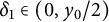 $\delta _{1}\in (0,y_{0}/2)$
depending on
 $\lambda $
,
 $\delta _{0}$
,
 $y_{0}$
, and
 $M_{1}$
such that, for any
 $y_{0}/2<y_{1}<y_{0}$
, the equation
 $$ \begin{align} \left\{\begin{aligned} &\frac{r^{\prime\prime}}{1+r^{\prime}{}^{2}}=\frac{n-1}{r}-\frac{1+r^{\prime}{}^{2}}{\lambda(r-yr^{\prime})}\,\,\,,\quad r(y)>0,\quad\mbox{ in }[y_{1},y_{1}+\delta_{1})\\ &r(y_{1})=r_{0},\quad r^{\prime}(y_{1})=r_{1}\end{aligned}\right. \end{align} $$
has a unique solution
 $r(y)\in C^{2}([y_{1},y_{1}+\delta _{1}))$
which satisfies
 $$ \begin{align} r(y)>yr^{\prime}(y)\quad\mbox{ in }[y_{1},y_{1}+\delta_{1}). \end{align} $$
Lemma 2.3 Let
 $n\ge 2$
,
 $0<\lambda \ne \frac {1}{n-1}$
,
 $\mu>0$
, and
 $y_{0}>0$
. Suppose
 $r(y)\in C^{2}([0,y_{0}))$
is the solution of (
2.1
) which satisfies (
2.2
). Then, the following holds.
-
(i) If
 $\lambda>\frac {1}{n-1}$
, then
$$ \begin{align*} r^{\prime}(y)>0\quad\forall 0<y<y_{0}. \end{align*} $$
-
(ii) If
$0<\lambda <\frac {1}{n-1}$
, then
$$ \begin{align*} r^{\prime}(y)<0\quad\quad\forall 0<y<y_{0}. \end{align*} $$




Proof. By Lemma 2.1, (1.6) holds. We divide the proof into two cases:
Case 1:
 $\lambda>\frac {1}{n-1}$
.
By (1.6),
 $r^{\prime \prime }(0)>0$
. Hence, there exists a constant
 $\delta>0$
such that
 $r^{\prime }(s)>0$
for any
 $0<s<\delta $
. Let
 $(0,a_{1})$
,
 $\delta \le a_{1}\le y_{0}$
, be the maximal interval such that
 $$ \begin{align*} r^{\prime}(s)>0\quad\forall 0<s<a_{1}. \end{align*} $$
Suppose
 $a_{1}<y_{0}$
. Then,
 $r^{\prime }(a_{1})=0$
and hence
 $r^{\prime \prime }(a_{1})\le 0$
. On the other hand, by (2.1),
 $$ \begin{align*} r^{\prime\prime}(a_{1})=\left(n-1-\frac{1}{\lambda}\right)\frac{1}{r(a_{1})}>0, \end{align*} $$
and contradiction arises. Hence,
 $a_{1}=y_{0}$
and (i) follows.
Case 2:
 $0<\lambda <\frac {1}{n-1}$
.
By (1.6),
 $r^{\prime \prime }(0)<0$
. Hence, there exists a constant
 $\delta>0$
such that
 $r^{\prime }(s)<0$
for any
 $0<s<\delta $
. Let
 $(0,a_{1})$
,
 $\delta \le a_{1}\le y_{0}$
, be the maximal interval such that
 $$ \begin{align*} r^{\prime}(s)<0\quad\forall 0<s<a_{1}. \end{align*} $$
Suppose
 $a_{1}<y_{0}$
. Then,
 $r^{\prime }(a_{1})=0$
and hence
 $r^{\prime \prime }(a_{1})\ge 0$
. On the other hand, by (2.1),
 $$ \begin{align*} r^{\prime\prime}(a_{1})=\left(n-1-\frac{1}{\lambda}\right)\frac{1}{r(a_{1})}<0, \end{align*} $$
and contradiction arises. Hence,
 $a_{1}=y_{0}$
and (ii) follows.▪
Remark 2.4 Note that if
 $r(y)$
is the local solution of (2.1) in
 $(0,y_{0})$
, it is possible that
 $$ \begin{align*} \lim_{y\to y_{0}}(r(y)-yr^{\prime}(y))=0 \end{align*} $$
or
 $$ \begin{align*} \lim_{y\to y_{0}}r^{\prime}(y)=\infty \end{align*} $$
or
 $$ \begin{align*} \lim_{y\to y_{0}}r(y)=\infty, \end{align*} $$
so that the local solution
 $r(y)$
of (2.1) cannot be continued beyond
 $y_{0}$
by standard ODE technique. Hence, in order to proof the global existence of solution of (1.11), we need the following two lemmas which show that this cannot happen.
Lemma 2.5 Let
 $n\ge 2$
,
 $\lambda>\frac {1}{n-1}$
,
 $\mu>0$
, and
 $y_{0}>0$
. Suppose
 $r(y)\in C^{2}([0,y_{0}))$
is the solution of (
2.1
) which satisfies (
2.2
). Then, there exist a constant
 $\delta _{1}>0$
such that
 $$ \begin{align} r(y)-yr^{\prime}(y)\ge\delta_{1}\quad\forall 0<y<y_{0}. \end{align} $$
Proof. Let
 $w(y)=r(y)-yr^{\prime }(y)$
,
 $a_{1}=\min _{0\le y\le y_{0}/2}w(y)$
,
 $a_{2}=\frac {\mu }{\lambda (n-1)}$
, and
 $a_{3}=\frac {1}{2}\min (a_{1},a_{2})$
. Then,
 $a_{1}>0$
and
 $a_{3}>0$
. By Lemma 2.3,
 $$ \begin{align} r(y)\ge\mu\quad\forall 0<y<y_{0}. \end{align} $$
Suppose there exists
 $y_{1}\in (y_{0}/2,y_{0})$
such that
 $w(y_{1})<a_{3}$
. Let
 $(a,b)$
be the maximal interval containing
 $y_{1}$
such that
 $w(y)<a_{3}$
for any
 $y\in (a,b)$
. Then,
 $a>y_{0}/2$
,
 $w(a)=a_{3}$
, and
 $$ \begin{align} w(y)<\frac{\mu}{2\lambda(n-1)}\quad\forall a<y<b. \end{align} $$
By (2.1), (2.6), (2.7), and a direct computation,
 $$ \begin{align*} w^{\prime}(y)=&\,y(1+r^{\prime}(y)^{2})\left(\frac{1+r^{\prime}(y)^{2}}{\lambda w(y)}-\frac{n-1}{r(y)}\right)\quad\forall 0<y<y_{0}\nonumber\\ \ge&\,y(1+r^{\prime}(y)^{2})\left(\frac{1}{2\lambda w(y)}+\left(\frac{1}{2\lambda w(y)}-\frac{n-1}{\mu}\right)\right)\quad\forall a<y<b\nonumber\\ \ge&\,\frac{y_{0}}{4\lambda w(y)}>0\quad\forall a<y<b.\nonumber \end{align*} $$
Hence,
 $$ \begin{align*} w(y)>w(a)=a_{3}\quad\forall a<y<b, \end{align*} $$
and contradiction arises. Hence, no such
 $y_{1}$
exists, and
 $w(y)\ge a_{3}$
for any
 $y\in (0,y_{0})$
. Thus, (2.5) holds with
 $\delta _{1}=a_{3}$
.▪
Lemma 2.6 Let
 $n\ge 2$
,
 $\lambda>\frac {1}{n-1}$
,
 $\mu>0$
, and
 $y_{0}>0$
. Suppose
 $r(y)\in C^{2}([0,y_{0}))$
is the solution of (
2.1
) which satisfies (
2.2
). Then, there exists a constant
 $M_{1}>0$
such that
 $$ \begin{align} 0<r^{\prime}(y)\le M_{1}\qquad\forall 0<y<y_{0} \end{align} $$
and
 $$ \begin{align} \mu\le r(y)\le \mu+M_{1}y_{0}\quad\forall 0<y<y_{0}. \end{align} $$
Proof. By (2.1), (2.2), and Lemma 2.3,
 $$ \begin{align} \frac{r^{\prime\prime}}{1+r^{\prime}{}^{2}}\le\frac{n-1}{r}\le\frac{n-1}{\mu}\quad\forall 0<y<y_{0}. \end{align} $$
Integrating (2.10) over
 $(0,y_{0})$
,
 $$ \begin{align} \tan^{-1}(r^{\prime}(y))\le\frac{(n-1)y_{0}}{\mu}\quad\forall 0<y<y_{0}. \end{align} $$
By Lemma 2.3 and (2.11), (2.8) holds with
 $$ \begin{align*} M_{1}=\tan\left(\frac{(n-1)y_{0}}{\mu}\right). \end{align*} $$
Lemma 2.7 Let
 $n\ge 2$
,
 $\lambda>\frac {1}{n-1}$
,
 $\mu>0$
, and
 $y_{0}>0$
. Suppose
 $r(y)\in C^{2}([0,y_{0}))$
is the solution of (
2.1
) which satisfies (
2.2
). Then, either
 $$ \begin{align} r^{\prime\prime}(y)>0\quad\forall 0<y<y_{0}, \end{align} $$
or there exists a constant
 $y_{1}\in (0,y_{0})$
such that
 $r^{\prime \prime }(y_{1})=0$
and
 $$ \begin{align} \left\{\begin{aligned} &r^{\prime\prime}(y)>0\quad\forall 0<y<y_{1},\\ &r^{\prime\prime}(y)<0\quad\forall y_{1}<y<y_{0}. \end{aligned}\right. \end{align} $$
Proof. We will use a modification of the proof of Lemma 15 of [Reference Drugan, Lee and WheelerDLW] to prove this lemma. By (1.6),
 $r^{\prime \prime }(0)>0$
. Hence, there exists a constant
 $\delta>0$
such that
 $r^{\prime \prime }(s)>0$
for any
 $0<s<\delta $
. Let
 $(0,y_{1})$
,
 $\delta \le y_{1}\le y_{0}$
, be the maximal interval such that
 $$ \begin{align*} r^{\prime\prime}(s)>0\quad\forall 0<s<y_{1}. \end{align*} $$
If
 $y_{1}=y_{0}$
, then (2.12) holds. If
 $y_{1}<y_{0}$
, then
 $r^{\prime \prime }(y_{1})=0$
. By Lemma 2.3 and (2.1),
 $$ \begin{align} \frac{r^{\prime\prime\prime}(y)}{1+r^{\prime}(y)^{2}}=&\frac{2r^{\prime}(y)r^{\prime\prime}(y)^{2}}{(1+r^{\prime}(y)^{2})^{2}}-\frac{n-1}{r(y)^{2}}r^{\prime}(y)-\frac{2r^{\prime}(y)r^{\prime\prime}(y)}{\lambda(r(y)-yr^{\prime}(y))}\nonumber\\[4pt] &\quad -\frac{y(1+r^{\prime}(y)^{2})r^{\prime\prime}(y)}{\lambda(r(y)-yr^{\prime}(y))^{2}}\,\forall 0<y<y_{0}\\[4pt] \Rightarrow\,\frac{r^{\prime\prime\prime}(y_{1})}{1+r^{\prime}(y_{1})^{2}}=&-(n-1)\frac{r^{\prime}(y_{1})}{r(y_{1})^{2}}<0.\nonumber \end{align} $$
Hence, there exists a constant
 $0<\delta ^{\prime }<y_{0}-y_{1}$
such that
 $r^{\prime \prime }(y)<0$
for any
 $y_{1}<y<y_{1}+\delta ^{\prime }$
. Let
 $(y_{1},z_{0})$
be the maximal interval such that
 $$ \begin{align*} r^{\prime\prime}(s)<0\quad\forall y_{1}<s<z_{0}. \end{align*} $$
If
 $z_{0}<y_{0}$
, then
 $r^{\prime \prime }(z_{0})=0$
and
 $r^{\prime \prime }(z_{0})\ge 0$
. On the other hand, by Lemma 2.3 and (2.14),
 $$ \begin{align*} \frac{r^{\prime\prime\prime}(z_{0})}{1+r^{\prime}(z_{0})^{2}}=-(n-1)\frac{r^{\prime}(z_{0})}{r(z_{0})^{2}}<0, \end{align*} $$
and contradiction arises. Hence,
 $z_{0}=y_{0}$
and (2.13) follows.▪
We are now ready to prove Theorem 1.3.
2.1 Proof of Theorem 1.3
By Lemma 2.1, there exists a constant
 $y_{0}^{\prime }>0$
such that (2.1) has a unique solution
 $r(y)\in C^{2}([0,y_{0}^{\prime }))$
which satisfies (1.6) and (2.2) in
 $(0,y_{0}^{\prime })$
. Let
 $(0,y_{0})$
be the maximal interval of existence of solution
 $r(y)\in C^{2}([0,y_{0}))$
of (2.1) which satisfies (2.2) and (1.6). Suppose
 $y_{0}<\infty $
. By Lemmas 2.2, 2.5, and 2.6, there exists a constant
 $\delta _{1}\in (0,y_{0})$
such that, for any
 $y_{0}/2<y_{1}<y_{0}$
, there exists a unique solution
 $r_{1}(y)\in C^{2}([y_{1},y_{1}+\delta _{1}))$
of (2.3) which satisfies (2.4) with
 $r_{0}=r(y_{1})$
and
 $r_{1}=r^{\prime }(y_{1})$
. Let
 $y_{1}\in \left (y_{0}-\frac {\delta _{1}}{2},y_{0}\right )$
, and let
 $r_{1}(y)\in C^{2}([y_{1},y_{1}+\delta _{1}))$
be the unique solution of (2.3) given by Lemma 2.2 which satisfies (2.4) with
 $r_{0}=r(y_{1})$
and
 $r_{1}=r^{\prime }(y_{1})$
. We then extend
 $r(y)$
to a solution of (1.11) in
 $(0,y_{1}+\delta _{1})$
by setting
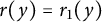 $r(y)=r_{1}(y)$
for any
 $y_{0}\le y<y_{1}+\delta _{1}$
. Because
 $y_{1}+\delta _{1}>y_{0}$
, this contradicts the maximality of the interval
 $(0,y_{0})$
. Hence,
 $y_{0}=\infty $
, and there exists a unique solution
 $r(y)\in C^{2}([0,\infty ))$
of the equation (1.11) which satisfies (1.12) and (1.6) and the theorem follows.
 $\square $
2.2 Proof of Theorem 1.2
We will give a simple proof different from the sketchy proof of this result in [Reference Drugan, Lee and WheelerDLW] here. By (i) of Lemma 2.3, (1.7) holds. By Lemma 2.7, either
 $$ \begin{align} r^{\prime\prime}(y)>0\quad\forall y>0, \end{align} $$
or there exists
 $y_{1}>0$
such that (1.10) holds. Suppose (2.15) holds. Then,
 $$ \begin{align} a_{1}:=\lim_{y\to\infty}r^{\prime}(y)\quad\mbox{ exists, } \end{align} $$
and
 $a_{1}>0$
. We now divide the proof into two cases.
Case 1:
 $a_{1}=\infty $
.
Then, there exists
 $y_{2}>0$
such that
 $$ \begin{align} r^{\prime}(y)>\sqrt{2(n-1)\lambda}\quad\forall y>y_{2}. \end{align} $$
 $$ \begin{align*} \frac{r^{\prime\prime}(y)}{1+r^{\prime}(y)^{2}}\le&\frac{1}{r(y)}\left(n-1-\frac{1+r^{\prime}(y)^{2}}{\lambda}\right)\qquad\qquad\,\,\forall y>0\nonumber\\ \le&\frac{1}{r(y)}\left(n-1-\frac{1+2(n-1)\lambda}{\lambda}\right)<0\quad\forall y>y_{2}, \end{align*} $$
which contradicts (2.15). Hence,
 $a_{1}\ne \infty $
.
Case 2:
 $a_{1}<\infty $
.
By (1.12),
 $$ \begin{align} 0<\frac{yr^{\prime}(y)}{r(y)}<1\quad\forall y>0. \end{align} $$
Now, by (2.16) and the l’Hosiptal rule,
 $$ \begin{align} \lim_{y\to\infty}\frac{r(y)}{y}=\lim_{y\to\infty}r^{\prime}(y)=a_{1}\quad \Rightarrow\quad\lim_{y\to\infty}\frac{yr^{\prime}(y)}{r(y)}=\frac{\lim_{y\to\infty}r^{\prime}(y)}{\lim_{y\to\infty}r(y)/y}=1. \end{align} $$
By (1.11), (2.16), (2.18), (2.19), and the l’Hosiptal rule,
 $$ \begin{align*} \lim_{y\to\infty}\frac{r(y)r^{\prime\prime}(y)}{1+a_{1}^{2}} =&\lim_{y\to\infty}\frac{r(y)r^{\prime\prime}(y)}{1+r^{\prime}(y)^{2}}\nonumber\\ =&n-1-\frac{1+a_{1}^{2}}{\lambda}\cdot\frac{1}{\lim_{y\to\infty}\left(1-\frac{yr^{\prime}(y)}{r(y)}\right)}\nonumber\\ =&-\infty, \end{align*} $$
which contradicts (2.15). Hence,
 $a_{1}<\infty $
does not hold. Thus, by Cases 1 and 2, (2.15) cannot hold. Hence, there exists
 $y_{1}>0$
such that (1.10) holds.
By (1.10) and Lemma 2.3, (1.8) holds. By (1.7),
 $$ \begin{align*} a_{2}:=\lim_{y\to\infty}r(y)\in (\mu,\infty]\quad\mbox{ exists}. \end{align*} $$
Because by (1.10)
 $(r(y)-yr^{\prime }(y))^{\prime }=-yr^{\prime \prime }(y)>0$
for any
 $y>y_{1}$
,
 $$ \begin{align} a_{3}:=\lim_{y\to\infty}(r(y)-yr^{\prime}(y))\in (r(y_{1})-y_{1}r^{\prime}(y_{1}),\infty]\quad\mbox{ exists}. \end{align} $$
Suppose
 $$ \begin{align} a_{2}\in (\mu,\infty). \end{align} $$
Then,
 $$ \begin{align} a_{1}=0. \end{align} $$
 $$ \begin{align*} a_{4}:=\lim_{y\to\infty}yr^{\prime}(y)=a_{2}-a_{3}\in [0,a_{2}-r(y_{1})+y_{1}r^{\prime}(y_{1}))\quad\mbox{ exists}. \end{align*} $$
Suppose
 $a_{4}>0$
. Then, there exists
 $y_{2}>y_{1}$
such that
 $$ \begin{align*} yr^{\prime}(y)\ge &a_{4}/2\quad\forall y\ge y_{2}\\ \Rightarrow\qquad\,\, r(y)\ge& r(y_{2})+\frac{a_{4}}{2}\log (y/y_{2})\quad\forall y\ge y_{2}\\ \Rightarrow\qquad\quad a_{2}= &\infty, \end{align*} $$
which contradicts (2.21). Hence,
 $$ \begin{align} a_{4}=0. \end{align} $$
Letting
 $y\to \infty $
in (1.11), by (2.22) and (2.23),
 $$ \begin{align*} \lim_{y\to\infty}r^{\prime\prime}(y)=\left(n-1-\frac{1}{\lambda}\right)\frac{1}{a_{2}}>0, \end{align*} $$
which contradicts (1.10). Hence, (2.21) does not hold and
 $a_{2}=\infty $
. Thus, (1.9) holds and the theorem follows.
Acknowledgment
The author would like to thank the anonymous referee for the numerous helpful and detailed comments on the paper.


