

1. Introduction
Particle-laden flows – owing to the abundance of applications in which they are encountered including sand storms (Kok et al. Reference Kok, Parteli, Michaels and Karam2012), soot emissions (Malmborg et al. Reference Malmborg, Eriksson, Shen, Nilsson, Gallo, Waldheim, Martinsson, Andersson and Pagels2017) and fluidized beds (Cocco, Karri & Knowlton Reference Cocco, Karri and Knowlton2014) – have garnered considerable interest in the scientific community. Particle-laden flows are often studied via Euler–Lagrangian (EL) simulation. In EL methods, partial differential equations (such as mass, momentum, temperature, electric field) for the fluid or carrier phase are discretized in space while ordinary differential equations (such as position, momentum, temperature and charge) governing the particle or dispersed phase are solved along Lagrangian trajectories for each particle. EL methods are closed by assuming models for how the particles will interact with the fluid and with each other. One-way coupled EL methods describe models whereby particle quantities (position/momentum etc.) are influenced by the surrounding fluid environment, but fluid quantities (velocity, temperature) feel no effect from the particles. In two-way coupled approaches, particles are influenced by the surrounding fluid fields, and the fluid fields themselves are influenced by the particles. This can happen, for example, when a hot particle is placed in a cold surrounding fluid. A two-way coupled EL approach will model how the particle will cool down and how the fluid will heat up (Horwitz et al. Reference Horwitz, Ganguli, Mani and Lele2017; Liu, Lakhote & Balachandar Reference Liu, Lakhote and Balachandar2019). In four-way coupled EL methods, in addition to the mutual interaction of particles and fluid, explicit models are used to account for the mutual influence between particles. Mutual interactions between particles include collisions which cause a change in momentum (Cundall & Strack Reference Cundall and Strack1979) and charge (Yao & Capecelatro Reference Yao and Capecelatro2018), depending on the application, of the colliding particles. Lubrication and multi-particle hydrodynamic interactions can also be modelled analytically through mobility functions (Kim & Karrila Reference Kim and Karrila2005) or numerically using approaches like the pairwise interaction extended point-particle (PIEP) method (Akiki, Jackson & Balachandar Reference Akiki, Jackson and Balachandar2017).
In this work, we are concerned principally with issues that arise in two-way coupled EL methods. Hereafter, the primary focus will be on dilute gas–solid flows where the density ratio between dispersed and carrier phase is significant yet the volume fraction is small. This will allow us to neglect particle-neighbour effects to first order and consider quasi-steady drag for particle motion. To elucidate the challenge, let us consider only hydrodynamic interactions between a fluid and a single rigid spherical particle. When the flow is steady and the particle Reynolds number  $Re_{p} = |\tilde {\boldsymbol {u}}-\boldsymbol {v_p}|d_p/\nu \ll 1$, the interaction between the fluid and particle is well described by the Stokes drag force
 $\boldsymbol {f_d} = 3{\rm \pi} \mu d_p (\tilde {\boldsymbol {u}}-\boldsymbol {v_p})$. Here,
 $\boldsymbol {v_p}$ and
 $d_p$ are respectively the particle velocity and diameter,
 $\mu$ and
 $\nu$ are respectively the fluid dynamic and kinematic viscosity and
 $\tilde {\boldsymbol {u}}$ is the undisturbed fluid velocity centred at the particle position (Maxey & Riley Reference Maxey and Riley1983). In a two-way coupled EL simulation, this Stokes drag force felt by the particle models the rate of change of momentum deficit in the fluid. The momentum deficit in the fluid is characterized by a disturbance flow created by and typically occurring in the near field of the particle. This disturbance flow contaminates the surrounding fluid so that the undisturbed state prior to the introduction of the particle is no longer available. In other words, it is not possible to calculate
 $\tilde {\boldsymbol {u}}$, which is needed to compute the drag force, changing the motion of the particle, and the fluid velocity, as the simulation is being performed. This observation has been the subject of considerable research in recent years.
Within the past five years, several methods have been proposed to estimate the undisturbed fluid velocity for momentum two-way coupled EL methods (Gualtieri et al. Reference Gualtieri, Picano, Sardina and Casciola2015; Horwitz & Mani Reference Horwitz and Mani2016; Ireland & Desjardins Reference Ireland and Desjardins2017; Esmaily & Horwitz Reference Esmaily and Horwitz2018; Horwitz & Mani Reference Horwitz and Mani2018; Balachandar, Liu & Lakhote Reference Balachandar, Liu and Lakhote2019; Fukada, Takeuchi & Kajishima Reference Fukada, Takeuchi and Kajishima2019; Poustis et al. Reference Poustis, Senoner, Zuzio and Villedieu2019) as well as the undisturbed temperature for thermally two-way coupled EL methods (Horwitz et al. Reference Horwitz, Ganguli, Mani and Lele2017; Liu et al. Reference Liu, Lakhote and Balachandar2019). These methods have shown similar accuracy in the context of laminar verification problems while they have different ranges of applicability. Some of these methods are properly suited for low particle Reynolds number (Gualtieri et al. Reference Gualtieri, Picano, Sardina and Casciola2015; Horwitz & Mani Reference Horwitz and Mani2016; Ireland & Desjardins Reference Ireland and Desjardins2017) while others have been extended to finite Reynolds number (Esmaily & Horwitz Reference Esmaily and Horwitz2018; Horwitz & Mani Reference Horwitz and Mani2018; Balachandar et al. Reference Balachandar, Liu and Lakhote2019; Fukada et al. Reference Fukada, Takeuchi and Kajishima2019; Poustis et al. Reference Poustis, Senoner, Zuzio and Villedieu2019). While some methods are suited to isotropic grids (Horwitz & Mani Reference Horwitz and Mani2016, Reference Horwitz and Mani2018; Horwitz et al. Reference Horwitz, Ganguli, Mani and Lele2017), other methods can be employed on more general grid configurations (Gualtieri et al. Reference Gualtieri, Picano, Sardina and Casciola2015; Ireland & Desjardins Reference Ireland and Desjardins2017; Esmaily & Horwitz Reference Esmaily and Horwitz2018; Balachandar et al. Reference Balachandar, Liu and Lakhote2019; Liu et al. Reference Liu, Lakhote and Balachandar2019; Poustis et al. Reference Poustis, Senoner, Zuzio and Villedieu2019). A summary of these methods is presented in table 1. Besides which drag correlation and what type of mesh structure these methods are suited to, one area that has not received attention in the literature is the manner in which the domain and discretization of the field equations contribute to how the undisturbed fluid velocity should be estimated. These previous methods implicitly assume the fluid domains have homogeneous or periodic boundary conditions. When the boundary conditions become more complicated, for example when one or more no-slip/no-penetration walls is introduced, these methods are no longer strictly valid. An inherent assumption is that the disturbance flow created by a particle can freely decay. In the language we will adopt in the next section, these methods assume the disturbance flow to be given by the discrete Green's function (DGF) response in an unbounded domain. At large distances, this will go like the inverse radial distance from the particle centre  $\sim 1/r$, or the asymptotic form of the continuous Stokeslet or Green's function of the Stokes equations. When a particle moves near a wall, especially at close distances, the disturbance flow the particle creates must be damped by the wall to satisfy the no-slip/no-penetration condition (Blake & Chwang Reference Blake and Chwang1974; Liron & Mochon Reference Liron and Mochon1976). None of the aforementioned methods explicitly account for the presence of the wall. While several of the previous methods are suited to anisotropic grids which are common in the simulation of wall-bounded flows, we will show in the verification section that capturing the wall-damping effect is essential to accurately computing the two-way coupling force. We will also demonstrate explicitly how discretization of the field equations (via finite differences or finite elements for example) is connected to the discrete disturbance flow and ultimately the computation of the undisturbed fluid velocity. It is worth mentioning that the exact regularized point-particle method (ERPP) (Gualtieri et al. Reference Gualtieri, Picano, Sardina and Casciola2015) was recently extended to the wall-bounded flow regime (Battista et al. Reference Battista, Mollicone, Gualtieri, Messina and Casciola2019). This approach is particularly attractive in its incorporation of unsteady effects, however, ERPP is presently limited to low particle Reynolds number, which will not be a general limitation of the method presented in this work. In concluding this literature review, there is much work being done to develop methods to estimate undisturbed quantities in a variety of scenarios (momentum/heat transfer, quasi-steady/unsteady sources, unbounded/wall-bounded flows etc.) and this paper is among those efforts to propose remedies to this computational challenge as well as elucidate deeper understanding of this problem.
Different methods to compute the undisturbed velocity (momentum coupling) or temperature (thermal coupling). Interpolation refers to data transfer from fluid to particle, while projection refers to transfer from particle to fluid. ‘General’/‘Anisotropic’ refer to the fact that those particular methods may be suitable to a wider range of interpolation stencils and mesh configurations than specifically tested in those works.

The remainder of the paper is broken into five parts. The first section demonstrates the relationship between the discretized fluid field equations and discrete Green's functions, as well as how the discrete Green's function can be used to estimate the undisturbed fluid velocity. The next section discusses the procedure for finding discrete Green's functions. We apply this procedure to obtain the discrete Green's functions to the Stokes equations in a two-plane channel geometry. In the third section, we present a set of verification exercises where a particle settles under gravity moving parallel to a plane wall. We repeat this exercise for different wall-normal separations, particle Reynolds numbers and methods to compute the undisturbed fluid velocity. In the penultimate section, we consider a turbulent particle-laden channel flow to understand what role the manner of calculating the undisturbed fluid velocity plays in the turbulence statistics. Concluding remarks are given in the final section.
2. Origin of discrete Green's functions
In this section, we demonstrate the connection between discretized partial differential equations (PDEs) and their associated discrete Green's function. We will focus our attention on the discrete Stokes equations. However, it is worth noting that the method of discrete Green's functions applies to a much larger class of problems. Malgrange (Reference Malgrange1956) and Ehrenpreis (Reference Ehrenpreis1954) proved that every linear PDE with constant coefficients admits a Green's function. Zeilberger (Reference Zeilberger2011) later showed every linear constant coefficient PDE has a discrete Green's function. While Lewy's example (Lewy Reference Lewy1957) demonstrates that not all non-constant coefficient linear PDEs have a solution, there still exist linear non-constant coefficient PDEs which have Green's functions, e.g. the spherically symmetric wave (Haberman Reference Haberman2004) and heat (Hahn & Ozisik Reference Hahn and Ozisik2012) equations. Therefore, while we focus on the Stokes equations in this section, the same manipulations can be readily performed for the thermal energy or Maxwell's equations, e.g. written in Cartesian or other coordinate systems, as the application demands.
Let us consider now the steady Stokes equations, understood as the regular limit of the Navier–Stokes equations as the Reynolds number goes to zero, subject to a point-force density
 $$\begin{gather} \mu\frac{\partial^2 u_i}{\partial x_j\partial x_j}-\frac{\partial p}{\partial x_i}= F_{i}, \end{gather}$$
 $$\begin{gather}\frac{\partial^2 p}{\partial x_j\partial x_j} ={-}\frac{\partial F_i}{\partial x_i}. \end{gather}$$
In the above,  $u_i$ and
 $p$ are respectively the fluid velocity and pressure, and
 $F_i$ is a force density applied at the particle centre owing to two-way coupling. Let us consider a spatial discretization of the above system
 $$\begin{gather} \mu\frac{\delta^2u_i^n}{\delta x_j \delta x_j}-\frac{\delta p^n}{\delta x_i}= F_{i}^n, \end{gather}$$
 $$\begin{gather}\frac{\delta^2 p^n}{\delta x_j \delta x_j} ={-}\frac{\delta F_i^n}{\delta x_i}. \end{gather}$$
Here, the superscript  $n$ denotes a field variable evaluated at grid point
 $n$ and
 ${\delta }/{\delta x_i}$ is the discrete differential operator associated with the continuous differential operator
 ${\partial }/{\partial x_i}$. By introducing the following discrete differential operators:
 $C^{kn} \equiv (\nabla ^2)^{-1}$,
 $A_j()_j\equiv ({\partial }/{\partial x_j})()_j$, and
 $B_{i} =\boldsymbol {\nabla }$, we can write the formal solution to (2.3) and (2.4) as (this discrete pressure solution is not unique since the uniform background pressure is arbitrary, however, the discrete pressure gradient which is present in (2.3) is unique)
 $$\begin{gather} p^k ={-}C^{kn}A_jF_j^n, \end{gather}$$
 $$\begin{gather}u_i^n = \mu^{{-}1}C^{nk}(\delta_{ij}^{kp}-B_iC^{kp}A_j)F_j^p. \end{gather}$$
By letting  $G_{ij}^{np} = \mu ^{-1}C^{nk}(\delta _{ij}^{kp}-B_iC^{kp}A_j)$, (2.6) can be written in a simpler form
 \begin{equation} u_i^n = G_{ij}^{np}F_j^p. \end{equation}
In (2.7),  $G_{ij}^{np}$ is called the discrete Green's function associated with the discrete Stokes equations. This discrete Green's function provides a mapping of a discrete point force at grid point
 $p$ in direction
 $j$ to a discrete disturbance flow at grid point
 $n$ in direction
 $i$. Here, we have made no assumption regarding the imposed boundary conditions (homogeneous or wall bounded for example), grid structure (uniform/non-uniform/unstructured) or discretization scheme (second- vs fourth-order finite differences, or spectral for example). In other words, there exists in general a different discrete Green's function for each discrete PDE, for each set of boundary conditions, grid structure and discretization scheme.
Our focus is not on exploring the sensitivity to each of these parameters but on elucidating how the discrete Green's function can be used to estimate undisturbed field quantities. In EL simulation, the force that a particle experiences  $f_{i}$ is transferred from the Lagrangian particle to Eulerian discrete grid points via a projection operator, often via a Gaussian, Lagrange polynomial or spline function. Dividing by the volume of the fluid element yields the discrete force density
 $F_i^n$. When this discrete force density is applied to the discrete fluid equations, the fluid velocity at each grid point will change from an undisturbed state
 $\tilde {u}_i^k$ to some new fluid velocity
 $u_i^k$, such that the new fluid velocity at grid point
 $k$ can be written in the form
 $u_i^k = \tilde {u}_i^k + u^{d,k}_i$, where
 $u^{d,k}_i$ is the disturbance velocity introduced by the particle at grid point
 $k$. If the disturbance velocity were known, then it would be possible to rearrange the previous expression to compute the undisturbed fluid velocity as
 $\tilde {u}_i^k = u_i^k - u^{d,k}_i$. The undisturbed fluid velocity at the particle location could then be calculated by interpolation of the undisturbed fluid velocity from the Eulerian grid points to the particle location. Let us introduce the operators
 $W^k$ and
 $w^n$ as the weights associated with interpolation and projection, respectively. If we assume that the discrete Green's function previously introduced provides a good approximation between the discrete force density
 $F_i^n$ and discrete disturbance flow
 $u^{d,k}_i$, the undisturbed fluid velocity at the particle location can be estimated as
 \begin{equation} \tilde{u}_i \approx W^k\{u^k_i-G_{ij}^{kn} w^n f_j\}. \end{equation}
Interestingly, the undisturbed fluid velocity can be accurately estimated regardless of the choice of interpolation/projection stencil as previously alluded to in Esmaily & Horwitz (Reference Esmaily and Horwitz2018). While Gaussian schemes may offer certain advantages to stability or smoothing of the flow field near the particle (Poustis et al. Reference Poustis, Senoner, Zuzio and Villedieu2019), it seems low-memory access interpolation/projection may still be advantageous since these EL data-transfer methods still allow accurate computation of the undisturbed fluid velocity and hence the energetics of the system will be consistent with the chosen drag law (Mehrabadi et al. Reference Mehrabadi, Horwitz, Subramaniam and Mani2018; Horwitz & Mani Reference Horwitz and Mani2020). From the standpoint of storage, it may also be favourable to use low-memory access projection/interpolation stencils to reduce the cost of storing the discrete Green's function. For even a modest problem size of say  $10^{6}$ grid points, the whole discrete Green's function would involve
 $O(10^{12})$ elements for a general problem. However, if we consider only the points which will actually be accessed for computing the undisturbed fluid velocity, the
 $n$ points associated with
 $W^n$ and
 $w^n$, the result can be enormous computational savings. We will give a more precise estimate of the storage and computational cost associated with discrete Green's functions in the next section.
3. Finding discrete Green's functions
For a general problem, the discrete Green's function for the Stokes equations involves the mapping of three force components at  $N$ grid points, to three velocity components at
 $N$ grid points, so that the total size of the DGF is
 $9N^{2}$. In addition to the large memory requirements to store this object, the construction of the DGF would require solving the Stokes equations successively, in each case with a point force placed at a different grid point in a different coordinate direction. Therefore, direct computation of the DGF is infeasible for most problems. An alternative approach for general problems which relies on approximating DGFs locally is discussed in Horwitz (Reference Horwitz2018).
We consider the computation of the discrete Green's function for a two-plane channel flow geometry, a domain with considerable interest in particle-laden flow problems (Kulick, Fessler & Eaton Reference Kulick, Fessler and Eaton1994; Sardina et al. Reference Sardina, Schlatter, Brandt, Picano and Casciola2012; Costa, Brandt & Picano Reference Costa, Brandt and Picano2020). In addition, the two-plane channel geometry has two homogeneous directions which may be exploited to dramatically reduce the cost associated with computation and storage of the DGF. A diagram of the flow domain is shown in figure 1(a). The boundary conditions are periodic in the streamwise ( $x$) and spanwise (
 $z$) direction, while the velocity obeys no slip and no penetration at the top and bottom walls. Owing to the homogeneous directions (
 $x,z$), the discrete Green's function will be invariant with respect to translation in those directions. Hence, we may choose a fixed (
 $x,z$) line to consider the problem of finding the discrete Green's function for different wall-normal particle positions (figure 1(b)). Owing to symmetry about the centreplane of the channel, we need only consider one half of the channel. Therefore, to compute the whole discrete Green's function will require running
 $3N_{y}/2$ simulations of the Stokes equations in the two-plane channel geometry. By assuming the projection and interpolation operators are trilinear stencils, we will ultimately construct an object of size
 $24\times 24\times N_{y}/2$. In a trilinear stencil, eight degrees of freedom are involved for each of three velocity directions. In other words, for a given wall-normal distance a general force which may have components in the
 $x, y$ and
 $z$ directions will involve
 $24$ degrees of freedom, and will be mapped, at a given wall-normal distance, through a tensor involving
 $24\times 24 = 576$ components, to
 $24$ velocity components, eight for each of three directions. Only these
 $24\times 24$ elements must be considered for each wall-normal location because the choice of trilinear stencil to be incorporated in the interpolation/projection stencils ensures there will be no contribution to the self-disturbed fluid velocity at a given particle's location owing to distant grid points, or those outside the set of
 $24$. See figure 2 which shows a collocated grid arrangement to make the surrounding discussion more intuitive. The staggered grid implemented in the present work requires additional considerations which are discussed in Appendix D.
(a) Simulation domain and (b) depiction of the locations where point forces will be placed in order to calculate the discrete Green's functions.

Grid points involved in trilinear interpolation and projection for a collocated arrangement. For an arbitrary location of a particle in the domain, the surrounding grid points can be mapped to the notation used here. Streamwise components are denoted with  $u$, spanwise with
 $w$ and wall normal with
 $v$.

To calculate the DGFs, the Navier–Stokes equations are solved at low Reynolds number and integrated for several viscous times until the solution becomes steady. This process is repeated  $3N_y/2$ times; in each simulation, a point force of magnitude unity is placed at different grid points in the domain, one for each coordinate direction, and
 $N_y/2$ to cover all wall-normal locations. (This problem is symmetric about the channel centreplane so we need only consider half of the wall-normal grid points.) The magnitudes of the kinematic viscosity
 $\nu$ and density
 $\rho$ are chosen such that
 $f/2{\rm \pi} \rho \nu ^2 \ll 1$, so that this discrete problem represents the low Reynolds number limit of the Landau–Squire jet (Batchelor Reference Batchelor1967). The mean streamwise pressure gradient,
 $-\textrm {d}p/{\textrm {d}\kern0.7pt x}$ is set to zero, so that the resulting flow is only owing to the presence of the discrete point force. The streamwise and spanwise lengths are large enough to ensure minimal effects from the periodic boundary conditions (see the disturbance length scale in figure 3). Time advancement is accomplished with second-order Runge–Kutta. The grid arrangement is a staggered configuration (figures 1b). The grid spacing is uniform in the streamwise and spanwise directions with 96 grid points in each of those directions. The wall-normal direction uses 128 grid points in a non-uniform arrangement given by a hyperbolic tangent profile which clusters more grid points near the wall. The pressure equation is solved using multi-grid acceleration. All spatial derivatives are discretized with second-order finite differences. More details on the implementation can be found in Esmaily et al. (Reference Esmaily, Jofre, Mani and Iaccarino2018).
Profiles of streamwise velocity disturbances generated by streamwise point force placed in the (a) near wall, and (b) away from wall regions. Insets show near-field response. Notice the strong asymmetry in the streamwise response in the near-wall disturbance compared with the away-from-the-wall disturbance.

To determine the discrete Green's functions from the calculated solution, we isolate each of the elements of the DGF for each wall-normal distance. For example, the velocity disturbance for streamwise component  $1$ owing to a point force placed at component
 $1$, can be obtained as
 $G^{1,1}=u_{1}/F_{1} = u_1$ (see figure 2). Similarly, for a point force applied at
 $9$,
 $G^{9,9}$ can be calculated as
 $G^{9,9}=v_{9}/F_{9}=v_{9}$. Certain off-diagonal elements of the DGF can be directly measured using this strategy. For example, when the force is applied to
 $1$, the velocity calculated at
 $5$ corresponds to
 $G^{5,1}$. However, not all elements of the DGF can be directly calculated from the
 $3N_{y}/2$ simulations. For these remaining components of the DGF, it is necessary to exploit symmetries. For example, in practice, we only put a force at
 $1$ and not
 $2$. However, had we put a force on
 $2$, it can be observed that
 $G^{2,2}=G^{1,1}$. Stokesian symmetry can also be exploited, for example the response at
 $1$ due to a force applied to
 $4$ is the same as the response at
 $4$ due to a force at
 $1$, viz.
 $G^{1,4}=G^{4,1}$. By exploiting all such symmetries, we can fill out the DGF for a given wall-normal location. By then combining the 576 elements for each wall-normal location, we develop the complete DGF object for the channel flow. In figure 4, we plot the loci of
 $G^{1,1}$ and
 $G^{14,17}$ as functions of wall-normal distance to gain an understanding of what the DGF object looks like. We can see the magnitude of
 $G^{1,1}$ is much greater than the magnitude of
 $G^{14,17}$ over the whole of the channel. It is not surprising that the greatest response to the point force is typically at the location of application of the point force and in the same direction. There is an exception, however, with respect to the wall-normal diagonal components of the DGF. This is reflected in figure 5. Here, we have plotted all components of the DGF at two wall-normal locations, one close to the wall in figure 5(a), and one close to the centre of the channel (figure 5b). Near the wall, when a force is applied in the wall-normal direction, there is minimal response. The no-penetration condition demands the induced wall-normal response to scale as
 $y^{2}$ near the wall (Pope Reference Pope2000). In contrast, the no-slip condition demands that the streamwise and spanwise velocity disturbances vary linearly near the wall. Hence, force components in the streamwise and spanwise directions generate relatively large responses in those directions compared with the wall-normal direction. In other words, the velocity disturbance induced by an arbitrary point force near the wall is almost planar. In contrast, near the centre of the channel, the wall-damping effects are diminished, and the velocity disturbance owing to an arbitrary point force is a three-dimensional, but diagonally dominant, response (figure 5b).
Wall-normal profiles of the locus of selected DGF elements: (a)  $G^{1,1}$, (b)
 $G^{14,17}$. The notation for these elements is provided in Appendix D in figure 16.

Elements of DGF at different wall-normal locations: (a) near wall, (b) near centre. These elements are extracted from a staggered configuration which is the basis of the flow solver used in this work. The notation for these elements is provided in Appendix D in figure 16.

The shapes of the DGF profiles (figure 4), particularly that of  $G^{1,1}$, are not intuitive. It would be expected for the response to be weakest near the wall and monotonically transition to the largest response being near the centre. This non-monotonic variation can be seen as an artefact (but purposeful choice) of explicitly building in the effect of an arbitrary grid spacing, which is non-uniform in the wall-normal direction for this example. When the Lagrangian point force is translated to a discrete force density (see (2.8), it is divided by the local elementary fluid volume
 $V = \mathrm{\Delta} x \mathrm{\Delta} \, {\textrm {d} y} \mathrm{\Delta} \, \textrm {d}z$. For a given force, this factor of volume can be absorbed into the DGF. To elucidate this observation, if we re-normalize
 $G^{1,1}$ by
 $1/\mathrm{\Delta} y$, it is clear that the effect of the grid spacing is removed and the profile exhibits the expected behaviour (figure 6).
The  $G^{1,1}$ profile compensated by local wall-normal grid spacing. The notation for these elements is provided in Appendix D in figure 16.

While the procedure described in this section for obtaining and storing the DGFs may appear costly, it still may be practical for simple geometries like the two-plane channel. The total number of DGF elements  $24\times 24\times 128 = 73\,728$ is small in comparison with the total number of grid points for the present simulation
 $96\times 96 \times 128 = 1\,179\,648$, so that there is no significant storage overhead involved in incorporating DGFs into a particle-laden turbulent channel simulation which would otherwise run without them (see § 5). In addition, while running
 $3N_{y}/2$ simulations may seem costly in comparison with running one particle-laden channel simulation without DGF, obtaining the DGFs only requires running simulations for of the order of diffusion times while running a turbulent channel simulation requires considerably longer calculations, especially with particles whose steady wall-normal concentration profiles can be slow to develop (Sardina et al. Reference Sardina, Schlatter, Brandt, Picano and Casciola2012), and when long physical run times are required to obtain converged statistics. Implicit time stepping can be used to obtain steady-state DGFs in reduced computational time. Smaller streamwise and spanwise domains can also be exploited as well (these length scales need not correspond to the application length scale, they need just be an order of magnitude larger than the projection-operator stencil bandwidth; see the response curves in figure 3). All of these considerations together mean that computing and storing the DGFs for the two-plane channel flow, then subsequently incorporating these DGFs to more accurately compute particle motion in a turbulent channel calculation, can be done with the same order of magnitude in simulation expense (simulation size
 $\times$ number of time steps) as running a turbulent channel flow with particle motions less accurately computed, without the aid of DGFs (Horwitz Reference Horwitz2018). For general domains and grid structures, a careful analysis should be undertaken in each case to assess how the cost of obtaining/storing the DGF for that problem is balanced by the enhanced accuracy that would come from incorporating the DGFs into the application simulation.
4. Verification
Having obtained the DGF for a two-plane channel geometry in the previous section, it is worth assessing whether this object can be used to estimate the undisturbed fluid velocity for a moving particle. This section is concerned with verification, namely, if we prescribe a force model for a particle, do we get the motion of the particle consistent with that choice of force model? For clarity, verification considered in this section is a test of numerical self-consistency. Wall-bounded particles naturally experience a drift (Vasseur & Cox Reference Vasseur and Cox1977), which is not considered in this section. By establishing a verifiable methodology, we will have greater confidence in validation against particle-resolved calculations and experiments. An initial comparison with the former approach is considered in the next section. Here, we consider the motion of a particle moving parallel to a plane wall, for different wall-normal separations. We prescribe a constant body force felt by the particle in a direction parallel to the wall, but not aligned with either the streamwise or spanwise directions. The Lagrangian equations for the particle motion are
 $$\begin{gather} \frac{\textrm {d}\kern0.7pt x_i}{\textrm{d}t} = v_{i}, \end{gather}$$
 $$\begin{gather}m_p\frac{\textrm{d}v_i}{\textrm{d}t} = \,f_{i} + \,f_{i}^{body} + \,f_{i}^{coll}. \end{gather}$$
In (4.1) and (4.2),  $x_i$,
 $v_i$,
 $m_p$, are respectively the particle position, velocity and mass,
 $f_i$ is the particle drag force,
 $f_{i}^{body}$ is a constant body force and
 $f_{i}^{coll}$ is a hard-sphere collision force not considered in this section but incorporated in the following section. We consider a drag force model
 $f_i$ of the form
 \begin{equation} f_{i}=3{\rm \pi} d_{p}\mu K(l/r)(\tilde{u}_i-v_i)(1+0.15Re_{p}^{0.687}). \end{equation}
Equation (4.3) has been adopted to account for two considerations. The  $(1+0.15Re_{p}^{0.687})$ term is a finite particle Reynolds number extension to Stokes drag, while
 $K(l/r)$ is a wall-correction factor which accounts for the variation in the drag a particle experiences near a wall compared with the drag it would experience in a uniform un-bounded flow. Here,
 $l/r$ is the ratio of wall-normal distance to particle radius. To the authors’ knowledge, outside of low particle Reynolds number, where (4.3) reduces to
 $f_{i}=3{\rm \pi} d_{p}\mu K(l/r)(\tilde {u}_i-v_i)$, there is no strict justification to adopt a force model of this form. Instead, we have chosen to adopt this form to highlight different physical interactions particles may experience in the vicinity of the wall. In the context of verification, this form is arbitrary. However, to appeal to the origin of these two extensions to Stokes drag, we only consider a non-unity value of
 $K$ in the low particle Reynolds number verification study.
In addition to considering particle Reynolds number, wall correction and wall-normal distance as variables, we also compare the DGF method with two existing methods to estimate the undisturbed fluid velocity. The first method simply uses trilinear interpolation to estimate the undisturbed fluid velocity at the location of the particle. Effectively, this means using (2.8) with just the first term. Trilinear was chosen as an appropriate interpolation scheme because it has been found to be more accurate than higher-order interpolation schemes in the context of methods which measure the disturbed fluid velocity as an estimate for the undisturbed fluid velocity (Horwitz & Mani Reference Horwitz and Mani2016; Horwitz et al. Reference Horwitz, Rahmani, Geraci, Banko and Mani2016). The other method is a recent correction scheme developed by Esmaily & Horwitz (Reference Esmaily and Horwitz2018) which has been verified on anisotropic grids in unbounded flows. For all cases, a particle is released from rest at a prescribed wall-normal location. The particle velocity reaches a steady state when the drag and imposed body force on the particle are balanced. We then compare the particle time-averaged velocity with the terminal velocity which would be consistent with the prescribed constant body force balancing the drag, with the analytical undisturbed fluid velocity,  $\tilde {u}_i = 0$. In other words, the reference settling velocity
 $u_s$ satisfies
 $3{\rm \pi} d_{p}\mu Ku_s(1+0.15(u_s d_p/\nu )^{0.687}) = f^{body}$. The particle diameter chosen leads to non-dimensional size ratios of
 $d_p/\mathrm{\Delta} x \approx 0.2$,
 $d_p/\mathrm{\Delta} y_{min} \approx 5.5$,
 $d_p/\mathrm{\Delta} y_{max}\approx 0.4$,
 $d_p/\mathrm{\Delta} z \approx 0.4$,
 $d_p/\delta = 0.013$, making the present verification realistic in terms of typical applications although challenging from the standpoint that an undisturbed fluid velocity correction is needed for this configuration.
4.1. Low  $Re_{p}$ verification

In this section we consider the verification problem described previously for particle Reynolds  $Re_{p} = 0.05$. Plotted in figure 7 is the percentage error for particle settling velocity (velocity parallel to the wall) compared with the reference velocity for a given drag force model. For three of the methods, ‘trilinear interpolation’, ‘Esmaily & Horwitz, JCP 2018’ and ‘DGF’, we use a less realistic wall model with
 $K(l/r) = 1$. The ‘DGF + Brenner’ case incorporates discrete Green's function combined with the Brenner (Reference Brenner1962) correlation for drag coefficient,
 $K(l/r) = (1-(9/16)(r/l))^{-1}$ which agrees well with the exact solution of O'Neill (Reference O'Neill1964) even at distances
 $r/l = O(1)$. As expected, the trilinear interpolation method, which makes no distinction between the undisturbed and disturbed velocity, shows the highest error in particle settling velocity. The method developed by Esmaily & Horwitz (Reference Esmaily and Horwitz2018) is very accurate at predicting the undisturbed fluid velocity and therefore particle settling velocity throughout most of the channel. However, while this method has been verified for highly skewed grid cells which are characteristic of the cells near the wall in this set-up, the Esmaily & Horwitz (Reference Esmaily and Horwitz2018) method was not developed to explicitly account for the velocity damping which takes place in near-wall proximity. On the other hand, the DGF approach predicts very small error at all wall-normal separations, including the closest case considered with
 $l/r \approx 3$. The ‘DGF + Brenner’ case uses DGFs to predict the undisturbed fluid velocity as before, with a wall-correction factor
 $K(l/r)$ calculated using Brenner's formula. For reference, at the closest wall-normal separation considered,
 $K(l/r)\approx 1.22$. Despite this enhancement in drag, there is negligible change in the results. The DGF approach is able to accurately predict the undisturbed fluid velocity for this modified force model which demonstrates that the form of the force model is not important, but rather the magnitude of the force satisfies the condition
 $f/2{\rm \pi} \rho \nu ^{2}\ll 1$, consistent with the use of discrete Green's functions of the discrete Stokes equation (Batchelor Reference Batchelor1967; Balachandar et al. Reference Balachandar, Liu and Lakhote2019). In other words, we have verified that the DGF model can accurately predict the undisturbed fluid velocity of a moving particle at low Reynolds number in wall-bounded settings, regardless of the form of force model, which may change based on various physical considerations. We speculate that Gaussian based schemes which estimate the undisturbed fluid velocity assuming unbounded settings (Gualtieri et al. Reference Gualtieri, Picano, Sardina and Casciola2015; Ireland & Desjardins Reference Ireland and Desjardins2017; Balachandar et al. Reference Balachandar, Liu and Lakhote2019) would perform qualitatively like the Esmaily & Horwitz (Reference Esmaily and Horwitz2018) method, while the scheme developed by Battista et al. (Reference Battista, Mollicone, Gualtieri, Messina and Casciola2019) would likely exhibit qualitatively similar performance to the DGF results presented here.
Percentage error in settling velocity predicted by different schemes of a particle moving parallel to a plane wall for different wall-normal separations,  $Re_{p} = 0.05$.

4.2. Finite $Re_{p}$ verification

We next consider the settling verification problem described previously for particle Reynolds  $Re_{p} = 1$ (figure 8). All cases in this section use
 $K(l/r) = 1$. As with the low particle Reynolds number verification case, the trilinear scheme predicts the greatest error in settling velocity. Surprisingly, however, the DGF method shows greater error than the Esmaily & Horwitz (Reference Esmaily and Horwitz2018) scheme throughout the bulk of the channel. This is likely owing to the fact that the DGFs obtained in § 3 were obtained at low Reynolds number, or equivalently
 $f/2{\rm \pi} \rho \nu ^{2}\ll 1$. When the particle Reynolds number is
 $O(1)$, the (Stokesian) DGF becomes less accurate because the disturbance resulting from the point force can be advected with the flow. This results in an over-prediction of the value of the disturbance fluid velocity at the particle location as predicted by the DGF method, and as a consequence, higher error in predicted settling velocity. To circumvent this issue, we extend the DGF method to finite Reynolds numbers by considering an Oseen DGF method. More details of the analytical form of the Oseen DGF can be found in Appendices A and B, and a semi-analytical closure adopted from Balachandar et al. (Reference Balachandar, Liu and Lakhote2019) is discussed in Appendix C. It is evident that the Oseen DGF method is highly accurate at all wall-normal separations, with comparable error to the Esmaily & Horwitz (Reference Esmaily and Horwitz2018) method over the bulk of the channel and outperforming the latter method near the wall. As discussed further in Appendix C, the Oseen DGF method is applicable both in the Stokesian limit and at higher Reynolds numbers, with an error of less than 6 % at all wall-normal separations up to a particle Reynolds number of 24 for the present verification problem.
Percentage error in settling velocity predicted by different schemes of a particle moving parallel to a plane wall for different wall-normal separations,  $Re_{p} = 1$.

5. Application to particle-laden turbulent channel flow
As a final demonstration, we investigated a turbulent channel flow laden by particles to compare the effect of point-particle schemes on the predicted statistics. We use the same domain and grid spacing discussed in § 3, with  $d_p/\delta = 0.013$ as in the previous section. We consider turbulence driven by a constant pressure gradient whose friction Reynolds number in the absence of particles is
 $Re_{\tau }\approx 180$. The non-dimensional particle size, density ratio and Stokes number are
 $d_p^{+}\approx 2.3, \rho _p/\rho _f = 175, St^{+} \approx 53$. A total of
 $N_p = 10^{5}$ particles are tracked, yielding a volume fraction
 $\phi = 2.9\times 10^{-3}$. This puts the flow in the semi-dilute category, where volume fraction effects may be ignored in the continuity equation, yet collisional effects are important. A hard-sphere collision model (Esmaily et al. Reference Esmaily, Villafane, Banko, Iaccarino, Eaton and Mani2020) is adopted with restitution coefficient of 0.97. Gravity is ignored in the simulations. The non-dimensional grid spacing in wall units is
 $\mathrm{\Delta} x^{+}\approx 11.8, \mathrm{\Delta} y^{+}\approx 0.4-5.8,\mathrm{\Delta} z^{+}\approx 5.9$. Although the domain length and width are smaller than typical direct simulations of channel flow turbulence, we have verified that the mean and second-order velocity profiles are in good agreement with the results of Kim, Moin & Moser (Reference Kim, Moin and Moser1987) under similar flow conditions (comparison curves not shown for clarity). We consider a mass-loading ratio,
 $\phi _{m}$ of 0.51 which indicates a strong level of coupling between the particle and fluid phases. The particle coupling force is modelled using a Schiller–Naumann drag force, (4.3) without wall correction (
 $K(l/r)=1$). We compare the effect of trilinear, Esmaily & Horwitz (Reference Esmaily and Horwitz2018), Stokesian DGF and Oseen DGF schemes on the predicted particle-laden fluid statistics. In addition, the referees have suggested comparison of the present point-particle simulations with available particle-resolved data. In the subsequent sections, we compare our particle-laden channel flow simulations with the semi-dilute case of Costa, Brandt & Picano (Reference Costa, Brandt and Picano2021), who consider similar particle and flow parameters to the present case. The parameters for their case are
 $Re_{\tau }\approx 180$,
 $d_p^{+} = 3$,
 $\rho _{p}/\rho _{f} = 100$,
 $St^{+} = 50$,
 $\phi = 3.37\times 10^{-3}$,
 $\phi _{m} = 0.337$,
 $N_p = 5\times 10^{4}$. While the physical parameters in the particle-resolved simulation are similar to the point-particle simulation parameters, their differences, particularly in mass loading, suggest the subsequent comparison should be interpreted qualitatively.
The turbulence is developed from an unladen initial condition. Once the level of turbulence was stationary, particles were seeded into the channel and the system was allowed to develop to a new stationary turbulent state. The evolution of fluid turbulent kinetic energy in the presence of particles is shown in figure 9. There is a catastrophic drop in turbulent kinetic energy with introduction of the particles followed by a slow recovery. The system reaches an approximately stationary state of turbulence after approximately  $10\ 000$ viscous times, which is consistent with the observations of Sardina et al. (Reference Sardina, Schlatter, Brandt, Picano and Casciola2012) for a similar Stokes number, who showed the particle concentration field reaches a stationary state only after a similar amount of time. Preliminary results (Horwitz et al. Reference Horwitz, Iaccarino, Eaton and Mani2019) were reported not taking into account a sufficient time to develop a new particle-laden stationary state. The qualitative trends were similar to those presented here but significant quantitative differences were present. This underscores the importance of running a simulation long enough for proper time averaging (Shirian, Horwitz & Mani Reference Shirian, Horwitz and Mani2021) and that particle-laden simulations may require different time-resolution metrics compared with their unladen counterparts (Esmaily et al. Reference Esmaily, Villafane, Banko, Iaccarino, Eaton and Mani2020). Once the system reaches a stationary state, time averaging is performed for at least
 $10 \delta /u_{\tau }$.
Evolution of turbulent kinetic energy (TKE) in particle-laden channel flow for different particle-tracking schemes. Time has been non-dimensionalized by the viscous time scale, while the fluid TKE is rendered non-dimensional by the fluid TKE at time of particle injection.

5.1. Fluid statistics
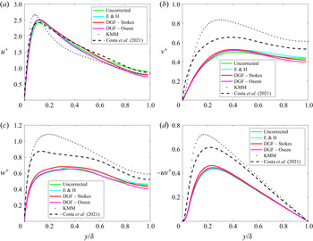
Mean and root-mean-square (r.m.s.) fluid velocity components are shown in figures 10 and 11. For all EL schemes, the mean velocity is enhanced near the centre of the channel, as compared with the particle-free flow, with only modest variation closer to the wall. Similar enhancement was also observed in the simulations of Yamamoto et al. (Reference Yamamoto, Potthoff, Tanaka, Kajishima and Tsuji2001) and Zhao, Andersson & Gillissen (Reference Zhao, Andersson and Gillissen2010). In contrast, the simulations of Costa et al. (Reference Costa, Brandt and Picano2021) show a nominal increase in mean fluid velocity near the channel centre and slight reduction in the mean flow velocity in the overlap region. Costa et al. (Reference Costa, Brandt and Picano2021) remark that their semi-dilute simulation show some signs of a drag-reducing mechanism not seen in their lower mass-loading simulations. They show that increasing mass loading leads to a greater contribution of the momentum balance owing to the particle Reynolds stress and reduction of the fluid Reynolds stress. They suggest that, at high enough mass loading, the fluid Reynolds stress is not sufficient to sustain the turbulence and laminarization leads to drag reduction. We suspect the centreline enhancement of the mean fluid velocity observed in the EL simulations combined with the damping of the wall-normal, spanwise and Reynolds stresses is indicative of the drag-reducing regime to which Costa et al. (Reference Costa, Brandt and Picano2021) alludes. Indeed, the peak intensity drops by nearly a factor of two in each of these components. The streamwise r.m.s. fluid velocity profiles are more complicated with only modest reduction in the peak intensity and a slight enhancement over the bulk of the channel. We observe nominal quantitative variation in predicted fluid statistics for each of the methods over the bulk of the channel. However, the streamwise r.m.s. intensity as predicted by the DGF Oseen method is approximately  $20\,\%$ lower than the trilinear prediction near the channel centre. The DGF Stokes and Esmaily & Horwitz (Reference Esmaily and Horwitz2018) methods also show turbulence reduction at the channel centre. This is perhaps the most significant observation of this study, that accounting for the undisturbed fluid velocity in the particle equation of motion predicts a change in sign of turbulence modification at the channel centre. Previous work in particle-laden isotropic turbulence has shown that accounting for the undisturbed fluid velocity which affects the magnitude of the coupling force can change the magnitude of turbulence modification (Mehrabadi et al. Reference Mehrabadi, Horwitz, Subramaniam and Mani2018; Horwitz & Mani Reference Horwitz and Mani2020), but this is the first study to our knowledge to show that the sign of modification may be affected. It is also worth noting that wall-correcting DGF methods predict lower spanwise and wall-normal r.m.s. components near the channel centre as compared with non-wall-correcting (trilinear and Esmaily & Horwitz Reference Esmaily and Horwitz2018) EL schemes. The observed trends in fluid r.m.s. profiles are in qualitative agreement with the particle-resolved simulations of Costa et al. (Reference Costa, Brandt and Picano2021). In particular, the streamwise r.m.s. profile is in excellent agreement among the simulation methodologies. The wall-normal, spanwise and Reynolds stress profiles show attenuation over the entire channel in the particle-resolved simulations although the magnitude of attenuation is less pronounced than for the EL schemes. We expect the attenuation is higher in these components for the EL schemes because of the higher mass loading of these simulations compared with the particle-resolved case.
Profiles of mean streamwise fluid velocity predicted by different EL schemes in turbulent channel flow. Profiles have been normalized by wall friction velocity of the unladen flow. The black dotted curve shows unladen channel flow data from Kim et al. (Reference Kim, Moin and Moser1987) under similar particle-free conditions. Viscous sublayer and log-layer asymptotes are shown for reference. Also shown are reference particle-resolved data under similar flow conditions (Costa et al. Reference Costa, Brandt and Picano2021).

Profiles of turbulent stresses predicted by different EL schemes in turbulent channel flow. Profiles have been normalized by wall friction velocity of the unladen flow. The black dotted curve shows unladen channel flow data from Kim et al. (Reference Kim, Moin and Moser1987) under similar particle-free conditions. Also shown are reference particle-resolved data under similar flow conditions (Costa et al. Reference Costa, Brandt and Picano2021).

5.2. Particle statistics
Particle concentration profiles for different EL schemes are shown in figure 12. Moving from the wall towards the centre of the channel, the particle concentration profile drops off before recovering nearly linearly and rising to a maximum near the centre of the channel. This qualitative behaviour was observed in the simulation considered by Wang et al. (Reference Wang, Fong, Coletti, Capecelatro and Richter2019) as well as other simulations the authors compared against in that work. The lack of turbophoresis observed can be explained in part owing to the volume fraction considered in this study. Johnson (Reference Johnson2020) showed under a similar turbulence intensity and Stokes number that wall concentration monotonically decreased with increasing volume fraction. The relatively flat concentration profiles were consistent with the relatively flat particle wall-normal velocity profiles (figure 14b). The high wall-normal particle velocity near the wall serves to disperse particles, disrupting turbophoresis, and is consistent with the higher volume fraction considered in this work (Johnson Reference Johnson2020). It is important to note there is a small but noticeable increase in particle concentration inside  $y/\delta < 0.05$. In this region, the dispersive effects of wall-normal fluctuations are counter-acted by wall collisions, which serve to increase accumulation in the wall region. According to Johnson, Bassenne & Moin (Reference Johnson, Bassenne and Moin2020), the qualitative features of the particle concentration profiles can be well approximated in the high Stokes limit as
 $C(y) \sim \mathcal {N}/v_p(y)^2$. Figure 12(b) shows scaled inverse squared particle wall-normal velocity profiles. The inverse wall-normal velocity profiles well capture the qualitative features of the concentration profiles. However, the quantitative differences may be owing to the neglected contribution of biased sampling which is small but non-negligible at the Stokes number considered in this work (Johnson et al. Reference Johnson, Bassenne and Moin2020). Overall, the EL trends compare favourably with the concentration profile of Costa et al. (Reference Costa, Brandt and Picano2021) except very close to the wall where some turbophoresis is evident in the latter simulation. While the EL profiles show slight increase in concentration near the wall, the peak in concentration predicted by the particle-resolved calculation is completely missed by the EL methods. Another difference is that, while the magnitude of the concentration profiles are similar in the bulk, the particle-resolved simulation shows a gentler slope compared with the EL cases. Although we cannot definitively conclude the slopes should be the same owing to slightly different flow conditions, this suggests enhanced importance of biased sampling over turbophoresis in the EL simulations, or in other words, a higher probability of particles experiencing ejection events in the EL simulations compared with the particle-resolved simulation (Johnson et al. Reference Johnson, Bassenne and Moin2020).
Profiles of (a) mean normalized particle concentration and (b) normalized inverse r.m.s. wall-normal particle velocity predicted by different EL schemes in turbulent channel flow. Also shown are reference particle-resolved data under similar flow conditions (Costa et al. Reference Costa, Brandt and Picano2021).

It is also important to note that lift (neglected in this work) can have a dramatic effect on the particle concentration profile even for small particles in dilute regimes (Costa et al. Reference Costa, Brandt and Picano2020). Correcting for wall-damping effects in the particle force model (DGF Stokes and DGF Oseen) resulted in the largest contrast with non-wall-correcting methods for the particle concentration near the channel centre, which was almost  $20\,\%$ higher for the former methods compared with an uncorrected
 $trilinear$ point-particle method. Interestingly, however, these three methods were in good agreement in the prediction of the near-wall particle concentration. The differences in wall/non-wall-correcting EL models and particle-resolved simulation in the predicted concentration profiles were consistent qualitatively with the trends observed in the inverse squared particle wall-normal r.m.s. profiles.
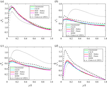
Profiles of mean and r.m.s. particle velocity are shown in figures 13(a) and 14. The overall shape and magnitude of the mean particle velocity near the wall  $U_p/u_{\tau } \approx 6$ agree well with particle-resolved simulations by Horne & Mahesh (Reference Horne and Mahesh2019a,Reference Horne and Maheshb), who studied particle-laden channel flow under similar conditions. The significant enhancement in wall slip velocity was also observed in direct point-particle simulations by Li et al. (Reference Li, Mclaughlin, Kontomaris and Portela2001), point-particle large-eddy simulation (Yamamoto et al. Reference Yamamoto, Potthoff, Tanaka, Kajishima and Tsuji2001) and experiments by Kulick et al. (Reference Kulick, Fessler and Eaton1994) while recent interface resolved simulations (Costa et al. Reference Costa, Brandt and Picano2020) at similar Stokes number but low volume fraction and mass loading show a more modest enhancement in particle velocity at the wall as compared with the mean fluid velocity. Direct comparison of the mean particle velocity of the EL schemes against the semi-dilute case of Costa et al. (Reference Costa, Brandt and Picano2021) shows reasonable agreement near the wall, but the particle-resolved simulation exhibits a slower particle velocity near the channel centre than the EL methods, and this is consistent with the slower mean fluid velocity of the resolved simulation compared with EL simulations. The streamwise, spanwise and wall-normal particle r.m.s. components (figure 14a–c) are in good qualitative agreement with Costa et al. (Reference Costa, Brandt and Picano2021). In addition, the location and magnitude of the peak normal r.m.s. components of the present point-particle simulations are in good agreement with the Costa et al. (Reference Costa, Brandt and Picano2021) simulations, while the peak particle Reynolds stress (figure 14d) observed in the present work is considerably lower than that observed in the interface resolved simulations. This difference, particularly in the particle Reynolds stress, but also to an extent in the particle wall-normal velocity, may be owing to the particle lift force which is especially important in the near-wall region (Costa et al. Reference Costa, Brandt and Picano2020) but which was not considered in the present point-particle simulations.
Profiles of (a) mean streamwise particle velocity normalized by wall friction velocity of the unladen flow and (b) mean particle Reynolds number predicted by different EL schemes in turbulent channel flow. Also shown are reference particle-resolved data under similar flow conditions (Costa et al. Reference Costa, Brandt and Picano2021). Inset shows near-wall profiles of particle Reynolds number.

Profiles of particle r.m.s. components predicted by different EL schemes: (a) streamwise, (b) wall-normal, (c) spanwise and (d) Reynolds stress. Profiles have been normalized by wall friction velocity of the unladen flow. The black dotted curve shows unladen channel flow data from Kim et al. (Reference Kim, Moin and Moser1987) under similar particle-free conditions. Also shown are reference particle-resolved data under similar flow conditions (Costa et al. Reference Costa, Brandt and Picano2021).

The enhancement of particle velocity near the wall can be characterized non-dimensionally as the mean particle Reynolds number  $Re_p = |\bar {U}_f-\bar {U}_p|d_p/\nu$ (figure 13b). To compute this quantity, the mean fluid velocity, which was computed on the non-uniform grid, was interpolated onto a uniform grid which was used to compute an average particle velocity. This may result in some error near the wall. The relatively large particle size
 $d_p^+\approx 2.3$ means that the centre of mass of a particle could never be below the third fluid grid point. To get a reasonable number of particles to average over, the peak in near-wall Reynolds number represents the particle average velocity in a bin around the sixth fluid grid point near
 $y^+\approx 3$. The majority of the channel is characterized by relatively low particle Reynolds number, approximately
 $Re_p \leq 0.5$. In the viscous wall region, the particle Reynolds number is a factor of ten higher, underscoring the importance of inertial effects in the particle drag force as well as in the computation of the undisturbed fluid velocity in the near-wall region. Over the bulk of the channel, the mean particle Reynolds number profiles of the EL simulations are in excellent agreement with the particle-resolved calculation. Near the wall, the particle-resolved calculation predicts a peculiar double peak which is not resolved in the EL simulations. This observation points to missing physics in the EL models such as lubrication effects.
6. Conclusions
We have presented a paradigm for EL two-way coupled simulation involving the method of discrete Green's functions. This method is developed by exploiting linearity of the governing fluid equations. By considering the particular domain and discretization, the disturbance induced by a point source can be recovered exactly. We derived the form of the discrete Green's function for the discrete Stokes equations and calculated the elements of this object for a discrete Stokesian response to a point-force applied at different points and directions between two fixed walls. These curves are the discrete analogues of the continuous analytical solutions obtained by Liron & Mochon (Reference Liron and Mochon1976).
We then considered two verification problems involving the settling of a particle moving parallel to a plane boundary at different wall-normal separations. At low particle Reynolds number, consistent with the employed Stokesian DGF, the discrete Green's function approach performed accurately at all wall-normal separations, compared with existing point-particle schemes which either were accurate in the bulk but not at the wall, or were not accurate at any wall-normal separation. At a particle Reynolds number  $O(1)$, the Stokesian DGF approach remained the most accurate near the wall, but was not as accurate as the Esmaily & Horwitz (Reference Esmaily and Horwitz2018) scheme in the bulk of the channel. Rather than being a limitation of the DGF method, this points to the fact that the Stokesian DGF was being pushed to the edge of its applicability, where self-advection of the disturbance velocity becomes important. To remedy this shortcoming, we have extended the Stokesian DGF methodology to finite particle Reynolds number by appealing to an Oseen-like DGF. The exact form of the Oseen DGF is derived from the discrete Oseen equations. The Oseen DGF components are then related to the Stokesian DGF components with a Reynolds number dependent correlation inspired by Balachandar et al. (Reference Balachandar, Liu and Lakhote2019). The extended DGF methodology is shown to be very accurate in the settling verification problem, showing error in settling velocity less than 6 % at all wall-normal separations tested up to the onset of wake recirculation at
 $Re_p = 24$. (We draw a connection to recent work demonstrating that the method of Green's functions can be used to accurately approximate certain inhomogeneous nonlinear ordinary differential equations (Frasca & Khurshudyan Reference Frasca and Khurshudyan2019). Although requiring more investigation, this suggests adoption of Balachandar et al.'s (Reference Balachandar, Liu and Lakhote2019) correlation to extend the Stokesian DGF or, in other words, the discrete Landau–Squire type solution (Batchelor Reference Batchelor1967) to finite Reynolds number (nonlinear regime) could possibly serve as a basis for extending DGF to other (nonlinear) partial differential equations with source terms.) In a similar fashion, the Esmaily & Horwitz (Reference Esmaily and Horwitz2018) method was pushed to the edge of its applicability in the near-wall region, but recent work (Pakseresht, Esmaily & Apte Reference Pakseresht, Esmaily and Apte2019, Reference Pakseresht, Esmaily and Apte2020) has shown the method of Esmaily & Horwitz (Reference Esmaily and Horwitz2018) can be extended to the wall-bounded regime. Both the Oseen DGF method and extended Esmaily & Horwitz (Reference Esmaily and Horwitz2018) method are comparably accurate point-particle strategies at all wall-normal separations for turbulent channel flow simulation and would likely yield similar predictions over a range of the particle-laden flow parameter phase space.
In the last section, we considered the application of the Stokesian and Oseen DGF methods to the problem of particle-laden turbulent channel flow. On the whole, wall-correcting DGF schemes predicted similar trends in fluid statistics when compared with non-wall-correcting EL schemes. Perhaps the greatest discrepancy observed was in the r.m.s. streamwise fluid velocity, where correcting for the undisturbed fluid velocity consistently showed a reduction in turbulence intensity at the channel centre compared with a completely uncorrected EL scheme. Another important difference observed was in the particle concentration profile near the channel centre. Particle r.m.s. components predicted by the EL schemes also showed their greatest discrepancy near the channel centre. It is perhaps not fortuitous that the particular regime chosen in this study does not highlight a clear quantitative difference among the different EL schemes over the whole channel. On the one hand, it is useful from a modelling standpoint that some of the predicted statistics (at least in certain parts of the flow) are insensitive to fine details of the EL scheme. On the other hand, the necessity of modelling the undisturbed fluid velocity in a wall-bounded environment has been clearly demonstrated. We suspect the highly collisional nature of the present set-up may have belied the importance of properly accounting for wall damping in the particle undisturbed fluid velocity. Understanding the role of wall damping in lower volume fraction regimes where higher turbophoresis is present will be considered in future work. Nevertheless, the comparison against Costa et al.'s (Reference Costa, Brandt and Picano2021) particle-resolved data under similar flow conditions highlights the utility of EL methods to reproduce many of the trends of higher-fidelity calculations.
More work is needed to uncover the discrepancy reported in Segura (Reference Segura2004), who showed that a point-particle large-eddy simulation of turbulent particle-laden channel flow required  $10$ times as many particles as present in the corresponding experiment of Paris (Reference Paris2001) to reproduce the statistics in that data set. Benson, Tanaka & Eaton (Reference Benson, Tanaka and Eaton2005) later determined that wall roughness present in Paris's experiment could explain part of the discrepancy. The observation in this work of significant reduction in streamwise r.m.s. intensity near the channel centre when accounting for the undisturbed fluid velocity suggests that this type of model may have been a missing piece to help explain the observations of Segura (Reference Segura2004). All of these observations continue to point toward heightened attention to numerical details in point-particle simulation as well as direct comparisons (Mehrabadi et al. Reference Mehrabadi, Horwitz, Subramaniam and Mani2018; Costa et al. Reference Costa, Brandt and Picano2020) to elucidate what aspects of numerical simulations are indeed physical and which ones still require more careful modelling in order to reproduce higher-fidelity particle-resolved simulations and experiments. In particular, it appears that neglecting the particle lift force is justified for some but not all particle statistics.
The extension of the DGF method to finite Reynolds number makes it an attractive approach compared with the extended ERPP approach, which is based on analytical solutions to the unsteady Stokes equations (Battista et al. Reference Battista, Mollicone, Gualtieri, Messina and Casciola2019). However, the ERPP approach may be more advantageous in regimes where the density ratio is not exceptionally large, such as liquid–solid flow. There, unsteady drag, e.g. history and added-mass effects, is important and an ERPP-type analytical solution in this case could be more favourable in comparison with storing time-dependent DGFs. Another potential advantage that DGF offers is the ability to estimate undisturbed quantities for PDEs and/or domains where analytical Green's functions owing to regularized point-source terms are unknown or cumbersome to express in closed form. (Compare the Green's function of Blake & Chwang (Reference Blake and Chwang1974) with that of Liron & Mochon (Reference Liron and Mochon1976) which should be similarly reliable for a small particle near a single plane wall but the latter work which accounts for the presence of a second wall is expressed in a comparatively complicated form.) Finally, the extension to finite particle Reynolds numbers distinguishes the present work from other types of simulation methodologies which are highly accurate for Stokesian particle-laden flows including Stokesian dynamics (Swan & Brady Reference Swan and Brady2010), force coupling (Maxey Reference Maxey2017), and regularized Stokeslets (Cortez Reference Cortez2001).
This work, besides providing a practical approach to estimate undisturbed quantities in EL simulation, provides insight into the intimate connection among interpolation/projection stencil (for example, Lagrange polynomial vs Gaussian) for EL transfer, governing fluid equations and their numerical discretization (second- vs fourth-order finite difference)/element structure (structured vs unstructured) and boundary conditions (periodic vs wall) and the ultimate discrete response generated by discrete source terms. While we have applied this method to hydrodynamic equations, we expect this approach would be of value in the consideration of thermal and electricity/magnetism effects experienced by particles. The DGF formulation presented here is reminiscent of the mobility function concept (Kim & Karrila Reference Kim and Karrila2005), and by analogy could be extended to torque coupling as well. The Stokesian DGFs obtained for this work may be of value to other researchers conducting investigations of particle-laden channel flow and we can make these DGFs available upon request.
Acknowledgements
We benefited from discussions with P. Johnson and with M. Esmaily, whose code was used to perform the simulations presented in the present work. We are grateful to P. Costa, L. Brandt and F. Picano for sharing their particle-resolved data to support a comparison with the present simulations. We would also like to thank the anonymous reviewers for their constructive feedback.
Funding
Funding was provided through a US Department of Energy grant for the Predictive Science Academic Alliance Program 2 (PSAAP2) at Stanford University under grant number DE-NA0002373. This work was performed under the auspices of the US Department of Energy by Lawrence Livermore National Laboratory under contract DE-AC52-07NA27344, LLNL-JRNL-818319.
Declaration of interests
The authors report no conflict of interest.
Appendix A. Extension of discrete Green's functions to finite Reynolds number
Here, we consider a finite Reynolds number extension to the Stokes discrete Green's function. The base fluid flow is  $\boldsymbol {\bar {u}}=(\bar {U}(y),0,0)$, and we denote the perturbation induced by the two-way coupling force as
 $\boldsymbol {u'}$. Starting with the steady Navier–Stokes equation and writing the fluid velocity as
 $\boldsymbol {u}= \boldsymbol {\bar {u}}+\boldsymbol {u'}$, we have
 $$\begin{gather} \rho_f u_j\frac{\partial u_i}{\partial x_j}=\mu\frac{\partial^2 u_i}{\partial x_j\partial x_j}-\frac{\partial p}{\partial x_i}- F_{i}, \end{gather}$$
 $$\begin{gather}\frac{\partial^2 p}{\partial x_j\partial x_j} ={-}\rho_f \frac{\partial u_j}{\partial x_i}\frac{\partial u_i}{\partial x_j} -\frac{\partial F_i}{\partial x_i}. \end{gather}$$
The advection term,  $u_j({\partial u_i}/{\partial x_j})$ can be decomposed as
 \begin{equation} u_j\frac{\partial u_i}{\partial x_j}=\bar{u}_j\frac{\partial \bar{u}_i}{\partial x_j}+\bar{u}_j\frac{\partial u'_i}{\partial x_j}+u'_j\frac{\partial \bar{u}_i}{\partial x_j}+u'_j\frac{\partial u'_i}{\partial x_j}. \end{equation}
The first term in (A3) is identically zero. The remaining terms can be written, along with their associated scalings, as (the proper scaling near the wall,  $\sim {u'\bar {U}}/{\mathrm{\Delta} }$ is hereby noted, and the current analysis can be analogously extended to include this term)
 $$\begin{gather} \bar{u}_j\frac{\partial u'_i}{\partial x_j} = \bar{U}\left(\frac{\partial u'}{\partial x},\frac{\partial v'}{\partial x},\frac{\partial w'}{\partial x}\right)\sim \frac{u'\bar{U}}{\mathrm{\Delta}}, \end{gather}$$
 $$\begin{gather}u'_j\frac{\partial \bar{u}_i}{\partial x_j}=\left(v'\frac{\partial \bar{u}}{\partial y},0,0\right)\sim \frac{u'\bar{U}}{\delta}, \end{gather}$$
 $$\begin{gather}u'_j\frac{\partial u'_i}{\partial x_j} \sim \frac{u'^2}{\mathrm{\Delta}}. \end{gather}$$
Using typical channel dimensions, grid spacing and disturbance velocity scalings,
 \begin{equation} \bar{u}_j\frac{\partial u'_i}{\partial x_j}\gg \left\{u'_j\frac{\partial \bar{u}_i}{\partial x_j}, u'_j\frac{\partial u'_i}{\partial x_j} \right\}. \end{equation}
Therefore, we seek the discrete Green's function associated with the reduced discrete linearized Oseen system
 $$\begin{gather} \rho_f \bar{u}^n_j\frac{\delta u^n_i}{\delta x_j} = \mu\frac{\delta^2u_i^n}{\delta x_j \delta x_j}-\frac{\delta p^n}{\delta x_i}- F_{i}^n, \end{gather}$$
 $$\begin{gather}\frac{\delta^2 p^n}{\delta x_j \delta x_j} ={-}\rho_f \frac{\delta \bar{u}^n_j}{\delta x_i}\frac{\delta u^n_i}{\delta x_j} -\frac{\delta F_i^n}{\delta x_i}. \end{gather}$$
Defining the following discrete differential operators:  $C^{kn} \equiv (\nabla ^2)^{-1}$,
 $A_j()_j\equiv ({\partial }/{\partial x_j})()_j$ and
 $B_{i} =\boldsymbol {\nabla }$, and the quantity,
 $D^{n}_i = \rho _f\bar {u}_j^n B_j u_i^n$ with no summation of the upper indices, we can write the formal solution to (A8) and (A9) as (the (
 $p$) superscript is used to emphasize that while the velocity is evaluated at grid point
 $p$, there is no summation of index
 $p$)
 $$\begin{gather} p^k ={-}C^{kn}\{\ A_i D^{n}_i + A_jF_j^n \}, \end{gather}$$
 $$\begin{gather}\{\delta^{kp}_{ij}- B_iC^{kp} A_j\} D^{p}_j - \mu A_jB_ju_i^k = \{ B_iC^{kp} A_j - \delta_{ij}^{kp}\}F_j^p, \end{gather}$$
 $$\begin{gather}\{\delta^{kp}_{ij}- B_iC^{kp} A_j\} \rho_f\bar{u}_m^{(p)} B_m u_j^p - \mu A_jB_ju_i^k = \{ B_iC^{kp} A_j - \delta_{ij}^{kp}\}F_j^p, \end{gather}$$
 $$\begin{gather}\{\delta^{kp}_{ij}- B_iC^{kp} A_j\} \rho_f\bar{u}_m^{(p)} B_m u_j^p - \mu A_mB_m\delta_{ij}^{kp} u_j^p = \{ B_iC^{kp} A_j - \delta_{ij}^{kp}\}F_j^p, \end{gather}$$
 $$\begin{gather}\{ \{\delta^{kp}_{ij}- B_iC^{kp} A_j\} \rho_f\bar{u}_m^{(p)} B_m - \mu A_mB_m\delta_{ij}^{kp} \}u_j^p = \{B_iC^{kp} A_j - \delta_{ij}^{kp}\}F_j^p. \end{gather}$$
By letting  $E^{nk} = \{ \{\delta ^{kp}_{ij}- B_iC^{kp} A_j\} \rho _f\bar {u}_m^{(p)} B_m - \mu A_mB_m\delta _{ij}^{kp} \}^{-1}$ and
 $G_{ij}^{np} = E^{nk}\{B_iC^{kp} A_j - \delta _{ij}^{kp}\})$, (A14) can be written in a simpler form
 \begin{equation} u_i^n = G_{ij}^{np}F_j^p. \end{equation}
Appendix B. Relationship between Oseen and Stokes discrete Green's functions
The new Oseen DGF can be related to the Stokes DGF,  $G_{ij}^{np} = \mu ^{-1}C^{nk}(\delta _{ij}^{kp}-B_iC^{kp}A_j)$, found previously.
Performing algebra on the Oseen DGF, we have
 $$\begin{gather} G_{ij}^{np} =\{ \{\delta^{kp}_{ij}- B_iC^{kp} A_j\} \rho_f\bar{u}_m^{(p)} B_m - \mu A_mB_m\delta_{ij}^{kp} \}^{{-}1}\{B_iC^{kp} A_j - \delta_{ij}^{kp}\}, \end{gather}$$
 $$\begin{gather}G_{ij}^{np} =\{\mu A_mB_m\delta_{ij}^{kp} - \{ \delta^{kp}_{ij}- B_iC^{kp} A_j\} \rho_f\bar{u}_m^{(p)} B_m \}^{{-}1}\{ \delta_{ij}^{kp} - B_iC^{kp} A_j\}, \end{gather}$$
 $$\begin{gather}G_{ij}^{np} =\{ A_mB_m\delta_{ij}^{kp} - \{ \delta^{kp}_{ij}- B_iC^{kp} A_j\} \mu^{{-}1}\rho_f\bar{u}_m^{(p)} B_m \}^{{-}1} \mu^{{-}1} \{ \delta_{ij}^{kp} - B_iC^{kp} A_j\}, \end{gather}$$
 $$\begin{gather}G_{ij}^{np} =\{ (C^{nk})^{{-}1}\delta_{ij}^{kp} - \{ \delta^{kp}_{ij}- B_iC^{kp} A_j\} \mu^{{-}1}\rho_f\bar{u}_m^{(p)} B_m \}^{{-}1} \mu^{{-}1} \{ \delta_{ij}^{kp} - B_iC^{kp} A_j\}. \end{gather}$$
Using the Woodbury inversion formula  $(A+UCV)^{-1} = A^{-1}-A^{-1}U(C^{-1}+V A^{-1} U)^{-1} V A^{-1}$, with
 $A = (C^{nk})^{-1}\delta _{ij}^{kp}$,
 $U = - \{ \delta ^{kp}_{ij}- B_iC^{kp} A_j\}$,
 $C = \mu ^{-1}\rho _f$, and
 $V = \bar {u}_m^{(p)} B_m$, we have
 \begin{align} &\{ (C^{nk})^{{-}1}\delta_{ij}^{kp} - \{ \delta^{kp}_{ij}- B_iC^{kp} A_j\} \mu^{{-}1}\rho_f\bar{u}_m^{(p)} B_m \}^{{-}1} \nonumber\\ &\quad =((C^{nk})^{{-}1}\delta_{ij}^{kp})^{{-}1}+((C^{nk})^{{-}1}\delta_{ij}^{kp})^{{-}1} (\{ \delta^{kp}_{ij}- B_iC^{kp} A_j\})((\mu^{{-}1}\rho_f)^{{-}1}\nonumber\\ &\qquad +(\bar{u}_m^{(p)} B_m) ((C^{nk})^{{-}1}\delta_{ij}^{kp})^{{-}1} (- \{ \delta^{kp}_{ij}- B_iC^{kp} A_j\}))^{{-}1} (\bar{u}_m^{(p)} B_m) ((C^{nk})^{{-}1}\delta_{ij}^{kp})^{{-}1}. \end{align}
Using  $((C^{nk})^{-1}\delta _{ij}^{kp})^{-1} = (\delta _{ij}^{kp})^{-1}(C^{nk}) = \delta _{ij}^{kp}C^{nk}$,
 \begin{align} &\{ (C^{nk})^{{-}1}\delta_{ij}^{kp} - \{ \delta^{kp}_{ij}- B_iC^{kp} A_j\} \mu^{{-}1}\rho_f\bar{u}_m^{(p)} B_m \}^{{-}1} \nonumber\\ &\quad =\delta_{ij}^{kp}C^{nk}+\delta_{ij}^{kp}C^{nk}( \{ \delta^{kp}_{ij}- B_iC^{kp} A_j\})((\mu^{{-}1}\rho_f)^{{-}1}\nonumber\\ &\qquad-(\bar{u}_m^{(p)} B_m) \delta_{ij}^{kp}C^{nk} (\{ \delta^{kp}_{ij}+ B_iC^{kp} A_j\}))^{{-}1} (\bar{u}_m^{(p)} B_m) \delta_{ij}^{kp}C^{nk}\nonumber\\ &\quad =\{\delta_{ij}^{kp}+\delta_{ij}^{kp}C^{nk}( \{ \delta^{kp}_{ij}- B_iC^{kp} A_j\})((\mu^{{-}1}\rho_f)^{{-}1}\nonumber\\ &\qquad-(\bar{u}_m^{(p)} B_m) \delta_{ij}^{kp}C^{nk} (\{ \delta^{kp}_{ij}+ B_iC^{kp} A_j\}))^{{-}1} (\bar{u}_m^{(p)} B_m) \delta_{ij}^{kp}\} C^{nk}. \end{align}
The terms contained within the braces can now be recognized as the deviation from the Stokesian DGF.
With a little more algebra it can be seen that
 \begin{align} &\{ (C^{nk})^{{-}1}\delta_{ij}^{kp} - \{ \delta^{kp}_{ij}- B_iC^{kp} A_j\} \mu^{{-}1}\rho_f\bar{u}_m^{(p)} B_m \}^{{-}1} \nonumber\\ &\quad =\{\delta_{ij}^{kp}+\delta_{ij}^{kp}C^{nk}( \{ \delta^{kp}_{ij}- B_iC^{kp} A_j\})(1-(\rho_f/\mu) (\bar{u}_m^{(p)} B_m) \delta_{ij}^{kp}C^{nk} (\{ \delta^{kp}_{ij} \nonumber\\ &\qquad + B_iC^{kp} A_j\}))^{{-}1} (\rho_f/\mu)(\bar{u}_m^{(p)} B_m) \delta_{ij}^{kp}\} C^{nk}. \end{align}
In a more compact form, this allows the Oseen and Stokes discrete Green's functions to be related by the following expression:
 \begin{equation} \boldsymbol{G}^{Oseen}=f(\boldsymbol{Re})\boldsymbol{G}^{Stokes}, \end{equation}
where  $\boldsymbol {Re}=(\rho _f/\mu )C^{nk}(\bar {u}_m^{(p)} B_m) \delta _{ij}^{kp}$ is a Reynolds tensor which scales with the local mesh Reynolds number.
Appendix C. Closure of Oseen DGF coefficients and verification at finite Reynolds numbers
The expression relating the Stokes and Oseen discrete Green's function is very complicated and does not provide a simple closed form expression for the Oseen DGF components. Practically, numerical values of the Oseen DGF components could be derived using the same procedure as for the Stokesian DGF components in § 3. However, this procedure would have to be repeated for different Reynolds numbers and establishing Reynolds number bounds on the coefficients would be cumbersome. To circumvent these issues, we appeal to the correlation developed by Balachandar et al. (Reference Balachandar, Liu and Lakhote2019). In that work, an analytical solution to the Oseen equations was developed subject to a Gaussian force density in an unbounded domain. By performing simulations of this point-force density at different non-dimensional force strengths and Reynolds numbers, they extended the analytical solution for the magnitude of the velocity response at a particle location outside the low Reynolds number range. In the language of the present work, they developed a finite Reynolds number DGF assuming the DGF tensor is isotropic. We adopt their correlation here to close the function  $f(\boldsymbol {Re})$ in (B8). In particular, this function takes the form (using the notation in) Balachandar et al. (Reference Balachandar, Liu and Lakhote2019)
 \begin{equation} f(\boldsymbol{Re})=\varPsi_{Os}(Re_{\sigma})\chi(Re_{\sigma},|\tilde{F}|), \end{equation}
where
 $$\begin{gather} \varPsi_{Os}(Re_{\sigma}) = \frac{3}{\sqrt{2{\rm \pi}}}\frac{{\rm \pi}-\sqrt{2{\rm \pi}}Re_{\sigma}+({\rm \pi}/2)Re_{\sigma}^2-{\rm \pi} \exp(Re_{\sigma}^2/2)erfc(Re_{\sigma}/\sqrt{2})}{Re_{\sigma}^{3}}, \end{gather}$$
 $$\begin{gather}\chi(Re_{\sigma},|\tilde{F}|) = 10^{A(Re_{\sigma})|\tilde{F}|+B(Re_{\sigma})|\tilde{F}|^{2}}. \end{gather}$$
In the previous expressions,  $Re_{\sigma }$ is the Reynolds number based on the standard deviation of the Gaussian used as the point-force mollifier in Balachandar et al. (Reference Balachandar, Liu and Lakhote2019),
 $|\tilde {F}| = 3{\rm \pi} (1+0.15Re_{p}^{0.687})/Re_{p}({d_p}/{\sigma })^{2}$ is the non-dimensional force magnitude consistent with the Schiller–Naumann drag adopted in this work,
 $A(Re_{\sigma })=0.118\exp (-3.16Re_{\sigma }^{-0.88})$ and
 $B(Re_{\sigma })=0.084\exp (-5.54Re_{\sigma }^{-0.76})$. The resulting expressing for
 $f(\boldsymbol {Re})$ approaches unity at small Reynolds number consistent with the Oseen DGF components recovering the Stokesian DGF components in this limit.
Two caveats are worth noting. First, while the present DGF methodology is consistent with Gaussian projection schemes, we have used a trilinear projection scheme so that a different definition of  $\sigma$ is needed. Here, we take the relevant length scale to be the cube root of the cell volume
 $\sigma \approx (\textrm {d}\kern0.7pt x\, \textrm {d} y\, \textrm {d} z)^{1/3}$. Second, the correlation proposed by Balachandar et al. (Reference Balachandar, Liu and Lakhote2019) is for an unbounded flow yet our work has been concerned primarily with a wall-bounded configuration. We suggest and confirm fortuitously that, since the Stokesian DGF components we have derived in this work already build in wall-damping effects, the anisotropy needed is to determine how the magnitude of the velocity response changes at the location of the application of the point force, as the disturbance advects downstream with increasing Reynolds number (see figure 2 in the referenced work). This is the scaling adopted in (C1).
To test the appropriateness of the Balachandar correlation for the Oseen DGF components, we show results for the verification exercise discussed in § 4 of a particle settling under gravity at different Reynolds numbers parallel to a wall (figure 15). Up to a particle Reynolds number of 24, the Oseen DGF methodology allows the prediction of the particle settling velocity with an error less than 6 % at all wall-normal separations tested. This upper bound was chosen since it represents the onset of recirculation in the wake of a sphere (Taneda Reference Taneda1956). This recirculation is the simplest flow structure that cannot at present be represented in any form by an EL scheme. Below this critical Reynolds number, the disturbance flow especially at large distances is well approximated by the numerically regularized Landau–Squire jet, which is in fact a solution of the point-particle equations (Batchelor Reference Batchelor1967; Horwitz & Mani Reference Horwitz and Mani2018). The onset of vortex recirculation also represents particle-induced disturbance flow which may couple to the background turbulence (Bagchi & Balachandar Reference Bagchi and Balachandar2004). Although the present Oseen-extended DGF methodology may be accurate in computing the motion of a single sphere at higher Reynolds number in the verification sense, we have chosen not to present that demonstration in an effort to reduce the chance a modeller adopts the present approach in a regime where these types of more complicated physical couplings are critical to the understanding of those applications. Alternatively, there may be applications where EL predictions incorporating mean particle drag are fully suitable to characterize engineering quantities within reasonable tolerance even if the methodology itself is not able to capture the vortex shedding of individual spheres. Nevertheless, the results of this section provide confidence that the extended DGF methodology is accurate for the simulation of practical engineering flows such as particle-laden channel flows.
Percentage error in settling velocity predicted by the Oseen DGF method for a two-way coupled particle moving parallel to a plane wall for different wall-normal separations and particle Reynolds numbers.

Appendix D. Staggered grid considerations
The staggered grid incorporated in this work, shown in figure 16, in general requires more storage per wall-normal location than the  $24\times 24$ elements required for a collocated configuration. To illustrate this, consider a particle travelling exclusively in the streamwise direction from the
 $x$-coordinate of
 $w_{17}$ to the
 $x$-coordinate of
 $w_{18}$. The initial y-coordinate is the same as that of
 $u_{1}$ and the initial z-coordinate is half-way between the z-coordinate of
 $u_{1}$ and
 $u_{3}$. When the particle passes the x-coordinate of
 $u_{2}$, interpolation and projection of Lagrangian information will now require information from
 $u$-cell faces downstream, outside of the set
 $u_{1-8}$, even though the grid points associated with spanwise and wall-normal interpolations remain unchanged. In other words, figure 16 depicts one of eight needed interpolation stencils for a trilinear configuration. This presents no issue for the diagonal blocks of the DGF elements since, for example the
 $G^{25,25} = G^{1,1}$, where
 $25$ is the downstream streamwise cell face considered in the previous example. Similarly
 $G^{1,2}=G^{2,25}$ etc. However, the issue is that the element
 $G^{21,25}$, for example, in other words an off-diagonal block element is not equal to any of the
 $24\times 24$ stored elements. In general, this means a staggered grid implementation of DGF requires more elements than the collocated grid counterpart. To reduce storage cost, however, we have chosen to store the DGF elements associated with the canonical arrangement shown in figure 16. This means that when using (2.8) to estimate the undisturbed fluid velocity vector,
 $W^{k}$ and
 $w^{n}$ will provide the correct interpolation weights but certain off-diagonal block elements of the DGF matrix outside the canonical configuration will be approximated based on DGF elements obtained in the canonical configuration. This approximation will lead to negligible error because off-diagonal blocks constitute a small correction to that contributed by diagonal blocks of the DGF matrix. In other words, for a three-dimensional force, most of the x-component of the response, for example, is contributed by the x-component of the force projected to streamwise cell faces. This is readily apparent in figure 5. The elements of the diagonal blocks are clearly much greater than the elements of the off-diagonal blocks. The exception is the wall-normal block near the wall (figure 5a), because a wall-normal response cannot be generated close to the wall. To quantify the importance of the diagonal blocks, the square of the Frobenius norm of the whole DGF matrix is compared with the sum of the squares of the Frobenius norms of the diagonal blocks, that is
 $(|G^{(1:8,1:8)}|^{2}+|G^{(9:16,9:16)}|^{2}+|G^{(17:24,17:24)}|^{2})/|G^{(1:24,1:24)}|^{2}$. The respective ratios for the near-wall and near-centre DGF matrices are approximately
 $0.97$ and
 $0.95$, thus demonstrating dominance of the diagonal block elements. The success of the present implementation of a Stokesian DGF is corroborated by the low Reynolds number verification study shown in § 4.1.
Grid points involved in trilinear interpolation and projection for the staggered arrangement considered in this work. For an arbitrary location of a particle in the domain, the surrounding grid points can be mapped to the notation used here. Streamwise cell faces are denoted with  $u$, spanwise with
 $w$ and wall normal with
 $v$.