1. Introduction
Following the seminal work of Sachs and Warner (Reference Sachs and Warner1995), a huge literature has developed on the so-called resource curse. The latter refers to the paradox that resource-abundant countries experience lower long-run economic growth than do resource-poor countries. A number of transmission channels have been put forward in the literature to explain this curse. These channels can be split up into two categories: economic mechanisms and political explanations.
Among the economic transmission channels, the most popular is the ‘Dutch disease’, which has been widely documented in the literature (see for example Bruno and Sachs, Reference Bruno and Sachs1982; Corden, Reference Corden1984; Krugman, Reference Krugman1987; Torvik, Reference Torvik2001; Matsen and Torvik, Reference Matsen and Torvik2005). This refers to the over-evaluation of the local currency following the discovery and exploitation of a significant new resource deposit. This currency appreciation causes a loss of competitiveness in the secondary and tertiary sectors that are the engines of growth (increasing returns to scale and positive externalities are more likely to be found in the secondary and tertiary sectors than in the primary sector). Alongside the Dutch disease, we can note that mining is largely an enclave industry. As such, the extraction of mineral resources per se will produce relatively few positive spillovers for the rest of the economy (Davis and Tilton, Reference Davis and Tilton2005; Humphreys et al., Reference Humphreys, Sachs and Stiglitz2007). Abundant natural resources may also crowd out human-capital investment, increasing agents’ opportunity costs of investing in human capital (Sachs and Warner, Reference Sachs and Warner1999; Gylfason, Reference Gylfason2001). In addition, natural resource discoveries shift investment from the secondary and tertiary sectors to the extractive industry, which is less likely to generate productivity gains (Sachs and Warner, Reference Sachs and Warner1995). The other main economic channels include resource-price volatility. The main source of revenues in resource-rich countries is often the extractive sector. However, resource prices can vary substantially, affecting the ability of governments to successfully manage their rent. The macroeconomic instability that results from resource-price volatility can also discourage investment (Daniel, Reference Daniel and Tilton1992; van der Ploeg and Poelhekke, Reference van der Ploeg and Poelhekke2009, Reference van der Ploeg and Poelhekke2010).
There also exist various political transmission channels. Natural resources first generate rents, which may be misused. Resource rents allow governments to avoid or postpone unpopular but necessary structural reforms, and may also be devoted to unproductive welfare expenditures (Bomsel, Reference Bomsel and Tilton1992). Ross (Reference Ross1999) also notes that nationalized mining companies may soften the budget constraint of resource-exporting governments, ‘producing fiscal laxity and a tendency to over-borrow’. In addition, natural resources may encourage weak institutions: resource-rich countries are often characterized by centralized power and collusion between public authorities and the mining industry. Moreover, resource revenues may be used in order to mollify dissent, repress opposition and avoid accountability pressure (Karl, Reference Karl1999). With weak institutions, natural resources incite rent-seeking behaviors by political interest groups. Those groups often ask for transfers that do not reflect economic contributions or social value. Corruption is also a major concern in resource-rich economies: politicians are often suspected of embezzling rents for their own personal gain or accepting bribes from third parties who wish to obtain or conserve access to the rent. Last, natural resources can generate conflicts for greed or grievance motives. Under the greed theory, rebels begin armed conflict in order to obtain access to or secure resource revenues. The grievance theory on the contrary suggests that rebels are motivated by the rising inequality that follows a resource boom (caused by rent-seeking, corruption and so on). In this latter case, social justice is the main source of conflict. There are obviously many causes of war, among which appear natural resources. These have been shown to often cause longer conflicts by providing the belligerents with revenues.
Alongside this transmission-channel literature, there has been great debate over the evidence for the existence of the resource curse. Lederman and Maloney (Reference Lederman and Maloney2006, Reference Lederman and Maloney2008) carefully discuss the evidence in the literature and explain that it is difficult to talk about a curse. They review the literature on each channel and argue that for some channels the curse is not convincingly present. For other channels, they claim that the curse is not very specific to resources. Indeed, there exists evidence that there is no curse in the strictest sense of the word, because the underlying mechanisms also apply for non-resource goods. For example, the negative effects that natural resources may have on institutional quality described earlier (through rent seeking, conflicts, etc.) are not specific to natural resources but concern any sources of rents. When the channel is not convincingly demonstrated, this is often because the results found by Sachs and Warner (Reference Sachs and Warner1995) and other authors using the share of resource exports in GDP as a proxy for resource abundance are not robust to the use of other resource-abundance indicators and different econometric methodologies.
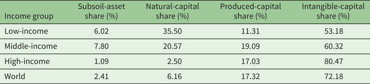
In this spirit, Stijns (Reference Stijns2006) shows that the crowding-out effect of resource abundance on human capital disappears when resource wealth is measured with more appropriate metrics.Footnote 1 This ambivalence in the literature is driven by the empirical observation that resource-rich countries have diverse experiences. First of all, natural resources have historically been the engine of growth of developed countries. Indeed, the use of mineral resources was the very source of the two first industrial revolutions, and the success story of the United-States since independence represents one of the best illustrations. However, it seems that this positive relationship between resource endowments and economic development has reversed since the 1960s. For example, as Nigeria's oil revenues rose sharply between 1966 and 2010, its real GDP per capita in constant PPP was multiplied by a factor of 2.2.Footnote 2 Equally, Botswana was one of the poorest countries in the world when it gained independence in 1966, but has enjoyed one of the highest growth rates over the past four decades, thanks to its diamond deposits. Its GDP per capita in constant PPP rose by a factor of 14.8 over this periodFootnote 3 : it is now one of the richest African countries and left the least-developed economies group in 1994.Footnote 4 Indonesia, Malaysia, and Thailand have also often been cited (together with Botswana) as developing, resource-rich economies that have achieved a long-term investment ratio of over one-quarter of GDP. While some suggest that these countries have escaped the resource curse, they still appear to have performed less well than their neighbors who have fewer raw materials: Hong Kong, Singapore and South Korea (van der Ploeg, Reference van der Ploeg2011).Footnote 5 The World Bank estimates in table 1 show that subsoil-asset and natural-capital shares are higher in low- and middle-income economies than in developed countries. Symmetrically, the intangible-capital share rises with the level of development.
Total wealth and subcomponents in 2005

These are per capita figures. Source: Own calculations based on Lange et al. (Reference Lange, Hamilton, Ruta, Chakraborti, Desai, Edens, Ferreira, Fraumeni, Jarvis, Kingsmill and Li2010).
Growth regressions are often used to investigate the resource curse. The growth regressions in the seminal paper by Sachs and Warner (Reference Sachs and Warner1995) show that the natural-resource share of exports is negatively correlated with economic development. They then extend their work to show that there is little evidence that the curse is explained by omitted geographical variables (Sachs and Warner, Reference Sachs and Warner2001). Atkinson and Hamilton (Reference Atkinson and Hamilton2003) use growth regressions to suggest that the resource curse reflects the inability of governments to manage large resource revenues in a sustainable way. Papyrakis and Gerlagh (Reference Papyrakis and Gerlagh2004) also use growth regressions to analyze resource-curse transmission channels. Alongside these positive analyses, some normative work also relies on growth regressions. Among others, Sala-i-Martin and Subramanian (Reference Sala-i Martin, Subramanian, Collier, Soludo and Pattillo2008) suggest that resource-rich economies (and, more precisely, Nigeria) should directly distribute their oil revenues to the population.
The empirical evidence for a curse that uses growth regressions is a source of controversy. The most skeptical paper on those findings is perhaps the one by Brunnschweiler and Bulte (Reference Brunnschweiler and Bulte2008), who argue that the use of growth regressions in this literature is often accompanied by two sizeable problems: (i) natural-resource exports over GDP capture resource dependence rather than resource abundance, and their use as a proxy for abundance may lead to the misinterpretation of the regression results; and (ii) introducing resource dependence and institutional variables in growth regressions may lead to endogeneity bias, as resource dependence is related to economic choices that may simultaneously affect growth. Natural resources can also reduce institutional quality, which in turn affects resource dependence through the economic policies that depend on institutions. The authors address this endogeneity problem via Three-Stage Least Squares (3SLS) regressions using historical openness and having a Presidential regime in the 1970s as instruments for resource dependence, while institutional quality is instrumented by latitude.Footnote 6 They conclude that resource abundance has a positive effect on economic growth, while resource dependence has no effect: the resource curse may then be a red herring.
Brunnschweiler and Bulte (Reference Brunnschweiler and Bulte2008) introduce regional dummies to pick up the differences in average economic growth across regions, conditional on the other explanatory variables. However, this choice of regions needs to be discussed and justified, as countries in the same region do exhibit considerable heterogeneity in terms of climate, geology, culture, politics and economics. Using the same dataset, Clootens and Kirat (Reference Clootens and Kirat2017) show that the impact of resource dependence on growth becomes strongly negative and significant when the regional dummies are omitted. Moreover, the way in which Brunnschweiler and Bulte (Reference Brunnschweiler and Bulte2008) take regional heterogeneity into account constrains the model parameters (apart from the constant) to be identical across regions. Durlauf and Johnson (Reference Durlauf and Johnson1995) show that the linear model that is commonly used to analyze growth behavior may be misspecified, and argue for a multiple-regime alternative.
Clootens and Kirat (Reference Clootens and Kirat2017) relax this linearity assumption and allow all estimated parameters to vary by region. They split the sample into two distinct regions: the Northern and Southern countries.Footnote 7 As this split is subjective, they also look at OECD versus non-OECD countries. They find that Southern (non-OECD) and Northern (OECD) economies have different relations to resource dependence: resource dependence reduces growth in low-income economies.
The sample split in Clootens and Kirat (Reference Clootens and Kirat2017) is subjective, and could be improved by the use of formal sample-splitting methods. Konte (Reference Konte2013) argues that the impact of natural resources on growth may depend on the growth regime to which the country belongs. Using regression-mixture methods, she shows that natural resources increase growth in some countries but reduce it in others.
We use here the sample-splitting approach in Hansen (Reference Hansen2000) to test for a threshold effect, and estimate the threshold endogenously rather than arbitrarily selecting the value. This approach is motivated by the fact that the relationships between growth and its determinants are non-linear. Indeed, it is well-known from the literature on growth that countries experience various growth regimes. This idea was first developed by Durlauf and Johnson (Reference Durlauf and Johnson1995), who suggest that cross-section growth may be determined by initial conditions. Hansen (Reference Hansen2000) extends the work by Durlauf and Johnson (Reference Durlauf and Johnson1995) and uses initial GDP and literacy as threshold variables in growth regression to distinguish multiple equilibria. This is why we go further and extend this latter idea to assess whether the impacts of resource abundance and resource dependence on growth are regime-dependent. We believe that this approach has notable advantages, as it allows us to correct for potential endogeneity bias provided that our splitting variable is exogenous. Indeed, Caner and Hansen (Reference Caner and Hansen2004) show that this method allows the use of instrumental variables instead of ordinary least squares to address the potential endogeneity of right-hand-side variables. This method requires the exogeneity of the threshold variable. In our application, initial GDP seems exogenous because initial period characteristics suffer less from reverse causality concerns. We estimate the threshold value of initial GDP that allows the sample to be split in two. Then we run regressions on our sub-samples. We find that resource dependence reduces growth in low-income economies, while resource abundance is on the contrary a blessing. Growth in high-income countries is not significantly affected by either abundance or dependence.
The remainder of the paper is organized as follows. Section 2 describes the data and section 3 sets out the estimation strategy. Section 4 then presents the results and their interpretation. Last, section 5 concludes.
2. Data
One of the main purposes of this paper is to explain the differences in long-run growth between countries. To this end, our econometric analysis below is carried out on a cross-sectional dataset of 83 countries covering the period 1980--2014. This section describes all of the variables used in our analysis and clarifies the differences among the most commonly-used indicators in the literature to measure resource abundance and resource dependence. Section 2.1 introduces our dependent variable while section 2.2 discusses in detail the explanatory variables. Section 2.3 deals with the instrumental variables.
2.1. The dependent variable
The variable ${\rm Growth}$ is the dependent variable. This variable refers to the average log-growth of real (PPP in constant dollars) GDP per capita between 1980 and 2014. The Penn World Table 9.0 provides five GDP estimates: here we use real GDP calculated using national accounts growth rates, as recommended for growth regressions by Feenstra et al. (Reference Feenstra, Inklaar and Timmer2015).Footnote 8
2.2. The explanatory variables
This paper tries to disentangle resource-abundance effects from resource-dependence ones, in a way that follows Brunnschweiler and Bulte (Reference Brunnschweiler and Bulte2008). In all our regressions, we consequently include a resource-abundance variable together with a resource-dependence variable as regressors. In addition, we include different variables capturing the institutional quality, the level of investment, human capital and population growth, as well as the initial GDP. All of these explanatory variable are described hereafter.
We use alternatively two indicators of resource abundance (RA). ${\rm RA}_{1}$ is the log of the World Bank subsoil asset natural capital per capita indicator averaged over the period. Natural capital includes the valuation of numerous minerals and fuels. This includes exhaustively bauxite, copper, hard coal, iron, lead, lignite, natural gas, nickel, oil, phosphate, silver, tin and zinc, and is measured as the discounted sum of the value of rents generated over the lifetime of the resource stock. Values are measured at market exchange rates in constant 2014 US$, using a country-specific GDP deflator.Footnote 9 ${\rm RA}_{2}$
 is the natural resources rents as a share of GDP estimated by the World Bank. Rents are calculated as the difference between the market price of a commodity and its cost of production. We averaged rents over the period to obtain an index of revenues generated by natural resources exploitation in a country during the observation period. While ${\rm RA}_{1}$
 may be seen as a measure of the stock value in the ground, ${\rm RA}_{2}$
 is an estimation of the revenues generated by such stocks along the period.
Concerning resource dependence, we use three alternative proxies. ${\rm RD}_{1}$ is the average GDP share of mineral exports (the sum of mineral fuels, ores and metal exports).Footnote 10 The famous work of Sachs and Warner (Reference Sachs and Warner1995, Reference Sachs and Warner1999, Reference Sachs and Warner2001) uses this proxy as a resource abundance variable. Numerous authors criticize this choice and suggest that it is more a proxy for resource dependence (Stijns, Reference Stijns2006; Brunnschweiler and Bulte, Reference Brunnschweiler and Bulte2008; Lederman and Maloney, Reference Lederman and Maloney2008). They also argue that evidence for a resource curse rests strongly on this poor choice. In the present paper, ${\rm RD}_{1}$
 is our favorite proxy for resource dependence. ${\rm RD}_{2}$
 is the average share of mineral exports in total exports. It shares a lot of characteristics with ${\rm RD}_{1}$
 but often leads to somewhat more robust results (Sachs and Warner, Reference Sachs and Warner1995). Those variables are calculated by the World Bank using the Comtrade database (United Nations Statistics Division). ${\rm RD}_{3}$
 represents the net exports of mineral resources per worker, averaged over the period. Leamer (Reference Leamer1984) and Lederman and Maloney (Reference Lederman and Maloney2008) recommend the use of this variable to proxy resource dependence. They argue that it is the more appropriate measure of resource dependence according to the Heckscher-Ohlin model of international trade. Moreover, taking the net value of resource exports obviates countries appearing as resource-abundant economies due simply to large imports of raw materials that are immediately re-exported. Singapore is the typical example of such a country (Lederman and Maloney, Reference Lederman and Maloney2008). This variable can be thought of as the resource-dependence variable that is best suited to capture abundance of resources when we do not have resource-abundance variables as such. Fortunately, in the present work, resource abundance is already captured by our RA variables. We thus introduce ${\rm RD}_{3}$
 as a resource dependence variable mainly to verify the consistency of our results.
We measure institutional quality using two alternative proxies. Our preferred one, ${\rm Rule}$ , is the well-known ‘Rule of law’ indicator popularized by Kaufmann et al. (Reference Kaufmann, Kraay and Mastruzzi2011) which captures the effectiveness of contract enforcement, police and the courts, and the likelihood of crime and violence. We averaged it over the period to better represent ‘average’ institutional quality over the period considered. As an alternative proxy, we use ${\rm GovEffect}$
 , Kaufmann's et al. (Reference Kaufmann, Kraay and Mastruzzi2011) popular Government Effectiveness indicator. It captures how the people perceive ‘the quality of public services, the quality of the civil service and the degree of its independence from political pressures, the quality of policy formulation and implementation, and the credibility of the government's commitment to such policies’. We use this indicator for robustness check purposes. Both institutional quality measures are obtained through large surveys and take values between $-2.5$
 and 2.5.Footnote 11
${\rm Inv}$ is a variable that represents the gross formation of fixed capital, i.e., investments, as a share of GDP. We use the average share of investment over the period. ${\rm human}_{t=0}$
 is a measure of human capital. We use the Barro and Lee (Reference Barro and Lee2013) average years of total schooling for people over 25 years old in 1980. ${\rm popgrowth}$
 is the annual population growth rate. Finally, initial GDP is introduced following the recommendation in Feenstra et al. (Reference Feenstra, Inklaar and Timmer2015). We thus take log of real GDP in current PPP in 1980. This choice limits the bias that may be introduced by the ‘constant PPP correction’ and is the best measure of initial GDP.
2.3. Instrumental variables
As will be discussed later, and given the specification of the model we estimate, some of the explanatory variables presented above are potentially endogenous and may result in a biased estimates of model parameters. We hereafter describe the instrumental variables we use to tackle this issue. More details on the estimation procedure will be provided in section 3.2.
${\rm pres}_{t=0}$ is a dummy variable for the regime being Presidential (1) or Parliamentary (0). The first entry in 1980 is retained. ${\rm open}$
 is a historical trade-openness variable calculated as the average real (current PPP) GDP share of imports and exports over the 1970s. We do not consider previous periods in order to maximize the number of observations in the database. Finally, ${\rm latitude}$
 is the country capital's latitude in absolute value, divided by 90 to produce a figure between 0 and 1.
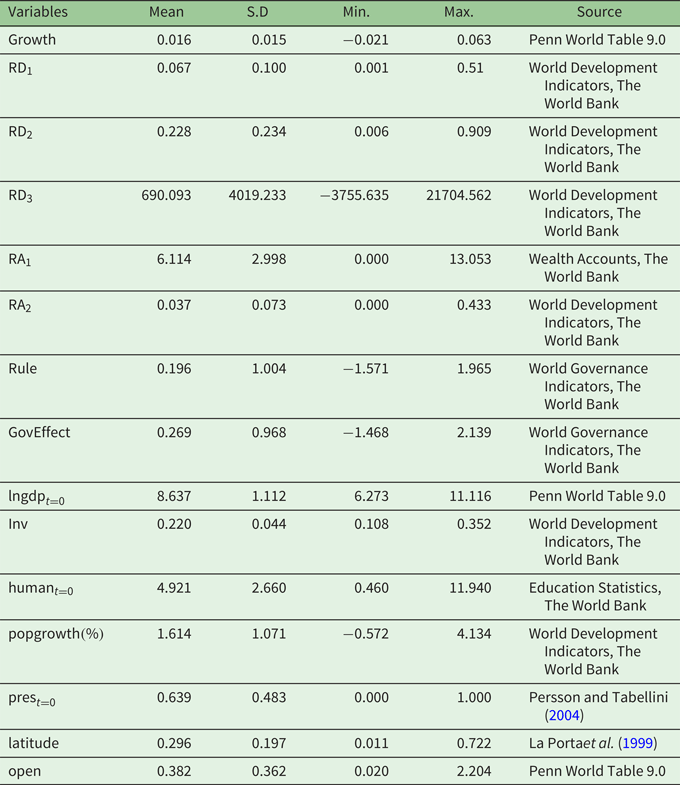
The summary statistics of our dataset are displayed in table 2.
Descriptive statistics

Notes : We provide here the sources where we actually obtain the data.${\rm RD}_1$ refers to the average GDP share of mineral exports. ${\rm RD}_2$
 is the average share of mineral exports in total export. ${\rm RD}_3$
 represents the net exports of mineral resources per worker. ${\rm RA}_1$
 is the log of subsoil asset per capita. ${\rm RA}_2$
 is the natural resources rents as a share of GDP. ${\rm Rule}$
 is the ‘Rule-of-law’ indicator while ${\rm GovEffect}$
 represents the government effectiveness. ${\rm lngdp}_{t=0}$
 is the log of real GDP in current PPP in 1980. ${\rm Inv}$
 is the investment-to-GDP ratio. ${\rm human}_t=0$
 is the average years of total schooling for people over 25 years old in 1980. ${\rm popgrowth}$
 represents the annual population growth rate. ${\rm pres}$
 is a dummy variable for the regime being Presidential (1) or Parliamentary (0). ${\rm open}$
 is a historical trade-openness variable.
3. Estimation strategy
3.1. The threshold regression model
We extend the linear model in Brunnschweiler and Bulte (Reference Brunnschweiler and Bulte2008) by introducing non-linearity. Wealso introduce additional regressors, namely human capital, investment, and population growth, to be consistent with the literature on growth. The main equation in the linear model of Brunnschweiler and Bulte (Reference Brunnschweiler and Bulte2008) is very similar to the following:Footnote 12

This regression can also be written as:

where

and

We look for a possible nonlinear effect of initial GDP per capita (i.e., in the starting period). The choice of the transition variable among the explanatory variables for threshold models is key. In many papers, this choice comes from economic theory. Here we appeal to the literature on convergence clubs to identify initial real GDP per capita as the threshold variable. The idea is to show that there are different growth trajectories, depending on initial GDP. We believe that these differences can be measured by the asymmetry of long-run GDP growth relative to initial GDP.Footnote 13 Hansen (Reference Hansen2000) uses initial GDP as the threshold variable in growth regression to distinguish multiple equilibria. This idea was inspired by Durlauf and Johnson (Reference Durlauf and Johnson1995), who suggest that cross-section growth may be determined by initial conditions. Clootens and Kirat (Reference Clootens and Kirat2017) uncover some evidence that countries do react differently to an increase in resource dependence or abundance by their initial level of GDP. We thus consider the following threshold-regression model:

where $\Psi ^{1}=(\beta_{0}^{1},\beta_{1}^{1},\beta_{2}^{1},\beta_{3}^{1},\beta_{4}^{1},\beta_{5}^{1},\beta_{6}^{1},\beta_{7}^{1})$ and $\Psi ^{2}=(\beta_{0}^{2},\beta_{1}^{2},\beta_{2}^{2},\beta_{3}^{2},\beta_{4}^{2},\beta_{5}^{2},\beta_{6}^{2},\beta_{7}^{2})$
 . The threshold parameter $q$
 is considered as unknown. It is convenient to rewrite (2) as:

where $\lambda =\Psi ^{1}-\Psi ^{2}$ . We want to estimate $\Psi ^{1}$
 , $\Psi ^{2}$
 and $q$
 if the null hypothesis of linearity is rejected, i.e., $H_{0}:\ \lambda =0$
 in equation (3).
We first examine this null hypothesis of linearity in equation (3), $H_{0}:\ \lambda =0$ . Without an a priori fixed value of $q$
 in regression (3), it is not easy to carry out statistical inference regarding $\lambda$
 . In this case $q$
 is a nuisance parameter that is not identified under the null hypothesis. Hansen (Reference Hansen1996) avoids this problem via a simulation technique producing a p-value statistic for the inference of $\lambda$
 . His approach does not require fixing an a priori value of $q$
 and allows for possible heteroskedasticity in (3). The calculation of the threshold estimate $\widehat {q}$
 uses the concentrated sum of squared errors function from (3):

and the threshold estimate $\widehat {q}$ is the value that minimizes $S(q)$
 :

where $\Gamma$ is a bounded set of elements of $\{gdp_{t=0,i},i=1,\ldots ,N\}$
 and can be approximated by a grid (see Hansen, Reference Hansen2000). Finally, the slope estimates in the threshold model (2) can be calculated using $\widehat {\Psi ^{2}}(\widehat {q})$
 and $\widehat {\lambda }(\widehat {q})$
 . Hansen (Reference Hansen2000) and Caner and Hansen (Reference Caner and Hansen2004) have also developed asymptotic-distribution theory for the threshold estimate $\widehat {q}$
 , and propose asymptotic confidence intervals by inverting the likelihood-ratio statistic. This approach also allows for possible heteroskedasticity in (3).
3.2. Dealing with endogeneity
Endogeneity is a central issue in threshold models. Threshold regression requires the exogeneity of regressors in equation (1), otherwise the estimates will be biased. In their paper, Brunnschweiler and Bulte (Reference Brunnschweiler and Bulte2008) identify a number of sources of endogeneity.Footnote 14 For instance, taking institutional quality and resource dependence as exogenous variables may lead to biased outcomes. Institutional quality might be linked to variables such as culture or other omitted variables that also determine growth. Moreover, resource dependence is not a proper explanatory variable in growth regressions. Resource dependence is, to a large extent, determined by the comparative advantage of the resource sector which in turn is determined by government choices. There is little doubt that those choices also determine growth.
Another concern is the exogeneity of the resource-abundance variables. We believe that ${\rm RA}_{1}$ may be reasonably thought of as exogenous. Obviously, the exploration and evaluation of resource stocks is a technologically-intensive process that is not independent of countries’ technological levels. Nevertheless, thanks to their economic potential, mineral deposits have been explored and estimated by large multinational firms regardless of the local conditions. While ${\rm RA}_{1}$
 is not free from criticism,Footnote 15 we believe that it constitutes a significant improvement with respect to the standard measure popularized by Sachs and Warner (Reference Sachs and Warner1995). Our second resource abundance variable $RA_{2}$
 is the natural resources rents as a share of GDP. It thus captures the actual rent that has been realized during the period. Broadly speaking, it is calculated as the difference between the resource price and the extraction cost, multiplied by extracted quantities. Finally, the scaling exercise supposes that the rent is divided by the GDP. To some extent, resource prices are determined on world markets and can be seen as exogenous.Footnote 16 The extraction costs are determined by the deposit quality. Clearly they can also be affected by the level of technology. However, mining deposits are often operated by large multinational firms that have access to the same technology. We thus believe that the unitary rent may reasonably be considered as exogenous. More suspicions can be put on the quantity extracted, and the scaling exercise, which are affected by government decisions. Still, while we acknowledge that this second resource-abundance variable is more prone to generate endogeneity issues, we consider it exogenous, and we use it mainly for robustness check purposes.
The literature has typically used three alternative instruments to control for the endogeneity bias introduced by institutions: latitude, the fraction of population speaking a Western-European language (Hall and Jones, Reference Hall and Jones1999) and the logarithm of settler mortality (Acemoglu et al., Reference Acemoglu, Johnson and Robinson2001). Latitude and the fraction of population speaking a Western language are measures of the extent to which the economy has been influenced by Western Europe, as this was the first area to introduce institutions supporting production. Nevertheless, these variables are not affected by current economic performance.Footnote 17
According to Acemoglu et al. (Reference Acemoglu, Johnson and Robinson2001), settler mortality is also a good instrument for institutions, as there were various types of colonization ranked from ‘extractive states’ to ‘neo-Europes’ (Crosby, Reference Crosby2004). The feasibility of settlements affected the colonization strategies such that ‘neo-Europes’ appeared where settler mortality was low. As past institutions are a major determinant of current institutional quality, settler mortality seems to be a good instrument for institutions. Here we use latitude to instrument institutions, as it is likely that mineral abundance promoted the establishment of extractive states.
We distinguish two institutional perspectives, following Brunnschweiler and Bulte (Reference Brunnschweiler and Bulte2008). First, institutions can be seen as persistent constitutional variables (Presidential vs. Parliamentary regimes, electoral rules, etc.) and refer to the ‘deep and durable’ characteristics of a society (Glaeser et al., Reference Glaeser, La Porta, Lopez De Silanes and Shleifer2004). On the other hand, institutions can also refer to the policy outcomes in property-rights enforcement, the fight against corruption and so on (Rodrik et al., Reference Rodrik, Subramanian and Trebbi2004). Our variables ${\rm Rule}$ and ${\rm GovEffect}$
 are of the second type, and may be endogenous when used in the second-step estimation. We therefore need to instrument them in a first step.
Brunnschweiler and Bulte (Reference Brunnschweiler and Bulte2008) show that deep and durable institutions can be used to instrument resource dependence. They use a dummy variable (for the country having a Presidential regime in the 1970s) as a proxy for institutions. Presidential regimes are often associated with public expenditures that are biased in favor of private interests (including the primary sector), as the decision maker does not have to rely on a stable majority. They also show that past trade openness is a good instrument for ${\rm RD}$ .Footnote 18
To avoid endogeneity issues in threshold estimation, we use here the predicted values of the ${\rm RD}$ and ${\rm Rule}$
 variables from instrumental equations (or first-step instrumental-variable estimations) instead of their observed values. The instrumentation procedure that we use here follows that in Brunnschweiler and Bulte (Reference Brunnschweiler and Bulte2008).
4. Results
We first check that there is evidence of a threshold effect associated with the initial level of GDP. We do so by carrying out the threshold test proposed by Hansen (Reference Hansen2000) on an instrumented version of equation (1):

where

and

In equation (4), $\widehat {\rm RD}$ and $\widehat {\rm Rule}$
 are the predicted values from the instrumental regressions (5) and (6).
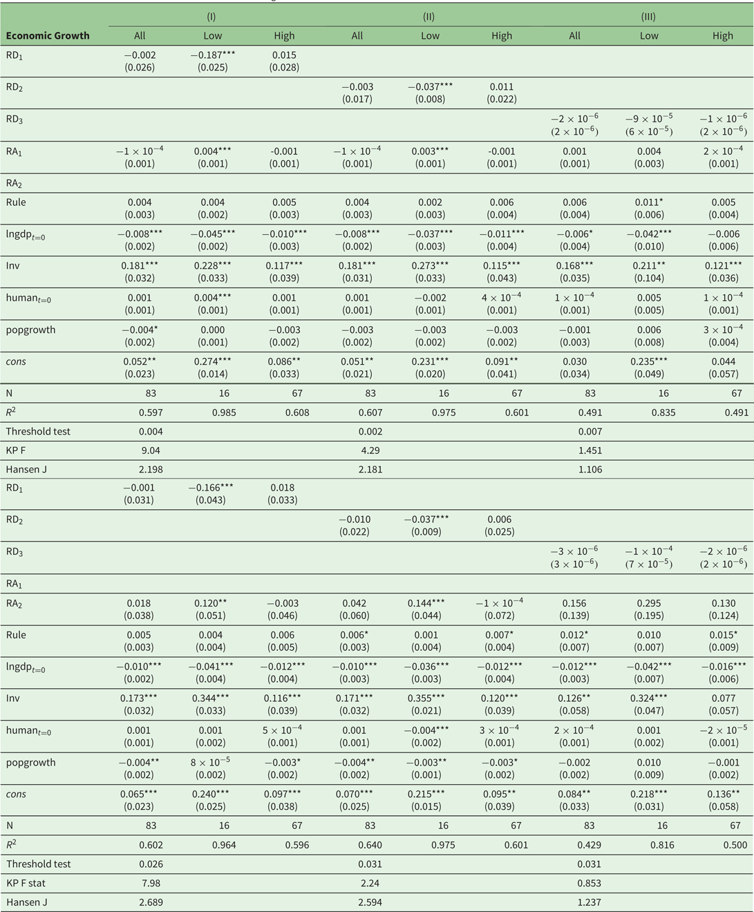
The non-linearity test strongly rejects the null hypothesis of linearity in favor of the alternative of a threshold effect at the 95 per cent confidence level in all six specifications reflecting various combinations of proxies for resource abundance and resource dependence. The bootstrapped p-values with 5,000 replications are reported in the bottom of table 3. There is then a threshold value of initial GDP that splits our sample into two subsamples, consistent with Clootens and Kirat (Reference Clootens and Kirat2017). Sample-splitting estimations should then be carried out for all specifications.
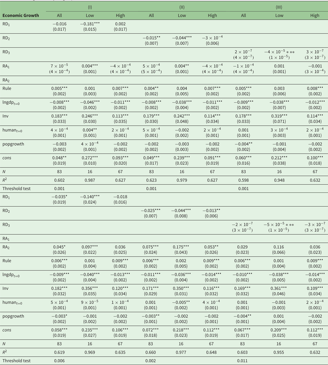
Estimation results of the effect of natural resources on growth

Robust standard errors in parentheses. *,** and *** refer respectively to the 10%, 5% and 1% significance levels. Models I and IV, II and V, III and VI use respectively${\rm RD}_1$ , ${\rm RD}_2$
 and ${\rm RD}_3$
 as proxies for resource dependence. Models I, II and III use ${\rm RA}_1$
 to proxy for resource abundance, while models IV, V and VI use ${\rm RA}_2$
 .${\rm RD}_1$
 refers to the average GDP share of mineral exports. ${\rm RD}_2$
 is the average share of mineral exports in total export. ${\rm RD}_3$
 represents the net exports of mineral resources per worker. ${\rm RA}_1$
 is the log of subsoil asset per capita. ${\rm RA}_2$
 is the natural resources rents as a share of GDP. ${\rm Rule}$
 is the ‘Rule-of-law’ indicator. ${\rm lngdp}_{t=0}$
 is the log of real GDP in current PPP in 1980. ${\rm Inv}$
 is the investment-to-GDP ratio. $Human_t=0$
 is the average years of total schooling for people over 25 years old in 1980. ${\rm popgrowth}$
 represents the annual population growth rate. ${\rm pres}$
 is a dummy variable for the regime being Presidential (1) or Parliamentary (0). ${\rm open}$
 is a historical trade-openness variable. ${\it Cons}$
 is the constant of regression. The first-step results for the main regressions appear in apendix A.2. The threshold test line reports p-values against the null of no threshold. We report the Kleibergen-Paap rk Wald F statistic (test of weak identification) and the Hansen J statistic (test of overidentifying restrictions).
Table 3 presents the estimation results for the threshold growth models. It reports the estimation results of six different specifications reflecting various combinations of proxies for resource abundance and resource dependence. Table 3 also contains the estimation results from the corresponding linear models, and underlines the non-relevancy of estimates when non-linearity is not taken into account. For each specification in table 3, the first column reports the IV estimates of the linear model while the second and third columns report respectively those of the low regime and the high regime of the corresponding threshold model. The estimated initial GDP per capita thresholds are robust to change in the resource-dependence and resource-abundance proxies and equal $1,928.48 (current PPP in 1980) in all specifications.
The instruments are exogenous according to the Hansen J overidentification test statistic, which is robust to heteroskedasticity. The Hansen J stat is below the $\chi ^{2}$ critical value of $3.84$
 for all six specifications. Although the instruments are not perfect, the Kleibergen-Paap F statistics for weak identification test are much more favorable in specifications (I) and (IV). The instruments predict the average GDP share of mineral exports or ${\rm RD}_{1}$
 , much better than the other metrics of resource-dependence ${\rm RD}_{2}$
 and ${\rm RD}_{3}$
 . The Shea's partial $R^{2}$
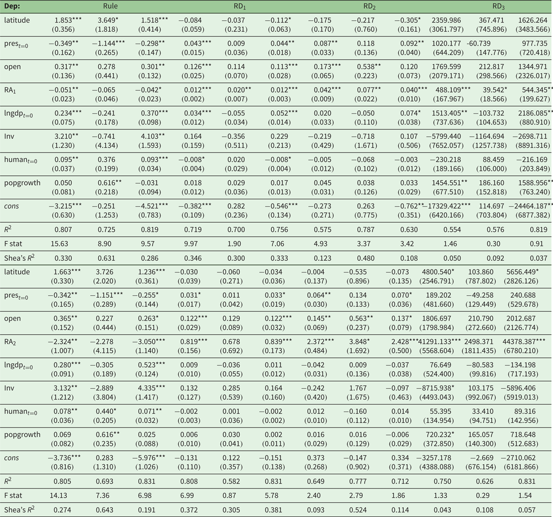
 reported in table A2 confirm the conclusions of these diagnostic statistics. The excluded instruments explain a significant part of the endogenous variables ${\rm Rule}$
 and ${\rm RD}$
 in most cases, with the exception of ${\rm RD}_{3}$
 for which instruments are likely to be weak.
The results in table 3 support the insights in Clootens and Kirat (Reference Clootens and Kirat2017) regarding the need for sample splitting: poor and rich countries (defined using the method in Hansen (Reference Hansen2000)) do not react in the same way with respect to natural resources.Footnote 19 In low-income economies, resource dependence is a curse that reduces growth possibilities, while resource abundance remains a blessing. In our favorite specification (I) with regard to the relevance of instruments, it appears that a one percentage point rise in the GDP share of mineral exports leads to a fall of 0.187 percentage points in growth, all things being equal. However, an increase of one unit in the logarithm of subsoil assets is associated with higher growth of about 0.4 percentage points, all things being equal. The negative sign of the estimated parameter associated to initial GDP per capita reflects catch-up. Finally, human capital and investments affect growth positively. Indeed, an increase of one percentage point in the share of GDP devoted to investment increases growth by 0.228 percentage points while an increase of one year of total schooling for people over 25 in 1980 increases growth by 0.4 percentage points, all things being equal.
In high-income economies, growth is neither determined by dependence nor abundance. The GDP share of investment seems to increase growth while we also find a catch-up effect.
These results seem robust when we change the resource dependence variable for the total export share of mineral exports (${\rm RD}_{2}$ ). However, when we use the third mineral dependence indicator ${\rm RD}_{3}$
 (the net exports of minerals per worker), we find no significant impact of either abundance or dependence on growth. Still, the signs of the estimates are consistent with previous estimations. The non-significance of parameters is probably due here to the weakness of instruments. The corresponding Shea's partial R squared are very low and reported to be around 0.10 (see table A2). According to van der Ploeg and Poelhekke (Reference van der Ploeg and Poelhekke2010), this implies noisy 2SLS first-stage estimates, leading to inflation of the second-stage standard errors by $0.1^{-0.5}\approx 3.16$
 . This may mean that the estimated coefficients associated with the net exports of minerals per worker variable is much more significant than suggested.
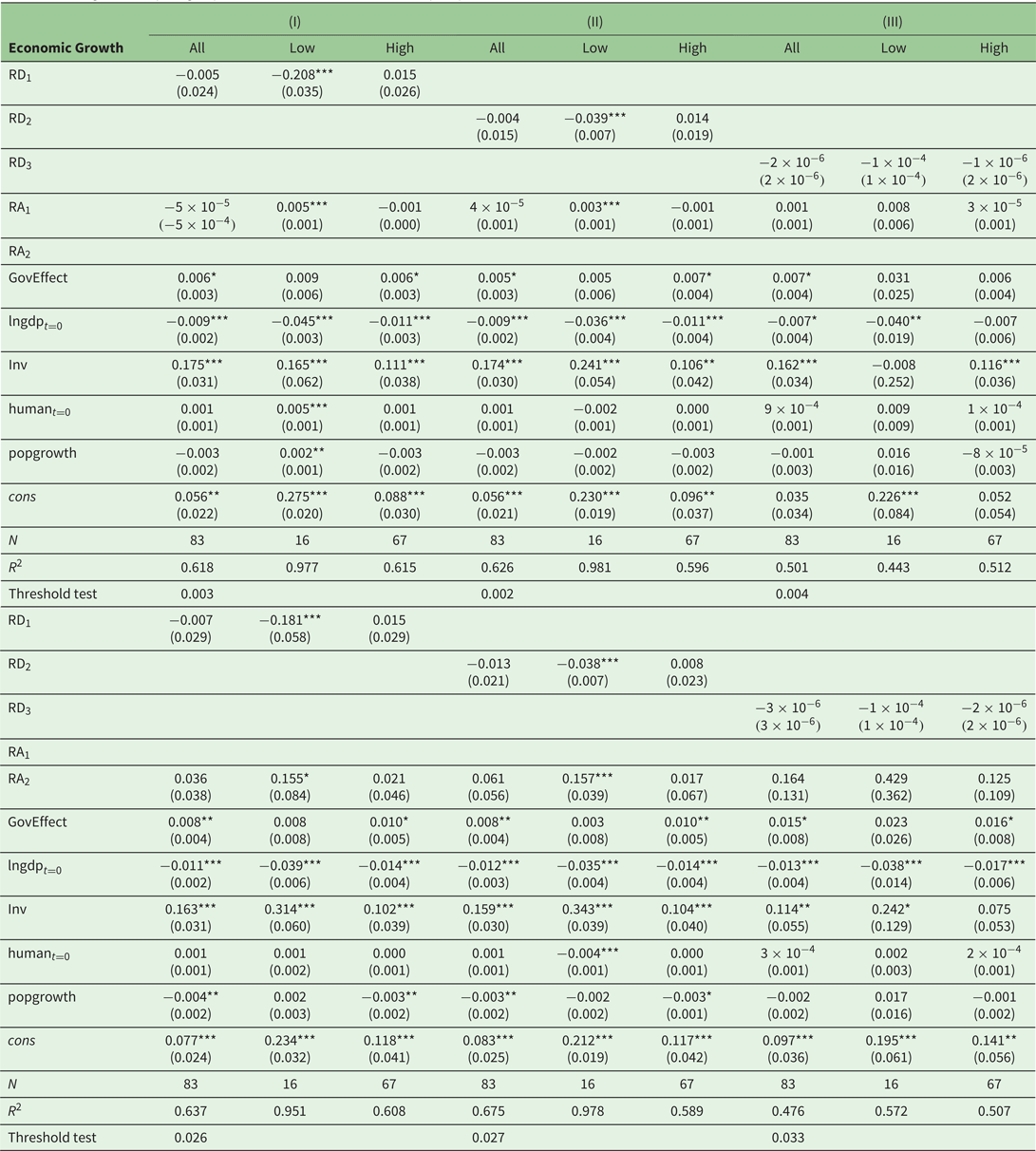
The results remain consistent when we introduce changes in variables proxying for resource abundance. Considering the natural resource rent as a share of GDP instead of the logarithm of subsoil-asset natural capital per capita does not significantly change the estimation results. Our results are also robust to the use of an alternative institutional quality variable, namely the government effectiveness (see appendix). Finally, we also propose the OLS estimates in the appendix. Using OLS in place of 2SLS does not strongly change the results except for specifications (III) and (VI) which suggest some room for a dependence curse also when we use ${\rm RD}_{3}$ as the resource-dependence indicator.
The consistency of our results requires the exogeneity of the threshold variable. This point is crucial. Indeed, Caner and Hansen (Reference Caner and Hansen2004) suggested the use of a 2SLS estimator to correct the endogeneity of the explanatory variables when the threshold variable is necessarily exogenous as is the case in our model. Yu (Reference Yu2013), however, shows that even in the case where the threshold variable is exogenous the 2SLS estimator of Caner and Hansen (Reference Caner and Hansen2004) may be inconsistent. Yu (Reference Yu2013) and Yu and Phillips (Reference Yu and Phillips2018) give examples where the true relationship between the endogenous, right-hand-variables and their instrumental variables are non-linear but mistakenly considered as linear to support this result. To overcome this issue, Yu and Phillips (Reference Yu and Phillips2018) suggest a non-parametric estimator of the threshold which is, unfortunately, data consuming. For these reasons, special attention should be paid to the instrumental equations to ensure that they are well specified. Fortunately, the estimated results in table A2 show that the instrumental equations are well specified and have good statistical properties including high explanatory power (High R-squared and partial R squared of Shea) and high significance levels of the estimated parameters, which move us away from the particular case that invalidates the 2SLS estimator.
The results for mineral dependence contradict one of the principal results in Brunnschweiler and Bulte (Reference Brunnschweiler and Bulte2008):Footnote 20 we find that with sample splitting, resource dependence matters for the growth of developing economies. Initial GDP per capita is typically introduced in growth regressions to reflect catch-up. Here, this variable also acts as the sample-splitting variable to take into account the heterogeneity of countries with respect to their stage of development. Implicitly, by choosing this variable to split the sample, we suppose that countries on each side of the threshold share common properties in a way that is determined by their initial level of development. Notably, we believe that a country with high income per capita in 1980 is probably a country with a market-friendly environment in 1980: a more-educated population, developed financial markets, sufficient trade openness, good institutional quality, a high level of investment, and so on. These shared characteristics help high-income economies compensate for the negative impact that natural resource dependence may have on economic performance. For example, the probability of civil conflict falls with education. Moreover, the potential cost that will be incurred by the failure of rebellion is higher in high-income economies. Developed markets may also reduce rebellion for grievance reasons, and help to absorb shocks to resource prices. Greater (unobserved) institutional quality implies less corruption and misappropriation of public revenue. The Dutch disease or other crowding-out mechanisms associated with natural resources are easier to counter with appropriate economic policy when markets are developed.
As we may think that resource abundance generates dependence, we would like to calculate the net effect of natural-resource abundance on economic growth. We can do so using our first-stage IV estimates (see appendix). We conclude that the net effect of resource abundance is such that a one unit rise in the logarithm of subsoil assets generates an average increase in growth of about $0.026$ and $0.015$
 percentage points in low-income economies when one considers specifications (I) and (II) respectively. We should nevertheless be cautious regarding these figures, and believe that there is some potential for a resource-dependence curse. However, if resource abundance does improve growth, there is no universal resource curse: resource abundance does not necessarily reduce growth, even if greater resource dependence does hamper growth in low-income economies.
5. Conclusion
This paper has added to the work of Brunnschweiler and Bulte (Reference Brunnschweiler and Bulte2008) by improving the treatment of heterogeneity between countries. We notably use the sample-splitting method in Hansen (Reference Hansen2000) on an updated data set. One of the main results in Brunnschweiler and Bulte (Reference Brunnschweiler and Bulte2008) is affected by the sample split: resource dependence negatively affects development in low-income countries (but has no effect in high-income countries). We acknowledge that this result is not independent of the choice of the threshold variable. While our method allows us to test for and estimate the value of the threshold without any subjective considerations, we still have to choose the threshold variable.
The natural resource effect on growth is dependent on the growth regime a country belongs to, which is in turn determined by the level of initial GDP. Initial GDP is highly correlated with initial levels of institutional quality, trade-openness, human capital, market development, etc. We believe that high-income economies share a number of common properties that allow them to limit the negative effects of natural resources on growth. We thus argue that developing education, financial markets and institutions may restrict the negative influence of resource dependence on growth. Moreover, since resource dependence results from economic choices, it can be avoided by an appropriate diversification policy.
To summarize, we highlight that it is difficult to promulgate universal laws, such as that natural-resource abundance is a blessing or a curse. We argue that while, on average, resource abundance favors growth in low-income economies, there does also exist some evidence for a resource-dependence curse.
Acknowledgements
The authors are grateful to two anonymous referees and the editors for their helpful comments. Comments by Alain Desdoigts on an earlier version of this work were also very useful. The authors are also indebted to conference participants for comments received in response to presentations of this paper at the EAERE 2017 in Athens; INFER 2017 in Bordeaux; AFSE 2017 in Nice; and GDRI IDE 2016 in Clermont-Ferrand. This paper has been partly funded by the Agence Nationale de la Recherche (France) under grants Labex VOLTAIRE (ANR-10-LABX-100-01) and ANR-17-EURE-0020. Any remaining shortcomings are the authors’ responsibility.
Appendix
A.1 List of countries
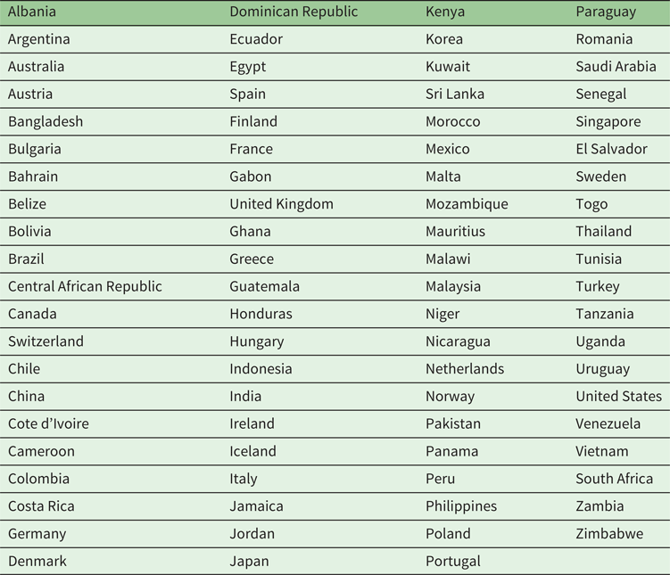
Table A1 reports the list of countries included in our regressions. The unique criteria of country selection was data availability. We keep all the countries for which we had a complete set of data.
List of countries

A.2 First-stage regressions
Table A2 reports first-stages estimations of our main IV regression.
First-stages estimations

A.3 The OLS regression
If there are no endogeneity problems in the data, a simple OLS regression is more effcient than a 2SLS regression. We believe that there are good reasons to suspect endogeneity and use 2SLS. Nevertheless, robustness checks using OLS are of interest. The threshold test concludes for the rejection of the null hypothesis of linearity in all specifications. Table A.3 presents the results of the threshold OLS estimations by regime.
OLS regressions by subgroups

The results confirm those above: RD has a negative impact on growth while RA is a blessing for low-income economies. There is still a catch-up effect in this group, while Inst becomes significant, which is as expected as OLS implies an efficiency gain with respect to IV in the absence of endogeneity. Neither natural-resource abundance nor dependence affect growth in developed economies.
A.4 Alternative institutional quality measure
In table A4, we use an alternative proxy for institutional quality, namely the government effectiveness (see Kaufmann et al., Reference Kaufmann, Kraay and Mastruzzi2009).
IV regressions by subgroups, alternative index for institutional quality