
1. Introduction
Ice tanks and laboratory experiments in them are used to design ships and offshore structures for polar regions and to study their performance in icy waters. In experiments with a ship model, a model is towed in a lead of open water made in the ice cover of the tank. The ship model experiments in an ice tank are more complicated and expensive than experiments in a water tank. Such experiments should be carefully designed and prepared. Characteristics of the ice tank with a lead should be examined before the experiments, in particular, in term of flexural-gravity waves propagating along the tank. Dispersion relations of these waves, their phase and group speeds should be investigated with particular focus on the so-called critical speeds of the waves, where the phase and group speeds are equal to each other. If a ship moves in a lead at a critical speed then the ice deflections and the ship resistance are extreme.
In the polar regions such leads can be natural caused by various natural forces including wind, wave and current, etc. (Squire Reference Squire2007) or can be made by an icebreaker. Leads are important waterways in the polar regions. The leads may be found or can be made in some northern rivers in springtime. Leads on the rivers can prevent floodings.
The problem of linear waves in the presence of an ice lead has received considerable attention over the last decades (Squire Reference Squire2007, Reference Squire2011). Such waves can arrive at an ice lead from any direction. For waves propagating perpendicular to the ice lead, Chung & Linton (Reference Chung and Linton2005) studied the flexural-gravity waves in two-dimensional formulations using the residue calculus technique. It was found that there was an infinite number of frequencies at which the waves transmit without any loss from one side of the open water lead to the other. Shi, Li & Wu (Reference Shi, Li and Wu2019) investigated two-dimensional waves scattering by multiple polynyas using a wide spacing approximation method. For waves propagating into the ice lead obliquely, Williams & Squire (Reference Williams and Squire2006) considered a more general case of flexural-gravity waves propagating into three floating Euler–Bernoulli thin elastic plates with different thicknesses. There were no gaps between the plates and the edges of the plates were free of bending stresses and shear forces. The thickness of the central plate can be reduced to zero, so waves propagating through an ice lead can be dealt with directly. Porter (Reference Porter2018) focused on the same problem but for an infinite water depth. He confirmed existence of edge waves, which are localized near the ice edges and do not penetrate the ice sheet deeply. For waves propagating along an ice lead, Marchenko (Reference Marchenko1997) obtained the dispersion relations within the shallow water approximation, where the ice cover was modelled as either rigid plates or as thin semi-infinite elastic plates.
The problems of wave/ice sheet interaction in confined regions, such as rivers and channels, also received attention. In hydraulic engineering the problems of waves propagating in ice-covered channels are usually considered as one dimensional without account for conditions of the ice cover connection with the channel walls. Daly (Reference Daly1993) studied an unsteady flow in a rectangular ice-covered channel by using three linearised governing equations. These equations described the mass and momentum conservation and the motion of the ice cover. Daly (Reference Daly1993) found that for waves longer than 20 characteristic lengths of the ice, the wave propagation is not affected by the presence of the ice cover. Daly (Reference Daly1995) further investigated the bending stresses in the ice cover and found that the bending stresses are maximum for flexural-gravity waves, the length of which is close to  $2{\rm \pi} l$, where
 $l$ is the characteristic length of the ice cover. Xia & Shen (Reference Xia and Shen2002) derived a one-dimensional weakly nonlinear fifth-order KdV equation for shallow water wave propagation in a uniform channel with a floating ice cover. They proved that the cnoidal waves could generate sufficient stresses to fracture the ice cover. Beltaos (Reference Beltaos2004) studied one-dimensional long waves of small amplitudes propagating along an ice channel with transverse cracks and intervals of open water. He concluded that ‘a truncated low-amplitude wave, which is a wave propagating past an edge (or crack) into an undisturbed region, produces generally higher bending stresses than does an infinitely long wave propagating under an edgeless cover. However, the maximum possible stress is the same for both cases, and occurs at the same dimensionless wavenumber of 1, or where the wavelength is equal to about six times the characteristic length of the ice cover’. A numerical model was derived by Nzokou et al. (Reference Nzokou, Morse, Robert, Richard and Tossou2011) to simulate the interaction between dam break waves and ice-covered channel using the one-dimensional Saint-Venant equations representing mass and momentum conservation for water flowing in an ice-covered channel and the one-dimensional ‘elastic foundation beam equation of a floating ice sheet including the terms representing vertical acceleration and longitudinal shear stress applied to the bottom of the ice sheet by the water flowing under it’. They found that, for the conditions of their calculations, ice stiffness had no significant effect on the celerity of waves and their attenuation for waves longer than
 $400$ m. For short waves (
 $50$ m), the decrease in celerity due to stiffness was found to be
 $6\,\%$ and the additional attenuation as high as
 $20\,\%$. Fuamba, Bouaanani & Marche (Reference Fuamba, Bouaanani and Marche2007) studied dam break wave propagation in a channel partially covered with ice between two consecutive dams. One-dimensional flow in the open water part of the channel and under the rigid ice cover were calculated numerically without account for the ice deflection. Then the one-dimensional pressure wave under the rigid cover was applied to a finite element model of flexible ice clamped to the channel side walls. The numerical results were in good agreement with the results of laboratory tests, which confirmed the approximation of the rigid ice and the pressure wave propagating under the ice cover. The bending stresses were found to be maximum at the walls of the channel. It was argued that the connection of the ice with the walls was important for the stress distribution in the ice cover. Nzokou, Morse & Quach-Thanh (Reference Nzokou, Morse and Quach-Thanh2009) numerically studied a given incoming one-dimensional water wave propagating in an ice-covered channel, where the ice cover was modelled as a two-dimensional ice sheet. The ice sheet was assumed to be clamped to or detached from the channel walls. It was found that there was a high stress concentration near the walls due to the fixed boundary conditions. However, close to the central axis of the channel, the calculated stresses turned out to be similar in value with those obtained using the one-dimensional approximation, that is, without connections of ice cover with the channel walls being considered. Guyenne & Parau (Reference Guyenne and Parau2017) performed two-dimensional numerical simulations of long nonlinear waves propagating in fragmented sea ice featuring floes and leads. It was observed that gravity-dominated short waves are widespread in areas of open water between floes.
Three-dimensional flexural-gravity waves propagating in the ice-covered channel attracted researchers’ attention only recently. Korobkin, Khabakhpasheva & Papin (Reference Korobkin, Khabakhpasheva and Papin2014) investigated hydroelastic waves propagating along a rectangular frozen channel and their dispersion relations for the continuous ice sheet clamped to the walls of the channel. The linear theory of hydroelasticity and the normal mode method were used. The wave profiles across the channel and the strain distributions in the ice sheet were analysed. It was found that the maximum strains were achieved at the walls for longer waves, and at the centreline of the channel for shorter waves. Batyaev & Khabakhpasheva (Reference Batyaev and Khabakhpasheva2015) studied a similar problem but with free edge conditions between the ice cover and the channel walls. Ren, Wu & Li (Reference Ren, Wu and Li2020) developed an efficient procedure to the problem of waves propagating in a rectangular channel fully covered by the ice sheet with or without a longitudinal crack in the ice cover. Various edge conditions between the ice sheet and the channel walls were considered. It was shown that the first natural frequency of waves propagating in a channel covered by continuous ice sheet, corresponding to different edge conditions between the ice cover and the channel walls, were very close to each other. For waves propagating in a fully ice-covered channel with an infinite longitudinal crack in the ice cover, the effects of the position of the crack on dispersion relations, wave profiles and strain distributions were investigated. It was found that when the crack approaches a channel wall, the results tend to those for the continuous ice sheet with a free edge between the channel wall and ice sheet.
In the present work we focus on waves propagating along an ice channel with a lead of open water in the ice cover. The presence of a lead significantly changes the characteristics of the propagating waves. The lead is symmetric about the centreline of the ice channel. The identical ice sheets on both sides of the lead are clamped to the walls of the channel. The ice sheets are modelled as either thin elastic plates of constant thickness or as rigid plates. The deflection of the ice sheet is described by the elastic plate equation.
The paper is organized as follows. The formulation of the problem is given in § 2. The normal mode method is applied to solve the problem in § 3. The coupled problem of hydroelastic waves is reduced to a linear system of algebraic equations. The same problem but within the rigid ice model is studied in § 4. Numerical algorithms and their validations are presented in § 5. Numerical results are provided in § 6 for the dispersion relations of the hydroelastic waves, their phase speeds and critical speeds, as well as the profiles of these waves across the channel. Conclusions are drawn and future work is discussed in § 7.
2. Formulation of the problem
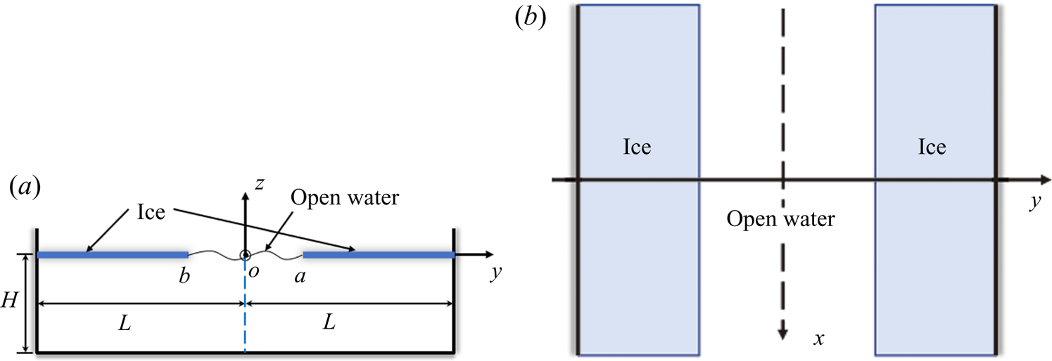
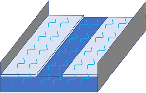
Linear sinusoidal waves propagating along an ice channel with an open water lead in the ice cover are studied. The configuration of the ice tank is shown in figure 1. The channel, in the Cartesian coordinate system  $Oxyz$, is of rectangular cross-section with width
 $2L$,
 $-L\lt y\lt L$, depth
 $H$,
 $-H<z<0$ and infinite extent in the
 $x$-direction. The ice cover floating on the water surface is with an open water lead which corresponds to the interval
 $b<y<a$. The ice is modelled as a thin elastic plate of constant thickness
 $h$. The mass of the ice per unit area is
 $m$ and the ice rigidity is
 $D=Eh^3/[12(1-\nu ^2)]$, with
 $E$ and
 $\nu$ being the Young's modulus and Poisson's ratio of the ice sheet. Within the linear theory of hydroelasticity, the elevation of the upper boundary of the flow region,
 $z=w(x,y,t)$, is governed by the equations,
 \begin{equation} \left. \begin{array}{c@{}} m w_{tt}+D\nabla^4 w=p(x,y,0,t) \quad ({-}L\lt y\lt b,a\lt y\lt L, -\infty\lt x\lt \infty), \\ p(x,y,0,t)=0 \quad (b\lt y\lt a, -\infty\lt x\lt \infty), \end{array} \right\} \end{equation}
where  $p(x,y,0,t) =-\rho \varphi _t(x,y,0,t) -\rho g w(x,y,t)$ is the hydrodynamic pressure on the upper boundary of the flow region,
 $\rho$ is the water density,
 $g$ is the gravitational acceleration and
 $\varphi (x,y,z,t)$ is the velocity potential of the flow. Note that
 $w(x,y,t)$ is not continuous at
 $y=b$ and
 $y=a$. The elevation of the free surface and the deflection of the ice cover are, in general, different at the ice edges. The ice edges are free of stresses and shear forces,
 \begin{equation} \dfrac{\partial ^2 w}{\partial y^2} + \nu\dfrac{\partial ^2 w}{\partial x^2} =0,\quad \dfrac{\partial ^3 w}{\partial y^3}+(2-\nu )\dfrac{\partial ^3 w}{\partial x^2 \partial y} =0 \quad (y=b^-,a^+, -\infty<x<\infty), \end{equation}
where  $y=b^{-}$ and
 $y=a^{+}$ imply that we approach the edges from the ice. The other edges of the ice plates,
 $y=\pm L$, are clamped (frozen) to the vertical walls of the channel,
 \begin{equation} w=0, \quad \dfrac{\partial w}{\partial y}=0 \quad (y={\pm} L). \end{equation}
The velocity potential  $\varphi (x,y,z,t)$ satisfies the Laplace equation in the flow region,
 \begin{equation} \nabla^2\varphi=0 \quad (|x|\lt \infty, \ |y|\lt L,\ -H\lt z\lt 0), \end{equation}
and the boundary conditions,
 \begin{equation} \dfrac{\partial \varphi}{\partial y}=0 \quad (y={\pm} L), \quad \dfrac{\partial \varphi}{\partial z}=0 \quad (z={-}H), \quad \dfrac{\partial \varphi}{\partial z}=\dfrac{\partial w}{\partial t} \quad (z=0), \end{equation}
where the third equation is linearised. The waves propagating along the ice channel correspond to the solutions of the problem (2.1)–(2.5a–c) in the form
 \begin{equation} w=F(y)\cos(kx-\omega t), \quad \varphi=\omega\varPhi(y,z)\sin(kx-\omega t), \end{equation}
where  $k$ is the wavenumber and
 $\omega$ is the wave frequency, the function
 $F(y)$ describes the wave profile across the channel. Along the channel the wave is sinusoidal. We shall determine the dispersion relations between the wavenumber
 $k$ and the wave frequencies
 $\omega _n(k)$, and the corresponding wave profiles
 $F_n(y)$, where
 $\omega _{n+1}(k)>\omega _n(k)$ and
 $n\geq 1$.
(a) The front view of the channel with the ice sheets and the open water lead. (b) The top view of the channel.

Substituting (2.6a,b) in (2.1)–(2.5a–c), we arrive at the boundary value problem with respect to the function  $F(y)$,
 \begin{align} \left. \begin{array}{c@{}} D[F^{iv}-2k^2 F''+k^4 F]-m\omega^2 F+\rho gF=\rho\omega^2 \varPhi(y,0) \quad ({-}L\lt y\lt b,a\lt y\lt L), \\ \rho g F=\rho\omega^2 \varPhi(y,0) \quad (b\lt y\lt a), \end{array} \right\} \end{align}
 \begin{gather} F=F'=0 \quad (y={\pm} L), \quad F''-\nu k^2 F=0, \quad F'''-(2-\nu )k^2F'=0 \quad (y=b,y=a). \end{gather}
The first equation in (2.7) is the fourth-order ordinary differential equation for  $F(y)$ in the intervals
 $-L<y<b$ and
 $a\lt y\lt L$ with four boundary conditions (2.8a–c) in each interval. The potential
 $\varPhi (y,z)$ on the right-hand side of (2.7) is the solution of the boundary problem, which follows from (2.4) and (2.5a–c),
 \begin{gather} \varPhi_{yy}+\varPhi_{zz}-k^2\varPhi=0 \quad (|y|\lt L,\ -H\lt z\lt 0), \end{gather}
 \begin{gather}\varPhi_y=0 \quad (y={\pm} L), \quad \varPhi_z=0 \quad (z={-}H), \quad \varPhi_z=F(y) \quad (z=0). \end{gather}
On the upper boundary of the channel, the pressure caused by the wave (2.6a,b) is given by
 \begin{equation} \left.\begin{array}{c@{}} p(x,y,0,t)={-}\rho\varphi_t-\rho g w(x,y,t)=P(y)\cos(kx-\omega t), \\ P(y)=\rho\omega^2\varPhi(y,0)-\rho g F(y). \end{array}\right\} \end{equation}
We shall determine non-trivial solutions of the homogeneous boundary problems (2.7)–(2.10a–c) and the corresponding frequencies  $\omega _n(k)$ within the model of elastic ice (2.7), (2.8a–c) and the model of rigid ice, where
 $F(y)=0$ in
 $-L<y<b$ and
 $a\lt y\lt L$.
3. Waves within the elastic ice model
The ice deflection is presented by superposition,
 \begin{equation} F(y)= \left\{ \begin{array}{@{}ll} \displaystyle \sum_{n=1}^\infty G_n\chi_n(y) & ({-}L\lt y\lt b), \\ \displaystyle \sum_{n=1}^\infty F_n\psi_n(y) & (a\lt y\lt L). \end{array} \right. \end{equation}
Substituting (3.1) in the first equation of (2.7) without the inhomogeneous term and using the boundary conditions (2.8a–c), we arrive at the eigenvalue problem of the modes  $\chi _n(y)$ and
 $\psi _n(y)$,
 \begin{gather} \left.\begin{array}{ll@{}} \displaystyle \left(\dfrac{\mathrm{d}^2}{\mathrm{d} y^2}-k^2\right)^2 \chi_n = \beta_n^4\chi_n \quad ({-}L<y<b),\\ \chi_n''(b)=\nu k^2\chi_n(b), \quad \chi_n({-}L)=0, \\ \chi_n'''(b)=(2-\nu)k^2\chi_n'(b), \quad \chi_n'({-}L)=0, \end{array}\right\} \end{gather}
 \begin{gather}\left. \begin{array}{l@{}} \displaystyle \left(\dfrac{\mathrm{d}^2}{\mathrm{d} y^2}-k^2\right)^2 \psi_n = \lambda_n^4\psi_n \quad (a\lt y\lt L),\\ \psi_n''(a)=\nu k^2\psi_n(a), \quad \psi_n(L)=0, \\ \psi_n'''(a)=(2-\nu)k^2\psi_n'(a), \quad \psi_n'(L)=0, \end{array} \right\} \end{gather}
with the corresponding eigenvalues  $\beta _n$ and
 $\lambda _n$, which are obtained in Appendix A. The modes
 $\chi _n(y)$ and
 $\psi _n(y)$ are orthogonal and normalised,
 \begin{equation} \int_{{-}L}^b \chi_n(y)\chi_m(y) \,\mathrm{d} y = \delta_{nm}, \quad \int_a^L \psi_n(y)\psi_m(y) \,\mathrm{d} y = \delta_{nm}, \end{equation}
where  $\delta _{nn}=1$ and
 $\delta _{nm}=0$ for
 $n\neq m$. The coefficients
 $G_n$ and
 $F_n$ in (3.1) are unknown in advance and should be determined using (2.7)–(2.10a–c).
Equations (2.7), (2.11) and (3.2) provide the pressure  $P(y)$ on the ice–water interface,
 \begin{equation} P(y)= \left\{\begin{array}{@{}ll} \displaystyle \sum_{n=1}^\infty G_n\chi_n(y)[{-}m\omega^2+D\beta_n^4] & ({-}L\lt y\lt b), \\ \displaystyle\sum_{n=1}^\infty F_n\psi_n(y)[{-}m\omega^2+D\lambda_n^4] & (a\lt y\lt L). \end{array}\right. \end{equation}
In the lead,  $b<y<a$, the pressure is zero,
 $P(y)=0$. The kinematic condition,
 $\varPhi _z(y,0)=F(y)$, makes it possible to transform (2.7) to the following boundary condition on the upper boundary
 $z=0$:
 \begin{equation} \dfrac{\partial \varPhi}{\partial z}-\dfrac{\omega^2}{g}\varPhi= \left\{\begin{array}{@{}ll} \displaystyle\sum_{n=1}^\infty G_n\chi_n(y)\left[\dfrac{m\omega^2}{\rho g}-\dfrac{D\beta_n^4}{\rho g}\right] & ({-}L\lt y\lt b),\\[14pt] 0 & (b\lt y\lt a),\\ \displaystyle\sum_{n=1}^\infty F_n\psi_n(y)\left[\dfrac{m\omega^2}{\rho g}-\dfrac{D\lambda_n^4}{\rho g}\right] & (a\lt y\lt L). \end{array} \right. \end{equation}
The solution of the problem (2.9)–(2.10a–c), where the condition at  $z=0$ is changed to (3.5), can be written as
 \begin{equation} \varPhi(y,z)=\sum_{n=1}^\infty \varPhi_n(y,z), \end{equation}
where the potentials  $\varPhi _n(y,z)$,
 $n\geq 1$, are the solutions of the following boundary value problem:
 \begin{gather} \varPhi_{n,yy}+\varPhi_{n,zz}-k^2\varPhi_n=0 \quad (|y| \lt L,\ -H\lt z\lt 0), \end{gather}
 \begin{gather}\varPhi_{n,y}=0 \quad (y={\pm} L), \quad \varPhi_{n,z}=0 \quad (z={-}H), \end{gather}
 \begin{gather}\dfrac{\partial \varPhi_n}{\partial z}-\dfrac{\omega^2}{g}\varPhi_n= \left\{\begin{array}{@{}ll} G_n\chi(y) \dfrac{m\omega^2-D\beta_n^4}{\rho g} & (z=0, -L\lt y\lt b), \\ 0 & (z=0, b\lt y\lt a),\\ F_n \psi_n(y) \dfrac{m\omega^2-D\lambda_n^4}{\rho g} & (z=0, a\lt y\lt L). \end{array} \right. \end{gather}
The kinematic condition,  $\varPhi _z(y,0)=F(y)$, where
 $-L\lt y\lt L$, (3.1) and (3.6) provide the equation
 \begin{equation} \displaystyle\sum_{n=1}^\infty \dfrac{\partial \varPhi_n}{\partial z}=\left\{\begin{array}{@{}ll} \displaystyle \sum_{n=1}^\infty G_n\chi(y) & ({-}L\lt y\lt b), \\ \displaystyle\sum_{n=1}^\infty F_n \psi_n(y) & (a\lt y\lt L), \end{array}\right. \end{equation}
which leads to the infinite linear system of equations for the coefficients  $G_n$ and
 $F_n$,
 \begin{equation} \left\{\begin{array}{@{}l} \displaystyle \sum_{n=1}^\infty \int_{{-}L}^{b}\dfrac{\partial \varPhi_n}{\partial z} \chi_{k}(y) \,\mathrm{d} y = G_n \delta_{kn} \quad ({-}L\lt y\lt b),\\ \displaystyle \sum_{n=1}^\infty \int_{a}^{L}\dfrac{\partial \varPhi_n}{\partial z} \psi_{k}(y) \,\mathrm{d} y = F_n \delta_{kn} \quad (a\lt y\lt L), \end{array}\right. \end{equation}
using the orthogonality relation (3.3a,b). Finally, we solve the homogeneous equation (3.11) to determine the coefficients  $G_n$ and
 $F_n$.
In the present study we limit ourselves to the open water leads which are symmetric with respect to the central line of the channel,  $-b=a$, and symmetric waves,
 $w(x, -y, t)=w(x,y,t)$. Then, we have
 $G_n=F_n$,
 $\beta _n=\lambda _n$ and
 $\chi (-y)=\psi (y)$. Therefore, the solution of the problem (2.9)–(2.10a–c) can be thought as
 \begin{equation} \varPhi(y,z)=\sum_{n=1}^\infty F_n \left[\dfrac{m\omega^2}{\rho g}-\dfrac{D\lambda_n^4}{\rho g}\right]\varPhi_n(y,z), \end{equation}
where the condition at  $z=0$ for the potential
 $\varPhi _n(y,z)$ can be rewritten as
 \begin{equation} \dfrac{\partial \varPhi_n}{\partial z}-\dfrac{\omega^2}{g}\varPhi_n= \left\{ \begin{array}{@{}ll} \psi_n(|y|) & (z=0, a\lt |y|\lt L), \\ 0 & (z=0, -a\lt y\lt a). \end{array} \right. \end{equation}
The kinematic condition,  $\varPhi _z(y,0)=F(y)$, where
 $-L\lt y\lt L$, the second equation of (3.1) and (3.12) provide the equation
 \begin{equation} \sum_{n=1}^\infty F_n \left[\dfrac{m\omega^2}{\rho g}-\dfrac{D\lambda_n^4}{\rho g}\right]\dfrac{\partial \varPhi_n}{\partial z}(y,0)= \sum_{n=1}^\infty F_n\psi_n(y) \quad (a\lt y\lt L). \end{equation}
Multiplying both sides of (3.14) by  $\psi _k(y)$ and integrating the results in
 $y$ from
 $a$ to
 $L$ using the second equation of (3.3a,b), we find that
 \begin{equation} \sum_{n=1}^\infty F_n \dfrac{m\omega^2-D\lambda_n^4}{\rho g} \int_{a}^{L} \dfrac{\partial \varPhi_n}{\partial z}(y,0) \psi_k(y) \,\mathrm{d} y=F_n \delta_{kn}. \end{equation}
Equations (3.13) and the second equation of (3.3a,b) provide
 \begin{equation} \int_a^L \dfrac{\partial \varPhi_n}{\partial z}(y,0)\psi_k(y) \,\mathrm{d} y =\delta_{kn}+\dfrac{\omega^2}{g}\tilde{A}_{kn}, \end{equation}
where
 \begin{equation} \tilde{A}_{kn}=\tilde{A}_{nk}=\int_a^L \varPhi_n(y,0)\psi_k(y) \,\mathrm{d} y. \end{equation}
It is convenient to denote  $|m\omega ^2-D\lambda _n^4|/(\rho g)$ by
 $B_n$ and introduce new unknown coefficients
 $\tilde {F}_n=e_n \sqrt {B_n} F_n$, where
 $e_n=1$ for
 $(m\omega ^2-D\lambda _n^4)>0$ and
 $e_n=-1$ for
 $(m\omega ^2-D\lambda _n^4)<0$. Then (3.15) provides the symmetric system
 \begin{equation} \sum_{n=1}^\infty C_{kn}\tilde{F}_n=e_k \tilde{F}_k, \end{equation}
where
 \begin{equation} C_{kn}=C_{nk}=B_k\delta_{kn}+\dfrac{\omega^2}{g}\sqrt{B_n B_k}\tilde{A}_{kn}. \end{equation}
To avoid the problem with large coefficients of the system (3.18), we define  $\tilde {B}_n=\rho g B_n /(D\lambda _n^4)$, which are finite for large
 $n$, and new unknowns
 $\hat {F}_n=D \lambda _n^2 \tilde {F}_n/(\rho g)$. Equation (3.18) yields
 \begin{equation} {\boldsymbol{\mathsf{A}}}^\ast \boldsymbol{\hat{F}}=0, \end{equation}
where  $A^\ast _{kn}=({\omega ^2}/{g})\sqrt {\tilde {B}_n \tilde {B}_k}\tilde {A}_{kn}+ (\tilde {B}_n -({\rho g}/{D \lambda _n^4}) e_n) \delta _{kn}$ and
 $\boldsymbol {\hat {F}}=(\hat {F}_1, \hat {F}_2, \hat {F}_3,\ldots )^\textrm {T}$. The matrix
 ${\boldsymbol{\mathsf{A}}}^\ast$ is symmetric.
The determinant of the system (3.20) depends on  $\omega$ and
 $k$. For each wavenumber
 $k$ we can calculate the determinant as a function of
 $\omega$ and find roots of this function. The roots provide the dispersion relations
 $\omega =\omega _n(k)$, where
 $\omega _{n+1}(k)>\omega _n(k)$ and
 $n\geq 1$. Finally, we solve the homogeneous system (3.20) to determine
 $\widehat {F_n}$ and finally
 $F_n$. The integrals
 $\tilde {A}_{kn}(k,\omega )$ are evaluated in Appendix B.
Note that the roots  $\omega _n(k)$, which are the frequencies of waves propagating in the channel partly covered with ice, cannot be equal to the frequencies
 $\omega _m^{(f)}(k)=\sqrt {g\sqrt {k^2+\mu _m^2}\tanh [\sqrt {k^2+\mu _m^2}H]}$, where
 $\mu _m={\rm \pi} (m-1)/L$ and
 $m\geq 1$, of waves in the same channel but without ice in it. Therefore, we do not need to calculate the determinant of the system (3.20) for
 $\omega$ in vicinities of
 $\omega _m^{(f)}(k)$; see Appendix B.
The deflection of ice is given by (3.1). The wave profile in the lead follows from the kinematic condition,  $F(y)=\varPhi _z(y,0)$, where
 $\varPhi _z(y,0)$ is provided by (3.12) and (3.13). The velocity potentials
 $\varPhi _n(y,z)$ are evaluated in Appendix B. Finally, the deflection of the whole upper surface,
 $F(y)$, where
 $-L\lt y\lt L$, is normalised by the condition that the maximum deflection is equal to
 $1$.
4. Symmetric waves within rigid ice model
The problem (2.6a,b)–(2.11) in the symmetric case for the rigid ice model reads as
 \begin{gather} \varPhi_{yy}+\varPhi_{zz}-k^2\varPhi=0 \quad (|y|\lt L,\ -H\lt z\lt 0), \end{gather}
 \begin{gather}\varPhi_y=0 \quad (y={\pm} L, \ -H\lt z\lt 0), \end{gather}
 \begin{gather}\varPhi_z=0 \quad (z={-}H, \ |y|\lt L), \end{gather}
 \begin{gather}\varPhi_z=0 \quad (z=0, \ a\lt |y|\lt L), \end{gather}
 \begin{gather}\varPhi_z=F(y), \quad F(y)=\dfrac{\omega^2}{g}\varPhi(y,0) \quad (z=0, \ |y|<a), \end{gather}
where  $F(y)$ describes now the wave profile across the open water part of the ice channel. The conditions (4.5a,b) are the kinematic and dynamic,
 $P(y)=0$, conditions in the region of open water. We shall determine the wave profiles
 $F_n(y)$ and the corresponding frequencies
 $\omega _n(k)$, where
 $\omega _{n+1}(k) \ge \omega _n(k)$, for
 $k\ge 0$. In this section we consider only symmetric profiles with
 $F(-y)=F(y)$.
The method of separating variables applied to (4.1)–(4.4) provides
 \begin{equation} \varPhi(y,z)= \sum_{n=0}^{\infty} C_n \cosh[{\unicode{x00E6}}_n (z+H)] \cos(\lambda_n y), \end{equation}
where  $\lambda _n=n {\rm \pi}/L$ and
 ${\unicode{x00E6} }_n=\sqrt {\lambda _n^2+k^2}$ for
 $n\ge 0$. The coefficients are related to the function
 $F(y)$ by the kinematic condition at
 $z=0$,
 \begin{equation} \varPhi_z(y,0)=0 \quad (a\lt |y|\lt L), \qquad \varPhi_z(y,0)=F(y) \quad (|y|\lt a). \end{equation}
The functions  $\{\cos (\lambda _ny)\}_{n=0}^\infty$ are orthogonal in the interval
 $-L\lt y\lt L$,
 \begin{equation} \int_{{-}L}^{L} \cos(\lambda_ny)\cos(\lambda_my)\, \mathrm{d} y=L \varepsilon_m \delta_{nm}, \end{equation}
where  $\varepsilon _0=2$ and
 $\varepsilon _m=1$ for
 $m\ge 1$,
 $\delta _{nm}=1$ for
 $n=m$,
 $\delta _{nm}=0$ for
 $n\neq m$.
Multiplying both sides of (4.7a,b) by  $\cos (\lambda _my)$ and integrating in
 $y$ from
 $-L$ to
 $L$ using (4.6) and (4.8), we find that
 \begin{equation} C_m {\unicode{x00E6}}_m \sinh({\unicode{x00E6}}_m H)\varepsilon_mL=\int_{{-}a}^{a} F(y)\cos(\lambda_my)\, \mathrm{d} y. \end{equation}
Any even function in the symmetric interval  $(-a,a)$ can be presented by its Fourier series,
 \begin{equation} F(y)=\sum_{k=0}^{\infty} F_k\cos\left(\dfrac{k {\rm \pi}}{a} y\right). \end{equation}
Substituting (4.10) in (4.9) and denoting the integrals  $({1}/{L}) \int _{-a}^{a} \cos (({k {\rm \pi}}/{a}) y) \cos (({m {\rm \pi}}/{L}) y)\, \mathrm {d} y$ by
 $S_{km}$, we find that
 \begin{equation} C_m=\dfrac{1}{{\unicode{x00E6}}_m \varepsilon_m \sinh({\unicode{x00E6}}_m H)} \sum_{k=0}^{\infty} F_k S_{km}. \end{equation}
The dynamic condition (4.5a,b) together with (4.6), (4.10) and (4.11) provides the equality
 \begin{equation} \sum_{k=0}^{\infty} F_k\cos\left(\dfrac{k {\rm \pi}}{a}y\right)= \dfrac{\omega^2}{g} \sum_{m=0}^{\infty} F_m \sum_{n=0}^{\infty} \dfrac{S_{mn} \cos(\lambda_ny)}{{\unicode{x00E6}}_n\varepsilon_n \tanh({\unicode{x00E6}}_n H)}, \end{equation}
where  $-a<y<a$. Multiplying both parts of (4.12) by
 $\cos (({q {\rm \pi}}/{a})y)$ and integrating in
 $y$ from
 $-a$ to
 $a$ using (4.8), where
 $L$ is changed to
 $a$, we obtain
 \begin{equation} \varepsilon_q a F_q=\dfrac{\omega^2L}{g} \sum_{m=0}^{\infty} F_m \sum_{n=0}^{\infty} \dfrac{S_{mn} S_{qn}}{{\unicode{x00E6}}_n \varepsilon_n \tanh({\unicode{x00E6}}_n H)}. \end{equation}
Introducing a symmetric matrix  ${\boldsymbol{\mathsf{A}}}$ with the dimensionless elements
 \begin{equation} A_{mq}=\sum_{n=0}^{\infty} \dfrac{S_{mn} S_{qn}}{\varepsilon_n \sqrt{\varepsilon_m \varepsilon_q} {\unicode{x00E6}}_n a \tanh({\unicode{x00E6}}_n H)}, \end{equation}
and the dimensionless spectral parameter  $\varOmega =\omega ^2L/g$, the system (4.13) can be written in the matrix form
 \begin{equation} ({\boldsymbol{\mathsf{I}}}-\varOmega {\boldsymbol{\mathsf{A}}}) \boldsymbol{F}=0, \end{equation}
where the coefficients  $\boldsymbol {F}=\{\sqrt {2}F_0,F_1,F_2,\ldots \}$.
The dispersion relation of the waves propagating between two rigid ice plates are obtained as the roots of the equation
 \begin{equation} \det|{\boldsymbol{\mathsf{I}}}- \varOmega {\boldsymbol{\mathsf{A}}}|=0. \end{equation}
Then we calculate the corresponding eigenvectors  $\boldsymbol {F}$ of system (4.15) and normalise them in such a way that the function
 $F(y)$ given by (4.10) in the interval
 $(-a,a)$ has its absolute maximum value,
 $\max _{-a \leq y \leq a}|F(y)|$, equal to one.
The elements  $A_{mq}$ of the matrix
 ${\boldsymbol{\mathsf{A}}}$, which are given by (4.14), depend on the aspect ratios
 $a/L=\sigma$,
 $H/L=\delta$ and the dimensionless wavenumber
 $kH=\unicode{x00E6}$. The integrals
 $S_{km}$ are evaluated under the assumption that
 $a/L=\sigma$ is not a rational number. This means there are no such integer
 $k$ and
 $m$ that
 $\sigma =k/m$. We have
 $S_{00}=2a/L$, where both
 $k=0$ and
 $m=0$, and
 $S_{k0}=0$. In other cases,
 \begin{equation} S_{km}=\dfrac{1}{2L} \int_{{-}a}^{a} \left\{ \cos\left[\left(\dfrac{k}{a}+\dfrac{m}{L}\right){\rm \pi} y\right]+ \cos\left[\left(\dfrac{k}{a}-\dfrac{m}{L}\right){\rm \pi} y\right] \right\} \mathrm{d} y, \end{equation}
where  $(k/a+m/L)>0$ and
 $(k/a-m/L) \neq 0$. Then
 \begin{equation} S_{km}=\dfrac{2\sigma}{\rm \pi} ({-}1)^{k+1} \sin(m {\rm \pi}\sigma) \dfrac{m\sigma}{k^2-(m\sigma)^2}. \end{equation}
Note that there is zero contribution from  $n=0$ in (4.14) because of
 $S_{k0}=0$, and
 $\varepsilon _n=1$ for
 $n\ge 1$. Substituting (4.18) in (4.14), we find that
 \begin{equation} A_{mq}=\dfrac{4}{{\rm \pi} ^2} \dfrac{({-}1)^{m+q}}{ \sqrt{\varepsilon_m \varepsilon_q}} \dfrac{\sigma}{\delta} \sum_{n=1}^{\infty} \dfrac{n^2 \sin^2(n {\rm \pi}\sigma)}{[n^2-m^2/\sigma^2][n^2-q^2/\sigma^2]}\dfrac{1}{\widetilde{\unicode{x00E6}}_n \tanh\widetilde{\unicode{x00E6}}_n}, \end{equation}
where  $\widetilde {\unicode{x00E6} }_n={\unicode{x00E6} }_n H=\sqrt {\lambda _n^2 H^2+k^2 H^2}=\sqrt {n^2 {\rm \pi}^2 \delta ^2+\unicode{x00E6} ^2}$. For large
 $n$,
 \begin{equation} \dfrac{1}{\widetilde{\unicode{x00E6}}_n\tanh(\widetilde{\unicode{x00E6}}_n)}=\dfrac{1}{n {\rm \pi}\delta}+\dfrac{1}{{\rm \pi} \delta}\kappa_n, \end{equation}
where  $\kappa _n=O(n^{-3})$ as
 $n \to \infty$. Equations (4.19) and (4.20) provide
 \begin{align} A_{mq}&=\dfrac{2}{{\rm \pi} ^3} \dfrac{({-}1)^{m+q}}{\sqrt{\varepsilon_m \varepsilon_q}} \dfrac{\sigma}{\delta^2} \left\{ \sum_{n=1}^{\infty} \dfrac{n^2 \kappa_n (1-\cos(2n {\rm \pi}\sigma)) }{[n^2-m^2/\sigma^2][n^2-q^2/\sigma^2]}\right.\nonumber\\ &\quad \left. +\sum_{n=1}^{\infty}\dfrac{n (1-\cos(2n {\rm \pi}\sigma))}{[n^2-m^2/\sigma^2][n^2-q^2/\sigma^2]} \right\}. \end{align}
The elements of the first series decay as  $n^{-5}$ as
 $n \to \infty$. Both the first and second series are calculated numerically.
Equations (4.15) and (4.10) provide the dispersion relations and the profiles of waves propagating in the open water lead. The numerical algorithm is the same as for (3.20), which is for the elastic ice model. The frequencies of the waves propagating along the channel within the rigid ice model are denoted by  $\omega _n^{(r)}(k)$, where
 $\omega _n^{(r)}(k)<\omega _{n+1}^{(r)}(k)$ for
 $n\geq 1$.
5. Numerical algorithms and their validation
5.1. Numerical algorithms
Within the elastic ice model, see § 3, we should find the non-trivial solutions of the infinite algebraic system (3.20),  $\boldsymbol {\hat {F}}_n(k)=(\hat {F}_{n,1}(k), \hat {F}_{n,2}(k),\ldots )^\textrm {T}$, and the corresponding frequencies
 $\omega _n(k)$ for wavenumbers
 $k$ from an interval
 $(0,k^\ast )$. Here
 $\omega _{n+1}(k)>\omega _n(k)$, where
 $0<k<k^\ast$ and
 $n\geq 1$. We limit ourselves to the five lowest modes,
 $n=1,2,3,4,5$, and long waves with
 $k^\ast =2$ m
 $^{-1}$, which includes waves longer than
 $3$ m. The frequencies
 $\omega _n(k)$ are roots of the determinant
 $|{\boldsymbol{\mathsf{A}}}^\ast (k,\omega )|$. This determinant is approximated by the determinant
 $|{\boldsymbol{\mathsf{A}}}^\ast _N(k,\omega )|$ of the truncated matrix
 ${\boldsymbol{\mathsf{A}}}^\ast _N$, where the first
 $N$ rows and columns of matrix
 ${\boldsymbol{\mathsf{A}}}^\ast (k,\omega )$ are retained. For each
 $k$ from an interval
 $(0,k^\ast )$ with step
 $\Delta k=0.02\ \mathrm {m}^{-1}$, the determinant
 $|{\boldsymbol{\mathsf{A}}}^\ast _N(k,\omega )|$ is calculated for frequencies starting from zero with the step
 $0.02\ \mathrm {s}^{-1}$ until the intervals of the five roots of the determinant are determined. Then the roots
 $\omega ^{(N)}_n(k)$ of the equation
 $|{\boldsymbol{\mathsf{A}}}^\ast _N(k,\omega )|=0$ are calculated by the bisection method, which narrows an interval that contains a root down to
 $1\times 10^{-5}\ \mathrm {s}^{-1}$. The convergence analysis of the roots
 $\omega ^{(N)}_n(k)$ with respect to the truncation size
 $N$ was investigated for
 $n=1$ and
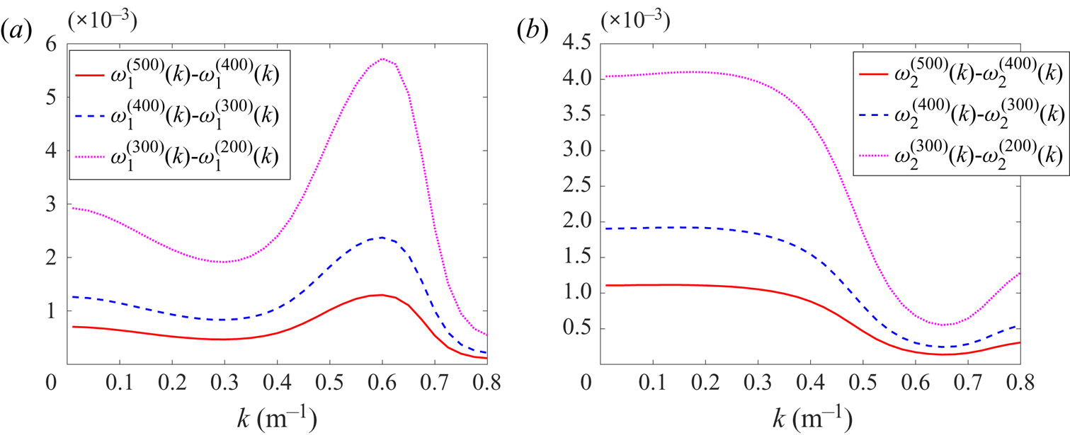
 $n=2$, as shown in figure 2. We can find that the difference of
 $\omega ^{(N)}_n(k)$ becomes smaller as
 $N$ increases for
 $n=1$ and
 $n=2$. In particular, it was shown that
 $(\omega _1^{(500)}(k)-\omega _1^{(400)}(k))$ is less than
 $10^{-3}\ \mathrm {s}^{-1}$, where
 $0<k<0.8$ m
 $^{-1}$. Below,
 $\omega _n(k)$ are approximated by
 $\omega _n^{(500)}(k)$ for elastic ice,
 $n=1,2,3,4,5$ and
 $0<k<k^\ast$. For each
 $k$,
 $n$ and correspondingly
 $\omega _n(k)$, the truncated system (3.20) with the matrix
 ${\boldsymbol{\mathsf{A}}}^\ast _N(k,\omega _n(k))$ is solved with respect to the vector
 $\boldsymbol {\hat {F}}_n^{(N)}(k)=(\hat {F}_{n,1}^{(N)}(k), \hat {F}_{n,2}^{(N)}(k),\ldots )^\textrm {T}$, which provides the wave profile across the channel using (3.1). To calculate the non-trivial solutions of the truncated system with zero determinant, we find an
 $i$th column of
 ${\boldsymbol{\mathsf{A}}}^\ast _N(k,\omega _n(k))$ with the largest
 $\sum _{j=1}^{N}({\boldsymbol{\mathsf{A}}}_N^\ast )_{ij}^2$, set
 $\hat {F}_i^{(N)}=1$ and move this column to the right-hand side of the system. Next we delete the
 $i$th row from the system to keep the resulting non-homogeneous system symmetric. Note that the obtained vector solution with
 $\hat {F}_i^{(N)}=1$ being multiplied by any constant is also a solution of the truncated system. A constant is selected for each
 $k$ and
 $n$ in such a way that the maximum magnitude of the
 $n$th wave elevation across the channel including the lead is equal to
 $1$. The wave amplitude is not determined in the present problem.
Convergence analysis of the roots  $\omega ^{(N)}_n(k)$ with respect to
 $N$ for
 $a=1.1\ \mathrm {m}$,
 $L=12\ \mathrm {m}$,
 $H=5\ \mathrm {m}$,
 $h=0.05\ \mathrm {m}$,
 $n=1$ (a) and
 $n=2$ (b).

For the model of rigid ice, see § 4, the system (4.16) is solved using the algorithm described above for elastic ice with the only difference that the truncation of the matrix in (4.16) with  $N=150$ provides the same accuracy of the results as
 $N=500$ in the model of elastic ice.
5.2. Validation of the algorithm
For a shrinking lead,  $a\to 0$, the present problem describes waves propagating in the frozen channel with the longitudinal crack at the centre of the ice cover. The latter problem was studied by Ren et al. (Reference Ren, Wu and Li2020) for the following conditions:
 $H=5\ \mathrm {m}$,
 $L=10\ \mathrm {m}$,
 $h=0.1\ \mathrm {m}$,
 $\rho _i=917\ \mathrm {kg}\ \mathrm {m}^{-3}$,
 $E=4.2\times 10^9\ \mathrm {N}\ \mathrm {m}^{-2}$,
 $\nu =0.3$,
 $\rho =1000\ \mathrm {kg}\ \mathrm {m}^{-3}$,
 $g=9.81\ \mathrm {m}\ \mathrm {s}^{-2}$. Dispersion relations for these conditions of symmetric waves with
 $n=1$ and
 $n=2$, which are obtained by the present algorithm with
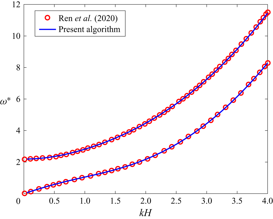
 $a=0$, are shown in figure 3 together with the dispersion relations for the same waves computed by Ren et al. (Reference Ren, Wu and Li2020), where
 $\omega ^*=\omega /\sqrt {g/H}$. It is seen that the results are in a very good agreement.
Dispersion relations for the first two symmetric hydroelastic waves by Ren et al. (Reference Ren, Wu and Li2020) (circle markers) and by the present algorithm (solid lines).

6. Numerical results
The results of the present study are presented in terms of dispersion relations, phase and critical speeds, profiles and strains of the symmetric waves propagating along the channel with a lead. Numerical calculations are performed for a freshwater ice with density  $\rho _i=917\ \mathrm {kg}\ \mathrm {m}^{-3}$, Young's modulus
 $E=4.2\times 10^9\ \mathrm {N}\ \mathrm {m}^{-2}$ and Poisson's ratio
 $\nu =0.3$. The thickness
 $h$ of the ice sheet is varied from
 $0.5\ \mathrm {mm}$ to
 $2\ \mathrm {m}$. The half-width
 $L$ of the channel is
 $12\ \mathrm {m}$ and the water depth
 $H$ is
 $5\ \mathrm {m}$. The half-width
 $a$ of the lead is varied from
 $0\ \mathrm {m}$ (a crack) to
 $6\ \mathrm {m}$. Water density is
 $\rho =1000\ \mathrm {kg}\ \mathrm {m}^{-3}$ and the gravity acceleration is
 $g=9.8\ \mathrm {m}\ \mathrm {s}^{-2}$. Dimensions of the channel,
 $L$ and
 $H$, and the ice characteristics,
 $\rho _i$,
 $E$ and
 $\nu$ are constant in this analysis. Dimensionless variables and parameters are used below. They are denoted by an asterisk,
 $k^*=kH$,
 $\omega ^*=\omega /\sqrt {g/H}$,
 $h^*=h/H$,
 $a^*=a/H$,
 $L^*=L/H$,
 $c^*=c/\sqrt {gH}$,
 $\lambda ^*=\lambda /H$,
 $\varPhi ^*=\varPhi /H^2$.
6.1. Dispersion relations
The dispersion relations,  $\omega ^*=\omega ^*_n(k^*)$, of hydroelastic waves in an ice channel with a lead are expected to converge to the corresponding dispersion relations of waves in the same channel without ice,
 $\omega _n^{*(f)}(k^*)$, which are defined in § 3, as the ice thickness decreases, and to the dispersion relations of waves in the same channel with rigid ice,
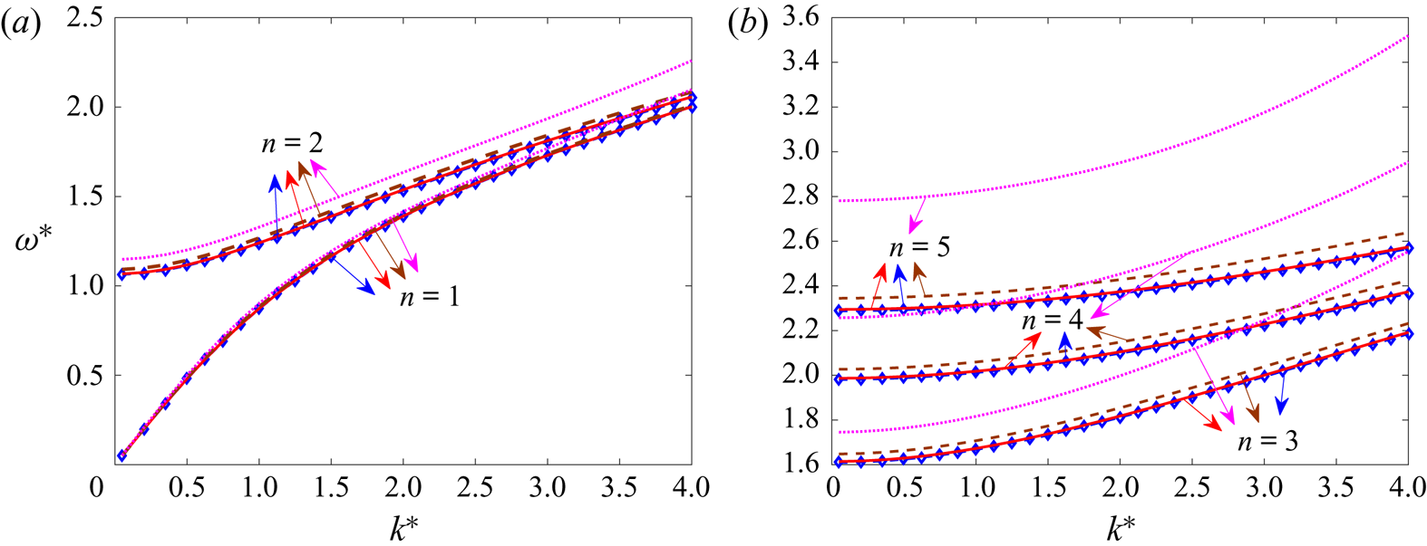
 $\omega _n^{*(r)}(k^*)$, which are defined in § 4, as the ice thickness increases. Figure 4 shows dispersion relations of waves with
 $n=1,2,3,4,5$ for
 $h^*=4\times 10^{-3},\ 1\times 10^{-3},\ 1\times 10^{-4}$ and for the same channel without ice. The half-width of the lead is
 $a^*=0.22$ in this figure. It is seen that the wave frequencies
 $\omega ^*_n(k^*)$ increase with increasing ice thickness for given
 $n$ and
 $k^*$. Higher wave frequencies are more sensitive to the ice thickness than the low frequencies with
 $n=1$ and
 $2$; see figure 4(b). The dispersion relations of hydroelastic waves for
 $h^*=1\times 10^{-4}$ are close to the corresponding dispersion relations without ice; see figure 4(a,b). The relative differences between the corresponding frequencies,
 $|\omega ^*_n(k^*)-\omega _n^{*(f)}(k^*)|/\omega ^*_n(k^*)$, where
 $\omega ^*_n(k^*)$ are for
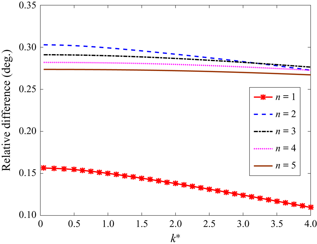
 $h^*=1\times 10^{-4}$, are shown in figure 5. It is seen that the relative differences for
 $n\leq 5$ are small. The corresponding wave profiles are different near the walls of the channel, see figure 15, where the amplitudes of the hydroelastic waves are zero because of the ice clamped conditions on the vertical walls. Figure 5 shows that the relative differences decay with
 $k^*$. However, the absolute differences increase with
 $k^*$, which corresponds to our expectation that a small ice thickness is still important for relatively short waves.
Dispersion relations for hydroelastic waves in the ice channel with the lead of half-width  $a^*=0.22$ and ice thickness
 $h^*=1\times 10^{-4}$ (solid lines),
 $1\times 10^{-3}$ (dashed lines) and
 $4\times 10^{-3}$ (dotted lines) for (a)
 $n=1$ and
 $n=2$, (b)
 $n=3,4,5$. Dispersion relations for the channel without ice cover are shown by rhombus markers.

Relative differences between the frequencies  $\omega ^*_n(k^*)$ of hydroelastic waves for
 $h^*=1\times 10^{-4}$,
 $a^*=0.22$ and the corresponding frequencies
 $\omega _n^{*(f)}(k)$ of the water waves in the same channel without ice for
 $n=1,2,3,4,5$.

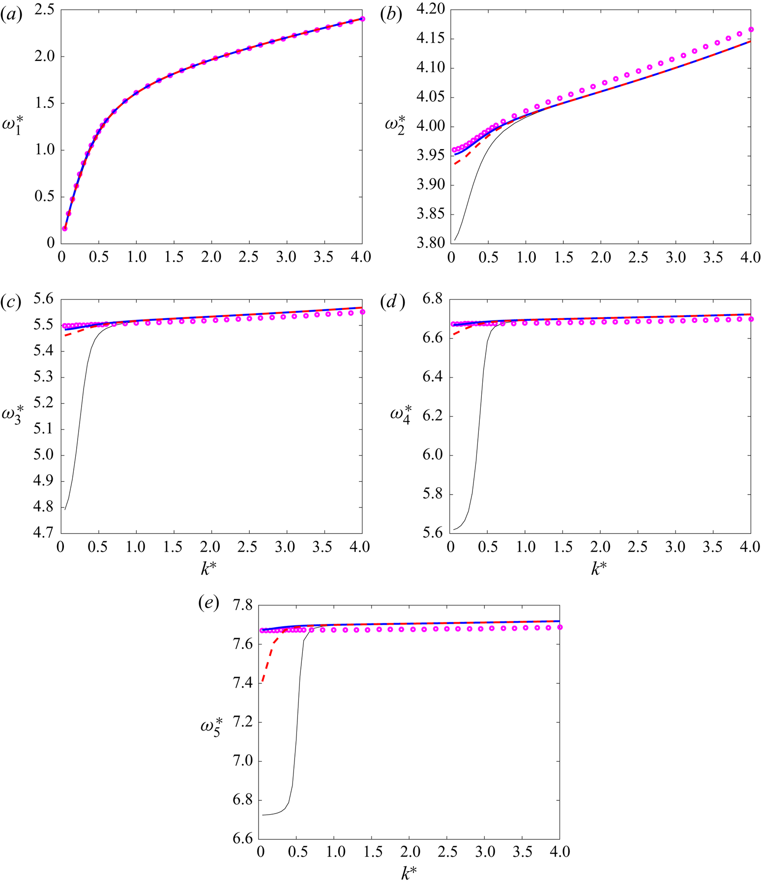
The frequencies of the hydroelastic waves  $\omega ^*_n(k^*)$, see § 3, are expected to converge to the wave frequencies calculated by the rigid ice model, see § 4, where the ice thickness increases. The dispersion relations of hydroelastic waves are shown in figure 6(a–e) for
 $n=1,2,3,4,5$ and an ice thickness of
 $h^*=0.2$,
 $0.3$ and
 $0.4$. The frequencies of waves propagating in the channel with rigid ice plates are also shown there. The half-width of the lead is
 $a^*=0.22$ in figure 6. Note different ranges for the frequencies
 $\omega ^*_n(k^*)$. The first frequency,
 $\omega ^*_1(k^*)$, is weakly dependent on the ice thickness and is well approximated by the rigid ice model, see figure 6(a),
 $\omega ^*_1(k^*) \approx \omega _1^{*(r)}(k^*)$, where
 $h^* \geq 0.2$. The frequencies
 $\omega ^*_n(k^*)$ calculated with
 $h^*=0.2$,
 $0.3$ and
 $0.4$ for
 $n=2,3,4,5$, see figure 6(b–e), are close to each other and to the corresponding frequencies
 $\omega _n^{*(r)}(k^*)$ by the rigid ice model for short waves, where
 $k^*>1$. For long waves,
 $0<k^*<1$, the ice thickness of
 $h^*=0.2$ is not large enough for the rigid ice model. However, the frequencies
 $\omega ^*_n(k^*)$ for
 $h^*=0.4$ are well approximated by
 $\omega _n^{*(r)}(k^*)$, where
 $n=2,3,4,5$. Hydroelastic waves in the ice cover can be modelled within the thin elastic plate approximation (2.1) if the ice thickness
 $h^*$ is much smaller than the wavelength
 $\lambda ^*=2 {\rm \pi}/k^*$, say
 $h^*/\lambda ^*\lt 0.1$. This inequality gives
 $k^*\lt {\rm \pi} /(5h^*)$ and
 $k^*<1.57$ for
 $h^*=0.4$. For shorter waves, the thin-plate approximation is not applicable but then the ice cover can be modelled as a rigid plate; see figure 6.
Dispersion relations for the first five hydroelastic waves,  $\omega ^*=\omega ^*_n(k^*)$, and ice thickness
 $h^*=0.2$ (thin solid lines),
 $h^*=0.3$ (dashed lines) and
 $h^*=0.4$ (thick solid lines). The corresponding frequencies by the rigid ice model are shown by circle markers.

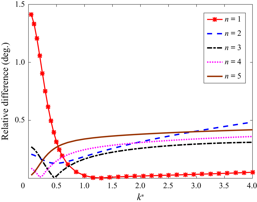
The relative differences between the corresponding frequencies  $|\omega ^*_n(k^*)-\omega _n^{*(r)}(k^*)|/ \omega ^*_n(k^*)$, where
 $\omega ^*_n(k^*)$ are calculated for
 $h^*=0.4$, are shown in figure 7 for
 $n=1,2,3,4,5$. Only for long waves with
 $k^*<0.25$, the relative difference for the lowest frequency
 $\omega ^*_1(k^*)$ is greater than
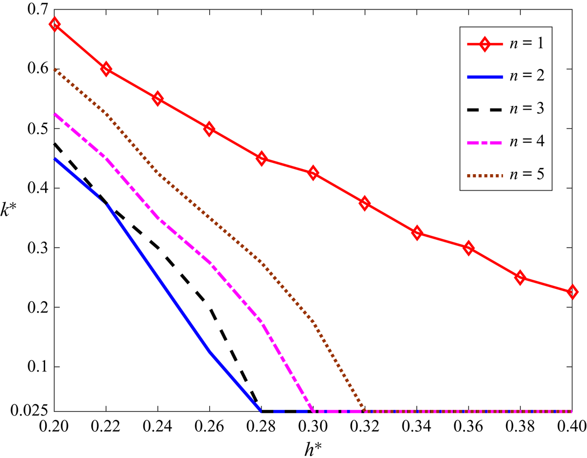
 $1\,\%$. Therefore, it is reasonable to conclude that the ice elasticity is less important for short waves and thick ice. This is illustrated by figure 8, where the
 $k^*$-
 $h^*$ plane (wavenumber
 $k^*$ and ice thickness
 $h^*$),
 $0.2<h^*<0.4$, is divided for each mode
 $\omega ^*_n(k^*)$ by a corresponding line into two parts. The relative difference for
 $\omega ^*_n(k^*)$ is less than
 $1\,\%$ above the corresponding line, see the legend in figure 8, where the ice elasticity can be neglected. The figure shows that the ice cover can be approximated as rigid for the first five modes if the wave is short enough,
 $k^*>b^*-d^*\cdot h^*$, where
 $b^*=1.2$,
 $d^*=2.5$ and
 $0.2<h^*<0.4$.
Relative differences between the frequencies  $\omega ^*_n(k^*)$ of hydroelastic waves for
 $h^*=0.4$ and the corresponding frequencies
 $\omega _n^{*(r)}(k^*)$ of water waves in the same channel with the lead
 $a^*=0.22$ and rigid ice cover for
 $n=1,2,3,4,5$.

The  $k^*$-
 $h^*$ plane with the regions, where ice elasticity can be neglected for waves with numbers
 $n=1,2,3,4,5$ with a relative difference less than
 $1\,\%$ in terms of the corresponding dispersion relation.

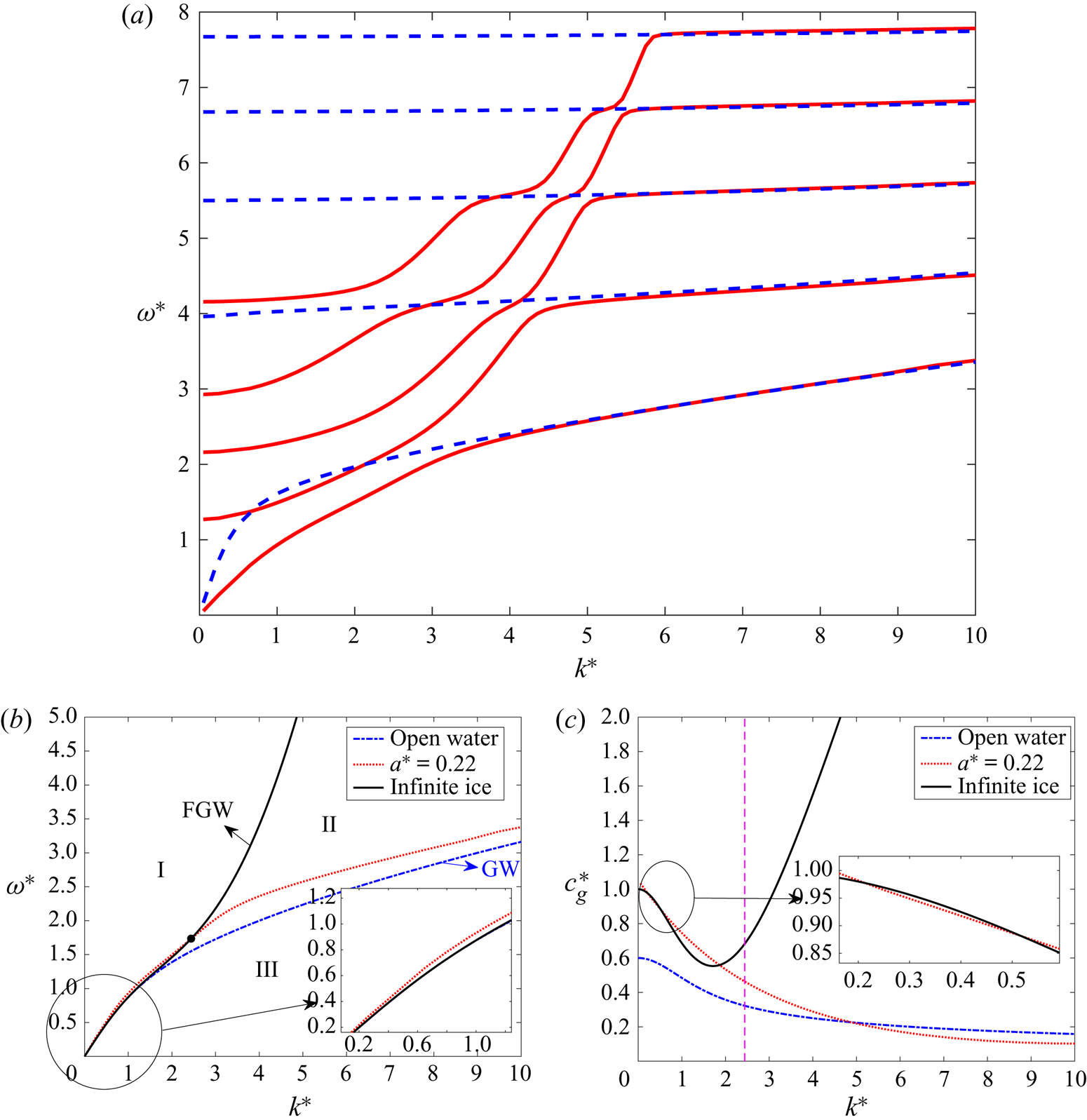
The dispersion relations of the first five hydroelastic waves are shown in figure 9(a) for ice thickness  $h^*=0.01$ in both elastic and rigid ice models. It is seen that the ice flexibility is important for long waves,
 $k^*<6$. For short waves with
 $k^*>6$, the ice cover with thickness
 $h^*=0.01$ behaves as a rigid plate. Figure 9(b) shows the dispersion relations for waves propagating in the open water and in an infinite ice sheet together with the dispersion relation of the first hydroelastic wave for the ice thickness
 $h^*=0.01$ and the dimensionless width of the lead
 $a^*=0.22$. The dispersion relations of flexural-gravity waves and gravity waves divide the quarter plane ,
 $k^*>0$ and
 $\omega ^*>0$, into three regions I, II and III. We can see that the dispersion curve of the first hydroelastic wave starts in the region I at
 $k^*=0$ and
 $\omega ^*=0$, where
 $\omega ^*>\omega ^*_{FGW}$ (here FGW denotes flexural-gravity waves), intersects the flexural-gravity wave curve at
 $k^*=2.44$ and
 $\omega ^*=1.73$ which is shown by the black point in figure 9(b), and then stays in region II as predicted by Marchenko (Reference Marchenko1997). The first hydroelastic wave, the dispersion relation of which is shown by the dotted line in figure 9(b), is strongly dependent on both the width of the channel and the width of the lead. However, in terms of interpretation of regions I and II, the hydroelastic wave with a frequency
 $\omega ^*(k^*)$ in region I, where
 $k^*<2.44$, can be considered as the flexural-gravity wave propagating in the ice cover with the dimensionless wavenumber
 $k^*$ in the
 $x$-direction along the channel and the dimensionless wavenumber
 $k^*_y$ in the
 $y$-direction across the channel, where
 $\omega ^*(k^*)=\omega ^*_{FGW}(K^*)$ and
 $K^*=\sqrt {(k^*)^2+(k_y^*)^2}$. This flexural-gravity wave in the ice plate has the same dimensionless wavenumber
 $k^*$ in the
 $x$-direction, as the hydroelastic wave in the channel with the lead, and the real dimensionless wavenumber
 $k_y^*$ in the
 $y$-direction. This flexural-gravity wave propagates in the
 $x$-direction, which is along the channel, and in the
 $y$-direction, which is across the channel. Therefore, we can conclude that the long hydroelastic waves in region I can be detected far from the ice plate edge inside the ice sheet. The same arguments applied to region II provides that
 $k_y^*$ is imaginary here, which means that such short waves do not penetrate deep in the ice sheet. The hydroelastic waves in region II decay exponentially in the ice cover with the distance from the ice edge. Figure 9(b) shows that shorter waves decay quicker with the distance. As to the comparison of our hydroelastic wave with gravity waves in both regions I and II, see figure 9(b), the hydroelastic wave can travel both along the channel with the wavenumber
 $k^*$ and across the lead with the real wavenumber
 $k_y^*$. The waves from region II, where
 $k^*>2.44$, are localised in the lead.
(a) Dispersion relations for the first five waves,  $n=1,2,3,4,5$,
 $a^*=0.22$, calculated within the elastic ice model with an ice thickness of
 $h^*=0.01$ (solid lines) and within the rigid ice model (dashed lines). (b) Dispersion relations for waves propagating in open water, infinite ice sheet and for the first hydroelastic wave in an ice channel with
 $a^*=0.22$. (c) Group speeds for waves propagating in open water, infinite ice sheet and for the first hydroelastic wave in an ice channel with
 $a^*=0.22$.

The dispersion relation of the hydroelastic wave in the channel with the lead (dotted line in figure 9b) and the dispersion relation of the flexural-gravity waves shown by the solid line intersect each other at  $k^*=2.44$; see the black point in figure 9(b). At this point, the wavelength, wave frequency and the phase speed of the flexural-gravity waves in the ice and of the first hydroelastic wave in the channel with the lead are equal. However, their group speeds are not equal to each other; see figure 9(c). The group speed of the hydroelastic waves in the channel is slightly higher than the group speed of the flexural-gravity waves in the ice sheet for
 $k^*<0.21$ and
 $0.52<k^*<1.86$ and smaller for
 $0.21<k^*<0.52$ and
 $k^*>1.86$. The intervals might be affected by accuracy of the numerical calculations of the parameters of the hydroelastic wave. An asymptotic solution of the present problem with a lead as
 $k^*\to 0$ would be helpful to clarify the difference of the long hydroelastic wave from the flexural-gravity wave. Marchenko (Reference Marchenko1999) showed that a similar situation occurs for linear hydroelastic waves propagating in a semi-infinite ice sheet attached to a vertical wall. In the latter problem, the wave profile is given analytically, which makes it possible to investigate the effect of the vertical wall on the propagating hydroelastic waves in more details. The dispersion relation of the hydroelastic wave in the semi-infinite ice sheet attached to a vertical wall also intersects the dispersion relation of the flexural-gravity waves in the infinite ice sheet at a single point, where the wavelength, wave frequency and both the phase and group speeds of the hydroelastic waves in infinite and semi-infinite ice sheets are equal; see Marchenko (Reference Marchenko1999). This comparison shows that the presence of a lead in the ice channel is important for characteristics of the hydroelastic waves in the channel.
A gravity wave from the lead cannot enter the ice sheet if  $k_y^*$ is much smaller than
 $k^*$, which implies that the angle between the wave propagation and the normal to the ice edge is large. The corresponding analysis has not been done yet. This analysis is expected to provide the conditions, where the ice strains in the hydroelastic waves are relatively large.
6.2. Phase speeds and critical speeds of hydroelastic waves in the ice channel
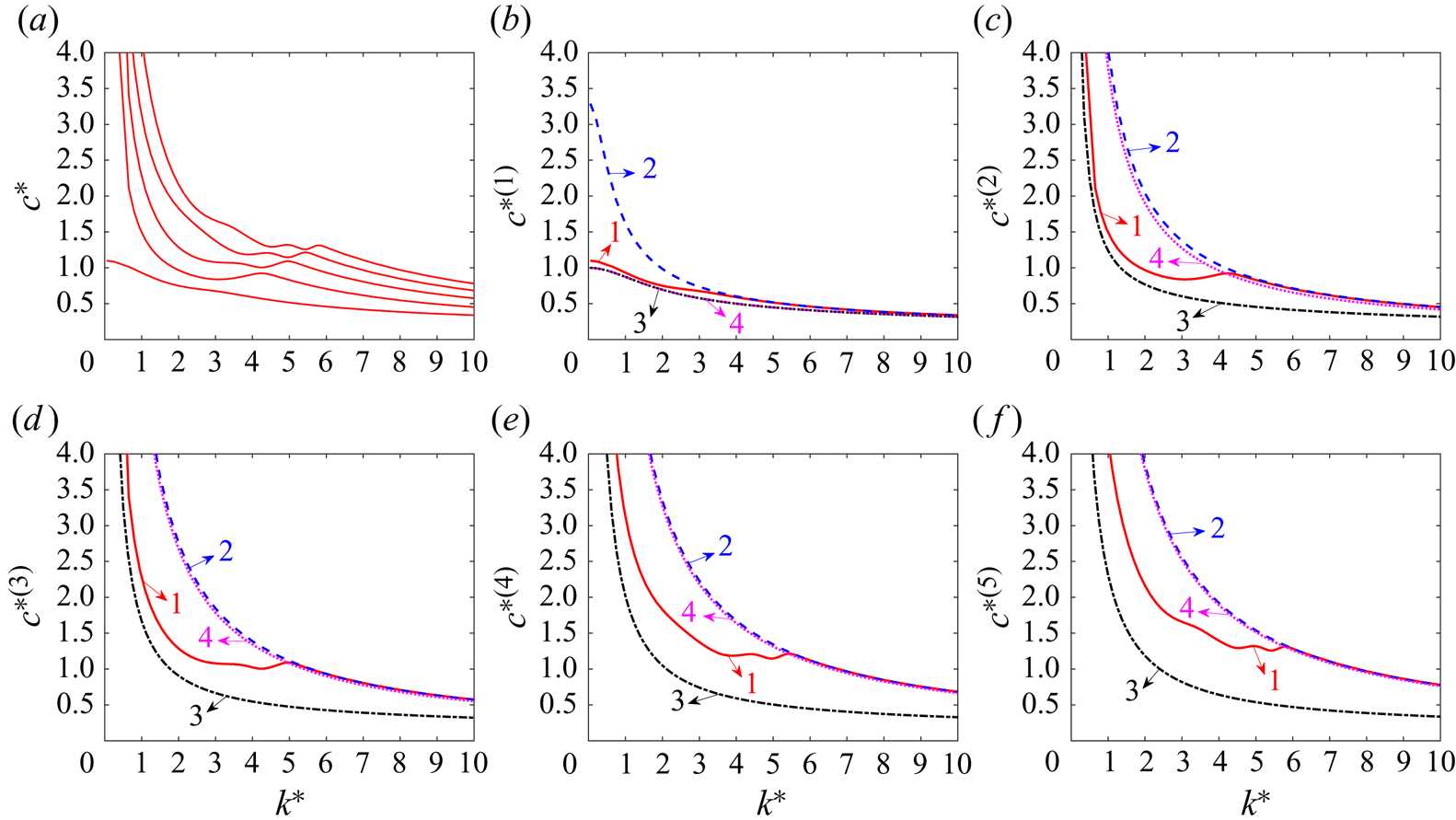
The phase speeds,  $c^{*(n)}(k^*)=\omega ^*_n(k^*)/k^*$, of the first five hydroelastic waves in the ice channel with the lead,
 $a^*=0.22$, are shown in figure 10(a) for the ice thickness
 $h^*=0.01$. The presence of the lead significantly changes the behaviour of the phase speeds. The phase speeds in the ice channel without a lead decrease with an increase of
 $k^*$ for small
 $k^*$, then take their minimum values, which are known as critical speeds, and then increase with an increase of
 $k^*$ again; see Korobkin et al. (Reference Korobkin, Khabakhpasheva and Papin2014, figure 6(b)). A vessel moving along an ice channel at a critical speed generates ice deflections, which cannot be described within the linear wave theory; see Marchenko (Reference Marchenko1997). For a weakly nonlinear regime and two-dimensional problems, Parau & Dias (Reference Parau and Dias2002) derived a forced nonlinear Schrodinger equation for the envelope of ice sheet deflections caused by a load moving at a critical speed. Dinvay, Kalisch & Parau (Reference Dinvay, Kalisch and Parau2019) developed a fully dispersive weakly nonlinear model describing flexural-gravity waves in a floating elastic plate, excited by a moving load. For larger amplitudes, both forced and free steady waves were computed by Guyenne & Parau (Reference Guyenne and Parau2012) using direct numerical simulations with a boundary integral method.
Phase speeds of hydroelastic waves with  $n=1,2,3,4,5$ as functions of the wavenumber. (a) Phase speeds for ice thickness
 $h^*=0.01$, where
 $c^{*(n+1)}(k^*)>c^{*(n)}(k^*)$ for
 $n \geq 1$ and
 $k^* \geq 0$. (b–f) Phase speeds
 $c^{*(n)}(k^*)$ of the hydroelastic waves for
 $h^*=0.01$ (solid lines, 1), waves within the rigid ice model (dashed lines, 2), waves in the channel without ice (dashed–dotted lines, 3) and waves in the channel without ice with the reduced width
 $2a^*$ (dotted lines, 4).

The presence of water in the channel is negligible for relatively short waves  $k^*>5$ for
 $h^*=0.01$; see Shishmarev, Khabakhpasheva & Korobkin (Reference Shishmarev, Khabakhpasheva and Korobkin2016, figure 15(a)). Such waves are elastic but not hydroelastic. The presence of a lead makes the short waves propagate mainly along the lead as water waves with the ice on the sides of the lead much less involved in the wave motion. As a result, each wave mode for a channel with a lead, except for the first mode, has at least two critical speeds, see figure 10(a), where
 $\mathrm {d}c^{*(n)}/\mathrm {d}k^*=0$ and the phase speed is equal to the group speed,
 $c^{*(n)}_g(k^*)=\mathrm {d}\omega ^*_n/\mathrm {d}k^*$. At each corresponding wavenumber, we have
 $\mathrm {d}^2\omega ^*_n/\mathrm {d}k^{*2}=k^*\, \mathrm {d}^2 c^{*(n)}/\mathrm {d}k^{*2}$, which is positive if the phase speed is minimum at that
 $k^*$ and negative if the phase speed is maximum at that
 $k^*$. Note that
 $\frac {1}{2}(\omega ^{*}_n(k^*))''$ is the coefficient of the dispersion term in the nonlinear Schrodinger equation describing the weakly nonlinear wave propagating at the critical speed; see Guyenne & Parau (Reference Guyenne and Parau2012). Dispersion relations with several critical speeds for a wave mode appear, for example, also in the problem of internal waves under ice ; see Wang et al. (Reference Wang, Parau, Milewski and Vanden-Broeck2014, figure 2(b)) for the internal (slow) wave mode.
Analysis of the phase speeds is presented in figure 10(b–f). Figure 10(b) shows the phase speed of the hydroelastic wave with the lowest frequency  $\omega ^*_1(k^*)$; see line 1. This phase speed decreases monotonically with an increase of the wavenumber. Therefore,
 $\mathrm {d}c^{*(1)}/\mathrm {d}k^*<0$ for
 $k^*>0$ and
 $\mathrm {d}c^{*(1)}/\mathrm {d}k^*=0$ only at
 $k^*=0$. The critical speed of this hydroelastic wave,
 $c^{*(1)}(0)$, is equal to
 $1.1$, which is slightly higher than the corresponding critical speed of long water waves in the same channel but without ice,
 $c^{*(1)}_f(0)=1$; see line 3. Curve 4 is also for water waves but in the channel of reduced width equal to the width of the lead
 $2a^*$. Figure 10(b) shows that curve 3 and curve 4 are identical, because the first phase speed of waves in the channel without ice,
 $c^{*(1)}_f(k^*)=\omega ^{*(f)}_1(k^*)/k^*=\sqrt {\tanh (k^*)/k^*}$, depends only on the non-dimensional wavenumber
 $k^*$ but not on the channel width. The phase speed by curve 2 is for the same channel and the lead but within the rigid ice model. Figure 10(b) shows that the phase speed of the first hydroelastic wave can be roughly approximated by the phase speed of the one-dimensional water wave. The rigid ice model predicts much greater phase speed for long waves,
 $k^*<3.5$, where the flow between the lead region,
 $|y^*|<a^*$, and the region under the rigid ice,
 $a^*\lt |y^*|\lt L^*$, is significant. For a shorter wave, the flow between these regions is weak and all four phase speeds are close to each other.
For higher wave modes,  $n=2,3,4,5$ in figure 10(c–f), the presence of ice plates of thickness
 $h^*=0.01$ in the channel is important, which can be concluded by comparing the phase speeds presented by curves
 $1$ and
 $3$. Curves
 $1,2$ and
 $4$ are very close to each other for
 $k^*>5$, see figure 10(c–f), which shows that the computed waves are gravity waves confined to the lead region. However, the fluid under the ice sheets is not at rest even for the rigid ice model. From (4.6) and (4.11), we find that
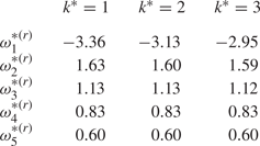
 \begin{equation} \dfrac{\partial \varPhi}{\partial y}(a^*,z^*)=\sum_{m=0}^{\infty}\dfrac{-\cosh[({\unicode{x00E6}}_mH)(z^*+1)](\lambda_mH)}{({\unicode{x00E6}}_mH)\sinh({\unicode{x00E6}}_m H)}\sin((\lambda_mH) a^*)\sum_{k=0}^{\infty}F_k S_{km}, \end{equation}
at the ice edge,  $y^*=a^*$ for the rigid ice model. The dimensionless numerical values of
 $({\partial \varPhi ^*}/{\partial y^*})(a^*,z^*)$ at
 $z^*=0$ for
 $k^*=1,2,3$ are shown in table 1. We can find that the values
 $({\partial \varPhi ^*}/{\partial y^*})(a^*,0)$ are not equal to zero for different wave modes and wavenumbers, which indicates that the rigid ice model is not equivalent to the channel without ice with the reduced width
 $2a^*$. However, it should be noted that the absolute values of
 $({\partial \varPhi ^*}/{\partial y^*})(a^*,0)$ decrease with the wavenumber increase. The most notable feature of long waves in figure 10(c–f) is the presence of several critical speeds for each mode. We count two critical speeds for
 $n=2,3$ and four critical speeds for
 $n=4,5$.
The dimensionless velocity of the flow across the channel,  $({\partial \varPhi ^*}/{\partial y^*})(a^*,z^*)$, at the ice edge,
 $z^*=0$, for different wavenumbers and different wave modes within the rigid ice model.

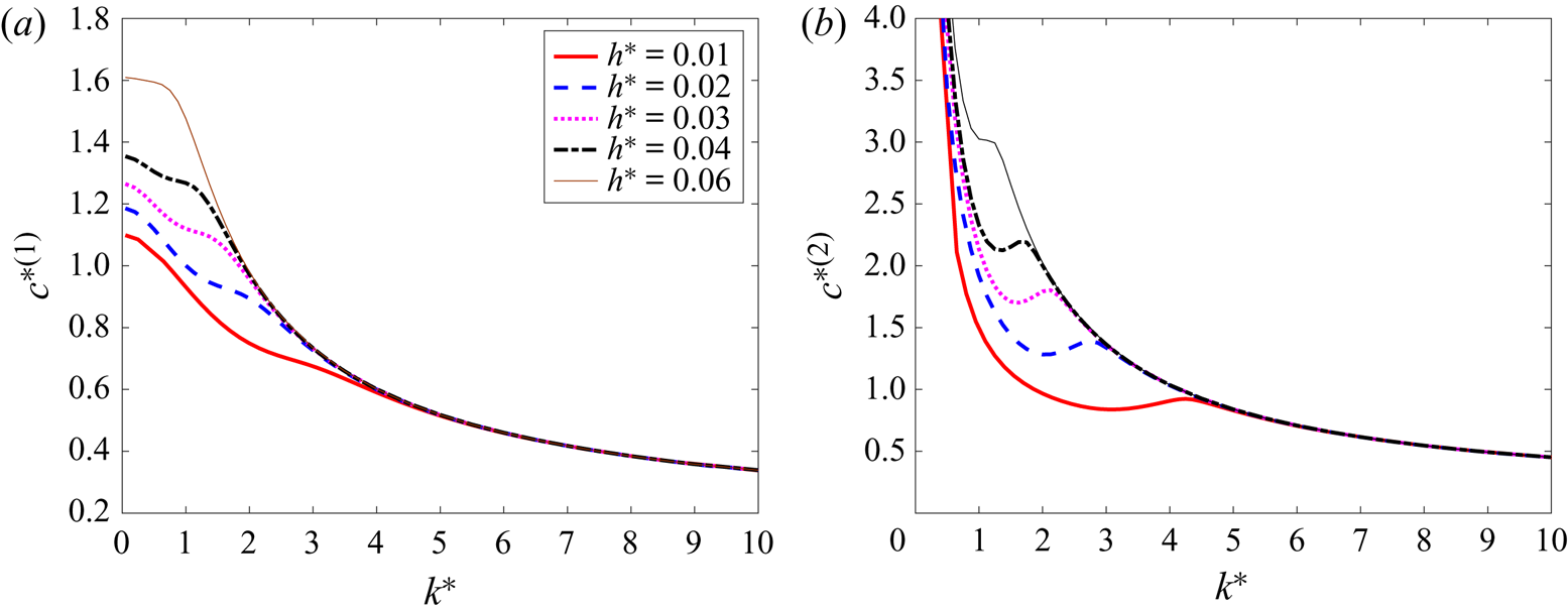
To investigate the influence of ice thickness on the phase speeds, the first and second phase speeds for different ice thicknesses are shown in figure 11. For a given wavenumber, we find that the phase speeds increase with an increase of the ice thickness for  $c^{*(1)}(k^*)$ and
 $c^{*(2)}(k^*)$. We observe from figure 11(a) that there is no point with
 $\mathrm {d}c^{*(1)}/\mathrm {d}k^*=0$ for
 $k^*>0$. We also observe from figure 11(b) that there are two points with
 $\mathrm {d}c^{*(2)}/\mathrm {d}k^*=0$ for
 $h^*=0.01$,
 $h^*=0.02$,
 $h^*=0.03$ and
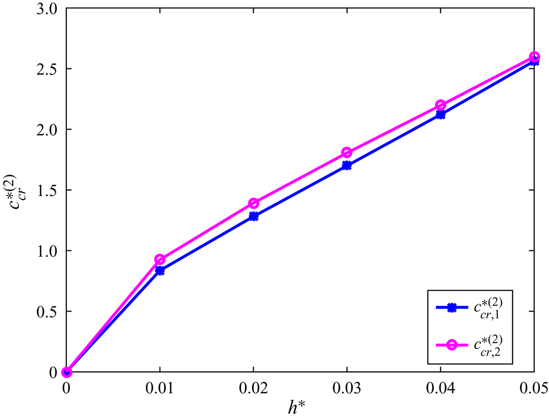
 $h^*=0.04$. The critical speeds increase with an increase of the ice thickness. However, for an ice thickness of
 $h^*=0.06$, there are no critical speeds for the second hydroelastic wave. The critical speeds of the second hydroelastic wave,
 $c^{*(2)}_{cr, 1}$ and
 $c^{*(2)}_{cr, 2}$, as functions of the ice thickness
 $h^*$ for the ice channel with the lead half-width
 $a^*=0.22$ are shown in figure 12. The first critical speed of the second hydroelastic wave,
 $c_{cr,1}^{*(2)}$ is always smaller than the second critical speed,
 $c^{*(2)}_{cr, 2}$; see also figure 11(b).
Phase speeds  $c^{*(n)}(k^*)$ for (a)
 $n=1$ and (b)
 $n=2$ as functions of the wavenumber for ice thickness
 $h^*=0.01$ (thick solid lines),
 $0.02$ (dashed lines),
 $0.03$ (dotted lines),
 $0.04$ (dashed-dotted lines) and
 $0.06$ (thin solid lines).

Critical speeds of the second hydroelastic wave,  $c^{*(2)}_{cr, 1}$ (lines with asterisk markers) and
 $c^{*(2)}_{cr, 2}$ (lines with circle markers), as functions of the ice thickness for
 $a^*=0.22$.

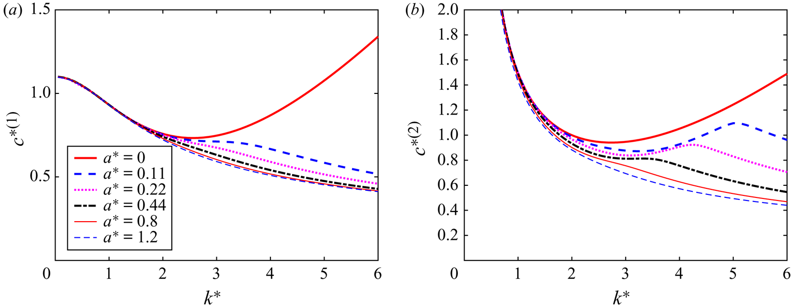
As to the influence of the width of the open water lead on the phase speeds, figure 13 shows the phase speeds of the first and second hydroelastic waves for  $h^*=0.01$ and different half-widths of the open water lead. It is seen that there is one critical speed for each wave without the lead of open water,
 $a^*=0$. However, for
 $a^*=0.11$,
 $0.22$,
 $0.44$,
 $0.8$ and
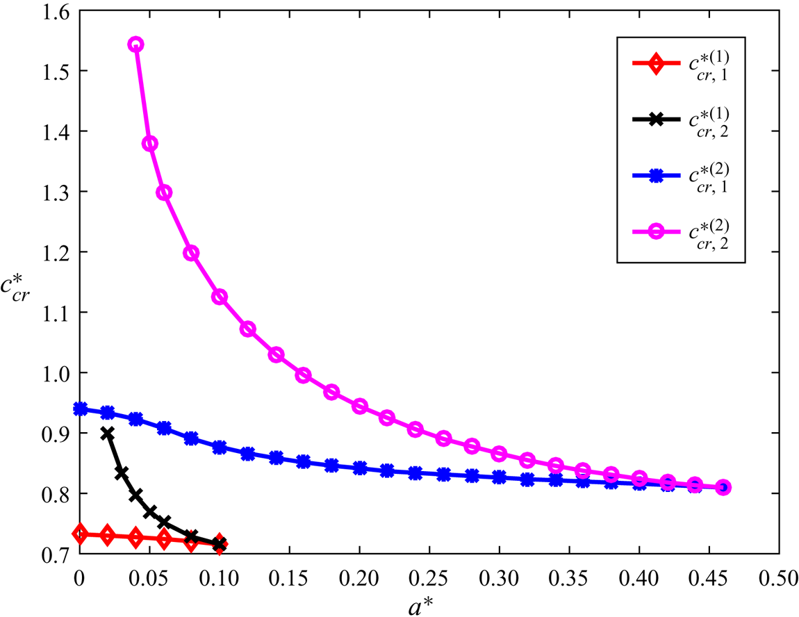
 $1.2$, there are no critical speed for the first hydroelastic wave, and two critical speeds for the second hydroelastic wave. It is worth further investigating the effect of the width of the open water lead on critical speeds. Figure 14 shows the critical speeds as functions of the half-width of the open water lead
 $a^*$ for the first and second hydroelastic waves with an ice thickness of
 $h^*=0.01$. Note that we do not count here the critical speed of the long first wave at
 $k^*=0$, which exists for any
 $a^*$. It is seen that there is no critical speed for the first hydroelastic wave with
 $a^*>0.1$. For
 $0.02 \leq a^* < 0.1$, there are two critical speeds for the first hydroelastic wave. For the second hydroelastic wave, there is one critical speed for
 $0<a^*<0.04$, there are two critical speeds for
 $0.04 \leq a^* < 0.46$, then the critical speeds merge at
 $a^*\approx 0.46$ and there are no critical speeds for
 $a^*>0.46$. The critical speeds decrease with an increase of the width of the lead.
Phase speeds  $c^{*(n)}(k^*)$ for (a)
 $n=1$, (b)
 $n=2$ and ice thickness
 $h^*=0.01$ as functions of the wavenumber without the lead (
 $a^*=0$, thick solid lines), and with the lead of half-width
 $a^*=0.11$ (thick dashed lines),
 $a^*=0.22$ (dotted lines),
 $a^*=0.44$ (dashed–dotted lines),
 $a^*=0.8$ (thin solid lines) and
 $a^*=1.2$ (thin dashed lines).

Critical speeds of the first and second hydroelastic waves as functions of the lead half-width  $a^*$ for ice thickness
 $h^*=0.01$.

6.3. Profiles of hydroelastic waves
Linear hydroelastic waves propagating in an ice channel with a lead are sinusoidal along the channel, see (2.6a,b), with the wavelength  $2{\rm \pi} /k^*$. For example, a wave with
 $k^*=0.5$ is of length
 $\lambda ^*=12.6$, which is greater than the channel width,
 $2L^*=4.8$, the channel depth,
 $H^*=1$, and the width of the symmetric lead,
 $2a^*=0.44$, in the main part of our calculations. The profiles of the waves across the channel are more complicated. The profile of the
 $n$th hydroelastic wave is described by the even function
 $F_n^*(y^*)$, where
 $|y^*|\lt L^*$, which is calculated as part of the solution. The functions
 $F_n^*(y^*)$ are normalised in such a way that their maximum magnitudes are equal to 1. The wave profiles
 $F_n^*(y^*)$ depend on the parameters of the channel and the ice plates, as well as on the wavenumber
 $k^*$. Only waves symmetric with respect to the centreline of the channel are considered in this study.
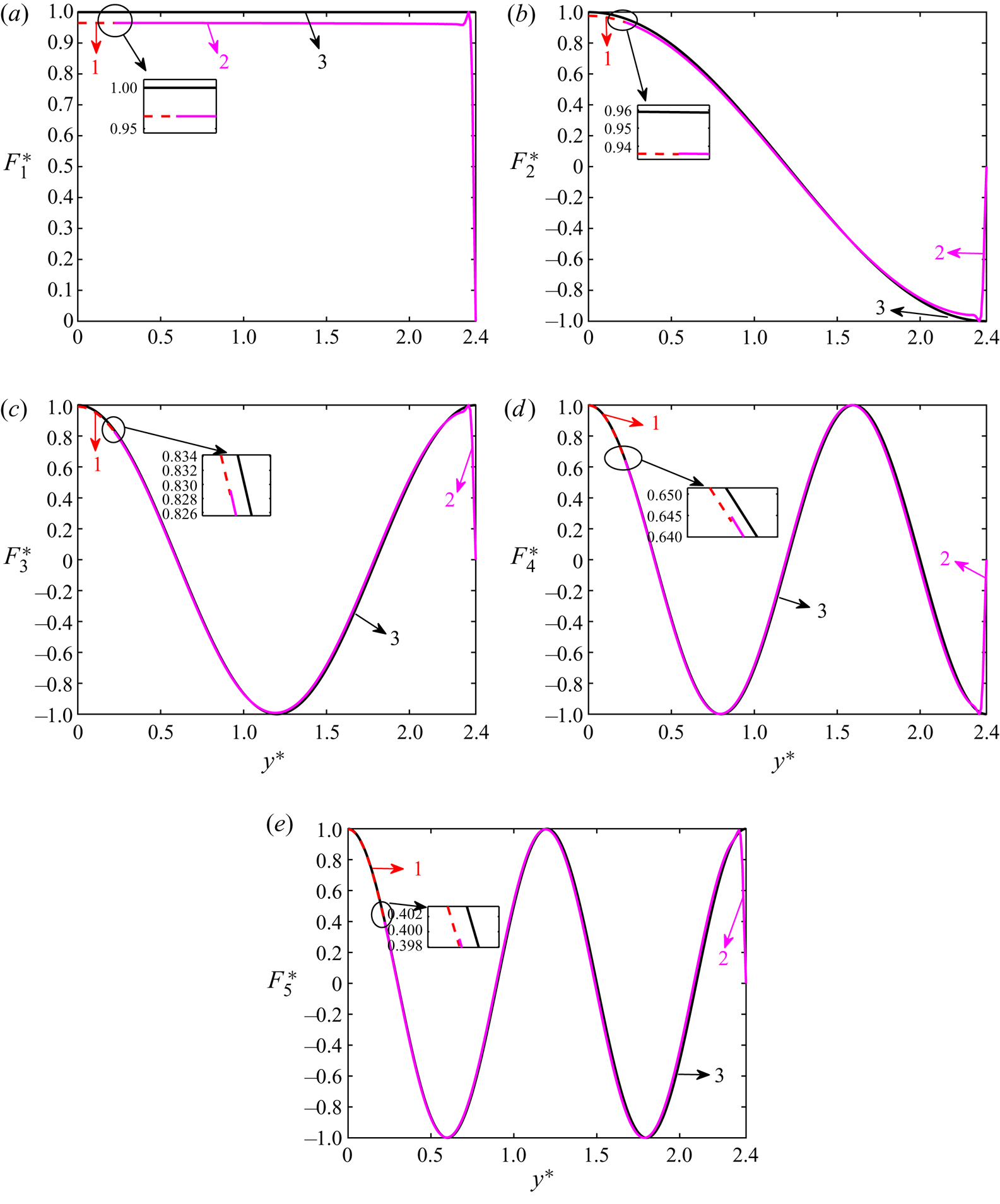
The computed profiles  $F_n^*(y^*)$ of the hydroelastic waves across the channel are shown in figure 15 for
 $n=1,2,3,4,5$ and a small ice thickness of
 $h^*=1\times 10^{-4}$. The half-width of the open water lead is
 $a^*=0.22$ and
 $k^*=0.5$. The wave profiles for the same channel without ice,
 $F_{n}^{*(f)}(y^*)=\cos (({(n-1){\rm \pi} }/{L^*})y^*)$, are also presented for comparison. Only half,
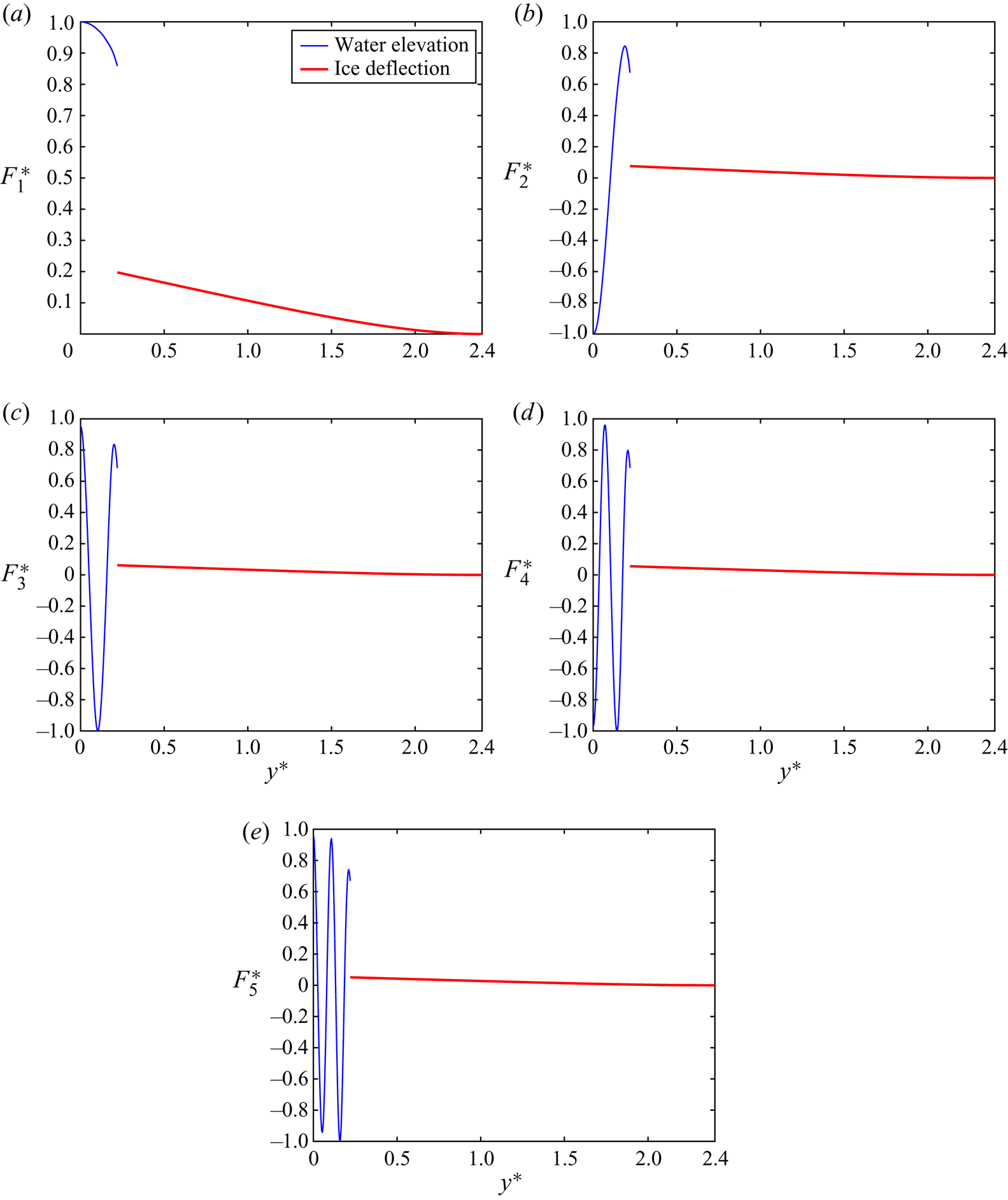
 $0\lt y^*\lt L^*$, of the channel width is shown because of the symmetry of the computed waves. One can see that the deflection of ice and elevation of the open water are close to each other at the ice edge,
 $y^*=a^*$, for
 $n=1,2,3,4$ and
 $5$, but not equal even for this small thickness of the ice. The wave profiles for the ice channel and the same channel without ice are close to each other except near the wall,
 $y^*=L^*$, where the ice plate is clamped to the wall,
 $F(L^*)=F'(L^*)=0$. Figure 15(a) shows that the lowest hydroelastic wave is of constant elevation inside the channel but changes significantly near the wall. This indicates high bending stresses near the wall for this wave.
Profiles  $F_n^*(y^*)$ of the hydroelastic waves (solid lines) for
 $k^*=0.5$ in the ice channel with a lead. Half-width of the lead
 $a^*=0.22$. Ice thickness is
 $h^*=1\times 10^{-4}$. The corresponding water wave profiles for the same channel without ice are shown by lines 3.

The hydroelastic wave profiles  $F_n^*(y^*)$ for
 $n=1,2,3,4$,
 $5$ and ice thickness
 $h^*=0.4$ are shown in figure 16. The computed deflections of the ice were multiplied by
 $100$ in this figure. It is seen that the ice deflection is very small compared with the water elevation in the lead.
Profiles  $F_n^*(y^*)$ of the hydroelastic waves for
 $k^*=0.5$ in the ice channel with a lead. Half-width of the lead
 $a^*=0.22$. Ice thickness is
 $h^*=0.4$. The deflections of ice were multiplied by
 $100$.

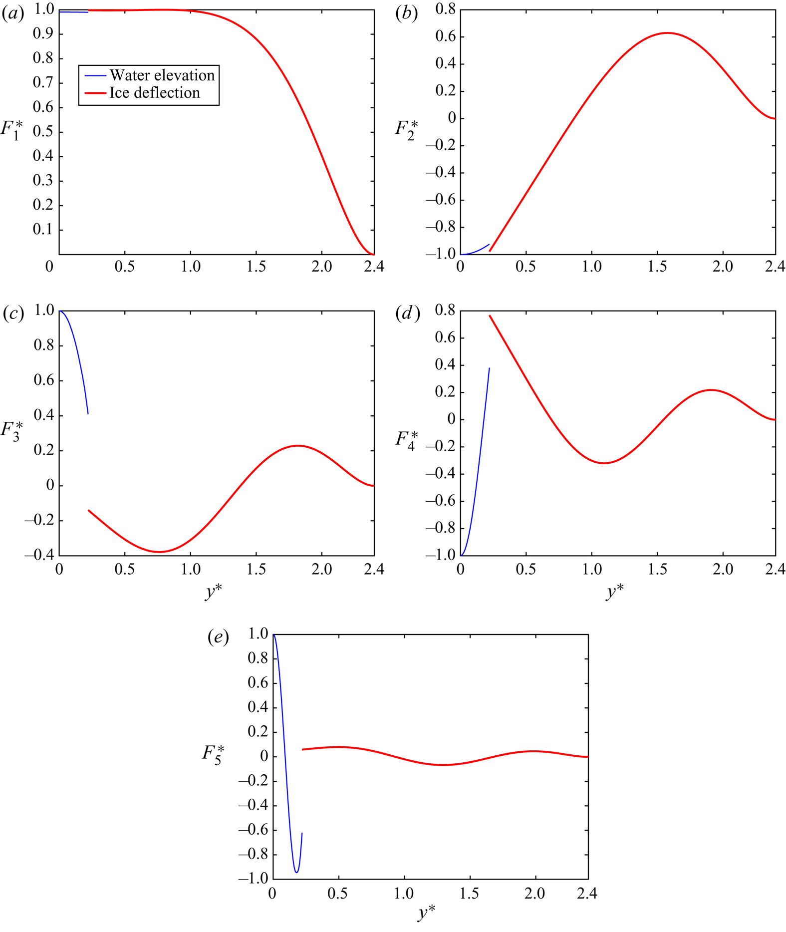
The wave profiles  $F_n^*(y^*)$ for
 $n=1,2,3,4,5$ and ice thickness
 $h^*=0.01$ are shown in figure 17. The functions
 $F_n^*(y^*)$ are defined by the series (3.1) with respect to the modes
 $\psi _m(y^*)$,
 $m\geq 1$, with the coefficients
 $F_{n,m}$ computed as explained in § 5.1. The non-dimensionalised modes are depicted in figure 21. Comparing figures 17 and 21, we can conclude that the main contribution to the
 $n$th wave profile
 $F_n^*(y^*)$ comes from the mode
 $\psi _m(y^*)$, where
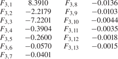
 $m \leq n$. In particular, the coefficients of the third wave profile,
 $F_{3,m}$, which are greater by module than
 $10^{-3}$ are shown in table 2. From the first equation of (2.6a,b) we can easily obtain the three-dimensional wave,
 $w_n^*=F_n^*(y^*) \cos (kx-\omega _n t)$, of waves propagating in the ice channel with a lead of open water. The three-dimensional wave profiles for
 $n=3$ and
 $t=0$ are also shown in figure 18. We can clearly see the difference between ice deformation and water elevation, as shown in figure 17(c). The wave changes periodically in the
 $x$-direction.
Profiles  $F_n^*(y^*)$ of the hydroelastic waves for
 $k^*=0.5$,
 $a^*=0.22$ and ice thickness
 $h^*=0.01$.

Three-dimensional wave for the third mode with  $a^*=0.22$ and ice thickness
 $h^*=0.01$.

The values of  $F_{3,m}$ greater than
 $10^{-3}$.

The strain distribution in the ice sheet is an important characteristic indicating potential breaking of ice caused by ship or wind generated waves. The maximum strain at each point of the ice surface can be obtained using the eigenvalues of the strain tensor,
 \begin{equation} \epsilon={\pm}\dfrac{h}{2} \left(\begin{array}{@{}cc@{}} w_{xx} & w_{xy}\\ w_{xy} & w_{yy}\end{array}\right) , \end{equation}
where  $h/2$ and
 $-h/2$ are for the lower and upper surface of the ice plate, respectively. To determine the maximum strain as a function of
 $y$ across the channel for each wave mode, we calculate four following functions of
 $y$ (Batyaev & Khabakhpasheva Reference Batyaev and Khabakhpasheva2015):
 \begin{align} \left.\begin{array}{c@{}} \displaystyle \epsilon_{max,1}(y)=\dfrac{h}{2} |F''(y)|, \quad \epsilon_{max,2}(y)=\dfrac{h}{2} k^2 |F(y)|,\\ \displaystyle \epsilon_{max,3}(y)=\dfrac{h}{2}kF'(y)\sqrt{\dfrac{4k^2F''(y)F(y)-4k^2F'(y)^2}{(F''(y)+k^2F(y))^2-4k^2F'(y)^2}},\\ \displaystyle \epsilon_{max,4}(y)=\dfrac{h}{2}F'(y) \dfrac{F''(y)^2+k^4F(y)^2-2k^2F'(y)^2}{\sqrt{(F''(y)F(y)-F'(y)^2)[(F''(y)+k^2F(y))^2-4k^2F'(y)^2]}}. \end{array} \right\} \end{align}
Here  $F(y)$ is the wave profile of a wave across the channel with the maximum magnitude
 $1\,\mathrm {m}$; see § 5.1. Note that
 $\epsilon _{max,3}(y)$ and
 $\epsilon _{max,4}(y)$ exist only where
 $[(F''(y)+k^2F(y))^2-4k^2F'(y)^2]^2\geq (F''(y)^2-k^4F(y)^2)^2$. The maximum strain
 $\epsilon _{max}(y)$ at each
 $y$ is the maximum of the following four values
 $\epsilon _{max,1}(y),\epsilon _{max,2}(y),\epsilon _{max,3}(y)$ and
 $\epsilon _{max,4}(y)$. In figure 19,
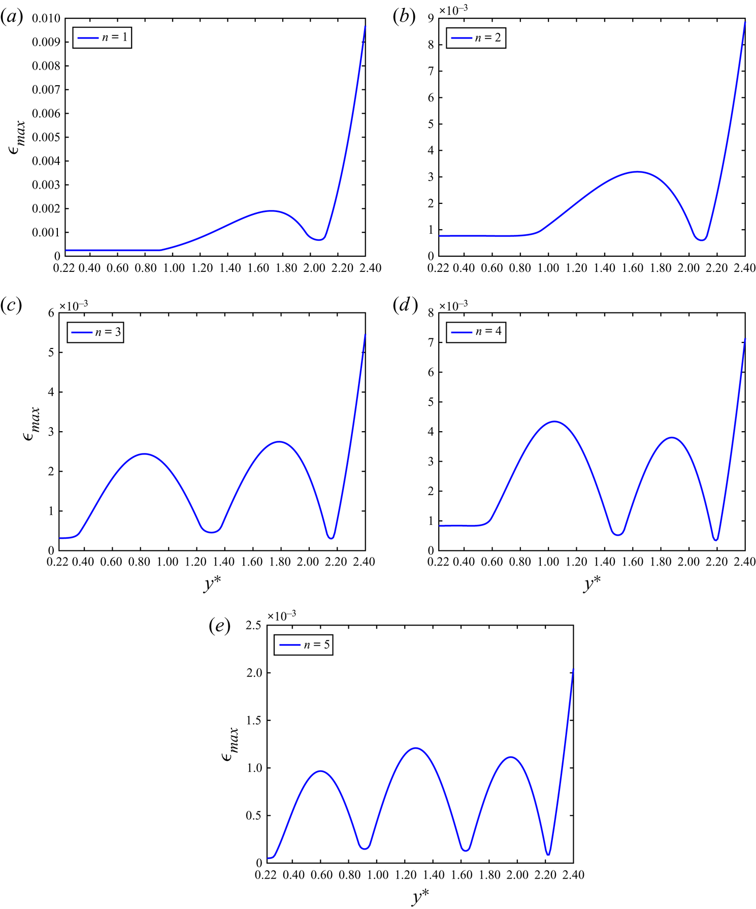
 $\epsilon _{max}(y)$ is shown for the first five hydroelastic waves where
 $k^*=0.5$,
 $a^*=0.22$ and
 $h^*=0.01$. It is seen that the distributions
 $\epsilon _{max}(y)$ peak at the walls,
 $y^*=2.4$, for
 $n=1,2,3,4,5$. The strains near the free edge of the ice sheet are small, compare with figure 17. For the conditions of the hydroelastic waves in this figure, cracks are expected along the walls if the strain is greater than the so-called yield strain
 $\epsilon _Y$. The yield strain for ice is estimated as
 $8\times 10^{-5}$ (Brocklehurst, Korobkin & Parau Reference Brocklehurst, Korobkin and Parau2011). Figure 19(a) shows that the strains in the ice plate caused by the lowest hydroelastic wave are below the yield strain for ice if the magnitude of this wave is smaller than
 $8\,\mathrm {mm}$. These cracks along the walls may break the connection between the ice sheet and the walls without breaking the ice sheet into pieces.
Distributions of the strains  $\epsilon _{max}(y)$ across the channel,
 $a^*=0.22$,
 $h^*=0.01$ in the hydroelastic waves with
 $k^*=0.5$.

7. Conclusions
The effect of a lead of open water on the hydroelastic waves propagating in an ice channel was studied within the linear theory of hydroelasticity. The normal mode method and the eigenfunction expansion method were used to determine the dispersion relations and the profiles of these waves for elastic ice and rigid ice models, respectively. Only waves symmetric with respect to the centreplane of the channel were considered. It was shown that the presence of a lead significantly changes the waves propagating along the ice channel. In a channel completely covered with an ice plate, short waves propagate through the ice with water in the channel being less involved in the motion. These waves are elastic waves. Very long waves in an ice channel depend on the presence of ice only in a closed proximity of the walls of the channel, where the ice plate is clamped to the walls. However, the dispersion relations are affected by the ice cover even for very long waves, if the ice thickness is moderate. Hydroelastic waves are in between very long waves, which are gravity dominated, and short waves, which are dominated by the ice elasticity. The interplay between gravity and elastic effects makes these waves particular with the most prominent feature being the existence of a single so-called critical speed for each mode of the waves in the ice channel.
The presence of a lead in the ice channel changes the short waves. They are gravity waves now. They are confined to the part of the channel under the lead with ice deflections being negligible. Moreover, the flow between the region under the ice and the region under the lead becomes negligible for higher modes of the waves. The lead also modifies the hydroelastic waves, which are long enough for both gravity and elastic effects being equally important. The most important modification is related to the critical speeds of these waves. Each wave mode starting from the lowest one can have zero, one, two or even more critical speeds depending on the relative width of the lead. At some particular conditions two critical speeds may merge providing a point on the dispersion curve, where both the first and second derivatives of the phase speed with respect to the wavenumber are zero. At that point, the phase speed is equal to the group speed and the second derivative of the wave frequency as a function of the wavenumber is zero. Waves propagating at a critical speeds cannot be linear. They are described by the nonlinear Schrodinger equation for small amplitudes and can be computed for moderate wave amplitudes. The second derivative of the wave frequency,  $\frac {1}{2}(\omega _n^*(k^*))''$, appears as the coefficient of the dispersion term in the nonlinear Schrodinger equation. If two critical speeds merge, this coefficient becomes zero, which would require revision of the weakly nonlinear hydroelastic waves in such special conditions. In our analysis, we did not find conditions where three or more critical speeds merge; however, potentially this is possible making the theory of weakly nonlinear hydroelastic waves even more challenging.
The present study can be easily extended to cases involving free or simply supported edges at the lateral ends of the channel, through modifying the boundary conditions at  $\tilde {y}=0$ in (A2) to free or simply supported boundary conditions, and solving the corresponding eigenfunctions
 $\widetilde {\psi _n}(\tilde {y})$. The present study is also planned to be extended further including asymmetric waves for different positions of a lead in the ice channel, and to be applied to the problem of a load moving along an ice channel either in the lead or on the ice cover near the lead. Motions of loads at critical speeds and generated stresses in the ice cover will receive special attention. We are unaware of results for the conditions, where two or more critical speeds merge. It would be challenging to describe the ice response to a load moving at such a special speed.
Acknowledgements
This research was started when the first author was visiting the School of Mathematics, University of East Anglia as an academic visitor in the period from December 2019 to May 2020. The authors are thankful to Prof. E.I. Parau for fruitful discussions of nonlinear hydroelastic waves and to anonymous referees for their valuable suggestions on the interpretation of the obtained results and their presentations.
Funding
This work is supported by National Key R&D Program of China (No. 2017YFE0111400) and by National Natural Science Foundation of China (Nos. 51979051, 51979056 and 51639004).
Declaration of interests
The authors report no conflict of interest.
Appendix A. Elastic modes  $\psi _n(y)$

Here we take the second equation of (3.2) as an example to illustrate how to solve the eigenvalue problem in dimensionless variables. It is convenient to write the second equation of (3.2) in dimensionless variables,  $\tilde {y}=(y-L)/\ell$,
 $\tilde {\psi }_n(\tilde {y})=\sqrt {\ell }\psi _n(\tilde {y} \ell +L)$, denoted by tilde. Here
 $\ell =L-a$ is the width of each ice plate. The dimensionless problem reads as
 \begin{gather} \left(\dfrac{\mathrm{d}^2}{\mathrm{d}\tilde{y}^2}-\tilde{k}^2\right)^2\tilde{\psi}_n =\tilde{\lambda}_n^{4}\tilde{\psi}_n \quad ({-}1<\tilde{y}<0), \end{gather}
 \begin{gather}\tilde{\psi}_n(0)=\tilde{\psi}_n'(0)=0, \quad \tilde{\psi}_n''({-}1)=\nu \tilde{k}^2 \psi_n({-}1), \quad \tilde{\psi}_n'''({-}1)=(2-\nu) \tilde{k}^2 \tilde{\psi}_n'({-}1), \end{gather}
where  $\tilde {k}=k\ell$ and
 $\tilde {\lambda }_n=\lambda _n \ell$. For
 $\tilde {k}=0$, this problem provides the shape functions of eigen vibrations of a cantilever beam, which is clamped at
 $\tilde {y}=0$ and free-free at
 $\tilde {y}=-1$; see Timoshenko & Young (Reference Timoshenko and Young1955). The non-zero solutions of the problem (A1), (A2) for
 $\tilde {k}=0$ exist for
 $\lambda _n$, which satisfy the equation
 $\cos {\tilde {\lambda }_n}\cdot \cosh {\tilde {\lambda }}_n=-1$.
For  $\tilde {k}>0$, the non-zero solutions of (A1), (A2) are given by (Eastham (Reference Eastham1970))
 \begin{equation} \tilde{\psi}_n(\tilde{y})= A_n \left[ \dfrac{\sin q\tilde{y}}{q} -\dfrac{\sinh p\tilde{y}}{p} +Q(\tilde{\lambda}_n) \cos q\tilde{y} - Q(\tilde{\lambda}_n) \cosh p\tilde{y} \right], \end{equation}
where  $p=\sqrt {\tilde {\lambda }_n^2+\tilde {k}^2}$,
 $q=\sqrt {\tilde {\lambda }_n^2-\tilde {k}^2}$,
 \begin{equation} Q(\tilde{\lambda}_n)=\dfrac{[\tilde{\lambda}_n^2+ (1-\nu)\tilde{k}^2] \dfrac{ \sinh p}{p} + [\tilde{\lambda}_n^2- (1-\nu)\tilde{k}^2] \dfrac{ \sin q}{q}}{[\tilde{\lambda}_n^2+(1-\nu)\tilde{k}^2] \cosh p+ [\tilde{\lambda}_n^2- (1-\nu)\tilde{k}^2] \cos q}, \end{equation}
and the coefficients  $A_n$ are determined by the second equation of (3.3a,b),
 \begin{align} \dfrac{1}{A_n^2} &={-} 2Q \left[ \dfrac{\sin^2 q}{2q^2}+ \dfrac{\sinh^2 p}{2p^2}- \dfrac{\sinh p \sin q}{pq} \right] \nonumber\\ &\quad +Q^2 \left[ 1+\dfrac{\sin q \cos q}{2q}+ \dfrac{\sinh p \cosh p}{2p}- 2\dfrac{q \cosh p \sin q+ p\sinh p \cos q}{p^2+q^2} \right] \nonumber\\ &\quad + \left[ \dfrac{p^2-q^2}{2p^2 q^2}+ \dfrac{\sinh p \cosh p}{2p^3}- \dfrac{\sin q \cos q}{2q^3}- 2\dfrac{p\cosh p \sin q- q\sinh p \cos q}{pq(p^2+q^2)} \right]. \end{align}
These non-zero solutions exist for  $\tilde {\lambda }_n$ which are real and positive roots of the equation
 \begin{equation} \dfrac{\tilde{\lambda}_n^4-(1-\nu)^2\tilde{k}^4}{\tilde{\lambda}_n^4+(1-\nu)^2\tilde{k}^4} + \cosh p \cos q = \left[\tilde{k}^2- \dfrac{2\tilde{\lambda}_n^4(1-\nu)\tilde{k}^2}{\tilde{\lambda}_n^4+(1-\nu)^2\tilde{k}^4} \right] \dfrac{\sinh p}{p} \dfrac{\sin q}{q}. \end{equation}
Equations (A3)–(A6) are written for  $\tilde {\lambda }_n>\tilde {k}$. For
 $\tilde {\lambda }_n=\tilde {k}$, one needs to change
 $\cos {(\sqrt {\tilde {\lambda }_n^2-\tilde {k}^2})}$ and
 $\sin {(\sqrt {\tilde {\lambda }_n^2-\tilde {k}^2})}/{(\sqrt {\tilde {\lambda }_n^2-\tilde {k}^2})}$ to
 $1$. For
 $\tilde {\lambda }_n<\tilde {k}$, one needs to change
 $\cos {(\sqrt {\tilde {\lambda }_n^2-\tilde {k}^2})}$ to
 $\cosh {(\sqrt {\tilde {k}^2-\tilde {\lambda }_n^2})}$ and
 $\sin {(\sqrt {\tilde {\lambda }_n^2-\tilde {k}^2})}/(\sqrt {\tilde {\lambda }_n^2-\tilde {k}^2})$ to
 $\sinh {(\sqrt {\tilde {k}^2-\tilde {\lambda }_n^2})}/ (\sqrt {\tilde {k}^2-\tilde {\lambda }_n^2})$. The roots of (A6),
 $\tilde {\lambda }_n(\tilde {k})$,
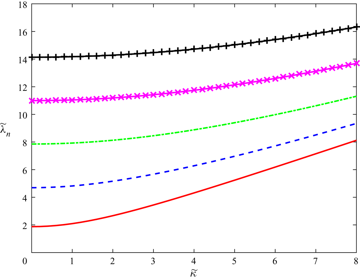
 $n=1,2,3,4,5$, are shown in figure 20 as functions of the dimensionless wavenumber
 $\tilde {k}$ for
 $\nu =0.3$. Note that
 $\tilde {\lambda }_{n+1}(\tilde {k})>\tilde {\lambda }_n(\tilde {k})$ for
 $\tilde {k} \geq 0$ and
 $n\geq 1$. In particular,
 $\tilde {\lambda }_1(\tilde {k})=\tilde {k} \approx 23.413$ for
 $\nu =0.3$.
The dimensionless spectral parameters  $\tilde {\lambda }_n$ as functions of the dimensionless wavenumber
 $\tilde {k}$ for
 $\nu =0.3$ and
 $n=1,2,3,4,5$.

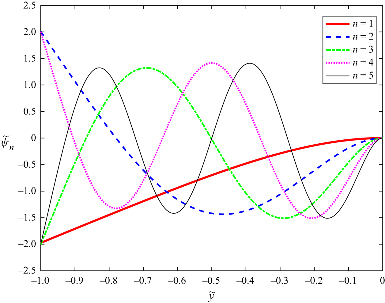
The shape functions  $\tilde {\psi }_n(\tilde {y})$ defined by (A3)–(A6) are shown in figure 21 for
 $\tilde {k}=1$,
 $\nu =0.3$ and
 $n=1,2,3,4,5$. These shape functions,
 $\tilde {\psi }_n(\tilde {y})$, have
 $n-1$ zeros inside the interval
 $(-1,0)$, where
 $\tilde {y}=0$ corresponds to the clamped edge of the ice plate.
The dimensionless normalised shape functions  $\tilde {\psi }_n(\tilde {y})$ for
 $\tilde {k}=1$,
 $\nu =0.3$ and
 $n=1,2,3,4,5$.

Appendix B. The integrals $\tilde {A}_{nr}$ from § 3

The method of separating variables applied to the boundary problem (3.7) and (3.8a,b) provides
 \begin{equation} \varPhi_n(y,z)=\sum_{m=1}^{\infty} D_{nm} \dfrac{\cosh[\sqrt{k^2+\mu_m^2}(z+H)]}{\cosh[\sqrt{k^2+\mu_m^2}H]}\cos(\mu_m y), \end{equation}
where  $\mu _m={\rm \pi} (m-1)/L$, the coefficients
 $D_{nm}$ are determined using the boundary condition (3.13),
 \begin{equation} \sum_{m=1}^{\infty} D_{nm} \left(\sqrt{k^2+\mu_m^2}\tanh[\sqrt{k^2+\mu_m^2}H]-\dfrac{\omega^2}{g}\right)\cos(\mu_m y)=\psi_n(|y|){\mathcal{H}}(y^2-a^2). \end{equation}
Here  ${\mathcal {H}}(x)$ is the Heaviside function, which is equal to zero for negative
 $x$ and one for positive
 $x$. The functions
 $\cos (\mu _m y)$,
 $m\geq 1$, are orthogonal in the interval
 $-L\lt y\lt L$,
 \begin{equation} \int_{{-}L}^L \cos(\mu_m y)\cos(\mu_r y) \,\mathrm{d} y= \left\{\begin{array}{@{}ll} 0, & r\neq m, \\ L, & r=m\neq 1, \\ 2L, & r=m=1. \end{array} \right. \end{equation}
Multiplying both sides of (B2) by  $\cos (\mu _r y)$ and integrating the result in
 $y$ from
 $-L$ to
 $L$ using the relations (B3), we find that
 \begin{equation} D_{nm}=\dfrac{\epsilon_m}{L\left[\sqrt{k^2+\mu_m^2}\tanh[\sqrt{k^2+\mu_m^2}H]-\omega^2/g\right]}\int_a^L \psi_n(y)\cos(\mu_m y) \,\mathrm{d} y, \end{equation}
where  $\epsilon _1=1$ and
 $\epsilon _m=2$ for
 $m\geq 2$. The denominators in (B4) are not equal to zero in our computations for a channel with ice cover and a lead because we do not consider the frequencies
 $\omega =\omega ^{(f)}_m(k)=\sqrt {g\sqrt {k^2+\mu _m^2}\tanh [\sqrt {k^2+\mu _m^2}H]}$, which correspond to the frequencies of water waves in the channel without ice.
Denote the integrals in (B4) by  $S_{nm}$. Then (B1) and (B4) give the integrals from § 3,
 \begin{equation} \tilde{A}_{nr}=\int_a^L \varPhi_n(y,0)\psi_r(y) \,\mathrm{d} y= \sum_{m=1}^{\infty} \dfrac{\epsilon_m S_{nm}S_{rm}}{L\left[\sqrt{k^2+\mu_m^2}\tanh[\sqrt{k^2+\mu_m^2}H]-\omega^2/g\right]}. \end{equation}
With the help of integration by parts one can show that  $S_{nm}\sim -\psi _n(a)\sin (\mu _m a)/\mu _m$ as
 $m\to \infty$. Therefore, the terms in the series (B5) decay as
 $m^{-3}$ for
 $m\to \infty$. The integrals
 $S_{nm}$ are evaluated by multiplying both sides of the second equation of (3.2) by
 $\cos (\mu _m y)$ and integrating the result in
 $y$ from
 $a$ to
 $L$ by parts using the edge conditions from the second equation of (3.2), which gives
 \begin{equation} \int_a^L \left(\dfrac{\mathrm{d}^2}{\mathrm{d} y^2}-k^2\right)^2\psi_n \cos(\mu_m y)\,\mathrm{d} y=\int_a^L \lambda_n^4\psi_n \cos(\mu_m y)\,\mathrm{d} y, \end{equation}
and
 \begin{equation} S_{nm}=\dfrac{({-}1)^m\psi_n'''(L)\!+\!(\mu_m^2+\nu k^2)\cos(\mu_m a)\psi_n'(a)\!+\! \mu_m[(2-\nu)k^2\!+\!\mu_m^2]\sin(\mu_m a)\psi_n(a)}{\lambda_n^4-(k^2\!+\!\mu_m^2)^2}. \end{equation}
Using the dimensionless variable from Appendix A,  $y=\tilde {y} \ell +L$, where
 $\ell =L-a$, multiplying (B7) by
 $\ell ^4$ in the numerator and denominator, and denoting
 $\mu _m \ell ={\rm \pi} (m-1)(1-a/L)$ by
 $\tilde {\mu }_m$, we find that
 \begin{align} S_{nm}&= \dfrac{\sqrt{\ell}}{\tilde{\lambda}_n^4-(\tilde{k}^2+\tilde{\mu}_m^2)^2} [({-}1)^m \tilde{\psi}_n'''(0) &+& \tilde{\mu}_m[(2-\nu)\tilde{k}^2 +\tilde{\mu}_m^2]\sin(\mu_m a)\tilde{\psi}_n({-}1) \nonumber\\ &\quad +(\tilde{\mu}_m^2+\nu \tilde{k}^2)\cos(\mu_m a)\tilde{\psi}_n'({-}1)], \end{align}
where the modes  $\tilde {\psi }_n(y)$ and the eigenvalues
 $\tilde {\lambda }_n$ are defined in Appendix A.