1 Introduction
Wind energy has emerged as one of the fastest-growing renewable energy resources in recent decades (Leung & Yang Reference Leung and Yang2012; Zheng et al.
Reference Zheng, Li, Pan, Liu and Xia2016). With the exponential increase in size, the modern wind turbines rise above 100 m, occupying a substantial portion of the atmospheric boundary layer (ABL). The turbulent flows around these gigantic structures impose unprecedented challenges for the research community to implement the knowledge from laboratory research in industrial applications. Despite past research efforts, as reviewed by a number of publications (Leishman Reference Leishman2002; Snel Reference Snel2003; Vermeer, Sorensen & Crespo Reference Vermeer, Sorensen and Crespo2003; Sanderse, van der Pijl & Koren Reference Sanderse, van der Pijl and Koren2011; Sørensen Reference Sørensen2011a
,Reference Sørensen
b
), the complex flows around utility-scale turbines and multi-turbine arrays remain poorly understood, which contributes to sub-optimal performance at the plant scale and an average power loss of 10 %–20 % (Barthelmie et al.
Reference Barthelmie, Frandsen, Nielsen, Pryor, Rethore and Jørgensen2007, Reference Barthelmie, Hansen, Frandsen, Rathmann, Schepers, Schlez, Phillips, Rados, Zervos, Politis and Chaviaropoulos2009). Such loss, referred to as wake loss, is caused by wind turbines in wind farm interacting with the turbulent wake flows from upstream turbines which carry less kinetic energy and intensified turbulence. In addition, the wake-generated turbulence is a major source of fatigue loading, which drives premature component failure, results in expensive over-design criteria and limits the turbine and wind farm innovation potential (Frandsen et al.
Reference Frandsen, Barthelmie, Pryor, Rathmann, Larsen and Højstrup2006; Musial, Butterfield & McNiff Reference Musial, Butterfield and McNiff2007; Sheng & Veers Reference Sheng and Veers2011). According to the literature (Vermeer et al.
Reference Vermeer, Sorensen and Crespo2003; Göçmen et al.
Reference Göçmen, Van Der Laan, Réthoré, Diaz, Larsen and Ott2016), a wind turbine wake is generally divided into the near wake, within 1–4
 $D$
(
 $D$
– rotor diameter) behind the turbine, and the far wake, the region beyond the near wake, where the influence of rotor properties is less important. In particular, in the near wake, the flow field is strongly dependent on rotor properties and turbine operations and is dominated by turbine-generated coherent structures such as blade tip and root vortices, trailing vortex sheets, hub vortices and tower vortices, etc. As pointed out in Sørensen (Reference Sørensen2011b
), the interaction of these structures in the near wake affects the evolution and turbulent flow characteristics of the far wake. Therefore, a better understanding of the dependence of near-wake flow characteristics on turbine operation and incoming flow can yield a more accurate prediction of wake growth and provide guidance for developing ‘smart’ control to reduce wake loss and structural impact for future wind farms. Investigation of the near wake of utility-scale wind turbines has been conducted using analytical modelling, laboratory and field experiments as well as numerical simulations. So far, the analytical studies of the near wake are focused on examining the stability of coherent structures (Widnall Reference Widnall1972; Gupta & Loewy Reference Gupta and Loewy1974; Okulov Reference Okulov2004; Okulov & Sørensen Reference Okulov and Sørensen2007), and the current analytical/empirical models of the wake growth generally ignore the intricate details of the near wake (e.g. Jensen Reference Jensen1983, Ainslie Reference Ainslie1988). For example, Widnall (Reference Widnall1972) studied a helical vortex filament and its stability under small disturbances analytically, capturing three modes of instability on a disturbed helical vortex filament. To analyse the stability of the wake behind a multi-bladed rotor wind turbine, Okulov & Sørensen (Reference Okulov and Sørensen2007) implemented linear stability analysis on a vortex system which includes helical tip, root and hub vortices, showing that the stability of tip vortices strongly depends on the radial extent of hub vorticity as well as on the type of vorticity distribution. This work highlighted the necessity to consider all vortex structures within the near wake for a realistic analysis of the stability of the wake. Regarding the wake modelling, the wake velocity profiles predicted by the popular wake models (Jensen Reference Jensen1983; Katic, Højstrup & Jensen Reference Katic, Højstrup and Jensen1986; Ainslie Reference Ainslie1988; Frandsen et al.
Reference Frandsen, Barthelmie, Pryor, Rathmann, Larsen and Højstrup2006) are based on simplified mass and momentum conservation with an unrealistic top-hat shape for the velocity deficit (Bastankhah & Porté-Agel Reference Bastankhah and Porté-Agel2014). Accordingly, as pointed out in a recent review paper on wake models (Göçmen et al.
Reference Göçmen, Van Der Laan, Réthoré, Diaz, Larsen and Ott2016), such simplification of the near-wake profiles could result in substantial uncertainty in the prediction of wake behaviours. Overall, these analytical studies generally involve substantial simplifications on flow characteristics, rotor properties and turbine operation, and do not take into account the complexity of the atmospheric environment. Although they can provide some fundamental guidance, their implementation to utility-scale turbines is either significantly limited or requires considerable empirical correction.
The laboratory studies of the near wake are generally based on experiments with small-scale turbine models in wind and water tunnels. With particle image velocimetry (PIV), a number of studies provided detailed quantification of the near-wake velocity field and turbulent statistics as well as coherent structure behaviours (Hu, Yang & Sarkar Reference Hu, Yang and Sarkar2012; Sherry et al.
Reference Sherry, Nemes, Lo Jacono, Blackburn and Sheridan2013a
; Sherry, Sheridan & Lo Jacono Reference Sherry, Sheridan and Lo Jacono2013b
; Nemes et al.
Reference Nemes, Lo Jacono, Blackburn and Sheridan2015). For example, Hu et al. (Reference Hu, Yang and Sarkar2012) used PIV with a phase-lock technique to investigate the velocity field downstream of a model turbine in a wind tunnel. Their study provided a quantification of the velocity profile and turbulent statistics in the near wake and indicated a strong correlation between the peak of turbulent kinetic energy (TKE) and the region influenced by coherent structures like blade tip and root vortices. In a water channel, to investigate the generation and evolution of the helical structure of the wind turbine, Sherry et al. (Reference Sherry, Nemes, Lo Jacono, Blackburn and Sheridan2013a
) studied the behaviours of the tip and root vortices of a wind turbine model utilizing phase-locked two-dimensional PIV. The relationship between the helical vortex system and the governing parameters of the system was explored. With the same experimental set-up, Sherry et al. (Reference Sherry, Sheridan and Lo Jacono2013b
) further investigated the wake of the wind turbine model for both the upwind and downwind configurations by examining the helicoidal pitch and vortex circulation under different tip speed ratios with special attention to the development of root vortices. The root vortex signatures were found to persist only in the extreme near-wake regions (less than 0.25
 $D$
) indicating strong diffusion characteristics. Nevertheless, the scaling of the findings from these laboratory-scale studies to utility-scale turbines is strongly limited by the significant difference in Reynolds number, atmospheric conditions (e.g. turbulence, shear and stratification) as well as the properties of turbine models (i.e. geometry, mechanical response and turbine operation) between laboratory and field applications.
Compared to laboratory studies, the field measurements can provide direct quantification of wind turbine wake flows at utility scale, but have usually very limited spatial and/or temporal resolution. The conventional field measurement techniques for atmospheric flows include meteorological towers instrumented with single-point wind velocity sensors (e.g. sonic, cup-and-vane), and various wind profiling instruments such as lidar, sodar and radar, etc. With the integration of multiple profiling instruments and innovative scanning schemes, a number of recent field studies have provided an unprecedented characterization of utility-scale turbine wakes (Iungo, Wu & Porté-Agel Reference Iungo, Wu and Porté-Agel2012; Hirth et al. Reference Hirth, Schroeder, Gunter and Guynes2015; Kumer et al. Reference Kumer, Reuder, Dorninger, Zauner and Grubisic2016). For example, Iungo et al. (Reference Iungo, Wu and Porté-Agel2012) conducted scanning Doppler lidar measurements with 18 m spatial resolution in the wake of a 2-MW turbine and showed high turbulence characteristics within the near wake. Turbulence intensity as high as 30 % was observed at the turbine top tip level up to three rotor diameters downstream. Nevertheless, the implementation of these techniques in the near wake is significantly limited by their spatio-temporal resolution, which is insufficient to resolve the rich coherent structures generated by the turbine and their interactions. Such information is important for elucidating the physical mechanisms governing wake growth and other behaviours of the wake (e.g. wake meandering) for utility-scale turbines.
Taking advantage of natural snowfalls, Hong et al. (Reference Hong, Toloui, Chamorro, Guala, Howard, Riley, Tucker and Sotiropoulos2014) implemented super-large-scale PIV (SLPIV) and flow visualization with natural snowflakes to study, for the first time, the complex flow field and coherent structures in the near wake of a 2.5 MW wind turbine. This study revealed the rich interaction of tip vortices and quantified a flow field of approximately
 $36\times 36~\text{m}^{2}$
at
 ${\sim}0.3D$
from the rotor. In addition, this study also demonstrated the strong correlation between the high-resolution instantaneous flow field and turbine operation parameters. However, due to the constraints of measurement capacity, the near-wake flow fields obtained in the seminal study were limited to the elevation span of the lower-blade tip, far from an adequate characterization of the entire near wake. Moreover, the experiment only had a sample duration of the flow field and the tip vortex visualization for a few minutes, limiting statistical investigation over a wide range of turbine operational and flow conditions.
With the advancement of computational power, high-fidelity numerical simulations have been used extensively to investigate the fundamental physical processes in turbine wake flows. In particular, a number of large eddy simulation (LES) studies were conducted recently to provide physical insights into the near wake. For example, Kang, Yang & Sotiropoulos (Reference Kang, Yang and Sotiropoulos2014) conducted a systematic investigation on the wake meandering of a hydrokinetic turbine using actuator disk, line and turbine resolving LES techniques, and pointed out that turbine hub and tip vortex interaction in the near-wake region (less than 3
 $D$
) triggered wake meandering on a hydrokinetic turbine. Ivanell et al. (Reference Ivanell, Leweke, Sarmast, Quaranta, Mikkelsen and Sørensen2015) studied the flow in the near-wake region on a turbine model by comparing the LES simulation and experimental results, showing a good agreement between the results from the two approaches. Inspired by the measurement data from Hong et al. (Reference Hong, Toloui, Chamorro, Guala, Howard, Riley, Tucker and Sotiropoulos2014), Yang et al. (Reference Yang, Hong, Barone and Sotiropoulos2016) investigated in detail the peculiar elongated tip vortex patterns in the near wake using LES, and revealed the formation of secondary counter-rotating spiral vortices which arise out of centrifugal instability mechanisms within the tip vortex shear layers. However, this study did not examine the connection between tip vortex behaviour and turbine operational parameters. It is noteworthy that the current numerical simulations of utility-scale turbines are solver dependent and cannot incorporate complete turbine geometrical characteristics due to computational constraints. In addition, the effects of the real atmospheric environment and highly dynamic response (e.g. aeroelasticity) of the utility-scale turbines are very difficult to capture in the current simulations.
The current paper presents the continuation of our field measurements from Hong et al. (Reference Hong, Toloui, Chamorro, Guala, Howard, Riley, Tucker and Sotiropoulos2014) using SLPIV and flow visualization with natural snowflakes. In particular, by combining the data from multiple field campaigns from 2014 to 2016, we overcome the limitation of Hong et al. (Reference Hong, Toloui, Chamorro, Guala, Howard, Riley, Tucker and Sotiropoulos2014) in the study of the near-wake behaviours of a utility-scale turbine. The paper is structured as follows: § 2 provides a brief description of the experimental methods, field campaigns and data process procedures. Section 3.1 reports the results of the near-wake velocity field spanning from the blade-bottom tip to the top tip with unprecedented spatio-temporal resolution using the data from the field campaign in February 2016. Section 3.2 reports a statistical analysis of the connection of tip vortex behaviours with turbine operational and flow conditions in the near wake combining the data from all the field campaigns from 2014–2016. Section 4 provides a summary and discussion of the results.
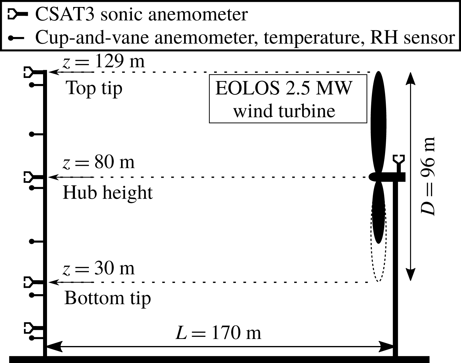
Schematic of the 2.5 MW turbine and the met tower at EOLOS station.
2 Experimental method
The field experiments are conducted at EOLOS Wind Energy Research Field Station (referred to as the EOLOS station hereafter) in Rosemount, MN. As shown in figure 1, the EOLOS station consists of a 2.5 MW Clipper Liberty C96 wind turbine (referred to as the EOLOS turbine hereafter) and a 130 m meteorological tower (referred to as the met tower hereafter). The EOLOS turbine is a 3-bladed, horizontal-axis, a pitch-regulated machine with a rotor diameter (
 $D$
) of 96 m and a supporting tower 80 m in height, capable of operating at variable wind speed. The EOLOS turbine has the standard instrumentation to record turbine operational conditions and rotor instrumentation including accelerometers and strain gauges installed on each blade for characterizing blade deformations as well as tower instrumentation comprised of strain gauges mounted at the tower base for quantifying structural response. The met tower, located 170 m (corresponding to
 ${\sim}1.77D$
) south of the turbine (as the south is the predominant wind direction), is designed to characterize the atmospheric conditions during the operation of the EOLOS turbine. Note that this distance is slightly different from the value (i.e. ‘160 m’) presented in previous publications using the EOLOS facility. This adjustment is made according to a recent field survey that precisely calibrated the location of the EOLOS turbine and the met tower. The met tower instrumentation includes a number of wind velocity (sonic, cup-and-vane anemometers), temperature and humidity sensors installed at elevations ranging from 7 m to the highest point of the rotor, 129 m. Four of these elevations (129, 80, 30 and 10 m) are instrumented with high resolution, Campbell Scientific CSAT3 3D sonic anemometers with a sampling rate of 20 Hz. These four heights were selected to match the rotor top, rotor hub, rotor bottom and standard 10 m height. Three metres below each of the CSAT3’s (elevations of 126, 77, 27 and 7 m) and at points representing elevations at the midpoint between the edge of the rotor and hub height (105 and 55 m) are standard cup-and-vane anemometers. Overall, the data from the instrumentation on the EOLOS turbine and the met tower, including turbine operational conditions (e.g. power, blade pitch and tip-speed-ratio, etc.) and turbine structural response (e.g. blade and tower base strain, etc.) and atmospheric conditions are sampled continuously 24 h a day and stored on backed up servers. The detailed information of the facility and the instrumentation at the EOLOS station is provided in the supplemental document of Hong et al. (Reference Hong, Toloui, Chamorro, Guala, Howard, Riley, Tucker and Sotiropoulos2014).
The experiments employ the SLPIV and flow visualization approach from Hong et al. (Reference Hong, Toloui, Chamorro, Guala, Howard, Riley, Tucker and Sotiropoulos2014) to investigate the flow field and the coherent structures in the near wake. Briefly, the experimental set-up is composed of an optical assembly for illumination, a camera and the corresponding data acquisition system. The optical assembly includes a 5 kW highly collimated search light (a divergence
 ${<}0.3^{\circ }$
and initial beam size of 300 mm in diameter) and a curved reflecting mirror for projecting a horizontal cylindrical beam into a vertical light sheet. The sheet expansion angle is controlled by adjusting the mirror curvature. The illumination system is affixed to a trailer, providing good mobility for aligning the light sheet with the predominant flow direction, as required for planar PIV measurements. To yield better light sensitivity for recording the flow field over a larger sampling area, we replaced the camera system used in Hong et al. (Reference Hong, Toloui, Chamorro, Guala, Howard, Riley, Tucker and Sotiropoulos2014) with the Sony-A7RII camera. The camera, mounted with a 50 mm
 $f/1.2$
lens, can provide 4K-resolution 30 Hz videos with continuous data recording for approximately 30 min, sufficient for recording large-scale turbulent flows in the atmospheric boundary layer (ABL). The original SLPIV technique using natural snowflakes was validated through a comparison with the sonic measurements at different elevations of the met tower at the EOLOS station in Toloui et al. (Reference Toloui, Riley, Hong, Howard, Chamorro, Guala and Tucker2014). Recently, the updated experimental set-up has been employed to study the settling behaviour of snowflakes within a field of view (FOV) of 7 m
 $\times$
4 m in the ABL at the EOLOS station (Nemes et al.
Reference Nemes, Dasari, Hong, Guala and Coletti2017). The snowflake trajectories were successfully analysed using two-dimensional particle tracking velocimetry (PTV), which revealed an enhanced the settling behaviour of the snowflakes due to atmospheric turbulence. These studies substantiate the efficacy and robustness of our techniques for full-scale turbulent flow studies in the atmospheric environment.
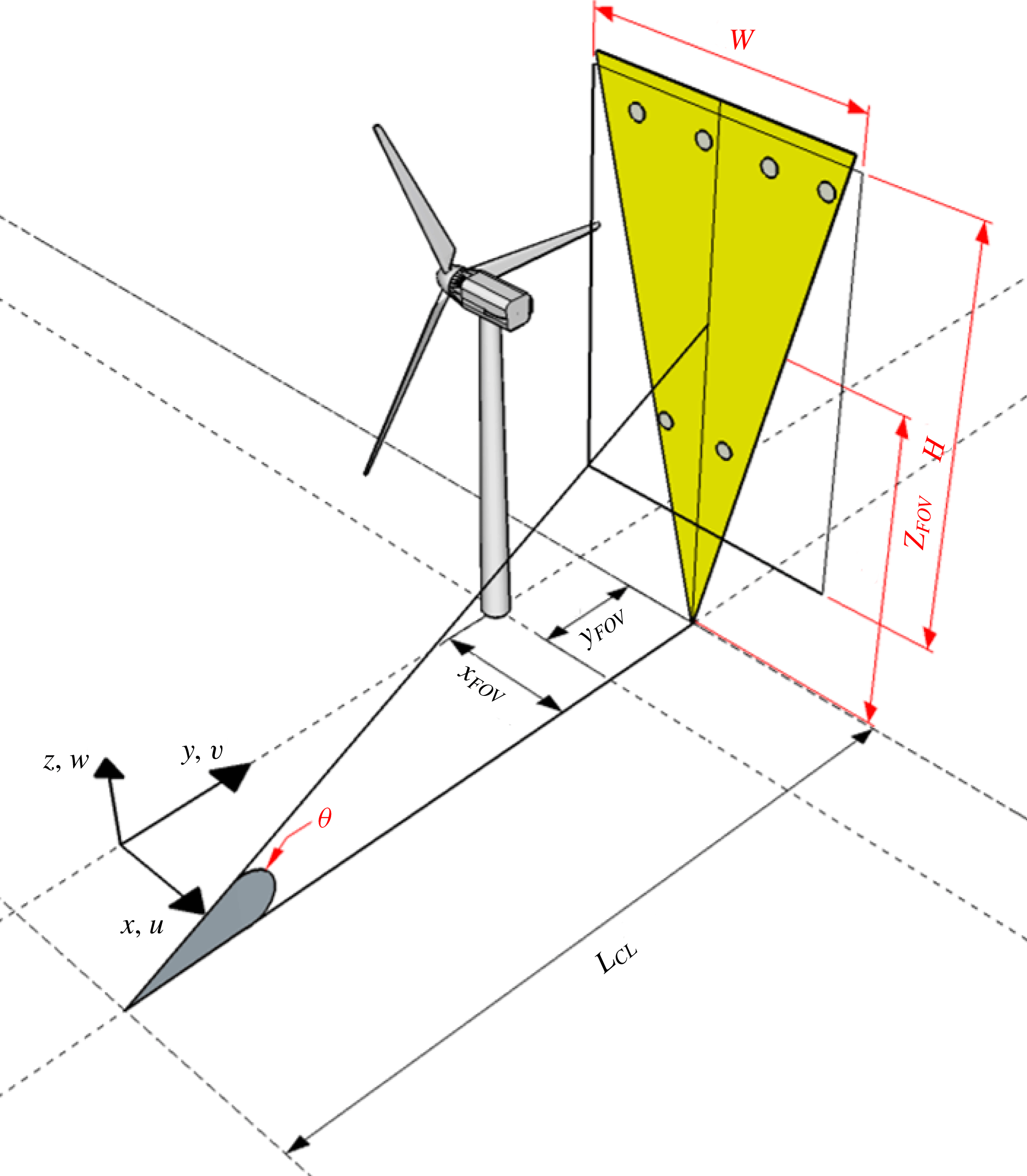
The present paper uses five datasets obtained from four deployments in the past three years. The information for each dataset is summarized in tables 1 and 2 with a schematic presented in figure 2 illustrating the key parameters for the measurement set-up. Specifically, as shown in table 1 and figure 2, the location of the FOV for each dataset is characterized by its downstream distance from the tower (
 $x_{FOV}$
), its offset from the central tower plane (
 $y_{FOV}$
) and the elevation of the FOV centre above the ground level (
 $z_{FOV}$
). The dimensions of the FOV are characterized by its height (
 $H$
) and width (
 $W$
). The distance between the camera and the light sheet is represented by
 $L_{CL}$
with
 $\unicode[STIX]{x1D6E9}$
indicating the tilt angle of the camera. Among all the five datasets, the Feb 2016b dataset has the largest FOV which covers the entire wake flow field on the streamwise-vertical (xz) plane located at 0.19
 $D$
offset from the central tower plane. This dataset is exclusively used for quantitative examination of the near-wake turbulent flow field. The rest of the datasets, with a smaller FOV covering the region where the turbine blade intersects with the light sheet plane near the bottom of its revolution (referred to as the bottom tip elevation), are used to investigate the tip vortex behaviours and their correlations with the turbine operation/response. Table 2 summarizes the detailed meteorological information as well as the turbine operational conditions for all the datasets. The wind speed and direction are measured by the sonic anemometer at the nacelle of the EOLOS turbine. Temperature and humidity are measured at the met tower. The turbulence intensity and Obukhov length are calculated from the acquired data accordingly. Note that the turbulence intensity and the Obukhov length are not available for the Apr 2014 dataset due to the failure of the acquisition system for the measurements from the nacelle and the met tower during the deployment.
A summary of the key parameters of the measurement set-up for each deployment dataset used in the present paper. Each dataset is referred to by the month and the year when the dataset was obtained, i.e. ‘Apr 2014’ – the dataset obtained on 3 April, 2014, ‘Nov 2015’ – the dataset obtained on 30 November, 2015, ‘Dec 2015’ – the dataset obtained on 28 December, 2015, ‘Feb 2016a’ – one small FOV dataset obtained on 2 February, 2016, ‘Feb 2016b’ – one large FOV dataset obtained on February 2nd, 2016.

A summary of the key parameters of the atmospheric and turbine operational conditions. RH – relative humidity,
 $L$
– Obukhov length, TSR – ratio of the tangential speed of the blade tip to the incoming wind speed. Note that the turbine operational region is a state of turbine operation based on the rotor speed and power constraints on the turbine and is determined by the incoming wind speed and the control strategy.

Schematic of the measurement set-up used in the deployments.
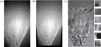
A sample of (a) raw image, (b) de-warped image and (c) enhanced image after background subtraction showing the steps of image processing before the velocity vector calculation. Insets in (c) demonstrate the various snow patterns at different regions in the FOV that are traced to obtain velocity vectors using cross-correlation. The size of each inset corresponds to the smallest interrogation window size (
 $32\times 32$
pixels) used in the cross-correlation.

To quantify the near-wake velocity field using the Feb 2016b dataset in § 3.1, the first step is to correct the image distortion (i.e. the variation of the magnification across the image) induced by the tilt angle of the camera. Following the method employed in Toloui et al. (Reference Toloui, Riley, Hong, Howard, Chamorro, Guala and Tucker2014), the local imaging magnification is calculated using the thin lens equation:
 $M(i,j)=1/[L(i,j)/f-1]$
, where
 $M(i,j)$
is the imaging magnification at an arbitrary point
 $(i,j)$
and
 $L(i,j)$
is the distance between the lens and point
 $(i,j)$
. Then the resolution for each pixel is calibrated through local imaging magnification and the physical dimension of the pixel. Starting from the image centre to the edges of the image, the process of image resolution calculation can be iterated to update the resolution on each pixel across the entire FOV. Subsequently, based on the resolution of each pixel and its location, undistorted (i.e. de-warped) images are calculated using the image warping function provided in MATLAB (MathWorks, Inc.). These images are further enhanced through background subtraction for velocity vector calculation. Figure 3 provides a sample image with raw, de-warped and enhanced versions from the Feb 2016b dataset to illustrate the abovementioned pre-processing steps.
The velocity vectors are calculated using the adaptive multi-pass cross-correlation algorithm from LaVision Davis 8. To improve the vector quality, the original 4K video is downsized 4 times (using binning for noise reduction) to images of
 $960\times 540$
pixels for cross-correlation. The corresponding pixel resolution of approximately
 $0.12~\text{m}~\text{pixel}^{-1}$
(shown in table 1) is not sufficient to resolve the individual snow particles in the images. Therefore, our SLPIV relies on tracking the large-scale snow patterns and associated coherent structures (e.g. tip vortices, trailing edge vortex sheets, etc.) in the near wake for quantifying the velocity field. These large-scale patterns are the result of the preferential concentration of the snowflakes in a turbulent flow field due to the inertia of the particles and regions of significant strain rate and vorticity in the flow (Guala et al.
Reference Guala, Liberzon, Hoyer, Tsinober and Kinzelbach2008; Hong et al.
Reference Hong, Toloui, Chamorro, Guala, Howard, Riley, Tucker and Sotiropoulos2014). Thus, the large-scale velocity field in the near wake of the turbine can be obtained by tracking the motion of these snow patterns. The flow velocity field measurements based on the pattern tracking technique have been conducted broadly in the literature (e.g. Aya, Fujita & Yagyu Reference Aya, Fujita and Yagyu1995, Fujita, Muste & Kruger Reference Fujita, Muste and Kruger1998, Scarano Reference Scarano2002, Choi et al.
Reference Choi, Banfield, Gierasch and Showman2007, Asay-Davis et al.
Reference Asay-Davis, Marcus, Wong and de Pater2009, Liu, Wang & Choi Reference Liu, Wang and Choi2012, Sayanagi et al.
Reference Sayanagi, Dyudina, Ewald, Fischer, Ingersoll, Kurth, Muro, Porco and West2013, Patsaeva et al.
Reference Patsaeva, Khatuntsev, Patsaev, Titov, Ignatiev, Markiewicz and Rodin2015). For example, Aya et al. (Reference Aya, Fujita and Yagyu1995) developed a video image analysis method for measuring the velocity distribution of a flooding river, from tracking the ripple-like structures on the river surface caused by turbulence and pressure fluctuation at various scales. Fujita et al. (Reference Fujita, Muste and Kruger1998) applied the same method and measured a
 $45\,000~\text{m}^{2}$
surface flow of a flooding river with an estimated mean velocity error at approximately 3 %. The insets in figure 3(c) demonstrate distinct snow patterns at different regions in our FOV which are used for tracking the large-scale fluid motion in the near wake of the EOLOS turbine.
The cross-correlation is first conducted using an initial interrogation window of
 $128\times 128$
pixels which is then reduced to
 $32\times 32$
pixels with 50 % overlap, leading to a spatial resolution of 3.8 m/vector. The final interrogation window size (i.e.
 $32\times 32$
pixels) is optimized to capture distinct snow patterns in the images as shown in figure 3(c). The cross-correlation is also applied to image pairs with 5 frame skip in a time sequence of images to ensure sufficient displacement of snow patterns between the two images within a pair, resulting in temporal resolution of 6 Hz. To maintain continuity in the flow field quantification, all frames are cross-correlated even with the applied 5 frame skip. In other words, the frame skip applied is a moving window which ensures every flow field image is cross-correlated with a corresponding image that is 5 frames ahead in time rendering 53 668 (1791 s) vector fields. Hence, each vector field is not completely de-correlated with the immediate neighbouring vector fields (in time), but the vector fields which are 5 frames or more apart are completely de-correlated. Note that our final interrogation window typically covers a significant fraction of the void boundary and thereby does not usually cause discontinuities in the vector fields at the scale of our interest. However, there are instances where our final window is entirely covered by a void, which results in missing vectors. We estimate that such missing vectors typically amount to 3 %–4 % of the total vectors in the FOV and are filled up through standard PIV interpolation based on the neighbouring vectors.
To address the issue related to snowflake traceability and the uncertainties involved in the measurement of velocity and other turbulent statistics, we follow the detailed approach laid out in our prior work (Hong et al.
Reference Hong, Toloui, Chamorro, Guala, Howard, Riley, Tucker and Sotiropoulos2014; Toloui et al.
Reference Toloui, Riley, Hong, Howard, Chamorro, Guala and Tucker2014). The settling velocity of snow particles is removed from our flow field (i.e. add the settling velocity to the vertical velocity component). In addition, for our experiments, the average snowflake particle size (i.e. equivalent diameter) is estimated to be 1.1 mm, which renders the particle response time (
 $\unicode[STIX]{x1D70F}_{p}$
) to be
 ${\sim}$
0.04 s using the same approach employed in Toloui et al. (Reference Toloui, Riley, Hong, Howard, Chamorro, Guala and Tucker2014). In our PIV analysis, the minimal resolvable flow time scale (
 $\unicode[STIX]{x1D70F}_{f}$
) is determined by the time scale associated with the smallest interrogation window size used in our cross-correlation, i.e. 3.8 m. Based on the maximum value of the root-mean-squared streamwise velocity fluctuations in our sampling area (
 $4.6~\text{m}~\text{s}^{-1}$
),
 $\unicode[STIX]{x1D70F}_{f}$
is estimated to be 0.82 s. Therefore, the corresponding Stokes number
 $St=0.05$
indicates good traceability of snow particles with respect to the flow time scale of our interest. In addition, as mentioned above, the flow quantification is achieved through not tracking snowflakes but tracking the patterns formed by the snowflake concentration variation. Liu & Shen (Reference Liu and Shen2008) has established a solid physical foundation through theoretical analysis and validation experiments for such measurements. According to Liu & Shen (Reference Liu and Shen2008), the velocity measured through tracking the snow patterns with our set-up (i.e. a well-defined light sheet and side view camera imaging) is a combined result of the averaged flow convection and snowflake diffusion (under gravity) within the thickness of the light sheet. Based on our estimate of the traceability of individual snowflakes, after removing the settling velocity, the snowflake diffusion time scale is sufficiently smaller than the flow time scale of our interest. As a result, the variation of snowflake concentration recorded on our SLPIV images is dominated by the convective motion of material lines in the flow (Wu, Ma & Zhou Reference Wu, Ma and Zhou2005), and the displacement of snow patterns should adequately reflect the flow velocity at the scale of our interest.
Regarding the measurement uncertainty, according to Toloui et al. (Reference Toloui, Riley, Hong, Howard, Chamorro, Guala and Tucker2014), the uncertainty of the SLPIV velocity measurement method consists of contributions from uncertainties in both the calibration process and the PIV vector calculation. Briefly, the velocity uncertainty involved in the calibration process (due to the camera inclination and location uncertainty, etc.) is estimated to be
 $0.09~\text{m}~\text{s}^{-1}$
. The uncertainty due to PIV vector calculation is estimated to be
 $0.04~\text{m}~\text{s}^{-1}$
following the guidelines from Raffel et al. (Reference Raffel, Willert, Wereley and Kompenhans2007). In addition, following the method used in Toloui et al. (Reference Toloui, Riley, Hong, Howard, Chamorro, Guala and Tucker2014), the uncertainty caused by the out-of-plane motion of the snowflakes (including the contribution from the average misalignment of
 $10^{\circ }$
between the predominant wind direction and the light sheet) is estimated to be negligible in comparison to the two uncertainty sources mentioned above. As a result, the estimated total uncertainty of velocity measurement is
 $0.1~\text{m}~\text{s}^{-1}$
.
To provide an estimate of the effect of the missing vectors due to the voids in the FOV, as a worst case scenario, the missing vectors are inserted with maximum and minimum values found within a
 $9\times 9$
vector neighbourhood of the location of missing vector, corresponding to
 $144\times 144$
pixels. This neighbourhood size, slightly larger than the largest interrogation window size of
 $128\times 128$
pixels used in the cross-correlation, is selected since it covers the largest void pattern in our snow PIV image and therefore does not yield any missing vectors which are caused by the interrogation window located completely inside a void. Correspondingly, the wake streamwise velocity and turbulent kinetic energy (TKE) obtained with the maximum/minimum values inserted vectors are found to be
 ${\sim}$
1 % lower and
 ${\sim}$
6 % higher, respectively (both averaged over the entire profile) than those measured with the interpolated vectors. Besides this void-induced uncertainty, the uncertainties for the statistical quantities such as mean velocity, TKE and probabilistic distribution (i.e. histograms) are dominated by the convergence error. Such a convergence error can be estimated via bootstrap analysis following Hong et al. (Reference Hong, Toloui, Chamorro, Guala, Howard, Riley, Tucker and Sotiropoulos2014) and Toloui et al. (Reference Toloui, Riley, Hong, Howard, Chamorro, Guala and Tucker2014). We have performed a bootstrap analysis by randomly selecting subsamples of 1500 data points out of the total data points of 1790 to calculate the statistical distribution of measured mean velocity and TKE. The criterion for uncertainty is taken to be twice the standard deviation of the measured statistics distribution, which provides a 95 % level of confidence. As a result, the spatially averaged convergence error over the span of our measurement area is 0.5 % for the mean velocity and 2 % for the TKE. We also performed the bootstrap analysis in the study of the statistical distribution of wake states presented in § 3.1. Similarly, we randomly select subsamples of 1200 data points out of the total data points of 1378, which are obtained after conditional sampling on the turbine operation region and nacelle misalignment. The average uncertainty (averaged value for all the bins) of the probability of wake states is calculated to be 12 % in the histograms presented in figure 10.
In the study of tip vortex behaviours and their correlations with turbine operation/response, the images from the datasets are analysed to categorize tip vortex behaviour under the prescribed criteria explained in § 3.2. Then different vortex behaviours are compared with the turbine operation/response parameters at corresponding timestamps to evaluate their statistical correlation in the form of histograms. To ensure decorrelation of the samples, the precise time stamp of the tip vortex behaviour is maintained and is assigned to only one category of the vortex behaviours, as explained in detail in § 3.2. In addition, samples of time sequences of turbine operation/response parameters marked with the occurrence of the specific tip vortex behaviour are further examined to explore the connection between tip vortex behaviours and the turbine operation/response.
3 Results
3.1 Near-wake velocity field
The turbulent flow field in the near wake of the turbine is examined using the Feb 2016b dataset which has a FOV of 115 m (vertical)
 $\times$
66 m (streamwise) centred at 0.41
 $D$
downstream of the turbine tower and 0.19
 $D$
offset from the central tower plane. Figure 4 presents the time-averaged velocity field and the streamwise velocity profile in the near wake obtained from a recording of 30 min duration. In this dataset, the turbine blade intersects with the light sheet plane at
 $z=33~\text{m}$
and
 $z=127~\text{m}$
, as indicated by the dashed horizontal lines in figure 4(b). The contours of the velocity magnitude exhibit a region of low velocity spanning from 7 to
 $8~\text{m}~\text{s}^{-1}$
in the centre portion of the wake, and the velocity increases substantially as it approaches the region near the edge of the wake, showing a clear velocity deficit.
(a) Time-averaged velocity vector field (
 $1:2$
skip applied in both horizontal and vertical directions for clarity) superimposed with the velocity magnitude contours, showing the near wake of the EOLOS turbine for the Feb 2016b dataset. (b) Time-averaged streamwise velocity profile at
 $x=0.5D,y=0.19D$
in comparison to the time-averaged velocity profile obtained from the cup-and-vane anemometers from the met tower located at
 $x=1.71D,y=0.46D$
. The dot-dashed line in the figure is a logarithmic fit of the data points at
 $z=27$
and 126 m, i.e.
 $U/U^{\ast }=\unicode[STIX]{x1D705}^{-1}\ln (z/z_{0})$
, where the friction velocity
 $U^{\ast }=0.95~\text{m}~\text{s}^{-1}$
, the roughness length
 $z_{0}=0.53~\text{m}$
and the von Kármán constant
 $\unicode[STIX]{x1D705}=0.41$
. (c) Time-averaged streamwise velocity deficit profile at
 $x=0.5D$
,
 $y=0.19D$
in comparison to the profile measured by wind tunnel PIV of Hancock & Pascheke (Reference Hancock and Pascheke2014) at
 $x=0.5D,y=0$
and the profile measured with lidar of the 2 MW Enercon E-70 wind turbine (Iungo et al.
Reference Iungo, Wu and Porté-Agel2012) at
 $x=0.5D,y=0$
.

To further examine the velocity distribution quantitatively, figure 4(b) presents the averaged streamwise velocity profile at
 $x=0.5D$
extracted from the velocity vector field shown in figure 4(a), in comparison with the incoming flow velocity profile obtained from the anemometer data from the met tower. According to the average wind direction in the Feb 2016b dataset, the met tower is located at
 $1.71D$
downstream of the turbine tower with a
 $0.46D$
offset from the central tower plane (i.e.
 $x=1.71D,y=0.46D$
). Under this circumstance, all of the sonic anemometers installed on the met tower are adversely affected by the wake produced by the met tower itself. In addition, considering
 $5^{\circ }$
wake expansion and no presence of wake meandering at
 $x=1.71D$
, the cup-and-vane anemometers at
 $z=102$
, 77 and 52 m are influenced by the EOLOS turbine wake. Therefore, the time-averaged incoming flow profile
 $U_{\infty }(z)$
during the deployment is obtained using a logarithmic fit of the velocity measured with the two cup-and-vane anemometers, located at
 $z=126$
and 27 m, which are free from the influence of both the wakes of the met tower and the turbine. Note that the anemometer located at
 $z=7~\text{m}$
is also excluded in the fitting of incoming flow profile due to the non-negligible influence of ground roughness on the velocity profile at this elevation. All the velocity profiles are normalized with
 $\overline{U}_{\infty }=11.6~\text{m}~\text{s}^{-1}$
which is the mean incoming velocity obtained by spatially averaging the incoming velocity profile between the top and bottom tip elevations. The figure shows a clear deficit of the cup-and-vane measurements at
 $z=102$
, 77 and 52 m in comparison to the logarithmic fit, confirming the influence of the turbine wake on the measurements at these elevations. More importantly, the comparison highlights the significant deficit in the near-wake velocity distribution.
To facilitate comparison between the near-wake profile obtained using SLPIV with those from the literature, the profile of the wake deficit at
 $x=0.5D$
, i.e.
 $\unicode[STIX]{x1D6E5}U(z)/U_{\infty }(z)=1-U(z)/U_{\infty }(z)$
is presented in figure 4(c). For comparison, the wake deficit obtained from a wind tunnel PIV measurement of Hancock & Pascheke (Reference Hancock and Pascheke2014) at
 $x=0.5D,y=0$
, and that from a recent lidar measurement of Iungo et al. (Reference Iungo, Wu and Porté-Agel2012) at
 $x=0.5D,y=0$
, are also provided in the figure. In particular, the wind tunnel measurement was performed on a model turbine with the scale ratio of
 $1:300$
to represent a 5 MW turbine with a hub height of 90 m and a rotor diameter of 120 m. The incoming and wake flow were both measured using a Dantec FibreFlow Laser Doppler Velocimetry system, and the incoming flow yields
 $z_{0}$
of 0.0002 m and
 $U^{\ast }$
of
 $0.137~\text{m}~\text{s}^{-1}$
. The lidar measurement was performed around a 2-MW Enercon E-70 wind turbine with a spatial resolution of 18 m. This lidar dataset is selected for comparison as it is the only published field measurement around utility-scale turbines that provides the near-wake velocity distribution at a downstream location close to that of our SLPIV measurements. Since Iungo et al. (Reference Iungo, Wu and Porté-Agel2012) does not provide lidar data for the incoming flow, to obtain its wake deficit profile, the incoming flow is estimated through a logarithmic fit of the lidar measurements of the velocity profile outside the turbine wake at
 $x=6D$
, similar to that shown in figure 4(b). The corresponding logarithmic curve yields
 $z_{0}$
of 0.057 m and
 $U^{\ast }$
of
 $0.72~\text{m}~\text{s}^{-1}$
. To compare the measurements of different turbines, in figure 4(c), the elevation is normalized using the rotor diameter
 $D$
and hub height
 $H$
of the corresponding turbine.
As the figure shows, SLPIV and lidar measurements display similar variation in velocity deficit across the elevation span, while the wind tunnel result exhibits a much lower deficit in the region around the turbine hub. Moreover, the lidar-measured profile shows a substantially larger velocity deficit compared to other profiles even though it was collected at the same downstream location with respect to the turbine tower (i.e.
 $x=0.5D$
). To provide a more quantitative and robust comparison of the wake deficit across these profiles, we calculated the spatially averaged wake deficit
 $\unicode[STIX]{x1D711}=\overline{\unicode[STIX]{x0394}U(z)/U_{\infty }(z)}$
by averaging the wake deficit within the blade span (i.e. the elevations between the top tip and the bottom tip indicated by the two dashed horizontal lines in figure 4
b). The results show that
 $\unicode[STIX]{x1D711}=0.29$
for SLPIV, 0.31 for the wind tunnel and 0.52 for the lidar measurements. In addition, based on the parameters (e.g. thrust coefficient
 $C_{T}=0.7$
) from our SLPIV, we calculate
 $\unicode[STIX]{x1D711}$
using a number of wake models to assess their performance in capturing the velocity deficit of the near wake of utility-scale wind turbines. For models with range extended to the near wake, such as the Risø WAsP model of Katic et al. (Reference Katic, Højstrup and Jensen1986) and the Risø analytical model of Frandsen et al. (Reference Frandsen, Barthelmie, Pryor, Rathmann, Larsen and Højstrup2006), the calculations show that
 $\unicode[STIX]{x1D711}=0.29$
for Risø WAsP and 0.34 for Risø analytical, both in a close range compared to the SLPIV result. Other models, including the UO FLaP model of Ainslie (Reference Ainslie1988), ECN Wakefarm model of Crespo et al. (Reference Crespo, Hernandez, Fraga and Andreu1988) and the one from Bastankhah & Porté-Agel (Reference Bastankhah and Porté-Agel2014), are intended to be used downstream of
 $x=2D$
, where the
 $\unicode[STIX]{x1D711}$
is calculated to be 0.52 for UO FLaP, 0.54 for ECN Wakefarm and 0.30 for Bastankhah’s model, respectively.
In addition, both the velocity and wake deficit profiles from our SLPIV measurements exhibit two ‘bumps’ (i.e. local velocity minima) at
 $z=60~\text{m}$
and 110 m, respectively, which are a result of a slight upsurge of streamwise velocity at elevations around the hub height. Similar features of this kind in the near-wake profile have also been reported in Magnusson (Reference Magnusson1999), Whale et al. (Reference Whale, Papadopoulos, Anderson, Helmis and Skyner1996) and Schulz et al. (Reference Schulz, Letzgus, Lutz and Krämer2017). In particular, Magnusson (Reference Magnusson1999) attributed the cause of such features to the local blade geometry and lift generation. Specifically, the flow blockage can reduce substantially around the blade root according to the specific blade design, leading to a decrease of velocity deficit. Comparatively, a considerable increase of deficit occurs in the mid-section of the blades where the optimum lift is produced. Moreover, due to a reduction of lift generation associated with the presence of tip vortices, the velocity profile tends to recover to the undisturbed state at the elevations closer to the blade tip. A combination of the above-mentioned variation in velocity profiles results in the two-bump feature in the near-wake velocity deficit profile. Compared with the SLPIV result, the deficit profile from the wind tunnel experiment shows a significantly steeper reduction around the hub height, which makes the bumps in the profile more prominent and they shift towards the elevations corresponding to the blade tips. Such difference between SLPIV and wind tunnel measurements may be a result of the following two reasons: (i) the results from the two measurements are not at the same spanwise location, with SLPIV recorded at
 $y=0.19D$
and the wind tunnel data on the tower plane; (ii) the turbine model employed in the wind tunnel experiment has a larger spacing between the blade roots and the hub, and yields less blockage. The profile of lidar does not display similar features, which may be primarily caused by its relatively low spatial resolution (i.e. 18 m) compared to PIV measurements.
(a) Time-averaged in-plane TKE (
 $k_{xz}$
) contour showing the near wake of the EOLOS turbine for the Feb 2016b dataset. (b) The in-plane TKE profile of SLPIV at
 $x=0.5D,y=0.19D$
in comparison to the profile measured by wind tunnel PIV of Hancock & Pascheke (Reference Hancock and Pascheke2014) at
 $x=0.5D,y=0$
.
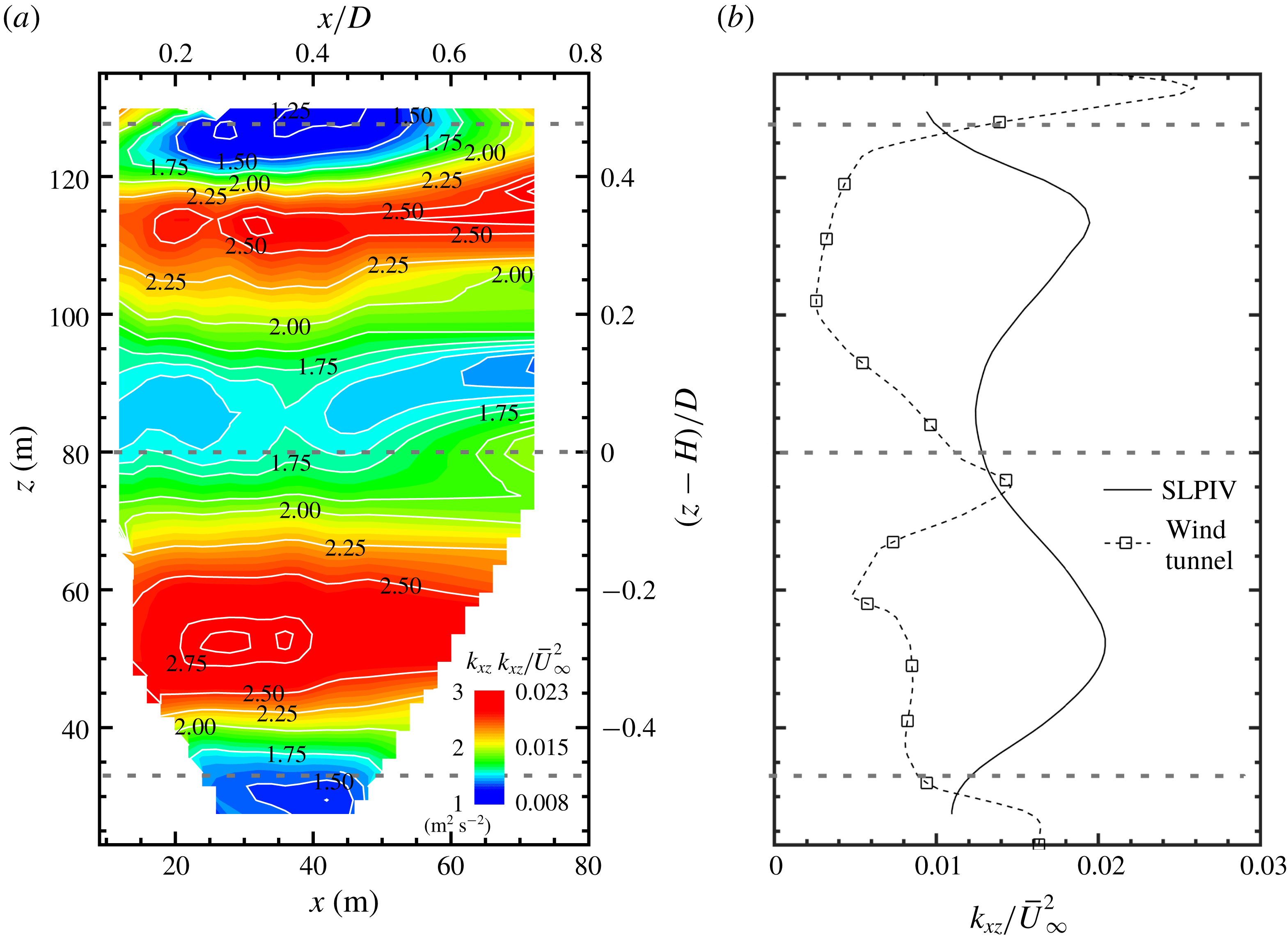
To examine the turbulent characteristics of the near wake, the in-plane turbulent kinetic energy (TKE, i.e.
 $k_{xz}=(\langle u^{\prime 2}\rangle +\langle w^{\prime 2}\rangle )/2$
, where
 $u^{\prime }$
and
 $w^{\prime }$
are the velocity fluctuations in
 $x$
and
 $z$
directions, respectively) is calculated using the instantaneous velocity fields and is presented in figure 5. The contour of
 $k_{xz}$
(figure 5
a) shows a region of relatively low
 $k_{xz}$
around the hub height, and local maxima of
 $k_{xz}$
in the region between the hub height and the elevations corresponding to the turbine blade tips. Quantitatively, a more than 80 % increase in
 $k_{xz}$
is observed in the region of local maxima with respect to the values in the region around the hub height. Accordingly, figure 5(b) presents the in-plane TKE profile extracted from the contour plot, in comparison to that from the wind tunnel experiment of Hancock & Pascheke (Reference Hancock and Pascheke2014). For better comparison, both profiles are scaled by
 $\overline{U}_{\infty }^{2}$
. Note that the lidar result of Iungo et al. (Reference Iungo, Wu and Porté-Agel2012) shown in figure 4 is not provided for TKE comparison here, since the paper only shows the TKE profiles along fixed elevation angles rather than at fixed streamwise locations, which makes the comparison difficult. As the figure shows, the
 $k_{xz}$
profile of SLPIV highlights a local minimum around the hub height. In contrast, the
 $k_{xz}$
profile from the wind tunnel measurement exhibits a strong upsurge, near the same region, around the blade root elevations. Such a difference is attributed to the spanwise offset of the two measurements. At the tower plane (i.e. in the case of the wind tunnel measurement), the turbulence associated with the nacelle wake can significantly enhance the near-wake TKE in this region. With a spanwise offset (i.e. in the case of the SLPIV measurement), the influence of nacelle wake on the local TKE decreases in the region around the hub height. In addition, the SLPIV result exhibits two local maximum values around
 $z=55~\text{m}$
and 112 m, respectively. The locations of the maxima correspond to
 $(z-H)/D\approx \pm 0.3$
, in the vicinity of the locations where ‘bumps’ in the velocity profiles are identified in figure 4(b), suggesting the
 $k_{xz}$
peaks may be connected to the high local mean velocity gradient. Such bumps are shifted to the region slightly outside of the blade tip at
 $(z-H)/D\approx \pm 0.55$
for the wind tunnel profile. Simple geometrical considerations reveal that the spanwise offset between measurement planes is insufficient to account for the difference observed in the figure. In other words, considering the TKE peaks above the hub height, peak in our measurement is below the corresponding elevation where the blade tip intersects the measurement plane, while in the wind tunnel measurement the TKE peak occurs above the blade tip elevation. Notably, a recent numerical study using LES on a model-scale turbine (Santoni et al.
Reference Santoni, Carrasquillo, Arenas-Navarro and Leonardi2017) revealed that a considerable (and asymmetrical) flux of TKE occurs in the spanwise directions. In addition, another LES study (Foti et al.
Reference Foti, Yang, Campagnolo, Maniaci and Sotiropoulos2018) showed that the operation region of the turbine also induces a shift of the TKE peaks (streamwise turbulence intensity in the paper, which is similar to TKE) to the inside of the blade tip elevations, specifically for region 3 of turbine operation. Therefore, we believe this shift of TKE peaks could be an effect of spanwise transport of TKE and/or variations in the region of operation of the turbine, which needs to be further investigated in future studies.
Before closing this section, it is worth pointing out that SLPIV can only resolve a certain percentage of the in-plane TKE due to the filtering effect associated with two-point cross-correlation with a finite interrogation window size. Correspondingly, the turbulence associated with flow structures smaller than our interrogation window, e.g. the velocity fluctuations induced within the snow voids formed by tip vortices, cannot be captured from our measurements. Hence, for the completeness of our analysis, a rough assessment of the filtering effect is provided here using sonic anemometer measurements which were shown to effectively capture wake turbulence, including that induced by the tip vortices at the EOLOS site (Toloui, Chamorro & Hong Reference Toloui, Chamorro and Hong2015). The assessment is conducted using the hub height sonic anemometer at the met tower for a time period of 14 min, different from that of the SLPIV experiment. The period is carefully selected using the following criteria: (i) mean wind direction of
 $-7^{\circ }$
from the north to ensure that the sonic anemometer is located inside the turbine wake but outside the influence zone of the wake of the met tower structure; (ii) mean wind speed of
 ${\sim}10~\text{m}~\text{s}^{-1}$
and a turbulence intensity of
 ${\sim}$
18 %, matching those of the SLPIV measurement. The in-plane TKE is calculated using both the filtered and unfiltered velocity components from the sonic anemometer data. Based on the Taylor frozen eddy hypothesis, the scale of the temporal filter is chosen to match the interrogation window size of the SLPIV measurements. Accordingly, the ratio of filtered to unfiltered in-plane TKEs is regarded as the percentage of the in-plane TKE captured by SLPIV. The result shows that SLPIV is capable of capturing 95 % of the total in-plane TKE. This estimate involves uncertainties due to the following reasons: (i) the sonic measurement provides only single-point estimates rather than those of the entire two-dimensional plane; (ii) the sonic and SLPIV measurements do not occur at the same period; (iii) the measurement location of SLPIV (centred around
 $x=0.41D$
) differs from that of the sonic anemometer (
 $x=1.71D$
). Note that the above analysis assumes the 20 Hz sonic anemometer captures all the TKE within the turbine wake. This assumption is reasonable since the energy-containing scale in the turbine wake has been shown to be close to (at least of the order of) that of atmospheric flows according to the literature (Vermeer et al.
Reference Vermeer, Sorensen and Crespo2003; Frandsen Reference Frandsen2007). According to Kunkel & Marusic (Reference Kunkel and Marusic2006), who compared the performance of hotwire and sonic anemometers for measuring atmospheric turbulence, we estimate the sonic anemometer captures
 ${>}97\,\%$
of TKE measured from the hot-wire under the field conditions of our SLPIV experiment.
To further investigate the characteristics of the near wake, the instantaneous velocity vector fields are examined individually in conjunction with the turbine operational conditions. In particular, figure 6 presents two samples of the instantaneous velocity field at different instances in time where the near wake depicts distinct behaviours, referred to as the wake expansion state and wake contraction state hereafter. Figures 6(a) and 6(b) show a sample of the instantaneous flow field and the corresponding streamwise velocity profile at
 $x=0.5D$
, respectively, illustrating a typical wake expansion state. The wake expansion, characterized by a significant velocity deficit in the central portion of the wake, is the dominant wake state as the turbine is operated to extract kinetic energy from the incoming wind. Nevertheless, it is observed that the near wake also exhibits contracting behaviour occasionally. As shown in figure 6(c,d), the wake contraction state exhibits a pronounced upsurge of the velocity in the central portion of the wake. In this region, the velocity magnitude rises above the average velocity (over the entire elevation span) of the wake, and occasionally exceeds the free stream velocity measured above the blade-top tip height in the field of view of the SLPIV.
Samples of instantaneous velocity field (
 $1:2$
skip applied in both horizontal and vertical directions for clarity) in the near wake of the EOLOS turbine showing two distinct wake behaviours. A sample of the wake expansion state including (a) the instantaneous velocity vector field superimposed with velocity magnitude contours and (b) the corresponding streamwise velocity profile at
 $x=0.5D$
. A sample of the wake contraction state including (c) the instantaneous velocity vector field superimposed with velocity magnitude contours and (d) the corresponding streamwise velocity profile at
 $x=0.5D$
.

A schematic illustrating inner and outer wake zones for the definition of wake velocity ratio
 $R_{w}$
.

To obtain a quantitative characterization of the two distinct wake states mentioned above, we introduce the wake velocity ratio
 $R_{w}$
based on the instantaneous near-wake velocity field obtained from SLPIV. Specifically, as shown in figure 7, the cross-section of the entire wake is divided into an inner disk (referred to as the inner wake hereafter) and an outer annulus (referred to as the outer wake hereafter) of equal area. Then
 $R_{w}$
is defined as the ratio of the spatially averaged velocity of the inner wake (
 $\bar{u}_{in}$
) to that of the outer wake (
 $\bar{u}_{out}$
), i.e.
 $R_{w}=\bar{u}_{in}/\bar{u}_{out}$
. At the sampling plane of the SLPIV (i.e.
 $y=0.19D$
), the inner wake corresponds to an elevation span from
 $z=46$
to 114 m, and the outer wake includes the region between
 $z=33$
and 46 m as well as that between
 $z=114$
and
 $z=127~\text{m}$
. For each instantaneous sample, we can calculate
 $\bar{u}_{in}$
and
 $\bar{u}_{out}$
by spatially averaging the streamwise velocity over the corresponding elevation spans within the field of view of the SLPIV, and subsequently obtain the
 $R_{w}$
. Note that the streamwise velocity of the entire region rather than that at a specific streamwise location is used for spatial averaging to ensure a more robust characterization of the inner wake flow speed in comparison to that of the outer wake. According to the definition of
 $R_{w}$
,
 $R_{w}>1$
indicates the averaged streamwise velocity in the inner wake is higher than that in the outer wake, representing the characteristic of a wake contraction, while
 $R_{w}<1$
suggests a lower velocity in the inner wake and matches the trait of wake expansion. In the following analysis, the
 $R_{w}$
will be employed to quantify the different wake states. Nevertheless, it is important to point out that the contraction state defined using
 $R_{w}>1$
does not necessarily correspond to a propeller state of a wind turbine which would require a comparison between the incoming and the wake flows. Instead, the
 $R_{w}$
criterion provides a demarcation of when the turbine operates at the desired conditions and when it is underperforming, which leads to a reduced velocity deficit in the inner wake.
(a) Time series of wake ratio
 $R_{w}$
. (b) Probability histogram of
 $R_{w}$
.

Figure 8(a) shows the variation of
 $R_{w}$
over the time duration of the SLPIV measurements. In this period, the turbine was operated mostly in the region
 ${>}$
2 (i.e. 94.6 % of the time) and the averaged yaw error was
 $5.42^{\circ }$
. The mean value of
 $R_{w}$
was
 $\langle R_{w}\rangle =0.947$
, indicating a predominately wake expansion state according to our
 $R_{w}$
-criterion described above. However, the
 $R_{w}$
also fluctuates substantially over the period and has a standard deviation,
 $\unicode[STIX]{x1D70E}_{R_{w}}=0.089$
. Particularly, approximately 25 % of the time duration can be classified as a wake contraction state with
 $R_{w}>1$
. Moreover, figure 8(b) indicates approximately 16 % of the time duration yields a value of
 $R_{w}$
that is more than one
 $\unicode[STIX]{x1D70E}_{R_{w}}$
above
 $\langle R_{w}\rangle$
, representing a strong wake contraction state, while approximately 10 % of the cases have
 $R_{w}$
more than one
 $\unicode[STIX]{x1D70E}_{R_{w}}$
below
 $\langle R_{w}\rangle$
which is classified as a strong expansion for the following analysis.
Schematics illustrating the blade element velocities and the corresponding angles associated with blade element velocity triangle.

Although not discussed extensively in the literature, the variation of wake states observed here is reminiscent of the wind turbine wake transition to a propeller state reported in a number of prior analytical and numerical studies (Eggleston & Stoddard Reference Eggleston and Stoddard1987; Sørensen, Shen & Munduate Reference Sørensen, Shen and Munduate1998; Sebastian & Lackner Reference Sebastian and Lackner2011, Reference Sebastian and Lackner2012). These studies suggest that wind turbine wakes can show a contraction-like behaviour under specific conditions of operation. Specifically, the theoretical analysis presented in Eggleston & Stoddard (Reference Eggleston and Stoddard1987) pointed out that wake contraction phenomena can appear in the operation of a variable-pitch turbine with an axial induction factor (
 $a$
) greater than 0.5. They referred to the operating state of the turbine under such conditions as the propeller transition state, including turbulent wake state (TWS) occurring for
 $0.5<a<1.0$
and the vortex ring state (VRS) occurring for thrust coefficient,
 $C_{T}>1.0$
and
 $a>1.0$
(figure 2.7 on page 32 of Eggleston & Stoddard (Reference Eggleston and Stoddard1987)). They further showed that the specific values of
 $C_{T}$
and
 $a$
causing different turbine operational states depend on the relative values of blade pitch (
 $\unicode[STIX]{x1D6FD}$
) and relative velocity angle (
 $\unicode[STIX]{x1D6F7}$
) formed at the wind turbine blade leading edge, as illustrated in figure 9. During regular operation, the turbine is continuously subjected to highly fluctuating incoming velocities
 $U_{\infty }$
, due to atmospheric turbulence, and rapid
 $\unicode[STIX]{x1D6FD}$
changes associated with the turbine control mechanism. The net effect of such rapid changes is a change in the angle of attack
 $\unicode[STIX]{x1D6FC}$
shown in figure 9(c). The results from this theoretical work were supported by a follow-up study from Sørensen et al. (Reference Sørensen, Shen and Munduate1998) using a numerical method that combines the actuator disc principle with the Navier–Stokes equations, which provided additional refinement of the transition conditions of different turbine wake states. The specific role of unsteady effects was further explored by Sebastian & Lackner (Reference Sebastian and Lackner2011, Reference Sebastian and Lackner2012) who studied the appearance of propeller transition states for the case of offshore turbines subjected to highly unsteady conditions (e.g. turbines undergoing rocking motion due to turbine tower/platform pitching). Specifically, these transition states, which essentially cause the wake to contract, representing a momentary loss of lift of the turbine, were correlated to the time derivative of the pitch of the turbine tower. Exclusively during leeward motion, the turbine blade bound circulation was found to change from a positive to a negative value indicating a clear transition to propeller states. As the turbine tower moves in the leeward direction, the relative velocity of the incoming wind approaching the blade decreases (i.e. decrease of the angle of attack) which causes a loss of lift. Alternatively, as
 $U_{\infty }$
drops suddenly (resulting in a much lower
 $\unicode[STIX]{x1D6FC}$
) due to any other unsteadiness, the wind turbine may not extract any energy at that moment and instead acts like a propeller as the rotor cannot slow down rapidly due to inertia. In addition, the turbine tower in leeward motion can cause the rotor to interact with its own wake which also contributes to the contraction of the turbine wake (Sebastian & Lackner Reference Sebastian and Lackner2011). It is noteworthy that, using numerical simulation, Sebastian & Lackner (Reference Sebastian and Lackner2011) also showed that propeller transition states occur a staggering 30 %–50 % of the time for offshore (floating and monopile) turbines. Specifically, the monopile type of offshore turbines, which are similar to on-land turbines in the way they are mounted, do undergo wake transitions approximately 30 % of the time, which is close to the observations in the current SLPIV study.
Following guidance from the above-mentioned literature, we examined blade pitch (
 $\unicode[STIX]{x1D6FD}$
), incoming velocity (
 $U_{\infty }$
), the effective angle of attack (
 $\unicode[STIX]{x1D6FC}_{E}$
), revolutions per minute (r.p.m.) of the rotor (
 $\unicode[STIX]{x1D6FA}$
),
 $\unicode[STIX]{x1D6F7}$
and the gradient of blade pitch (
 $\text{d}\unicode[STIX]{x1D6FD}/\text{d}t$
) to study the wake expansion and contraction states (defined using
 $R_{w}$
-criterion). Two key turbine operational parameters that represent the relative positioning of the turbine blades and the wind are the effective angle of attack
 $\unicode[STIX]{x1D6FC}_{E}$
and the blade pitch
 $\unicode[STIX]{x1D6FD}$
. Both parameters are readily available from the sensor readings of the EOLOS turbine. The former is derived using
 $\unicode[STIX]{x1D6FC}_{E}=a\tan (2U_{\infty }(1-a)/\unicode[STIX]{x1D6FA}D(1+a))-\unicode[STIX]{x1D6FD}-\unicode[STIX]{x1D6FD}_{0}$
, where
 $U_{\infty }$
is measured from the sonic anemometer on the nacelle,
 $\unicode[STIX]{x1D6FA}$
is the turbine rotational speed,
 $D$
is the rotor diameter,
 $\unicode[STIX]{x1D6FD}$
is the blade pitch angle controlled by the control mechanism and
 $\unicode[STIX]{x1D6FD}_{0}$
is the blade pre-twist of
 $2.1^{\circ }$
, and the axial induction factor
 $a$
is neglected in the calculation of
 $\unicode[STIX]{x1D6FC}_{E}$
due to the relatively large uncertainty involved in its estimate. Here
 $U_{\infty }$
is estimated at the hub height which does not capture the variation of local wind speed approaching the turbine blades across the entire rotor span. Therefore, the latter (
 $\unicode[STIX]{x1D6FD}$
) is introduced potentially as a more effective indicator of change of blade position relative to the wind since it is controlled by the pitch control unit at nacelle and is not affected by the variation of incoming wind speed across the rotor span.
Figure 10 presents histograms of wake states over the effective angle of attack (i.e.
 $\unicode[STIX]{x1D6FC}_{E}$
) and the rate of change of blade pitch (i.e.
 $\text{d}\unicode[STIX]{x1D6FD}/\text{d}t$
). To reduce the adverse impact of a number of uncertainties on the correlation among wake states and these turbine operational parameters, the following pre-processing steps have been applied to the data before they are presented in figure 10. First, a 10 s low-pass filter is applied to
 $\unicode[STIX]{x1D6FC}_{E}$
to eliminate the jitter in the signal. The 10 s span is determined considering that
 $\unicode[STIX]{x1D6FC}_{E}$
is employed to represent the relative positioning of the turbine blades and the wind across the entire rotor span in an average sense. With a rotor diameter of 96 m and the averaged incoming wind velocity measured at the hub height of
 ${\sim}10~\text{m}~\text{s}^{-1}$
, the turbulent flow time scale corresponding to the spatial scale of the rotor span is approximately 10 s based on the Taylor frozen eddy hypothesis. In general, this low-pass filter reduces the impact of the uncertainties associated with the variation of flow speed across the rotor span in our analysis. For consistency, the blade pitch and the
 $R_{w}$
are also smoothed with the low-pass filter of the same size. In addition, for better correlation between wake flows and turbine operation, a 4 s shift (backward in time) is applied to the data of
 $R_{w}$
considering the difference of locations between the rotor plane and the centre of the SLPIV measurement region as well as the average wind speed at the hub height. Moreover, conditional sampling is employed on the turbine operation region (i.e. region
 ${>}$
2 to rule out time periods with a constant blade pitch of
 $1^{\circ }$
). This condition ensures only time periods with varying
 $\unicode[STIX]{x1D6FD}$
are considered to calculate
 $\text{d}\unicode[STIX]{x1D6FD}/\text{d}t$
. As a last step, conditional sampling on nacelle misalignment (i.e. the misalignment angle between the rotor axis and the light sheet orientation) is also applied to avoid the influence of the nacelle flow structures on the FOV. Both conditional sampling steps in total eliminated
 ${\sim}$
23 % of the data samples over the SLPIV measurement duration of 1790 s (
 ${\sim}$
30 min).
Probability histograms of
 $\unicode[STIX]{x1D6FC}_{E}$
and
 $\text{d}\unicode[STIX]{x1D6FD}/\text{d}t$
under different
 $R_{w}$
ranges.
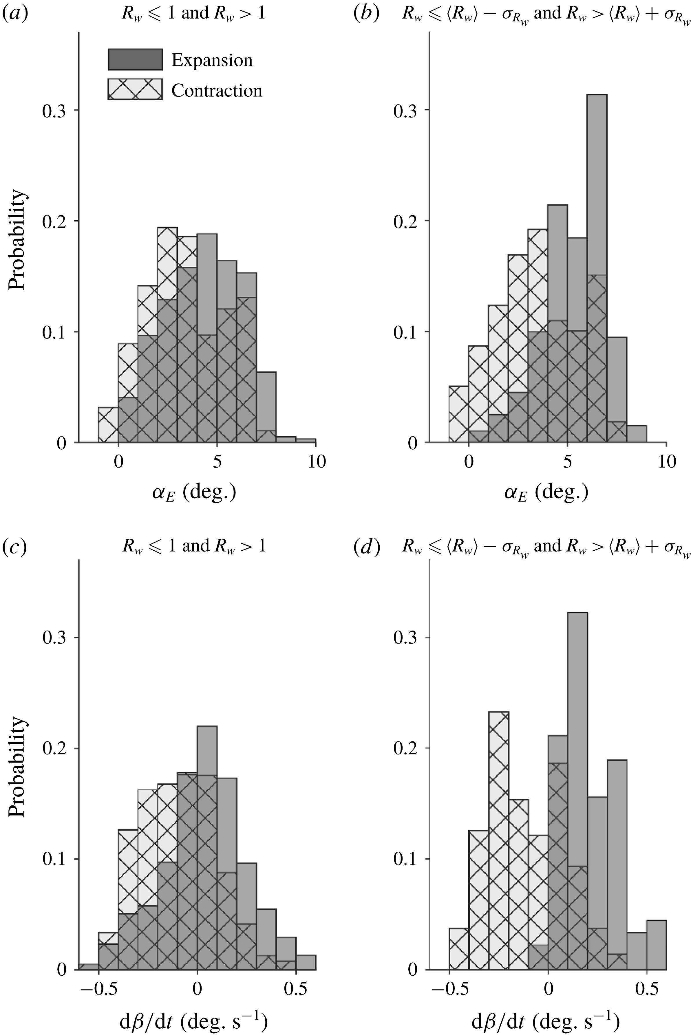
As shown in figure 10(a), the histograms of the wake expansion and contraction states do not show any appreciable separation over
 $\unicode[STIX]{x1D6FC}_{E}$
when all expansion and contraction events are considered (i.e.
 $R_{w}<1$
for expansion and
 $R_{w}>1$
for contraction). Nevertheless, a remarkable shift of the histogram for the contraction state towards negative
 $\unicode[STIX]{x1D6FC}_{E}$
can be observed when only strong expansion and contraction events (i.e.
 $R_{w}\leqslant \langle R_{w}\rangle -\unicode[STIX]{x1D70E}_{R_{w}}$
for expansion and
 $R_{w}>\langle R_{w}\rangle +\unicode[STIX]{x1D70E}_{R_{w}}$
for contraction) are included (figure 10
b). Compared to the trend for
 $\unicode[STIX]{x1D6FC}_{E}$
, the expansion and contraction histograms exhibit a significantly clearer separation over
 $\text{d}\unicode[STIX]{x1D6FD}/\text{d}t$
(figure 10
c,d). In particular, the mean value of
 $\text{d}\unicode[STIX]{x1D6FD}/\text{d}t$
for expansion and contraction is
 $0.21~\text{deg}~\text{s}^{-1}$
and
 $-0.11~\text{deg}~\text{s}^{-1}$
(figure 10
c), respectively. When only strong expansion and contraction events are sampled (figure 10
d), 98 % of strong expansion events occur at positive
 $\text{d}\unicode[STIX]{x1D6FD}/\text{d}t$
and 67 % of strong contraction is concentrated in the region of negative
 $\text{d}\unicode[STIX]{x1D6FD}/\text{d}t$
. Overall, figure 10 clearly shows a strong connection between the wake states and turbine operational parameters. Compared to
 $\unicode[STIX]{x1D6FC}_{E}$
,
 $\text{d}\unicode[STIX]{x1D6FD}/\text{d}t$
is evidently the more effective parameter to correlate with the transition of wake states owing to the uncertainties involved in the estimation of
 $\unicode[STIX]{x1D6FC}_{E}$
using the available sensor information from the turbine.
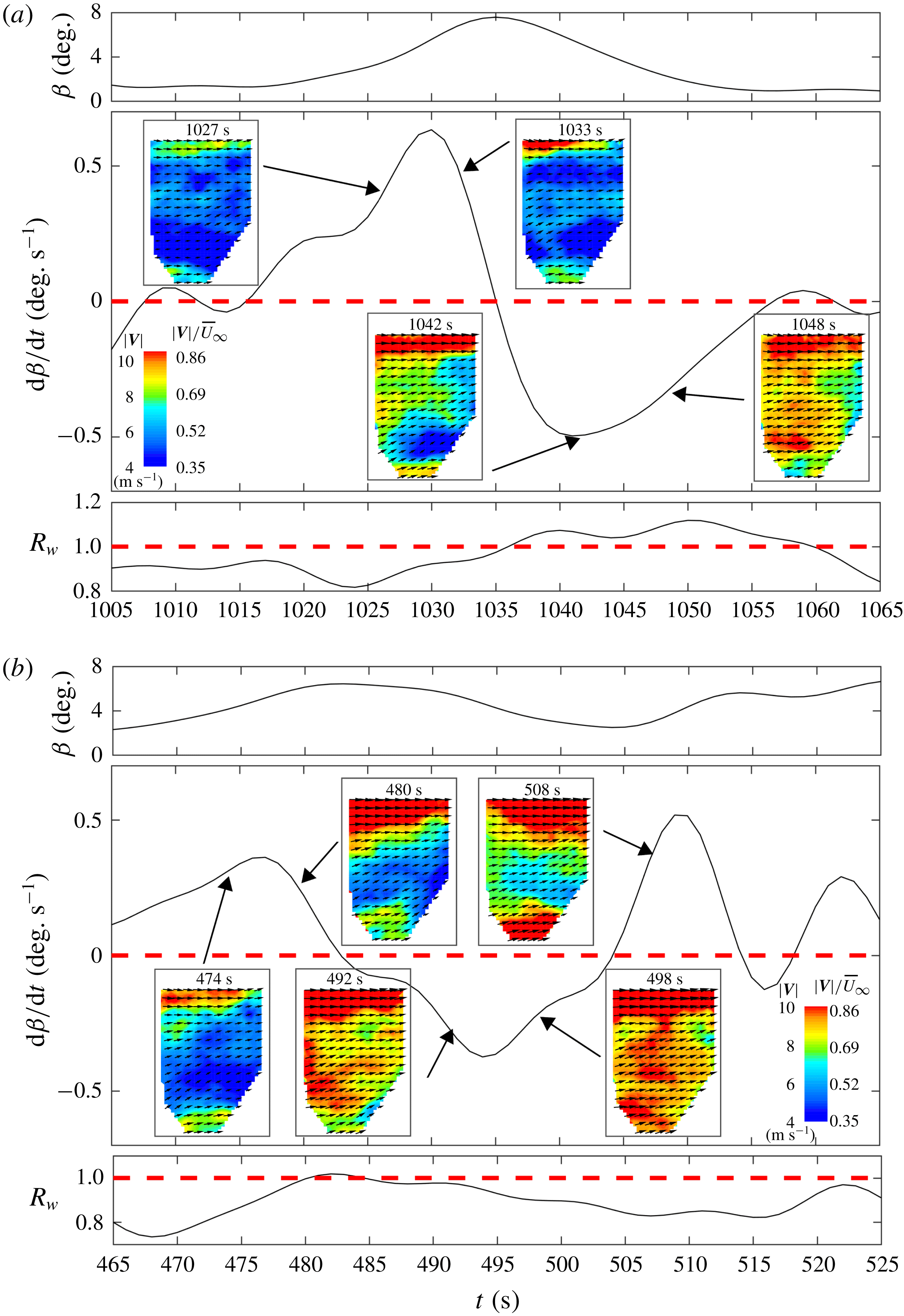
To further substantiate the direct connection between the pitch control and the wake transition, two sample time sequences of
 $R_{w}$
are extracted from SLPIV. Each sequence has a time duration of 60 s, covering at least one incident of the wake transition between wake expansion and contraction states. The sequences of
 $R_{w}$
, corresponding
 $\unicode[STIX]{x1D6FD}$
and
 $\text{d}\unicode[STIX]{x1D6FD}/\text{d}t$
(with low-pass filter applied as mentioned in the last paragraph) are presented in figure 11. The SLPIV velocity fields corresponding to these two time sequences are provided as supplementary movies 1 and 2 available at https://doi.org/10.1017/jfm.2018.779. Figure 11(a) shows a sequence that consists of a strong wake contraction event, in which
 $R_{w}$
becomes significantly larger than 1 for
 ${\sim}$
40 % (23 s out of 60 s) of the entire time duration. The figure shows a clear one-to-one correspondence between
 $R_{w}$
and
 $\text{d}\unicode[STIX]{x1D6FD}/\text{d}t$
. Specifically, as
 $\unicode[STIX]{x1D6FD}$
increases during the time stamps of 1015–1035 s,
 $\text{d}\unicode[STIX]{x1D6FD}/\text{d}t$
is positive and the corresponding
 $R_{w}<1$
. Accordingly, in this period, the wake flow stays predominantly in the expansion state (evidenced by the two inset figures at 1027 and 1033 s; please see the supplementary movie 1 for more information). As soon as
 $\unicode[STIX]{x1D6FD}$
starts decreasing at approximately 1035 s,
 $\text{d}\unicode[STIX]{x1D6FD}/\text{d}t$
becomes negative and
 $R_{w}$
rises above 1 within
 $\pm 1~\text{s}$
(i.e. within the uncertainty involved in the time shift between the rotor plane and the centre of the SLPIV measurements). The corresponding wake flow switches to the contraction state and shows consistent contraction until approximately 1060 s when
 $\text{d}\unicode[STIX]{x1D6FD}/\text{d}t$
goes back to approximately 0 and
 $R_{w}$
drops to values very close to 1 (evidenced by the two inset figures at 1042 and 1048 s; and check the supplementary movie 1 for viewing the dynamic process of wake transition). For comparison, as shown in figure 11(b), the second time sequence is selected to show the wake transition that involves a weak contraction/expansion event (i.e. with
 $R_{w}$
in the close vicinity of 1). Similar to figure 11(a), the correspondence between
 $\text{d}\unicode[STIX]{x1D6FD}/\text{d}t$
and
 $R_{w}$
is still appreciable. Specifically,
 $\text{d}\unicode[STIX]{x1D6FD}/\text{d}t$
starts with a positive value, then drops below 0 and rises above 0, while accordingly,
 $R_{w}$
increases from significantly below 1 to slightly above 1 and drops down. However, as shown in the corresponding inset figures of the wake velocity fields and the supplementary movie 2, the absolute value of
 $R_{w}$
is not a clear indicator of a contraction/expansion wake state. This situation corresponds to the distributions in the vicinity of
 $\text{d}\unicode[STIX]{x1D6FD}/\text{d}t=0$
in figure 10(d), where there is no substantial separation between the wake expansion and contraction states over
 $\text{d}\unicode[STIX]{x1D6FD}/\text{d}t$
. Such a situation occurs when the flow surge in the inner wake introduced by negative
 $\text{d}\unicode[STIX]{x1D6FD}/\text{d}t$
is not strong enough compared to the outer wake velocity, and the turbine performance is less affected.
Sample time sequences of the blade pitch
 $\unicode[STIX]{x1D6FD}$
, the corresponding rate of change of pitch
 $\text{d}\unicode[STIX]{x1D6FD}/\text{d}t$
and
 $R_{w}$
showing the wake transition involving (a) a strong contraction state and (b) a weak contraction state. Inset figures are the instantaneous velocity vector fields (
 $1:3$
skip applied in both horizontal and vertical directions for clarity) superimposed with the velocity magnitude contours obtained from SLPIV measurements.
To summarize, the above analysis indicates that the temporal variation in
 $\unicode[STIX]{x1D6FD}$
(i.e.
 $\text{d}\unicode[STIX]{x1D6FD}/\text{d}t$
) is best correlated with the contraction phenomena identified through
 $R_{w}$
. Furthermore, to establish a physical link between
 $\text{d}\unicode[STIX]{x1D6FD}/\text{d}t$
and turbine (both tower and blade) deflection as suggested in the literature (e.g. Sebastian & Lackner (Reference Sebastian and Lackner2011)), we analyse the signals of tower strain and blade strain gauges installed on the EOLOS turbine during our flow measurements. Figure 12 presents the signals of these strain gauges together with the blade pitch change, illustrating the strong connections between the
 $\unicode[STIX]{x1D6FD}$
variations and the thrust on the turbine tower and blades. Specifically, figure 12(a) shows a strong negative correlation with a correlation coefficient of
 $-$
0.90 between the blade pitch and the tower foundation strain measured on the downstream side of the turbine (a measure of leeward motion of the turbine). Similarly, a strong correlation (correlation coefficient of
 $-$
0.92) is found between the blade pitch variations and the flapwise deflections of the rotor measured by the blade strain gauges mounted at 44.4 % span of the blade (21.6 m from the blade root, i.e. the farthest point where a strain gauge is installed) on the high pressure side as shown in figure 12(b). The results suggest that as
 $\unicode[STIX]{x1D6FD}$
decreases, both the blades and the tower are flexed in the leeward direction (into the rotor wake), causing interaction between the rotor and the turbine wake that results in wake contraction, as identified in the above-mentioned literature and observed in our experiments.
Time series of (a) blade pitch
 $\unicode[STIX]{x1D6FD}$
(solid line) and tower strain (dashed line) representing tower deflections in the streamwise direction of the flow, and (b) blade pitch
 $\unicode[STIX]{x1D6FD}$
(solid line) and the blade strain (dashed line) representing flapwise deflection from high pressure side to the low pressure side. Both strains are reported in microstrain.

It is to be noted that on-land turbines may not have the intense rocking motion expected for offshore turbines, but the literature has provided support for substantial deflection of the tower and blades experienced by utility-scale on-land turbines, particularly during higher regions of operation. For the tower deflection, Bang, Kim & Lee (Reference Bang, Kim and Lee2012) performed measurements on a 1.5 MW turbine and found that the turbine tower deflects by 0.17 m at the nacelle elevation during the low wind conditions. Nasrabad (Reference Nasrabad2016) carried out FAST simulations on 1.5 MW turbine and showed that the turbine nacelle could deflect by 0.2 m under normal operation. Another recent study, by Zendehbad, Chokani & Abhari (Reference Zendehbad, Chokani and Abhari2017), conducted experiments on a 2 MW turbine using a novel ground-based optical technique and demonstrated a strong correlation between the tower tip deflection and the strain gauge measurements at the tower foundation. The study also revealed the turbine tower to deflect by a maximum of 0.8 m for high wind velocities (which are very similar to our experimental conditions). Although the experiments measured deflections of the tower in the sideways direction (perpendicular to the incoming wind direction), the study highlights the extent of the deflections that typical on-land turbines experience. Moreover, through accelerometer measurements conducted on a 3 MW offshore turbine, El-kafafy et al. (Reference El-kafafy, Devriendt, Weijtjens, Sitter and Necati2014) showed that the deflections in the predominant wind direction (fore–aft direction), which constitute a primary mode of vibration, are typically 50 % higher than that those in the sideways direction. For turbine blade deflection, using FAST simulations on NREL 5 MW (126 m diameter rotor, 90 m hub height) turbine, Jonkman et al. (Reference Jonkman, Butterfield, Musial and Scott2009) showed that the turbine blades experience a 10 times larger deflection in the fore–aft direction (4–5.5 m relative to the undeflected blade pitch axis) compared to a typical nacelle deflection of 0.5 m in the fore–aft direction when the turbine operates above region 2. Follow-up numerical simulations on utility-scale turbines based on fluid–structure interaction, by Bazilevs et al. (Reference Bazilevs, Hsu, Kiendl, Wüchner and Bletzinger2011) and Bazilevs et al. (Reference Bazilevs, Takizawa, Tezduyar, Hsu, Kostov and McIntyre2014), further found flapwise deflections of up to 5.6 m.
Schematic illustrating the fore–aft deflection of the turbine tower and the blade flapwise deflection due to blade pitch (
 $\unicode[STIX]{x1D6FD}$
) variation. (a) Typical wake expansion state of the turbine and (b) wake contraction state caused by the interaction of rotor and turbine wake.

Overall, based on the above-mentioned literature and the strong correlations between blade pitch and the thrust forces on the tower and blades observed in our experiments, we suggest that the interaction between rotor and turbine wake can contribute considerably to the wake contraction. This mechanism is schematically represented in figure 13. As blade pitch
 $\unicode[STIX]{x1D6FD}$
decreases, the turbine tower and blades flex in the streamwise direction, as shown in figure 13(b), leading to wake contraction. We also acknowledge that aeroelastic flutter of the turbine blades, during rapid changes of
 $\unicode[STIX]{x1D6FC}$
or rocking of the turbine, could also play a role in the appearance of wake transitions, though it is not considered in the current analysis. It is noteworthy that, to the best of our knowledge, very few laboratory and field experiments have reported and discussed such intermittent wake transition, which may be attributed to the following reasons. Regarding the laboratory experiments, the incoming flow conditions are generally idealized and the turbine models do not fully capture the control dynamics and mechanical characteristics of utility-scale turbines. For field measurements, the conventional techniques do not have sufficient temporal and spatial resolution to capture such wake behaviour. In addition, the majority of field measurements were conducted further downstream of the turbines where such intermittent wake behaviour may not persist.
3.2 Near-wake tip vortex behaviours
In this section, the behaviours of near-wake tip vortices visualized as snow voids are analysed and correlated with turbine operation/response parameters. This analysis is an extension of the work from Hong et al. (Reference Hong, Toloui, Chamorro, Guala, Howard, Riley, Tucker and Sotiropoulos2014) which, for the first time, demonstrated the inter-connection between tip vortex behaviour and turbine operation/response parameters using a 6 min video of snow voids in the near wake of a utility-scale turbine. As described in § 2, the present analysis includes 4 datasets (i.e. Apr 2014, Nov 2015, Dec 2015, Feb 2016a) with a total duration of 2 h and with a field of view confined to the region covering the tip vortices generated at the blade-bottom tip level. These datasets, obtained from multiple deployments conducted in 2014–2016, cover a wide range of turbine operational and atmospheric conditions. The turbine operation/response parameters used for the analysis include critical turbine supervisory control and data acquisition (SCADA) parameters, their derivatives as well as the strain sensor data at the base of the turbine tower. These parameters either have been employed or can be readily incorporated into the control strategy of the turbine. As discussed in § 1, the behaviour of tip vortices in the near wake can significantly influence the turbulence characteristics and the evolution of the wake far downstream. Therefore, the analysis in the section aims to establish a statistical correlation between tip vortex behaviour and readily available operational and response information from utility-scale turbines, which can benefit wind energy developers in formulating advanced control strategies to improve the total power production and load mitigation of wind farms in the future.
In the present analysis, the tip vortex behaviour is categorized primarily into a consistent state and disturbed state, according to the general temporal variation of snow void patterns shown in each image frame of the recorded videos. The disturbed state is further divided into different types, referred to as Type I, Type II and Type III hereafter, based on specific features of the disturbed snow voids in the images. Figure 14 presents sample images illustrating the consistent state of tip vortices and different types of disturbed state. As figure 14(a) shows, the consistent state of tip vortices is characterized by a sequence of snow voids with clearly defined outlines, typically resembling the shape of a disk or an ellipse with a tapered tail. The number of voids appearing in the images ranges from 3 to 5 in our datasets, depending on the incoming flow velocity and tip-speed-ratio of the turbine. In the Type I disturbed state, as shown in figure 14(b), the snow voids are utterly unrecognizable or absent within the field of view. In contrast, for both Type II (figure 14
c) and III (figure 14
d) disturbed states, snow voids are still identifiable but smeared due to disturbance. Particularly, Type III state shows disturbed voids associated with vortex interactions such as leap frogging (i.e. roll-up of adjacent tip vortex filaments around each other) and merging, while such vortex interactions are not appreciable in the Type II state. To obtain an objective classification of different tip vortex states, we use the criteria based on the temporal variation of void size, void shape and void spacing for the first void (i.e. the most upstream void which is expected to be best correlated with the turbine operation) that enters the field of view of our measurements. These criteria are summarized in table 3. Specifically, tip vortex voids are earmarked as consistent only if all of the criteria are satisfied and as Type II/III if at least one criterion is satisfied. In addition, based on these criteria, we have developed image analysis algorithms to autonomously classify different vortex states. The results from the autonomous image processing are not very sensitive to the change of the exact threshold (i.e. 50 % in the table) within the range of 50 %–80 %. Note that although we present the qualitative observation of Type II and III disturbed states as mentioned above, we do not differentiate the two states through quantitative metrics due to the challenges of determining non-ambiguous metrics for such classification. More importantly, as the classification of the void states is mutually exclusive, a robust decorrelation of the samples is ensured. The decorrelation process renders
 $2/3$
of the total duration of the visualization data for correlating with turbine operation/response, i.e. for example, the Feb 2016a dataset which is 1790 s long produces 1193 tip vortex behavioural events/classifications which are completely de-correlated from one another.
Sample images of snow voids illustrating (a) consistent state, (b) Type I disturbed state, (c) Type II disturbed state and (d) Type III disturbed state of tip vortices.

The criteria used to classify different tip vortex states.

In the following analysis, the probabilistic distribution of turbine operation/response parameters corresponding to the categorized tip vortex states above is examined in the form of histograms. For this statistical analysis, we have conducted a thorough exploration of the information available in the EOLOS turbine database at the time duration corresponding to the tip vortex videos. Such information includes: (i) turbine SCADA parameters such as wind velocity measured from the sonic anemometer at the nacelle (used for gauging turbine tip-speed-ratio and controlling turbine operational region and yaw angle), turbine power, rotor speed and blade pitch; (ii) the strain gauge data at the turbine tower base. Several critical variables are also derived from turbine operation/response, namely, normalized turbine power
 $P^{\ast }$
and downwind tower strain
 $S^{\ast }$
, the corresponding fluctuation intensity of power
 $I_{P}$
, fluctuation intensity of tower strain
 $I_{S}$
and effective angle of attack
 $\unicode[STIX]{x1D6FC}_{E}$
. All these variables are used for a statistical demarcation of consistent and disturbed states of tip vortices and are presented in the analysis below. Specifically, the normalized turbine power
 $P^{\ast }$
is calculated as
 $(P-P_{min})/(P_{max}-P_{min})$
where
 $P$
,
 $P_{min}$
and
 $P_{max}$
are the instantaneous, minimum and maximum values of power recorded within a dataset, respectively, and the downwind tower strain
 $S^{\ast }$
is obtained through the same fashion of normalization as that of the power, with the data from the strain gauge closest to the direction opposite (i.e.
 $180^{\circ }$
) to the mean wind direction of each dataset. The fluctuation intensity of power
 $I_{P}$
is calculated as the ratio of standard deviation of the power
 $P$
to the mean of
 $P$
over a sliding period of 30 s. The fluctuation intensity of strain
 $I_{S}$
is calculated in the same fashion as that of
 $I_{P}$
. The effective angle of attack
 $\unicode[STIX]{x1D6FC}_{E}$
is derived following the same method as in § 3.1. In addition, considering the highly unsteady and multivariate nature of field measurements, a conditional sampling technique is applied in the current analysis to: (i) improve statistical demarcation of tip vortex behaviours with turbine operation/response parameters; (ii) elucidate underlying physical mechanisms governing turbine operational condition and tip vortex behaviours. Particularly, for the present analysis, the turbine yaw error (i.e. the misalignment angle between the wind direction and the rotor axis), turbine operational regions and types of disturbed tip vortex state are chosen as conditional sampling parameters.
The probability histograms of power fluctuation intensity (
 $I_{P}$
), tower strain fluctuation intensity (
 $I_{S}$
) and effective angle of attack (
 $\unicode[STIX]{x1D6FC}_{E}$
) for consistent and disturbed states of tip vortices under no yaw error restriction (a–c) and a restriction of yaw error
 ${<}3^{\circ }$
(d–f).

Figure 15 presents the probability histograms of power fluctuation intensity
 $I_{P}$
, tower strain fluctuation intensity
 $I_{S}$
and effective angle of attack
 $\unicode[STIX]{x1D6FC}_{E}$
for consistent and disturbed states of tip vortex events under different restrictions of yaw error. Specifically, no yaw error restriction is applied in figure 15(a–c) while a stringent restriction of yaw error
 ${<}3^{\circ }$
is employed in figure 15(d–f). For each histogram, twelve bins of equal size, covering from the minimum to maximum values of each turbine operation/response variable presented in the histogram, are selected to demonstrate the statistical distribution of the turbine variables under consistent and disturbed tip vortex states. A similar convention of bin size choice is employed consistently throughout the paper. Without a yaw error restriction, no significant difference in the
 $I_{P}$
histogram between the consistent and disturbed states (figure 15
a) is observed. However, there is a clear separation in the distribution of
 $I_{S}$
for consistent and disturbed states of tip vortices (figure 15
b). For the disturbed state, the distribution of
 $I_{S}$
appears to follow a normal distribution, while a significant portion of
 $I_{S}$
is clearly biased towards the lower values of
 $I_{S}$
for the consistent state. With an increased yaw error restriction, there is an improved separation of the
 $I_{S}$
histograms between consistent and disturbed states of the tip vortices, as shown by a comparison of figures 15(b) and 15(e). In particular, with increasing yaw restriction, the
 $I_{S}$
histogram of the consistent state approaches an exponential distribution, characterized as
 $0.62\text{e}^{-14.87I_{s}}$
through least square fitting. It is worth noting that an exponential distribution was identified for the relationship between the tip vortex stability and the turbulence intensity of the incoming flow in recent wind turbine LES studies (e.g. Ivanell et al. (Reference Ivanell, Mikkelsen, Sørensen and Henningson2010) and Sarmast et al. (Reference Sarmast, Dadfar, Mikkelsen, Schlatter, Ivanell, Sørensen and Henningson2014)), which may shed some light on the underlying mechanism of the trend observed for
 $I_{S}$
here. As a comparison, with an increasing yaw restriction, the
 $I_{S}$
histogram of the disturbed state resembles a normal distribution with the mean value moving towards higher
 $I_{S}$
. The least square fit of the histogram yields a normal distribution with a mean value of 0.13 and a standard deviation of 0.06. In contrast to the
 $I_{S}$
histograms, the
 $I_{P}$
histograms (figure 15
a,d) and
 $\unicode[STIX]{x1D6FC}_{E}$
histograms (figure 15
c,f) do not seem to be strongly affected by the yaw error restriction. Similarly, the normalized turbine power
 $P^{\ast }$
and tower strain
 $S^{\ast }$
are not appreciably influenced by the yaw error restriction, and therefore are not shown in figure 15 for brevity. To summarize here, figure 15 suggests a correlation between the tip vortex behaviour and tower strain fluctuations which represent fluctuations in the inherent strength of the vortices. In addition, these trends improved with yaw error restriction, indicating a definite effect of wind direction misalignment which needs to be minimized for further investigation. Therefore, for the following analysis in this paper, the yaw error is restricted to be less than
 $3^{\circ }$
, consistent with the restriction imposed in figure 15(d–f).
To further elucidate the correlations between the tip vortex behaviour and the turbine operation/response parameters, a restriction on the regions of turbine operation is applied to the analysis to de-couple the effects caused by the turbine control unit (TCU) operation, and results are presented in figure 16. Figure 16(a–e) shows histograms when the turbine operates in region 2 or below, during which TCU is designed to maximize power extraction with the available sub-optimal wind speeds by setting blade pitch to the minimum. For comparison, figure 16(f–i) presents histograms for regions greater than 2, where the turbine operation is regulated to maintain a relatively constant output power and the rotational speed of the turbine blades to protect the turbine from overload and structural failure. According to the changing TCU operation, the distributions of the consistent and disturbed states of the tip vortices as functions of turbine operation/response parameters vary substantially, as shown in the figure.
The probability histograms of power fluctuation intensity (
 $I_{P}$
), tower strain fluctuation intensity (
 $I_{S}$
), effective angle of attack (
 $\unicode[STIX]{x1D6FC}_{E}$
), turbine power (
 $P^{\ast }$
) and tower strain (
 $S^{\ast }$
) for consistent and disturbed tip vortex states under a restriction of yaw error
 ${<}3^{\circ }$
for (a–e) turbine operational regions
 ${\leqslant}2$
and (f–j) turbine operational regions
 ${>}2$
.
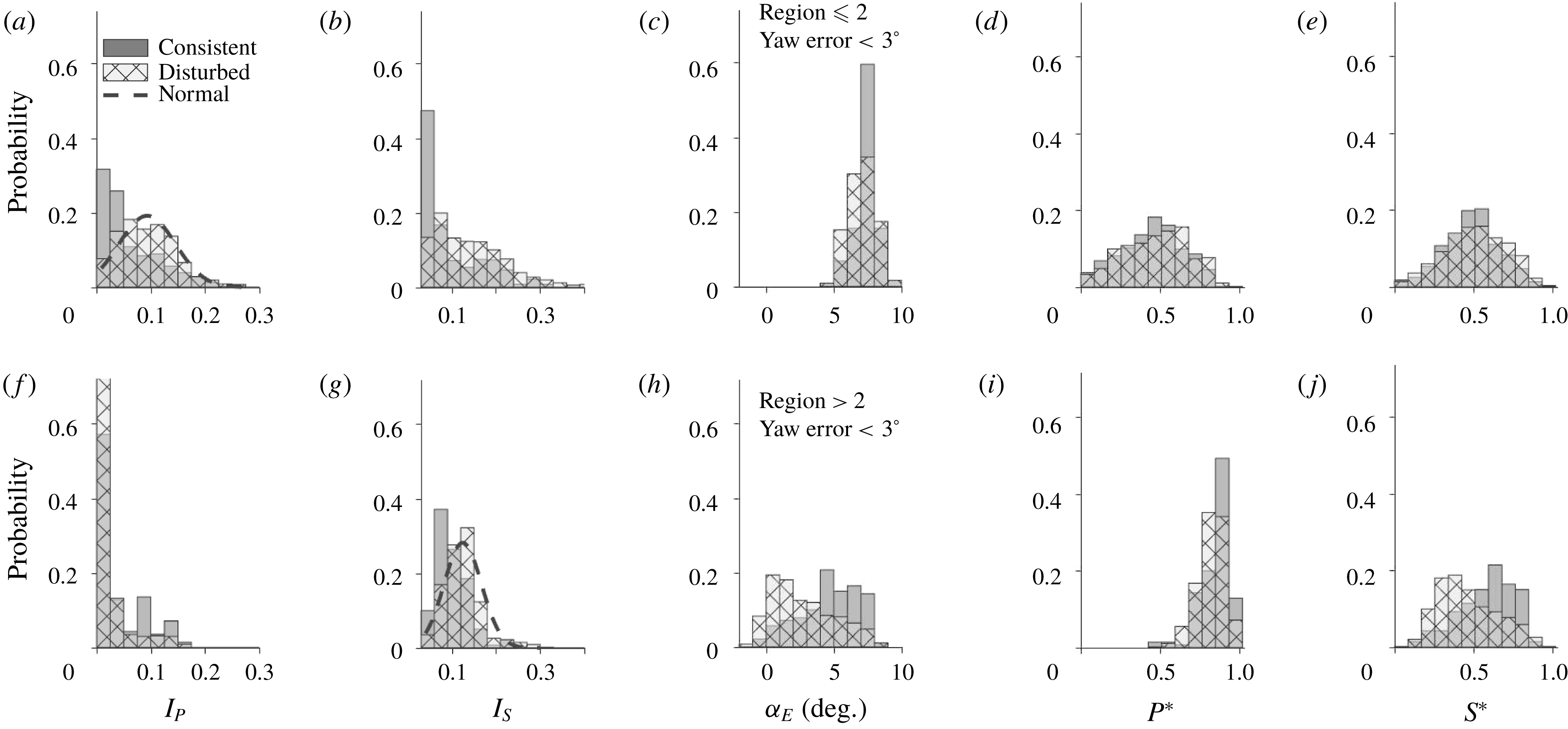
Figure 16(a) shows the power fluctuation
 $I_{P}$
histogram, in which considerable separation is observed between the consistent and disturbed states of the tip vortices when turbine operation is restricted to the regions
 ${\leqslant}2$
. Compared to figure 15(d), the centre of the
 $I_{P}$
histogram of the disturbed state clearly shifts towards higher values of
 $I_{P}$
, and its distribution approximates a normal distribution with a peak value of 0.09 and a standard deviation of 0.05. In regions
 ${\leqslant}2$
, the turbine power is directly proportional to the thrust on the turbine, thus a fluctuation in power is manifested as a fluctuation of the tower strain. As a result, the distribution of tower strain fluctuation
 $I_{S}$
presented in figure 16(b) shows similar trends as those of figure 16(a). Moreover, compared to figure 15(e), the distribution of the disturbed state is less clear with a restriction on regions
 ${\leqslant}2$
, while the
 $I_{S}$
distribution for consistent state becomes more concentrated to the region of very low
 $I_{S}$
. Restricting turbine operation to regions
 ${\leqslant}2$
limits the effective angle of attack
 $\unicode[STIX]{x1D6FC}_{E}$
to high values (i.e. 99 % incidence above
 $5^{\circ }$
), as shown in figure 16(c), where no clear separation is observed between the histograms of the consistent and disturbed states. Figure 16(d,e) shows the histograms of normalized turbine power
 $P^{\ast }$
and tower strain
 $S^{\ast }$
in regions
 ${\leqslant}2$
. Similar to those for all regions, no appreciable separation between the consistent and disturbed state is observed.
When the turbine operates in regions
 ${>}2$
, as shown in figure 16(f–j), all histograms show a noticeable discrepancy compared to those presented in figure 16(a–e). One essential cause for such a discrepancy is the TCU auto-adjustment. When operating in regions
 ${>}2$
, the turbine is able to generate power close to (or even exceeding) the rated power, therefore the TCU curbs the power fluctuation to protect the turbine from excessive thrust loads while still maintaining the designed power output. As a result, figure 16(f) shows that the
 $I_{P}$
distribution in regions
 ${>}2$
is largely concentrated in the lower values of
 $I_{P}$
compared to figure 16(a). Specifically, more than 50 % of the consistent states and more than 75 % of the disturbed states of tip vortices are observed in the range of
 $0<I_{P}<0.025$
. In region
 ${>}$
2, due to the effect of power regulation and blade pitching, the correlation between power and strain fluctuations diminishes, evidenced by the significant difference between
 $I_{P}$
histogram (figure 16
f) and
 $I_{S}$
histogram (figure 16
g) in this region. Moreover, a separation for consistent and disturbed tip vortex states is observed in figure 16(g). The least square fit of the
 $I_{S}$
histogram of the disturbed state yields a normal distribution with a mean value of 0.12 and a standard deviation of 0.04, similar to that shown in figure 15(e) without a turbine region restriction. Regarding the effective angle of attack
 $\unicode[STIX]{x1D6FC}_{E}$
, the restriction of the turbine to higher regions causes the distribution of
 $\unicode[STIX]{x1D6FC}_{E}$
to spread towards lower values as opposed to that of regions
 ${<}2$
. More remarkably, such region restriction leads to clear separation between the consistent and disturbed states, with disturbed tip vortices occurring at smaller values of
 $\unicode[STIX]{x1D6FC}_{E}$
and the consistent state concentrated mainly above
 $\unicode[STIX]{x1D6FC}_{E}>5^{\circ }$
. In line with trends observed for
 $\unicode[STIX]{x1D6FC}_{E}$
, the histogram of the normalized tower strain
 $S^{\ast }$
(figure 16
j) also exhibits a clear separation between consistent and disturbed states with a restriction of turbine regions (i.e. regions
 ${>}2$
), due to the inherent connection among blade angle of attack and forces on the turbine blades and tower structures. As for the normalized turbine power
 $P^{\ast }$
(figure 16
i), the restriction of regions
 ${>}2$
shifts the distribution of
 $P^{\ast }$
to the range of
 $0.5<P^{\ast }<1$
for both consistent and disturbed states. A slight separation between the distributions of the two states is observed in comparison with the corresponding figure of regions
 ${<}2$
(figure 16
d), but is not as appreciable as the trends shown for
 $\unicode[STIX]{x1D6FC}_{E}$
and
 $S^{\ast }$
. To summarize, the conditional sampling based on turbine operational regions yields clearer correlations between tip vortex behaviour and turbine operation/response parameters, manifested as separation of the distributions of
 $I_{P}$
,
 $I_{S}$
;
 $P^{\ast }$
,
 $S^{\ast }$
and
 $\unicode[STIX]{x1D6FC}_{E}$
according to the consistent and disturbed states of the tip vortices. Nevertheless, the trends of such separation of distributions are dependent on specific turbine operational regions. In particular, no separation is observed for
 $P^{\ast },S^{\ast }$
and
 $\unicode[STIX]{x1D6FC}_{E}$
in lower turbine regions (
 ${\leqslant}2$
).
To further elucidate the intricate connection between disturbed tip vortex patterns and turbine operation/response, a conditional sampling of specific types of disturbed state is implemented in addition to the yaw and turbine operational region restrictions. Specifically, we choose to focus on the Type I disturbed state in the analysis here for the following reasons. Firstly, the underlying aerodynamic origin of the Type I disturbed state is strongly connected to turbine performance. For example, the reduction of turbine power generation causes a drastic weakening of tip vortices, which further results in the disappearance of the tip vortex signature in the near wake under highly turbulent atmospheric conditions. Therefore, it is reasonable to expect that the conditional sampling based on the Type I disturbed state would improve the correlation of tip vortex behaviour with turbine power and tower strain which is inherently connected to the power generation. Secondly, the Type I disturbed state corresponds to complete disappearance of the voids, whose flow features can be distinguished from those of Type II and III in a non-ambiguous way. Figure 17 shows the histograms of the effective angle of attack
 $\unicode[STIX]{x1D6FC}_{E}$
, normalized turbine power
 $P^{\ast }$
and normalized tower strain
 $S^{\ast }$
for consistent and Type I disturbed tip vortex states under the yaw and region restrictions. The histograms of
 $I_{P}$
and
 $I_{S}$
do not yield a significant difference compared to those in figure 16, and therefore, are not presented here for brevity. As the figure shows, in the lower turbine regions (
 ${\leqslant}2$
), the distribution of the Type I disturbed state (figure 17
a) is slightly shifted to the region of low
 $\unicode[STIX]{x1D6FC}_{E}$
in comparison to that of all disturbed states shown in figure 16(c). A similar trend is also observed for
 $P^{\ast }$
(figure 17
b). Note that the conditional sampling at this stage (i.e. yaw error, turbine region and disturbed state type) substantially reduces the number of samples available for statistical analysis, which makes some histograms appear choppy. This issue limits the further analysis of the data based on conditional sampling, and we expect to resolve this issue through more data recording in future deployments. In higher turbine regions (
 ${>}2$
), as shown in figure 17(d–f), the histograms generally resemble those shown in figure 16(h–j), indicating that the majority of disturbed tip vortices in higher turbine regions are in the Type I state. Nevertheless, with a restriction on the type of disturbed state, there is a measurable increase of separation between the distributions for the disturbed and consistent states in the
 $\unicode[STIX]{x1D6FC}_{E}$
,
 $P^{\ast }$
and
 $S^{\ast }$
histograms. Such a separation increase is manifested by 10 %–15 % of the samples of the disturbed state shifting towards lower values and the distribution of the consistent state staying relatively unchanged in comparison to the corresponding ones in figure 16.
The probability histograms of effective angle of attack (
 $\unicode[STIX]{x1D6FC}_{E}$
), turbine power (
 $P^{\ast }$
) and tower strain (
 $S^{\ast }$
) for consistent and Type I disturbed tip vortex states under a restriction of yaw error
 ${<}3^{\circ }$
for (a–c) turbine operational regions
 ${\leqslant}2$
and (d–f) turbine operational regions
 ${>}2$
.
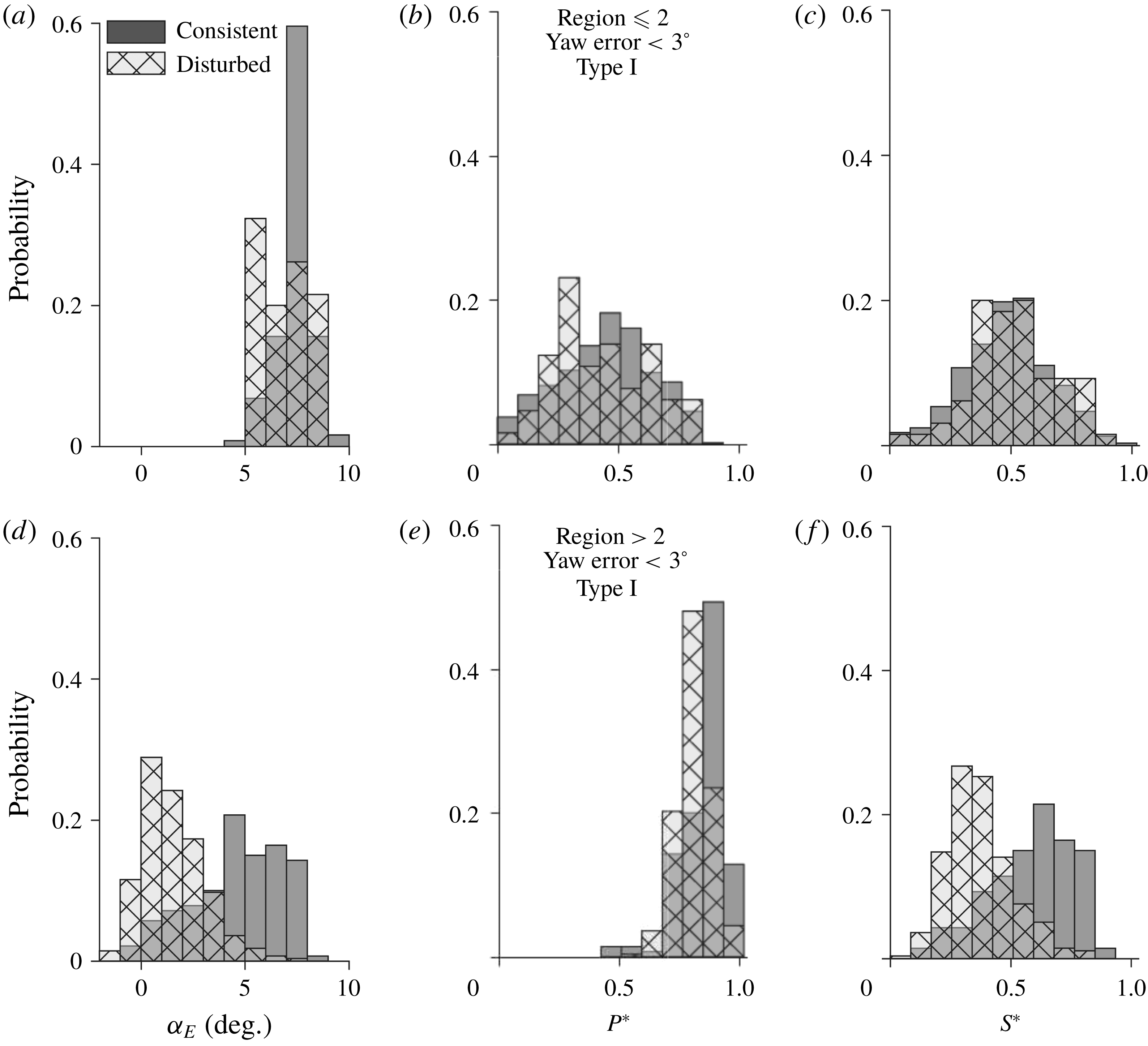
In addition to the histograms of turbine operational/response parameters, the direct correspondence between the tip vortex behaviour and turbine operation/response is examined by marking the incidences of disturbed states of tip vortices in the time series of these parameters. Note that, under field conditions, the characteristics of tip vortices are inevitably influenced by multiple physical variables, and therefore, it is difficult to establish a one-to-one correspondence between tip vortex behaviour and a specific turbine operational/response parameter unless stringent conditional sampling is imposed. Figure 18 presents two sample time series of turbine operation/response parameters marked with regions corresponding to the occurrence of the disturbed turbine states. The first sample displays the variation of
 $\unicode[STIX]{x1D6FC}_{E}$
in a period of approximately 350 s with the incidences of all types of disturbed states marked by the grey vertical bands (figure 18
a). The specific time sequence is chosen such that the turbine operation is confined to regions
 ${\leqslant}2$
(approximately 96 % of the time here), yaw error is restricted to
 ${<}3^{\circ }$
and the average value of
 $I_{P}$
for the time period is around 0.1. These restrictions allow us to sample the data only in the region around the probability peak of the disturbed state, as shown in figure 16(a). As shown in figure 18(a), the grey vertical bands occur almost exclusively in the time periods around local minima of
 $\unicode[STIX]{x1D6FC}_{E}$
, indicating the consistent generation of tip vortices is likely to be disturbed when the utility-scale turbine operates under low
 $\unicode[STIX]{x1D6FC}_{E}$
and experiences sharp changes of
 $\unicode[STIX]{x1D6FC}_{E}$
. The second sample shows the change of
 $S^{\ast }$
in a period of 1790 s with incidences of the Type I disturbed state marked by the grey vertical bands (figure 18
b). This sample time series, corresponding to a time period with the lowest wind speed fluctuations among all of the datasets, is selected to allow clear demonstration of the one-to-one correspondence between tip vortex behaviour and turbine operations. In addition, similar to that in figure 18(a), a yaw error restriction (
 ${<}5^{\circ }$
) is imposed on the data to minimize the effect of yaw misalignment on the results. Note that the yaw error restriction is relaxed and no turbine region restriction is imposed here in comparison to previous cases to retain as many Type I disturbances as possible. Figure 18(b) illustrates that most Type I disturbed states tend to occur in the vicinity of the local minima associated with a sudden large drop of
 $S^{\ast }$
. Such a drop in
 $S^{\ast }$
is strongly correlated with a significant loss of the lift generated by the turbine blades, resulting in drastic weakening of the tip vortices (i.e. a major cause of the Type I disturbed state of tip vortices). The general trend observed here is consistent with the histograms shown in figure 17(f). In addition, the time series suggests that Type I disturbances have a higher tendency to occur in the periods when the turbine operations or the incoming wind fluctuations cause a significant lowering of turbine loading.
Samples of time series of (a) effective angle of attack (
 $\unicode[STIX]{x1D6FC}_{E}$
) with incidences of disturbed states marked using grey vertical bands and (b) normalized tower strain (
 $S^{\ast }$
) with incidences of the Type I disturbed state marked using grey vertical bands.

4 Conclusions and discussion
4.1 Conclusions
Using super-large-scale particle image velocimetry (SLPIV) and flow visualization with natural snow, this study presents the first systematic experimental investigation of the velocity field and the coherent vortex structures in the near wake of a utility-scale wind turbine at unprecedented spatial and temporal resolution. The turbulent flow field for a time duration of 30 min is first examined using the SLPIV measurements in the deployment on 3 February, 2016, which has a field of view (FOV) of 115 m (vertical)
 $\times$
66 m (streamwise) centred 0.41
 $D$
downstream of the turbine tower and 0.19
 $D$
offset from the central tower plane. The time-averaged wake velocity field exhibits a clear non-Gaussian distribution with a slight upsurge of streamwise velocity at elevations around the turbine hub height. Combined with the incoming velocity profile estimated from the wind measurements using a met tower near the turbine, the time-averaged profile of the wake deficit is obtained and compared with those from a wind tunnel experiment and a field measurement using lidar at similar locations in the near wake of a turbine. The comparison shows significant differences across these profiles around the same downstream location of the turbine (
 $x=0.41D$
), potentially due to the spanwise offset of the measurement planes and the difference in turbine conditions across these studies. Nevertheless, the wake deficit averaged over the turbine blade span is calculated to be 0.29 from SLPIV, within close proximity of the values obtained from the wake models proposed in a number of prior studies. The in-plane turbulent kinetic energy (TKE), i.e.
 $k_{xz}$
, shows a region of relatively low
 $k_{xz}$
around the hub height with local maxima of
 $k_{xz}$
in the region between the hub height and the elevation corresponding to the turbine blade tips.
The instantaneous velocity fields from SLPIV indicate the presence of intermittent wake contraction states which are in clear contrast with the expansion states typically associated with wind turbine wakes. These contraction states feature a pronounced upsurge of velocity in the central portion of the wake. The wake velocity ratio
 $R_{w}$
, defined as the ratio of the spatially averaged velocity of the inner wake to that of the outer wake, is introduced to categorize the instantaneous near wake into expansion (
 $R_{w}<1$
) and contraction states (
 $R_{w}>1$
). Based on the
 $R_{w}$
criterion, the wake contraction occurs 25 % of the time during the 30 min time duration of the SLPIV measurements, consistent with the numerical simulation of Sebastian & Lackner (Reference Sebastian and Lackner2011). Based on the available literature, we attribute wake transitions to the sudden drop in the effective angle of attack (
 $\unicode[STIX]{x1D6FC}_{E}$
) and the rate of change of blade pitch (
 $\text{d}\unicode[STIX]{x1D6FD}/\text{d}t$
). It is found that the histograms of the expansion and contraction states show a significant separation over
 $\text{d}\unicode[STIX]{x1D6FD}/\text{d}t$
while such separation over
 $\unicode[STIX]{x1D6FC}_{E}$
is less clear. The samples of time sequences of
 $\text{d}\unicode[STIX]{x1D6FD}/\text{d}t$
and
 $R_{w}$
further substantiate the strong connection between the wake state transition and the rate of change of blade pitch. Moreover, blade pitch change is found to be strongly correlated to the tower and blade strains measured on the turbine, establishing the crucial physical link for the occurrence of wake contractions. This result suggests that the flexing of the turbine tower and the blades could indeed lead to the interaction of the rotor with the turbine wake, and cause wake contraction, as indicated by prior studies.
Based on the datasets obtained from multiple deployments conducted in 2014–2016, the tip vortices, visualized as snow voids, are analysed and correlated with turbine operation/response parameters including normalized turbine power (
 $P^{\ast }$
), normalized turbine tower base strain (
 $S^{\ast }$
), the fluctuation intensity of power (
 $I_{P}$
) and that of tower strain (
 $I_{S}$
) as well as the effective angle of attack (
 $\unicode[STIX]{x1D6FC}_{E}$
). The tip vortex behaviour is categorized into a consistent state and various disturbed states (Types I, II and III) according to different snow void patterns. The histograms corresponding to the consistent and disturbed states are examined over the aforementioned turbine operation/response parameters with different conditional sampling restrictions. With yaw error restriction, it is revealed that the histogram of consistent states follows a clear exponential distribution spanning a region of very low
 $I_{S}$
, while the disturbed state exhibits a normal distribution with a mean value of
 $I_{S}$
significantly higher than that of the consistent state. Imposing further restriction on turbine operational regions, the
 $I_{P}$
histograms also show trends similar to the
 $I_{S}$
histograms but only for lower regions (i.e. regions
 ${\leqslant}2$
) of operation owing to the strong correlation between power and tower strain in lower regions. For higher regions (
 ${>}2$
), the
 $\unicode[STIX]{x1D6FC}_{E}$
,
 $P^{\ast }$
and
 $S^{\ast }$
histograms display clear separation for the consistent and disturbed states with disturbed states occurring towards lower values for all of the respective histograms. Further restricting the analysis to the Type I disturbed state makes the above trends clearer owing to the inherent aerodynamic connection with the turbine performance characteristics. In the end, samples of time series of
 $\unicode[STIX]{x1D6FC}_{E}$
and
 $S^{\ast }$
are selected to demonstrate the direct correspondence between tip vortex behaviours and turbine operation/responses, which shows that most disturbance events occur in the vicinity of the local minima associated with sudden large drops in
 $\unicode[STIX]{x1D6FC}_{E}$
and
 $S^{\ast }$
.
4.2 Discussion
The velocity field measurements within the near wake of the utility-scale turbine could serve as benchmark datasets for wind turbine wake research (i.e. laboratory, field and computational studies). The velocity deficits measured using SLPIV can be employed to validate and potentially improve the existing wake models derived from prior studies. The measurements will benefit laboratory-scale studies by providing a direct reference for controlled experimentation and improve the design of experiments to address the scalability issues. As current field-scale techniques (e.g. lidar and sodar) are typically deployed to capture large-scale wake patterns (primarily the far wake) considering their coarse spatial and temporal resolution, our measurements in the near wake could provide a crucial link of turbulence–turbine interaction and whole wake characteristics. The numerical studies on wind turbine wakes could also utilize the velocity deficit and TKE measurements to improve the high-fidelity simulation techniques that can predict the most realistic wake characteristics and evolution. We acknowledge our measurements are limited to the region adjacent to the turbine and to a specific spanwise location (0.19
 $D$
) with very few prior studies available for direct comparison. However, the datasets are still invaluable considering the dearth of reliable data at utility scale. For example, a study similar to the current work but in a different spanwise location would provide further useful information which could all be combined together to arrive at the complete three-dimensional structure of the turbulent near wake. Such further studies will also explain the discrepancies in the velocity deficit and TKE measurements noticed in the current work. In general, longer time sequences collected in line with the current work at multiple spanwise locations under different turbine operational conditions are needed for a robust comparison with the available literature.
The paper presents the first field evidence and the quantification of the intermittent wake transition occurring in the near wake of a utility-scale turbine, which has been only discussed minimally in prior analytical and numerical simulation studies. Such intermittent near-wake transition from the expansion to contraction state can have a profound effect on the wake evolution (e.g. near-wake length, wake recovery) downstream. It could significantly alter the entire wake structure, including the vortex interaction, turbulence characteristics (e.g. mixing and momentum exchange across the wake shear layer) and overall wake instability. Although an extensive literature has shown the influence of atmospheric turbulence on wake recovery, the effect of these wake state transitions caused by turbulence–turbine interaction presented in the current study has not been identified. Our results have shown that the wake contraction state occurs for a substantial portion (i.e. approximately 25 % of the time) of regular operation time of a utility-scale wind turbine, necessitating the incorporation of such a phenomenon into the physics-based wake models for future wind farm designs. In addition, through both statistical analysis and instantaneous correspondence, our study has made the first attempt to establish a connection between the transitions of wake states and the parameters that can be derived from turbine SCADA data. Such information can be potentially used to develop advanced turbine control algorithms for existing and next-generation ‘smart’ wind farms. However, we acknowledge that our current analysis of wake transition relies on the specification of the
 $R_{w}$
criterion and appropriate filtering of the turbine operation/response parameters, which involves a number of uncertainties. For example, the
 $R_{w}$
criterion can be affected by the choice of inner/outer wake domains, the limited characterization of the entire wake based on the data from one spanwise location, the uncertainties from the smoothing and time corrections of the aerodynamic parameters and atmospheric turbulence, etc. Additionally, despite some support from the literature, the precise mechanism governing the reported wake transition is still speculative in the current analysis. To address these issues, further investigation will focus on acquiring more near-wake SLPIV data at multiple spanwise locations and under different turbine operational conditions to gain a better statistical understanding of these wake transitions as the current analysis is based on only 30 min of data. Moreover, there is a need to integrate our experimental work with state-of-the-art numerical studies to fully elucidate the underlying mechanism of these intermittent wake transitions, and potentially incorporate such unsteady effects into simulations to arrive at a more realistic and reliable prediction of wake behaviours. Nevertheless, our analysis suggests the flexing of the turbine tower structure and the blades in the fore–aft direction, owing to the typical size and mechanical properties of utility-scale turbines, could contribute to wake transitions. This result highlights the significance of understanding flow–structure interaction involved in utility-scale wind turbine operation, and the potential for increasing the efficiency of wind turbines through improvement of their structural robustness and operational strategies.
The tip vortex analysis presented in our paper reveals interesting correlations between the tip vortex patterns and the turbine operation/response parameters. Similar to the wake transition results mentioned above, such information can be potentially employed for developing novel turbine control strategies for wind farm optimization. Specifically, on the one hand, tip vortex behaviour is an effective indicator of overall wake stability (Ivanell et al. Reference Ivanell, Mikkelsen, Sørensen and Henningson2010), the information of which can be used in physics-based wake models for more accurate prediction of wake evolution. On the other hand, the turbine operation/response parameters used for correlating with the tip vortex behaviours are/can be derived from readily available turbine SCADA inputs, facilitating the direct incorporation of such information into individual turbine or wind farm controls. Although the current study incorporated deployments from multiple years, the trends exhibited in the histograms highlight the need for more data to achieve converged statistical distributions under stringent conditional sampling. The subtle differences between the different types of tip vortex disturbances and their underlying causes could not be studied in detail for the same reason. Hence all the near-future deployments will aim at collecting tip vortex behavioural data along with whole wake measurements.
In summary, the current study provides a detailed analysis of the near-wake flow field of a utility-scale wind turbine, including interesting intermittent wake transitions and tip vortex patterns, and establishes a statistics-based linkage between these wake behaviours and turbine operational/response parameters. This study not only offers benchmark datasets for comparison with the-state-of-the-art numerical simulation, laboratory and field measurements, but also sheds light on understanding wake characteristics and their downstream development, turbine performance and regulation, as well as developing novel turbine or wind farm control strategies. Following the methodology presented in the current paper, the future study will focus on investigating the three-dimensional structure of the near wake with data from multiple spanwise locations and establishing a more detailed and robust statistical description of the wake behaviours with extended datasets under each specific turbine operational condition.
Acknowledgements
This work was supported by the National Science Foundation CAREER award (NSF-CBET-1454259), Xcel Energy through the Renewable Development Fund (grant RD4-13) as well as IonE of University of Minnesota. We also thank the faculties and engineers from St Anthony Falls Laboratory, including M. Guala, K. Howard, S. Riley, J. Tucker, J. Mullin, C. Ellis, J. Marr, C. Milliren and D. Christopher, for their assistance in the experiments.
Supplementary movies
Supplementary movies are available at https://doi.org/10.1017/jfm.2018.779.