

1 Introduction
Interactions between opposing waves and currents have long been known as potentially hazardous to shipping. In 2015 the Cemfjord cement carrier was found capsized in the Pentland Firth of Scotland; the concluding report stated that ‘Cemfjord capsized suddenly and rapidly at 13.16 on 2 January 2015 when it encountered extraordinarily violent, breaking seas  $(\cdots \,)$ created by gale force winds opposing a strong ebb tidal stream’ (Marine Accident Investigation Branch 2016). While these effects of opposing waves and currents on shipping have been understood qualitatively by seafarers for centuries, only in the latter half of the 20th century, did these interactions become the subject of research (as reviewed in the seminal papers by Peregrine (Reference Peregrine1976) and Peregrine & Jonsson (Reference Peregrine and Jonsson1983)). Waves meeting an opposing current are known to increase in amplitude,
 $a$, and wavenumber,
 $k$, a combination which causes an overall increase in steepness,
 $\unicode[STIX]{x1D716}\propto ka$. The relationship between wavenumber and frequency (dispersion relation) is fundamental to the evolution of dispersive waves through all media, and thus wave–current interactions are important, as they affect the dispersion relationship. Additionally, the increase in steepness not only makes waves more prone to violent breaking but can also bring otherwise linear waves into a parameter space subject to amplitude-dependent nonlinear effects such as modulational instability.
Modulational instability affects medium- and high-steepness, narrow-banded waves propagating on water deeper than  $k_{0}d=1.36$ (with
 $k_{0}$ being the carrier wavenumber and
 $d$ the water depth). At first order, wavetrains subject to modulational instability experience exponential amplitude growth of their sideband components, seen as a pulsing or modulation in the time domain with extreme wave crests often being formed (Benjamin & Feir Reference Benjamin and Feir1967; Hasimoto & Ono Reference Hasimoto and Ono1972). The nonlinear Schrödinger equation (NLSE) provides the simplest framework for investigating this phenomenon and admits a number of solutions exhibiting modulational instability. One such family of analytic solutions is the ‘breather wave’ family named for the manner in which their envelope amplitudes (periodically) increase to 3 or 5 times that of their initial amplitude (Ma Reference Ma1979; Chabchoub, Hoffmann & Akhmediev Reference Chabchoub, Hoffmann and Akhmediev2011; Chabchoub et al. Reference Chabchoub, Hoffmann, Onorato and Akhmediev2012). Whereas breather waves require precise initial conditions to complete their prescribed evolution, unstable Stokes plane waves provide a more general context for investigating modulational instability. Stokes plane waves exhibit modulational instability when sideband frequency perturbations are introduced to a carrier wave within a range of unstable perturbation wavenumbers (found through linear stability analysis) (Yuen & Lake Reference Yuen and Lake1982). Many experiments have been carried out on the breakdown of unstable wavetrains following the pioneering studies by Benjamin & Feir (Reference Benjamin and Feir1967), Yuen & Lake (Reference Yuen and Lake1982), Melville (Reference Melville1982); and Lake et al. (Reference Lake, Yuen, Rungaldier and Ferguson1977).
In their simplest form, sub-surface currents exist as one-dimensional and uniform with depth. Waves initially propagating on still water that begin to interact with such a uniform current, experience alterations in amplitude and wavelength in accordance with the conservation of wave action, first derived for low-steepness linear waves by Bretherton & Garrett (Reference Bretherton and Garrett1968) and Whitham (Reference Whitham1965) then subsequently extended to nonlinear waves by Andrews & McIntyre (Reference Andrews and McIntyre1978). In essence, opposing currents tend to increase amplitude and shorten wavelength, whereas for following currents the reverse is true, as captured by the uniform-current linear dispersion relationship and the conservation of wave action. In real flows that often experience bed friction and surface winds, variations in inline current velocity with depth introduce vertical shear to the flow.
The most complex forms of sheared current exist as arbitrary variations in all 3-component velocities,  $(U,V,W)$ within a fluid. Nonlinear numerical models for two-dimensional waves and arbitrary distributions of vorticity by Dalrymple (Reference Dalrymple1977) and Thomas (Reference Thomas1990) have been shown to agree very well with laboratory experiments (Swan, Cummins & James Reference Swan, Cummins and James2001). However, their complexity generates a need for analytic approximations to the dispersion relationship. These have been derived for moderate shear (Skop Reference Skop1987; Kirby & Chen Reference Kirby and Chen1989), weak shear (Swan & James Reference Swan and James2000) and high depth-averaged shear rates (Ellingsen & Li Reference Ellingsen and Li2017). In addition to direct changes to the free surface, shear affects sea bed pressure measurements and the transfer functions used to determine free surface elevation from bottom pressure (Constantin & Strauss Reference Constantin and Strauss2004). While the effect of arbitrary vorticity on determining surface elevation from pressure measurements is known (Henry Reference Henry2013), only recently have the pressure transfer functions and amplification factors been derived for the most general case (Henry & Thomas Reference Henry and Thomas2017). Often, investigations into the effects of sheared current on wave behaviour constrain current velocity variation to one dimension.
Horizontally sheared currents can take the form of inline velocities that vary either along the axis of wave propagation or perpendicular to it. Propagation of waves across an inline horizontally sheared current ( $\text{d}U/\text{d}x\neq 0$) and onto an opposing current has the effect of steepening waves by the conservation of wave action. Experiments have shown this process to trigger rogue waves in random unidirectional Gaussian wave spectra (Toffoli et al. Reference Toffoli, Waseda, Houtani, Cavaleri, Greaves and Onorato2015) as well as to destabilise regular wavetrains (Onorato, Proment & Toffoli Reference Onorato, Proment and Toffoli2011). Jet-type horizontally sheared currents (
 $\text{d}U/\text{d}y\neq 0$) are known to exist in the Agulhas current around the South African east coast (Mallory Reference Mallory1974). These jet currents are of interest as a possible mechanism of rogue wave formation through wave trapping (Shrira & Slunyaev Reference Shrira and Slunyaev2014).
Assuming a steady, one-dimensional, linearly varying current velocity with depth (constant vorticity) allows the addition of irrotational perturbations (in the form of waves) and therefore the assumption of a potential fluid and the simplified governing equations this implies (Ellingsen & Brevik Reference Ellingsen and Brevik2014). For a rotational flow of constant vorticity, the dispersion equation for linear waves was first derived independently by both Thompson (Reference Thompson1949) and Biésel (Reference Biésel1950). The evolution of steep waves on constant shear has been investigated numerically (using the Euler equations) (Dalrymple Reference Dalrymple1974; Da Silva & Peregrine Reference Da Silva and Peregrine1988; Vanden-Broeck Reference Vanden-Broeck1996), and its effect on modulational instability found to be destabilised by positive shear and vice versa (Choi Reference Choi2009). It should be noted that linear waves initially on still water approaching an opposing constant vorticity current are steepened in a similar manner to the uniform-current case, by wave action conservation altered for constant vorticity (Quinn, Toledo & Shrira Reference Quinn, Toledo and Shrira2017).
The same effects of constant vorticity on wave stability found through numerical analysis, have also been found through constant vorticity NLSEs (so-called vor-NLSEs) as derived analytically for infinite depth and studied numerically for arbitrary depth by Baumstein (Reference Baumstein1998). Thomas, Kharif & Manna (Reference Thomas, Kharif and Manna2012) (henceforth TKM12) derived a constant vorticity NLSE with coefficients expressed as explicit functions of the carrier wave properties, vorticity and depth, which is the starting point of the present paper. Linear stability analysis of the vor-NLSE has also shown that when the ratio of shear,  $\unicode[STIX]{x1D6FA}$, to carrier wave frequency,
 $\tilde{\unicode[STIX]{x1D714}}_{0}$ (in the surface current reference frame, denoted with tilde) is less than
 $-2/3~\text{rad}^{-1}$ (i.e.
 $\unicode[STIX]{x1D6FA}/\tilde{\unicode[STIX]{x1D714}}_{0}<-2/3~\text{rad}^{-1}$) wavetrains become entirely stabilised regardless of perturbation wavenumber or depth.
Further to the aforementioned Doppler shift of waves propagating on a current, a two-way exchange of energy and momentum between waves and currents may create a velocity field more complex than the simple superposition of individual periodic and mean flow solutions (see Jonsson, Brink-Kjaer & Thomas (Reference Jonsson, Brink-Kjaer and Thomas1978) and Craik (Reference Craik1988) for the literature discussing such interaction). Coupled nonlinear interaction equations for plane waves on uniform currents have been derived by Baddour & Song (Reference Baddour and Song1990a,Reference Baddour and Songb) and predict reductions in current velocity during adverse wave–current interaction and vice versa. The change in shear rate of constant vorticity currents and colinear waves has been measured in experiments by Klopman (Reference Klopman1994) using laser Doppler velocimetry. Groeneweg & Klopman (Reference Groeneweg and Klopman1998) compare these experiments to numerical solutions of the equation they derive based on the generalised Lagrangian mean, finding good agreement and showing an increase in vertical shear near the surface in adverse currents and vice versa. In this study, we do not consider the effect of the waves on the current’s magnitude and shear rate and acknowledge that full velocity field measurements in the presence of waves could improve the robustness of our conclusions.
This paper investigates experimentally the propagation of medium-steepness weakly nonlinear waves on a current profile that is steady, one-dimensional, has constant vorticity and opposes the wave direction. The steepening behaviour that takes place as the waves come into contact with the current is not examined. Instead, the focus is placed on the evolution of the waves once they are on the current. In doing so, the effect of a vertical shear is investigated and not the magnitude of the current itself. In particular, the effects of vertical shear on the (linear) dispersion relationship and on the occurrence of modulational instability are investigated experimentally in parts I and II of this paper respectively. It is found that in all experiments, the constant vorticity equations predicted wave linear evolution and stability very well, out-performing the zero vorticity equations.
This paper is laid out as follows. Section 2 reviews the derivation of the constant vorticity nonlinear Schrödinger equation (vor-NLSE) and the constant vorticity dispersion (vor-dispersion) relationship. Section 3 discusses the method used to create a linearly sheared current profile, collect wavelength and frequency measurements from low-steepness regular waves and measure the stability of weakly nonlinear modulated waves. Section 4 discusses the linear and weakly nonlinear wave evolution measurements and how both compare to predictions by constant vorticity and zero vorticity equations. Finally, conclusions are drawn in § 5.
2 Theoretical model
2.1 Coordinate system and reference frames
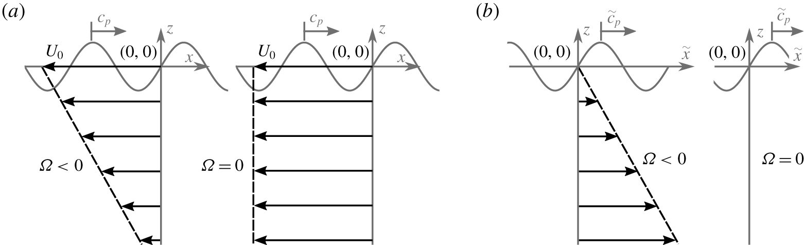
Figure 1 presents the coordinate system used in both the laboratory and the surface current reference frames. The system is assumed two-dimensional, such that it is invariant along the transverse  $y$-axis. The location of the still water level is at
 $z=0$, the free surface elevation at
 $z=\unicode[STIX]{x1D702}(x,t)$, and the bed at
 $z=-d$. The constant vorticity wave equations (vor-equations) are typically derived in the surface current reference frame. In the laboratory reference frame, the steady, inline current profile,
 $U(z)$ with constant shear,
 $\unicode[STIX]{x1D6FA}=\text{d}U/\text{d}z$, is prescribed in the
 $x$-direction. This constant surface current velocity,
 $U_{0}$ and shear rate,
 $\unicode[STIX]{x1D6FA}$ define the current field as,
 $$\begin{eqnarray}U=U_{0}+\unicode[STIX]{x1D6FA}z.\end{eqnarray}$$
All experiments presented herein consider waves propagating in the positive  $x$-direction, while current profiles are opposing, and associated velocities are therefore negative. Wave frequencies measured in the laboratory reference frame,
 $\unicode[STIX]{x1D714}$ can be related to wave frequencies in the surface current reference frame,
 $\tilde{\unicode[STIX]{x1D714}}$ using a simple Doppler shift,
 $$\begin{eqnarray}\unicode[STIX]{x1D714}=\tilde{\unicode[STIX]{x1D714}}+U_{0}k,\end{eqnarray}$$
where  $k$ is wavenumber, and the tilde denotes properties measured in the surface current reference frame.
Schematic of laboratory (a) and surface current (b) reference frames used herein. Both reference frames show a negatively sheared current on the left ( $U_{0}<0$,
 $\unicode[STIX]{x1D6FA}<0$) and negative uniform current on the right (
 $U_{0}<0$,
 $\unicode[STIX]{x1D6FA}=0$) with respect to the
 $x$-direction, the direction of the wave phase velocity,
 $c_{p}$. The tilde denotes properties measured within the surface current reference frame.

2.2 Governing equations and boundary conditions
In general, potential flow theory cannot be used in the presence of vorticity. The one exception is a strictly two-dimensional flow with waves travelling either exactly opposing or inline with the current and with the current’s vorticity being constant in time and space, as considered here. The total velocity field  $\boldsymbol{u}$ can be written as the sum of a rotational current and irrotational water waves:
 $\boldsymbol{u}=U(z)\hat{\boldsymbol{i}}+\unicode[STIX]{x1D735}\unicode[STIX]{x1D719}$, where
 $\hat{\boldsymbol{i}}$ is the unit vector in the
 $x$-direction and
 $\unicode[STIX]{x1D719}$ is the potential of the waves. The potential,
 $\unicode[STIX]{x1D719}$ of the system must satisfy the Laplace equation,
 $\unicode[STIX]{x1D6FB}^{2}\unicode[STIX]{x1D719}=0$ in the range
 $-d<z<\unicode[STIX]{x1D702}(x,t)$ and is related to the streamfunction of the waves,
 $\unicode[STIX]{x1D713}$ through the Cauchy–Riemann equations. Kelvin’s circulation theorem shows that an irrotational streamfunction can be assumed when vorticity within the flow is constant in space and time (Da Silva & Peregrine Reference Da Silva and Peregrine1988). The standard bottom boundary condition,
 $\unicode[STIX]{x1D719}_{z}=0$ at
 $z=-d$ prevents flow through the bed. At the surface, the kinematic and dynamic boundary conditions are respectively,
 $$\begin{eqnarray}\displaystyle & & \displaystyle \unicode[STIX]{x1D702}_{t}+(\unicode[STIX]{x1D6F7}_{x}+\unicode[STIX]{x1D6FA}\unicode[STIX]{x1D702})\unicode[STIX]{x1D702}_{x}-\unicode[STIX]{x1D6F7}_{z}=0\quad \text{and}\quad \unicode[STIX]{x1D6F7}_{t}+{\textstyle \frac{1}{2}}\unicode[STIX]{x1D6F7}_{x}^{2}+{\textstyle \frac{1}{2}}\unicode[STIX]{x1D6F7}_{z}^{2}+\unicode[STIX]{x1D6FA}\unicode[STIX]{x1D702}\unicode[STIX]{x1D6F7}_{x}+g\unicode[STIX]{x1D702}-\unicode[STIX]{x1D6FA}\unicode[STIX]{x1D6F9}=0\nonumber\\ \displaystyle & & \displaystyle \quad \text{for }z=\unicode[STIX]{x1D702}(x,t),\end{eqnarray}$$
where  $\unicode[STIX]{x1D6F9}\equiv \unicode[STIX]{x1D713}(z=\unicode[STIX]{x1D702}(x,t))$ and
 $\unicode[STIX]{x1D6F7}\equiv \unicode[STIX]{x1D719}(z=\unicode[STIX]{x1D702}(x,t))$ denote their respective lower case variables evaluated at the free surface, and
 $g$ is the gravitational constant.
2.3 Solutions using perturbation methods
2.3.1 Linear solutions: frequency dispersion
Assuming a carrier wave with amplitude  $a_{0}$, wavenumber
 $k_{0}$ and frequency
 $\tilde{\unicode[STIX]{x1D714}}_{0}$, a Stokes expansion in steepness,
 $\unicode[STIX]{x1D716}=a_{0}k_{0}$ gives at first order the linear, constant vorticity, arbitrary-depth vor-dispersion relation (first derived by Biésel (Reference Biésel1950) and Thompson (Reference Thompson1949)),
 $$\begin{eqnarray}\tilde{\unicode[STIX]{x1D714}}_{0}^{2}+(\tilde{\unicode[STIX]{x1D714}}_{0}\unicode[STIX]{x1D6FA}-gk_{0})\tanh k_{0}d=0.\end{eqnarray}$$
By relating wave frequency to wavenumber, the implicit vor-dispersion relation describes the evolution of linear waves ( $\unicode[STIX]{x1D716}\ll 1$), where nonlinear changes to the dispersion relationship and instability do not play a role. Throughout the present work, frequencies and wavenumbers are computed from (2.2) and (2.4).
2.3.2 The vor-NLSE
Performing a combined Stokes and multiple-scales expansion, Baumstein (Reference Baumstein1998) (for deep water) and subsequently TKM12 (for arbitrary depth) derived a NLSE with coefficients reflecting the presence of vorticity: the vor-NLSE. In their derivations, a carrier wave varying on the fast scales  $x$, and
 $t$ is modulated by a wavepacket evolving on the slow spatial and temporal scales,
 $$\begin{eqnarray}\unicode[STIX]{x1D709}=\unicode[STIX]{x1D716}(\tilde{x}-\tilde{c}_{g}t)\quad \text{and}\quad \unicode[STIX]{x1D70F}=\unicode[STIX]{x1D716}^{2}t,\end{eqnarray}$$
where the group velocity,  $\tilde{c}_{g}$, and the slow scales are defined in the reference frame of the surface current, as denoted by the tilde. At third order in the small parameter
 $\unicode[STIX]{x1D716}$, the nonlinear evolution of a narrow-banded wavepacket of amplitude,
 $A$ is described by the constant vorticity NLSE (vor-NLSE) with linear coefficient,
 $L$, and nonlinear coefficient,
 $M$, (TKM12),
 $$\begin{eqnarray}iA_{\unicode[STIX]{x1D70F}}+LA_{\unicode[STIX]{x1D709}\unicode[STIX]{x1D709}}-M|A|^{2}A=0.\end{eqnarray}$$
For brevity, we present these coefficients for deep water,
 $$\begin{eqnarray}L=-\frac{\tilde{\unicode[STIX]{x1D714}}_{0}(1+\bar{\unicode[STIX]{x1D6FA}})^{2}}{k_{0}^{2}(2+\bar{\unicode[STIX]{x1D6FA}})^{3}}\quad \text{and}\quad M=\frac{\tilde{\unicode[STIX]{x1D714}}_{0}k_{0}^{2}}{8(1+\bar{\unicode[STIX]{x1D6FA}})}(4+10\bar{\unicode[STIX]{x1D6FA}}+8\bar{\unicode[STIX]{x1D6FA}}^{2}+3\bar{\unicode[STIX]{x1D6FA}}^{3}),\end{eqnarray}$$
where  $\bar{\unicode[STIX]{x1D6FA}}=\unicode[STIX]{x1D6FA}/\tilde{\unicode[STIX]{x1D714}}_{0}$. The arbitrary-depth coefficients (used for all calculations herein) can be found in TKM12 (their (48)–(58)) and appendix A of this paper. The first-order free surface is reconstructed using,
 $$\begin{eqnarray}\unicode[STIX]{x1D702}^{(1)}=\text{Re}[\unicode[STIX]{x1D716}A(\unicode[STIX]{x1D709},\unicode[STIX]{x1D70F})\text{e}^{\text{i}(k_{0}\tilde{x}-\tilde{\unicode[STIX]{x1D714}}_{0}t)}].\end{eqnarray}$$
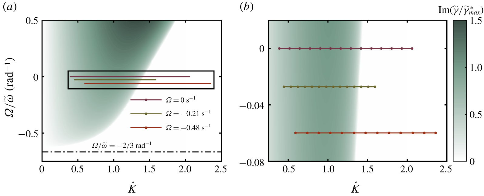
Sideband growth rate,  $\tilde{\unicode[STIX]{x1D6FE}}$ normalised by the maximum growth rate at zero shear,
 $\tilde{\unicode[STIX]{x1D6FE}}_{max}^{\ast }=M^{\ast }a_{0}^{2}$, as a function of normalised perturbation wavenumber,
 $\hat{K}=K/\left(a_{0}\sqrt{-M^{\ast }/L^{\ast }}\right)$ and shear rate,
 $\unicode[STIX]{x1D6FA}/\tilde{\unicode[STIX]{x1D714}}_{0}$, where
 $M^{\ast }$ and
 $L^{\ast }$ are the linear and nonlinear vor-NLSE coefficients evaluated at depth,
 $k_{0}d=3$ and
 $\unicode[STIX]{x1D6FA}=0~\text{s}^{-1}$. The normalised maximum growth rate for zero shear is
 $1$ at
 $\hat{K}=1$ and
 $\unicode[STIX]{x1D6FA}/\tilde{\unicode[STIX]{x1D714}}_{0}=0$. Panel (a) provides an overview of the experimental parameter range used in part II, as indicated by the coloured horizontal lines corresponding to the three current profiles used (defined in table 1). The solid dots in panel (b), which zooms in on the rectangular box in panel (a), indicate individual experiments (see § 4.2).

2.3.3 Linear stability analysis of the vor-NLSE
To investigate the effect of shear on the stability of the vor-NLSE, a linear stability analysis of the Stokes wave solution,  $A=a_{0}\text{exp}(-iMa_{0}^{2}\unicode[STIX]{x1D70F})$, is performed by perturbing the wavetrain by a sideband wave of infinitesimal amplitude and phase shift,
 $$\begin{eqnarray}A=[a_{0}+\unicode[STIX]{x1D6FF}(\unicode[STIX]{x1D70F},\unicode[STIX]{x1D709})]\text{e}^{-\text{i}Ma_{0}^{2}\unicode[STIX]{x1D70F}}.\end{eqnarray}$$
The perturbation solution,  $\unicode[STIX]{x1D6FF}$, is assumed to take the periodic form,
 $\text{exp}(\text{i}(K\unicode[STIX]{x1D709}-\tilde{\unicode[STIX]{x1D6FE}}\unicode[STIX]{x1D70F}))$, and from this, the relationship between perturbation wavenumber,
 $K$ and perturbation frequency,
 $\tilde{\unicode[STIX]{x1D6FE}}$ is found (first presented in TKM12),
 $$\begin{eqnarray}\tilde{\unicode[STIX]{x1D6FE}}=\pm \sqrt{K^{2}L(K^{2}L+2Ma_{0}^{2})}.\end{eqnarray}$$
When  $\tilde{\unicode[STIX]{x1D6FE}}$ is imaginary and negative, sideband amplitudes grow exponentially in time,
 $\unicode[STIX]{x1D70F}$. At depth parameter,
 $k_{0}d$, the sideband growth rates in the
 $(K,\unicode[STIX]{x1D6FA})$ domain can be defined. Figure 2 presents both the growth rates for
 $k_{0}d=3$ (the depth parameter used herein) and experimental parameters used in part II experiments. For each shear rate, the maximum instability,
 $\unicode[STIX]{x1D6FE}_{max}=Ma_{0}$, is achieved at the perturbation wavenumber,
 $K=a_{0}\sqrt{-M/L}$. In deep water and with zero shear, this reduces to the well-known result of
 $\unicode[STIX]{x1D6FE}_{max}=\unicode[STIX]{x1D714}_{0}k_{0}^{2}a_{0}^{2}/2$ at
 $K=2k_{0}^{2}a_{0}$ (Yuen & Lake Reference Yuen and Lake1982). Figure 2 shows the generally destabilising effect of positive shear whereby the growth rate of previously unstable regions increases and the region of instability expands to include previously stable perturbation wavenumbers; on negatively sheared current the reverse is true. Additionally, complete stability is reached at a vorticity of
 $\unicode[STIX]{x1D6FA}/\tilde{\unicode[STIX]{x1D714}}_{0}=-2/3~\text{rad}^{-1}$, and this stability boundary is insensitive to the perturbation wavenumber.
Although a useful tool in determining first-order stability characteristics, linear stability analysis is non-conservative and does not provide information on the long-term behaviour of the system. A long-term recurrence phenomenon known as Fermi–Pasta–Ulam–Tsingou (FPUT) recurrence (Fermi et al. Reference Fermi, Pasta, Ulam and Tsingou1955) is revealed by a nonlinear stability analysis on the NLSE (Janssen Reference Janssen1981). In FPUT recurrence, energy is periodically transferred from sideband waves back to the carrier wave over the evolution of many wavelengths (Ford Reference Ford1992). For the limited evolution distances in all experiments presented herein, we do not expect to observe FPUT recurrence. Numerical time-marching solutions to the NLSE also show the emergence of secondary sidebands at multiples of the primary sideband frequency, if run for a longer duration than considered herein. Additionally, asymmetric sideband growth has been observed experimentally in the absence of shear (Lake et al. Reference Lake, Yuen, Rungaldier and Ferguson1977; Melville Reference Melville1982) and numerically (Lo & Mei Reference Lo and Mei1985) using the modified NLSE equation of Dysthe (Reference Dysthe1979), capable of predicting asymmetric evolution. We have observed such asymmetric sideband growth, but do not focus on it herein (see appendix C).
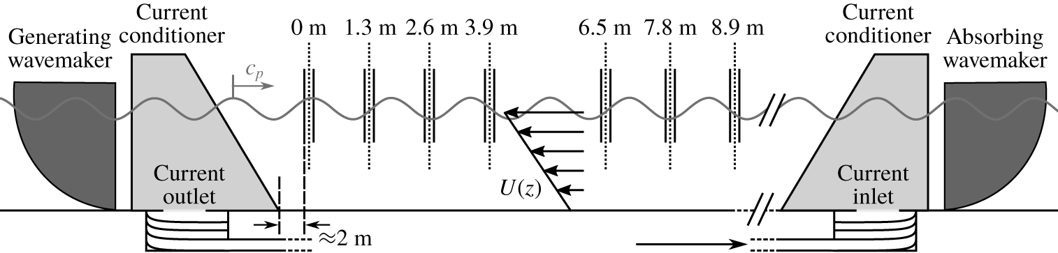
Schematic diagram illustrating the wave–current flume at UCL configured for a typical case of currents (with inline velocity,  $U(z)$) opposing wave phase velocity,
 $c_{p}$. Individual wave gauges are denoted by solid vertical lines. Gauges are arranged in pairs separated by
 $0.15~\text{m}$ to allow estimates of the incident and reflected free surface elevation at the mid-point of each gauge pair (denoted by the dotted vertical lines).

3 Experimental methodology
The experiments aim to determine the effect of a vertical, linearly sheared current on the frequency dispersion of low-steepness linear waves and the stability of weakly nonlinear wavetrains. To achieve this, three stages are defined: current creation, in which a suitable current profile is sought; linear dispersion (part I), in which the dispersive behaviour of linear (low-steepness) waves is measured; and, ultimately, modulational instability (part II), in which the behaviour of weakly nonlinear waves is examined.
3.1 Wave–current facility
The wave–current flume in the Department of Mechanical Engineering at University College London (UCL) is used for all experiments considered in this paper. The flume consists of a recirculating current system and two force-feedback wavemakers capable of both generation and absorption, as laid out in the facility schematic (figure 3). Current is recirculated underneath the flume by three parallel  $0.3~\text{m}$ diameter pipes and three impeller pumps, before passing through turning vanes and upwelling into the bottom of current conditioning units. The flume has width,
 $w=1.2~\text{m}$, a working depth,
 $d=0.5~\text{m}$ and wavemaker-to-wavemaker length of
 $16~\text{m}$. It should be noted that the current conditioning units limit the working length of the flume to approximately
 $9~\text{m}$. The first wave gauge defines the
 $x$-axis origin, and all horizontal distance measurements along the flume are given with reference to this point. Steel rails allow wave gauges to be fixed
 $0.3~\text{m}$ from the flume side.
Having a width of  $1.2~\text{m}$, wave energy dissipation in the facility arising from sidewall friction (the dominant source of dissipation (Hughes Reference Hughes1993)) was considered. Linear waves are known to undergo exponential amplitude attenuation due to sidewall friction; high-frequency waves being attenuated more than low-frequency waves (Hughes Reference Hughes1993). Additionally, Segur et al. (Reference Segur, Henderson, Carter, Hammack, Li, Pheiff and Socha2005) suggest that modulational instability may be entirely stabilised by any form of dissipation. Kimmoun et al. (Reference Kimmoun, Hsu, Branger, Li, Chen, Kharif, Onorato, Kelleher, Kibler and Akhmediev2016) show theoretically and experimentally that a perturbation from precise initial conditions causes a phase shift to FPUT recurrence and, in the case of the spatially localised Akhmediev breather, induces FPUT-type recurrence, where it would otherwise not occur. However, the evolution distance of our experiments did not allow for long-term recurrence effects to be observed. Using the equations presented in Hughes (Reference Hughes1993), we estimate frictional attenuation to be no more than
 $3\,\%$ along the working length of the flume. Additionally, the propagation of regular waves at
 $k=6.0~\text{rad}~\text{m}^{-1}$ (the carrier wavenumber in all experiments in part II) was recorded on each current profile, and attenuation was found to be smaller than the variation between the four repeated experiments and thus undetectable.
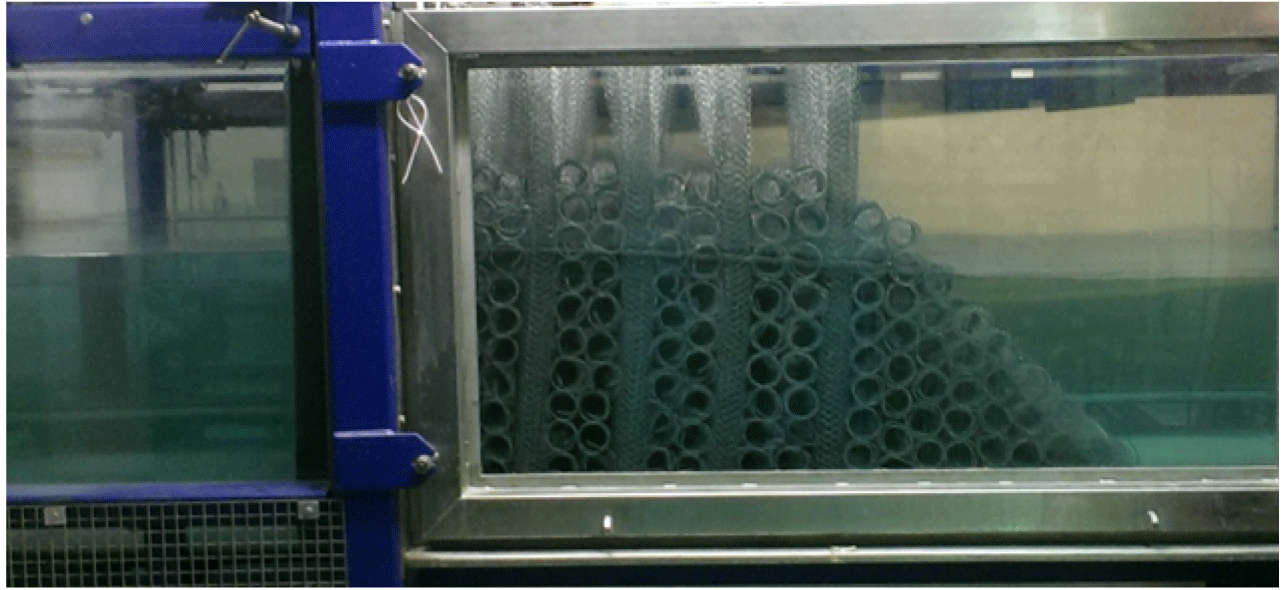
Current conditioning unit located above the outlet of the wave–current flume at the UCL Mechanical Engineering Department. Porous mesh cylinders make up the bulk conditioner (left) and triangular current shaping portion (right). The locations of the units are shown in the facility schematic of figure 3.

3.2 Current conditioning
Figure 4 shows a current conditioner positioned above the outlet turning vanes. The system of current conditioning described herein has been employed in previous experiments at the facility and is described in detail by Stagonas, Buldakov & Simons (Reference Stagonas, Buldakov, Simons and Lynett2014) and Santo et al. (Reference Santo, Taylor, Eatock and Choo2013). Each conditioning unit spans the width of the flume and consists of a rectangular bulk conditioner whose primary purpose is to reduce turbulence and distribute current evenly as it enters the flume. The rectangular unit abuts onto a triangular current-shaping unit. The bulk conditioner is constructed from porous wire mesh cylinders of diameter  ${\approx}0.1~\text{m}$. During construction, pairs of horizontal cylinders are laid transversely across the flume and additional cylinders stacked on top, the stack reaching an elevation well above the still water level. Along the flume, the stacks are separated by
 $0.1~\text{m}$ gaps in which vertical porous mesh cylinders are placed. The current-shaping unit consists of porous mesh cylinders placed horizontally across the flume and stacked to form a right-angled triangle. The current conditioners were optimised to generate current profiles which do not change considerably along the flume and have a significant linear portion.
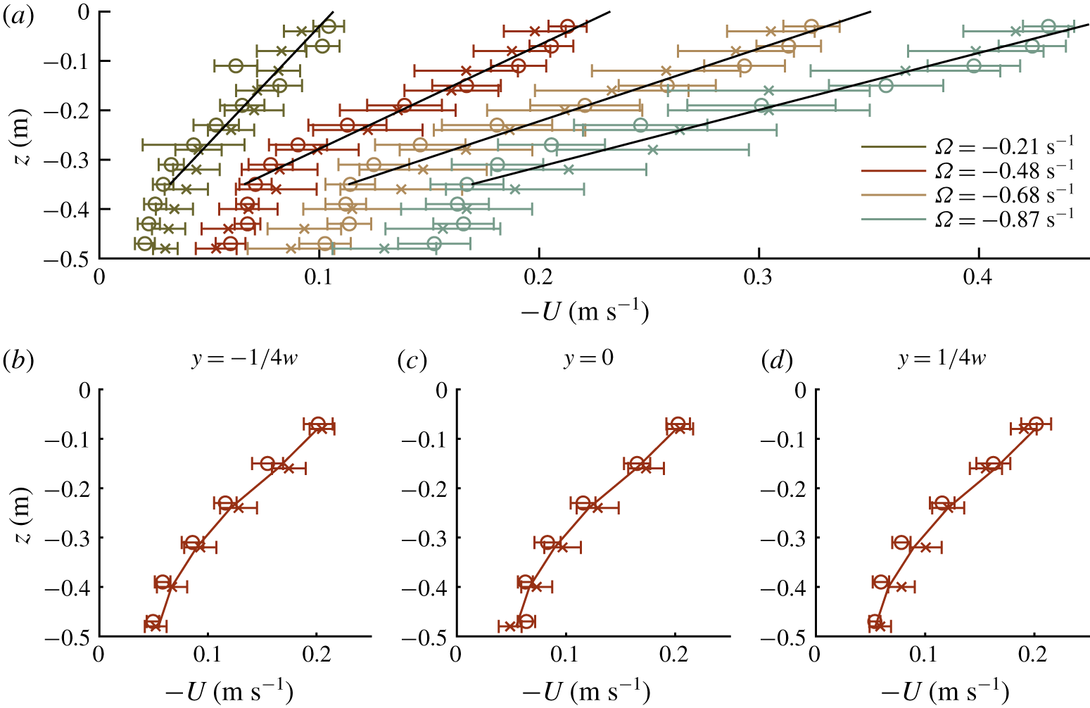
Measured current velocity profiles used in experiments presented herein. Open circles represent mean measurements taken at  $x=0~\text{m}$ and crosses at
 $x=9~\text{m}$. Error bars span one standard deviation calculated across the
 $60~\text{s}$ velocity record. (a) All non-zero velocity profiles. Solid black lines represent the linear regression used to estimate the shear rate. All measurements were taken midway across the flume (at
 $y=0~\text{m}$). (b–d) The
 $\unicode[STIX]{x1D6FA}=-0.48~\text{s}^{-1}$ current profile measured at one quarter, midway and three quarters across the width of the flume,
 $w$, namely at
 $y/w=-1/4$,
 $0$ and
 $1/4$. The (identical) solid lines correspond to the mean current profile measurement across all
 $6$ locations.

3.3 Current profile approximation
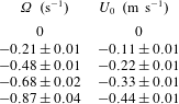
Experiments were conducted with opposing currents (with negative surface current velocity), because the effective length of evolution in the following-current case was considered too short to observe any nonlinear effects. Five current profiles were created and will be referred to herein by their shear rates,  $\unicode[STIX]{x1D6FA}$:
 $0$ (zero current),
 $-0.21$,
 $-0.48$,
 $-0.68$ and
 $-0.87~\text{s}^{-1}$. These values can be found, along with their associated surface current velocities, in table 1 where the
 $95\,\%$ confidence bounds of both parameters are also given.
Acoustic Doppler velocimetry (ADV) was used to measure the depth-varying, three-component velocity profiles at two positions defined by the coordinates,  $(x,y,z)$ along the flume centreline: at
 $(0,0,z)~\text{m}$ and at
 $(9,0,z)~\text{m}$ (with
 $y=0$ corresponding to midway across the flume). As the fastest current profile used in the stability experiments, the
 $-0.48~\text{s}^{-1}$ shear current profile was also measured at three positions across the flume to assess three-dimensional effects. Velocity measurements through the flume depth were taken from the bed in consecutive
 $0.04~\text{m}$ vertical increments to the free surface. At each position, all three velocity components,
 $(U,V,W)$, were measured at
 $200~\text{Hz}$ for one minute. Prior to each current profile change, the flume was allowed to settle for one hour to reach a steady state, at which time seeding material was added.
Figure 5 presents the mean and standard deviation values of the inline velocity,  $U$, as calculated from the full time-series data. The shear rate,
 $\unicode[STIX]{x1D6FA}$, and surface current,
 $U_{0}$, fully define the linearly varying approximation of each current profile and are presented in table 1 along with their
 $95\,\%$ upper and lower confidence bounds. The shear rate was estimated using a linear regression fit through the current’s upper, linear portion. The deeper in the fluid, the smaller the effect of the current’s velocity and shear rate on wave phase velocity (Stewart & Joy Reference Stewart and Joy1974). Excluding current data below
 $z=-0.35~\text{m}$ from the linear regression fit allows an accurate estimation of shear rate (see appendix B for a detailed estimation of the small resulting error based on the Rayleigh equation (Skop Reference Skop1987)). Surface current was estimated using a smoothing spline fitted through the entirety of the depth-varying current data.
Mean and associated  $95\,\%$ confidence bound values of surface current velocity,
 $U_{0}$ and linear shear rate,
 $\unicode[STIX]{x1D6FA}$ for the
 $5$ current profiles used in experiments.

3.4 Part I. Linear dispersion relation
By observing the relationship between frequency and wavenumber for low-steepness regular waves, experimental estimates of the vor-dispersion relation (2.4) are obtained. For all five current profiles, regular waves with input frequencies between the wavemaker’s low-frequency mechanical limit and the high-frequency wave-blocking limit ( $3.6<\unicode[STIX]{x1D714}<9.4~\text{rad}~\text{s}^{-1}$) were selected. Free surface elevation data were both recorded and displayed in real time at two gauges spaced at the estimated wavelength of the generated wave. The wave gauge pair spacing was then adjusted to bring both free surface measurements into phase, and this distance (now at precisely one wavelength) was recorded. Waves at each frequency were generated at a sufficiently low amplitude (
 $ka\ll 0.1$) to keep behaviour primarily linear. The precise frequency in the laboratory frame was extracted from the measured free surface elevation data. To remove the effect of surface current and determine the effect of shear, this measured frequency,
 $\unicode[STIX]{x1D714}$ was converted to the surface current frame through (2.2). Measured dispersion relation data were compared against vor-dispersion predictions and the zero-shear dispersion relation (see § 4.1 for discussion and figure 6 for results).
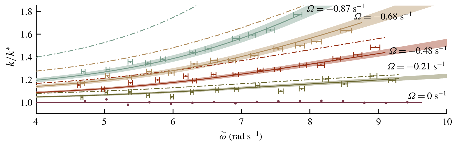
Comparison of the measured dispersion relationship (solid dots with error bars) with wavenumber predictions from the calculated vor-dispersion relationship (solid lines) and uniform-current dispersion relationship (dashed-dot lines). The wavenumbers on the  $y$-axis have been normalised by
 $k^{\ast }$, the wavenumber predicted at zero current. The horizontal error bars represent the error associated with the surface current velocity estimation (
 $95\,\%$ confidence bounds). Similarly, the shaded areas represent the error associated with the shear rate estimation (
 $95\,\%$ confidence bound).

3.5 Part II. Modulational instability
In order to examine modulational instability, a 3-component wave was created consisting of a carrier wave seeded with two sideband components, akin to the classical experiments on modulational instability without shear undertaken by Yuen & Lake (Reference Yuen and Lake1982). In particular, a medium-steepness carrier wave seeded with two symmetric sidebands was selected. The target free surface elevation given as input to the generating wavemaker was,
 $$\begin{eqnarray}\unicode[STIX]{x1D702}(0,t)=\text{Re}[a_{0}\text{e}^{-\text{i}\unicode[STIX]{x1D714}_{0}t}+a_{\unicode[STIX]{x1D6FF}}(\text{e}^{-\text{i}(\unicode[STIX]{x1D714}_{0}+\unicode[STIX]{x1D714}_{\unicode[STIX]{x1D6FF}})t}+\text{e}^{-\text{i}(\unicode[STIX]{x1D714}_{0}-\unicode[STIX]{x1D714}_{\unicode[STIX]{x1D6FF}})t})],\end{eqnarray}$$
where  $a_{\unicode[STIX]{x1D6FF}}$ and
 $\unicode[STIX]{x1D714}_{\unicode[STIX]{x1D6FF}}$ are the real sideband amplitude and arbitrary sideband frequencies respectively. To maintain a periodic signal over the repeat period,
 $R$, all frequencies were defined in terms of an integer multiple
 $N$ such that
 $f_{\unicode[STIX]{x1D6FF}}=N/R~\text{Hz}$ and
 $\unicode[STIX]{x1D714}_{\unicode[STIX]{x1D6FF}}=2\unicode[STIX]{x03C0}f_{\unicode[STIX]{x1D6FF}}~\text{rad}~\text{s}^{-1}$. For each current profile, sideband frequency was altered across experiments to explore a range of stability regimes. Sideband frequencies are given in table 3 as values of
 $N$ and are also shown, along with estimates of growth rate in figure 2. Although breather-type solutions to the NLSE would produce the most extreme amplitude growth and have been used successfully to study properties of the NLSE in the absence of shear, they require precise control of the full input signal. Such control is impeded in the present case because the waves created by the wavemaker first have to propagate onto the current (and travel through the current conditioning unit), which has a different effect on the phase and amplitude of components of different frequencies. Experimental measurements of sideband amplitude were compared with numerical solutions of the vor-NLSE and NLSE through a numerical, space-marching scheme and with predictions by linear stability analysis. The error associated with removing shear from predictions could then be quantified experimentally.
3.5.1 Data collection
To capture the evolution of the 3-component system, the free surface elevation was recorded across a total length of  $8.9~\text{m}$ by
 $14$ wave gauges arranged in
 $7$ pairs. Wave gauges collected data for a total of
 $160~\text{s}$ at
 $250~\text{Hz}$. A repeat period of
 $128~\text{s}$ was used to ensure high frequency resolution and thus allow a high number of sideband frequencies to be tested. To facilitate the application of simple reflection analysis (based on Goda & Suzuki (Reference Goda and Suzuki1976)) of the free surface elevation time series, each pair of wave gauges had a spacing of
 $0.15~\text{m}$, and produced one incident and one reflected spectrum at a virtual gauge located at each pair’s centre. Figure 3 presents the flume configuration for stability experiments where individual wave gauges are represented by solid, free surface penetrating lines and dotted lines represent virtual gauges.
Throughout the stability investigation, the same experimental procedure was followed across multiple days. Firstly, current was generated for one hour to homogenise the flume contents (for zero-current experiments, the flume was allowed to settle for a further hour thereafter). All wave gauges were wiped with a damp cloth to remove contaminants. To calibrate the wave gauges, the voltage of each wave gauge was recorded for  $30~\text{s}$ at five known free surface positions.
At each current profile, 15–17 sideband frequencies spanning nominally stable and unstable regimes were propagated with a carrier wave. Each sideband frequency experiment was carried out  $4$ times on different days. Confidence bands calculated from these
 $4$ repeats are thus indicative only. The data processing technique described below was performed on each repeat individually before a mean and standard deviation result was calculated. Between each experiment, the flume was allowed to settle for 5 minutes while reflections and low frequency error waves attenuated; current conditioners helped with this process.
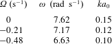
Carrier wave parameters for stability experiments (part II). All experiments were carried out at  $k_{0}=6.0~\text{rad}~\text{m}^{-1}$ and
 $k_{0}d=3.0$. The average measured steepness at each shear profile is also presented.

Sideband frequency parameters of stability experiments (part II), with completed experiments indicated by coloured cells. Frequencies are expressed as the integer multiple,  $N$, of the inverse of the repeat period,
 $R$, giving
 $f_{\unicode[STIX]{x1D6FF}}=N/R~\text{Hz}$ and
 $\unicode[STIX]{x1D714}_{\unicode[STIX]{x1D6FF}}=2\unicode[STIX]{x03C0}f_{\unicode[STIX]{x1D6FF}}~\text{rad}~\text{s}^{-1}$ (corresponding values of the perturbation wavenumber,
 $\hat{K}$, are shown in figure 2b). Repeat period,
 $R$, was fixed at
 $128~\text{s}$ across all experiments.

3.5.2 Experimental parameters
Table 2 details the carrier wave input parameters while table 3 details the sideband parameters. The primary objective when selecting the input spectra and current profiles for the stability experiments was to produce high-quality waves of medium steepness. Due to the frequency range of the wavemakers, following currents could not be considered because of the reduction in wave steepness through their interaction with waves and their small effective length of evolution, limiting experiments to negative (stabilising) shear rates. Additionally, the wave-blocking criterion,  $\unicode[STIX]{x2202}\tilde{\unicode[STIX]{x1D714}}/\unicode[STIX]{x2202}k+U_{0}\geqslant 0$ excluded the highest frequencies and current strengths. Unpredictable attenuation of waves through the current conditioning units and wave steepening by opposing currents meant that input amplitude selection was based on preliminary measurements of a range of input amplitudes.
Results from linear stability analysis of the vor-NLSE were used to inform stability experiment parameters and target the stable and unstable regions of the sideband frequency domain. To allow experimental parameters to be plotted on a single surface of linear stability (cf. figure 2), the depth parameter was kept constant at  $k_{0}d=3$ across all current profiles. Constant flume depth was maintained, and input carrier frequency altered across the three current profiles to maintain
 $k_{0}=6.0\pm 0.1~\text{rad}~\text{m}^{-1}$. The generated wavelength was checked using the method detailed in § 3.4, and the input carrier frequency adjusted if required.
3.5.3 Reflection analysis
Following the collection and calibration of wave gauge time series, the  $160~\text{s}$ free surface elevation series was cut to the final
 $128~\text{s}$ to give a periodic signal of frequency resolution
 $1/128~\text{Hz}$ containing both incident and reflected waves. Amplitude spectra were estimated from each gauge and a (linear) reflection analysis based on Goda & Suzuki (Reference Goda and Suzuki1976) applied to each gauge pair. The reflection analysis assumes that, at two closely spaced gauges (
 $\unicode[STIX]{x0394}x\ll \unicode[STIX]{x1D706}$), complex amplitude spectra,
 $A_{1}$ and
 $A_{2}$, are comprised of incident,
 $A_{I}$, and reflected,
 $A_{R}$, components,
 $$\begin{eqnarray}A_{1}=A_{I}\text{e}^{-\text{i}k_{I}\unicode[STIX]{x0394}x/2}+A_{R}\text{e}^{\text{i}k_{R}\unicode[STIX]{x0394}x/2}\quad \text{and}\quad A_{2}=A_{I}\text{e}^{\text{i}k_{I}\unicode[STIX]{x0394}x/2}+A_{R}\text{e}^{-\text{i}k_{R}\unicode[STIX]{x0394}x/2},\end{eqnarray}$$
where the incident and reflected wavenumbers,  $k_{I}$ and
 $k_{R}$, are calculated using the relevant dispersion equation (i.e. including current and shear). The method assumes linear evolution between gauges within a pair, and linear stability analysis estimates of sideband growth across the short, 0.15 m distance confirmed this assumption to be satisfactory. Our use of this technique deviates from the classical method described by Goda & Suzuki (Reference Goda and Suzuki1976) only in that we use the vor-dispersion equation (validated in § 4.1) to compute incident and reflected wavenumbers. Reflections were found to be largest in the zero current experiments where they comprised 5 %–10 % of the measured energy. This value reduced for adverse current experiments but reflection analysis was applied to all experiments regardless. All results presented include only incident waves. Following the reflection analysis, upper and lower sidebands were identified in the incident wave spectrum at the first gauge and their amplitude tracked across all seven gauge pairs.
4 Results
4.1 Part I. Linear dispersion relation
Figure 6 presents the measured results from part I in the form of measured wavenumbers as a function of frequency in the surface current reference frame. The measured wavenumbers are compared to the predictions by both the vor-dispersion equation and the classical uniform-current dispersion equation. Mean wavenumber values are represented by solid dots and error bars indicate the effect of using upper and lower surface current confidence bounds when calculating  $\tilde{\unicode[STIX]{x1D714}}$ from (2.2). The vor-dispersion prediction is delineated by solid lines surrounded by shaded areas which define the error associated with use of the upper and lower shear rate confidence bounds when calculating wavenumber from (2.4). The dot-dashed lines denote the wavenumber prediction by the uniform-current dispersion relation. Normalisation by the wavenumber for zero current is performed on all wavenumbers. This normalisation allows the fractional error associated with discounting both surface current and shear rate to be clearly appreciated.
The dispersion measurements in the absence of currents exhibit almost zero deviation from the prediction of the standard arbitrary-depth dispersion relation. The greatest error in this data set is  $2.6\,\%$ above the predicted wavenumber. At the
 $-0.21~\text{s}^{-1}$ shear rate, the zero-shear prediction begins to deviate from the vor-dispersion prediction. In general, the experimental measurements follow the trend of the vor-dispersion relation. Experimental error bars at larger frequency values (
 $\tilde{\unicode[STIX]{x1D714}}>8.0~\text{rad}~\text{s}^{-1}$) show that measurements lie within the error associated with the measurement of shear. The
 $-0.48~\text{s}^{-1}$ shear current profile presents a much larger deviation in the zero-shear prediction with respect to experimental measurements that fall almost entirely within the shaded region associated with the vor-dispersion relation. This good agreement between experimental measurements and the vor-dispersion predictions also occurs for the
 $-0.68~\text{s}^{-1}$ and
 $-0.87~\text{s}^{-1}$ shear rate current profiles.
4.2 Part II. Modulational instability
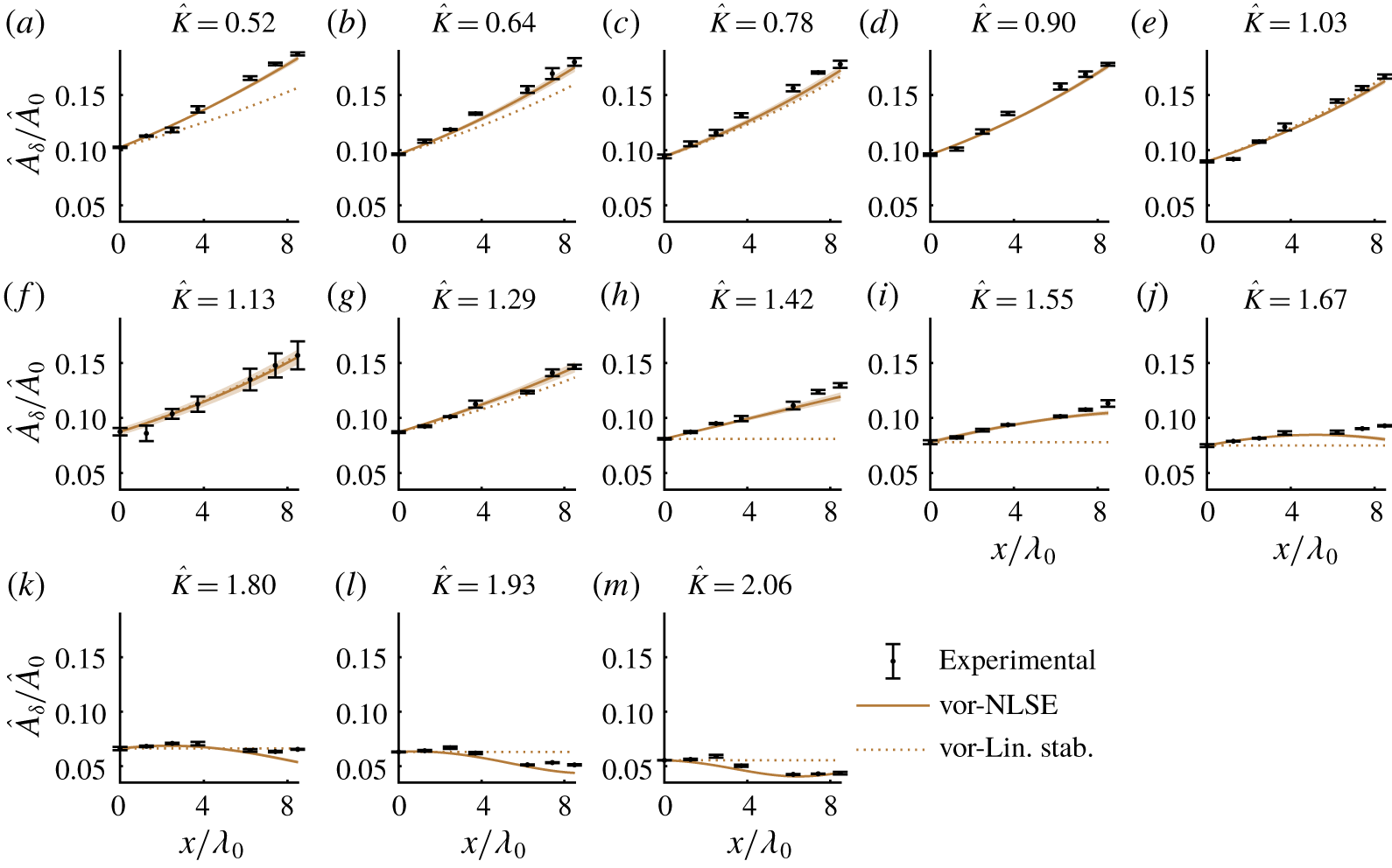
Case  $\unicode[STIX]{x1D734}=0~\text{s}^{-1}$. Combined upper and lower primary sideband Fourier amplitudes,
 $\hat{A}_{\unicode[STIX]{x1D6FF}}$ normalised by the carrier Fourier amplitude,
 $\hat{A}_{0}$. Error bars denote two standard deviations from the mean as averaged across four repeats (part II). All sideband wavenumbers are represented as the normalised sideband wavenumber parameter
 $\hat{K}=K/(a_{0}\sqrt{-M^{\ast }/L^{\ast }})$. Solid lines denote numerical predictions, while dotted line predictions are based on growth rates obtained from linear stability analysis.

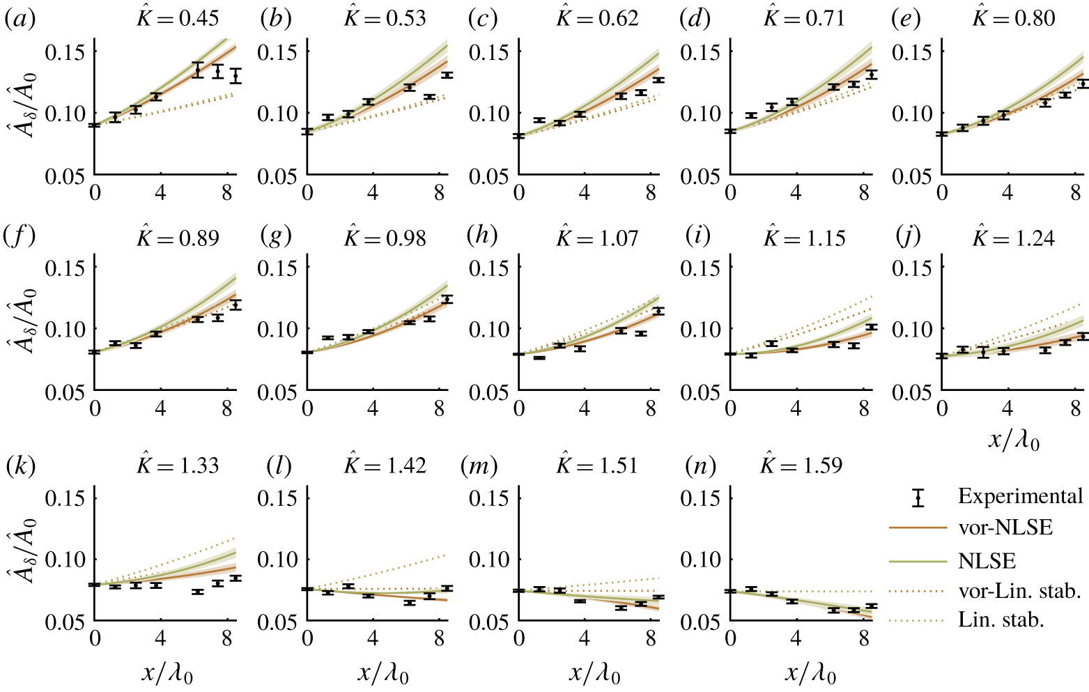
Case  $\unicode[STIX]{x1D734}=-0.21~\text{s}^{-1}$. Combined upper and lower primary sideband Fourier amplitudes,
 $\hat{A}_{\unicode[STIX]{x1D6FF}}$, normalised by the carrier Fourier amplitude,
 $\hat{A}_{0}$. Error bars denote two standard deviations from the mean as averaged across four repeats (part II). All sideband wavenumbers are represented as the normalised sideband wavenumber parameter
 $\hat{K}=K/\left(a_{0}\sqrt{-M^{\ast }/L^{\ast }}\right)$. Solid lines denote numerical predictions, while dotted line predictions are based on growth rates obtained from linear stability analysis. Brown lines delineate results obtained from the vor-NLSE whereas green lines delineate results from the uniform-current NLSE.

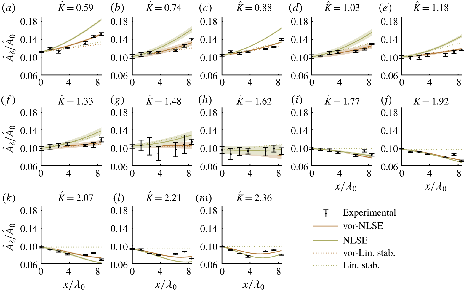
Case  $\unicode[STIX]{x1D734}=-0.48~\text{s}^{-1}$. Combined upper and lower primary sideband Fourier amplitudes,
 $\hat{A}_{\unicode[STIX]{x1D6FF}}$ normalised by the carrier Fourier amplitude,
 $\hat{A}_{0}$. Error bars denote two standard deviations from the mean as averaged across four repeats (part II). All sideband wavenumbers are represented as the normalised sideband wavenumber parameter
 $\hat{K}=K/\left(a_{0}\sqrt{-M^{\ast }/L^{\ast }}\right)$. Solid lines denote numerical predictions, while dotted line predictions are based on growth rates obtained from linear stability analysis. Brown lines delineate results obtained from the vor-NLSE whereas green lines delineate results from the uniform-current NLSE.

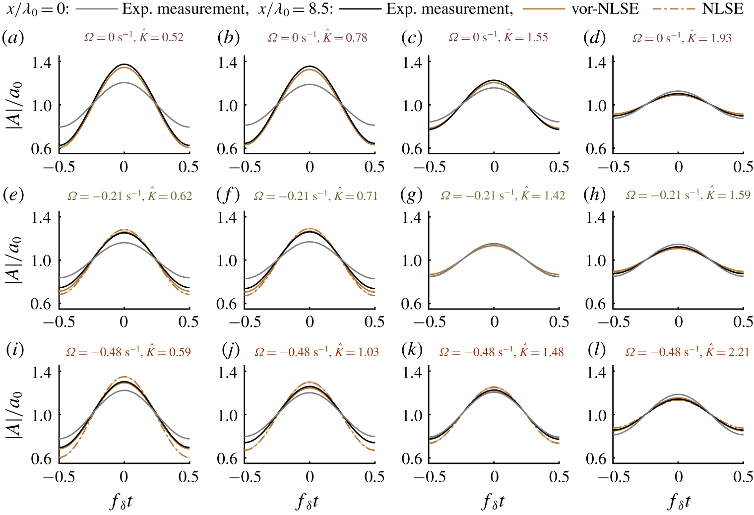
Envelopes of the linearised experimental incident wavetrains,  $A$, at
 $x=0~\text{m}$ (grey line, used as wavemaker boundary condition to numerical solution) and
 $x=8.9~\text{m}$ (black line) normalised by the carrier component amplitude and compared with predictions by the vor-NLSE (continuous brown lines) and zero-shear NLSE (dot-dashed brown lines) as a fraction of its carrier amplitude (part II).

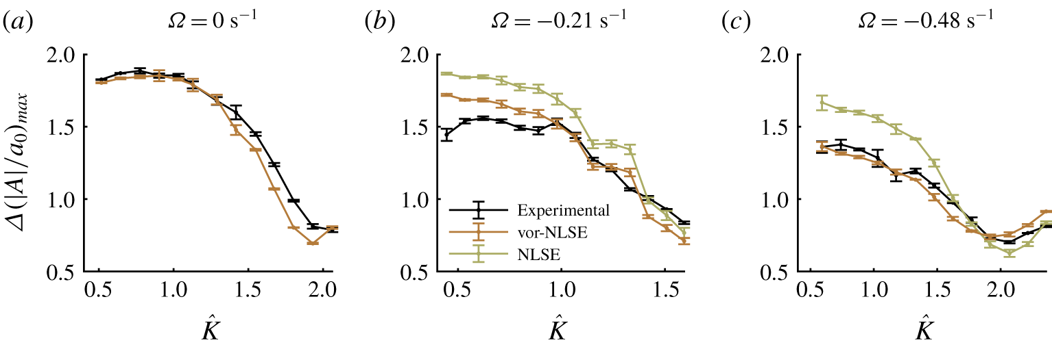
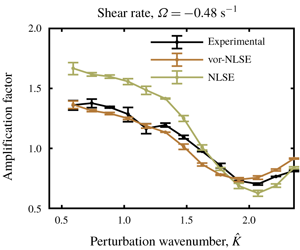
Maximum amplification factors, denoting the ratio between the maximum envelope amplitudes at the first and final gauges, as a function of the normalised sideband wavenumber parameter  $\hat{K}=K/\left(a_{0}\sqrt{-M^{\ast }/L^{\ast }}\right)$ and for the three shear rates.

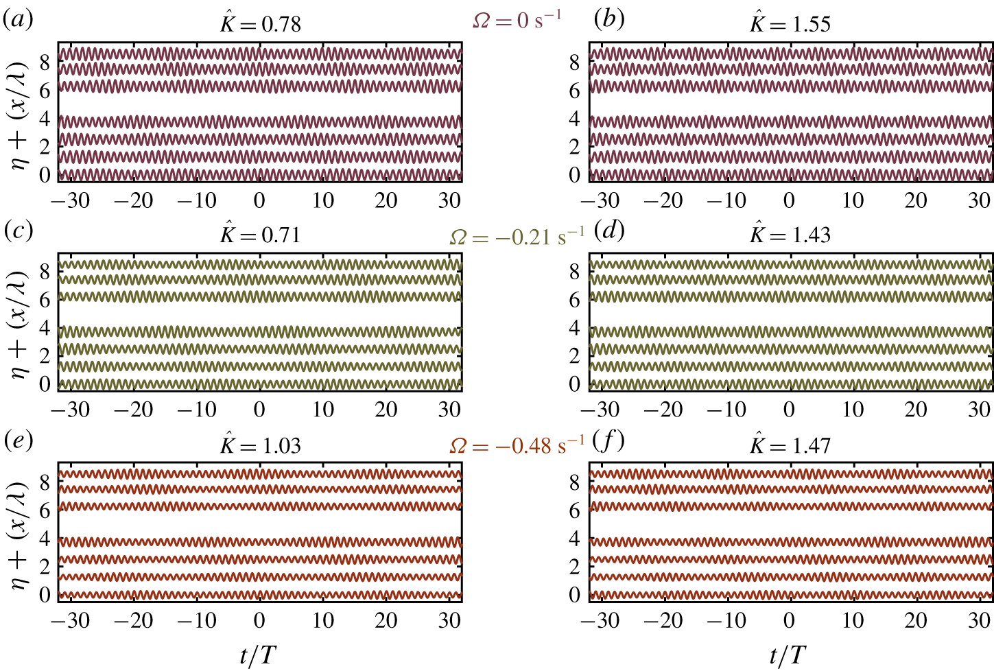
Evolution of experimental incident free surface elevation for nominally unstable (a,c,e) and marginally unstable (b,d,f) sideband frequencies (part II) for the three shear rates. A scaled free surface elevation,  $25\unicode[STIX]{x1D702}$ is presented to make plots clear. We note the gap between gauge location 4 and 5 is due to a lack of data from a faulty wave gauge (this is also evident in all other results figures).

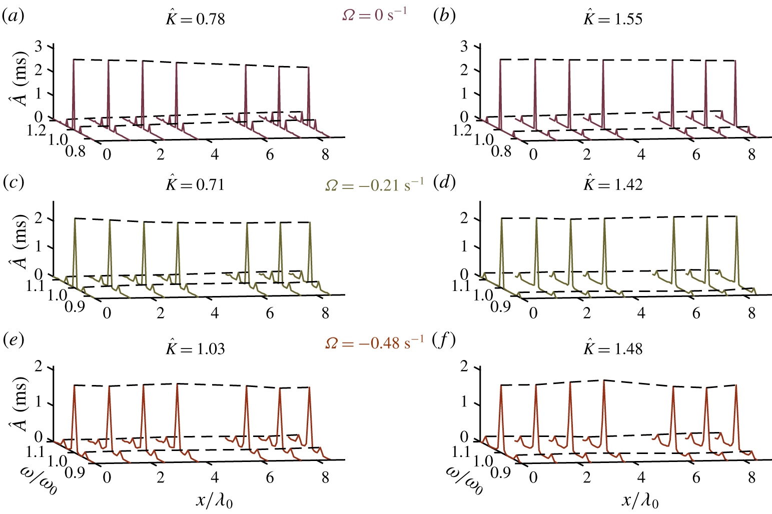
Evolution of experimental incident amplitude spectra for unstable (a,c,e) and marginally unstable (b,d,f) sideband frequencies. Black dashed lines mark the carrier and primary sideband amplitudes through their spatial evolution (part II).

Figures 7–11 present the measured and predicted evolution of the weakly nonlinear wavetrains investigated in part II. Panels within figures are titled according to the normalised perturbation wavenumber,  $\hat{K}=K/K(\tilde{\unicode[STIX]{x1D6FE}}_{max}^{\ast })$, where
 $\unicode[STIX]{x1D6FE}_{max}^{\ast }$ is the maximum growth rate evaluated at
 $k_{0}d=3$ and zero shear (i.e.
 $\hat{K}=1$ at the zero-shear maximum growth rate). Normalised perturbation wavenumbers allow results to be directly related to the growth rate surface in figure 2. Following reflection analysis, spectral information was extracted from incident wave spectra and is compared with the predictions of a linear stability analysis of the vor-NLSE (overview in § 2.3.3) and a space-marching numerical split-step (or pseudospectral) scheme (see Weideman & Herbst (Reference Weideman and Herbst1986) and Taha & Ablowitz (Reference Taha and Ablowitz1984) for details) that solves the same equation. Both theoretical methods allow the removal of shear from their predictions in order to quantify the error associated with ignoring vertical shear. The complex amplitudes and frequencies of sidebands and carrier waves were extracted from the incident amplitude spectrum at
 $x=0.0~\text{m}$; these were then used as initial conditions for both theoretical methods. The numerical scheme was executed for all experiment repetitions, and the average and standard deviation of sideband amplitudes calculated across these.
Figures 7–9 present the evolution of seeded sideband amplitudes in both the absence of currents and in the presence of opposing currents. Averages of the upper and lower sidebands are given normalised by the initial carrier amplitude. Due to the spectral symmetry of NLSEs, individual upper and lower sidebands are predicted less well than their averages by the vor-NLSE, but are included for completeness in appendix C. Numerical solutions of the vor-NLSE and NLSE are presented alongside experimental results. Mean amplitudes across four repeats are represented by dots (experimental) and lines (theoretical), while error bars and shaded areas represent two standard deviations from the mean for experimental and theoretical results respectively. Shaded areas are not always visible due to strong repeatability.
Figure 10 presents a sample of the evolution of incident envelopes (linearised by filtering bound waves and averaged over repeats) as measured experimentally and predicted through the NLSE and vor-NLSE numerical solutions by showing these envelopes at the first and final gauge. The ratio between maximum envelope amplitude at the final and first gauge gives an amplification factor associated with the perturbation wavenumber and shear rate; this amplification factor is presented for all experiments in figure 11. In both figures 10 and 11 the effect of shear on the formation of extreme wave crests becomes clear. Incident free surface elevation time series and associated amplitude spectra are presented in figures 12 and 13, respectively.
4.2.1 Zero current
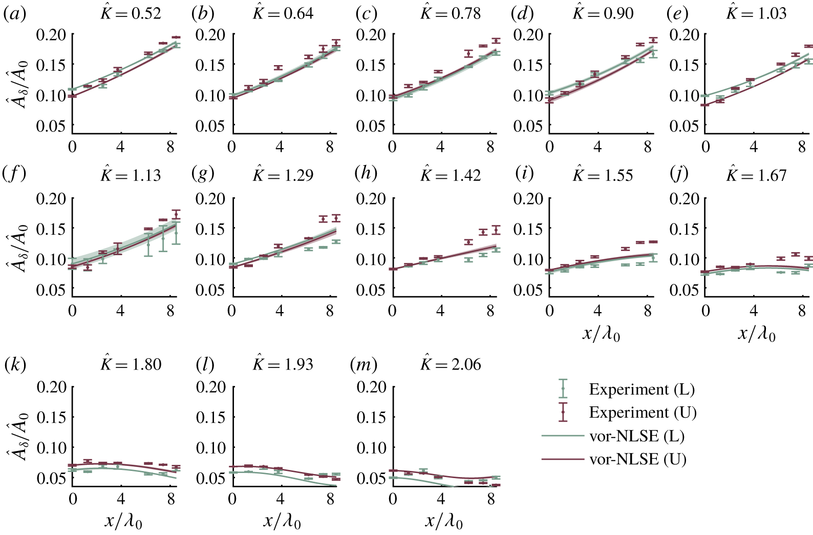
Figure 7 presents sideband evolution in the absence of current (and shear). Growth is clearly visible through the  $0.52\leqslant \hat{K}\leqslant 1.29$ sideband wavenumber range, as predicted by linear stability analysis. Here, sideband amplitudes all increase by more than
 $60\,\%$ with a maximum amplification by
 $87\,\%$ occurring at
 $\hat{K}=0.90$. We did not observe breaking in any experiments, and significant decay in sideband amplitude was never recorded, thus indicating we did not observe (the beginnings of) FPUT recurrence in our short flume. In the range
 $1.29\leqslant \hat{K}\leqslant 1.67$, sideband amplification reduces significantly, having crossed the theoretical stability boundary at
 $\hat{K}=1.42$ (beyond which sideband amplitude behaviour is expected to become oscillatory). Such oscillations are observed in both experimental measurements and the numerical solution throughout the stable region. Across all still water experiments, small error band intervals indicate that experiments were very repeatable. Numerical solutions of the NLSE exhibit very satisfactory agreement with experimental measurements over the range of still water experiments, with predictions usually falling within two standard deviations of experimental measurements.
Figure 11 shows the ratio of the maximum values of the final and first gauge envelopes presented in figure 10. In figure 11(a), the experimental amplification factors show a clear downward trend following a maximal amplification factor of approximately  $1.9$ at
 $\hat{K}=1$, the perturbation wavenumber predicted by linear stability analysis to have maximum growth at zero shear. The numerical solution to the vor-NLSE follows this trend very closely, remaining within two standard deviations throughout the unstable region (
 $\hat{K}<1.4$). Similarly, the envelopes presented in figure 10(a–d) show increases in amplitude for both unstable perturbation wavenumbers (a,b); there is good agreement between experimental and numerical results. In the stable perturbation wavenumber region (figure 10c,d), agreement between numerical and experimental envelopes is also observed.
4.2.2 Opposing currents
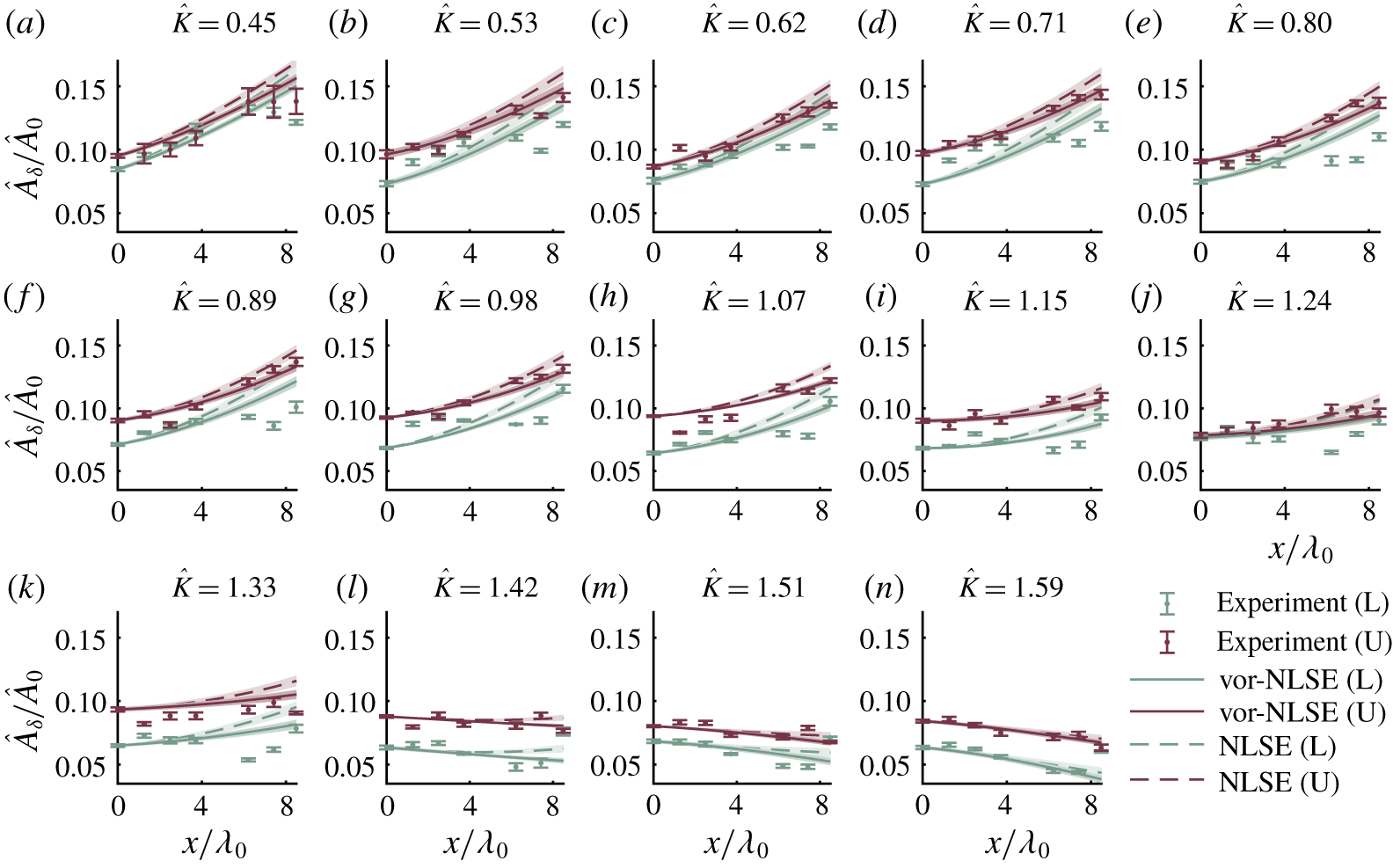
In figure 8, which illustrates the sideband evolution in  $-0.21~\text{s}^{-1}$ shear rate experiments, the experimental measurements show obvious growth for perturbation wavenumbers within the range
 $0.45\leqslant \hat{K}\leqslant 0.98$. Similarly, in the
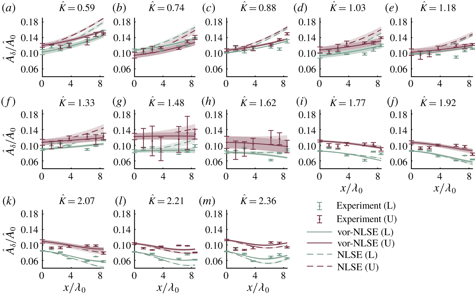
 $-0.48~\text{s}^{-1}$ shear rate experiments of figure 9, clear sideband growth is observed within the perturbation wavenumber range
 $0.59\leqslant \hat{K}\leqslant 1.03$. Maximum amplifications by
 $21\,\%$ were observed at
 $\hat{K}=0.71$ and
 $\hat{K}=0.59$ for the
 $-0.21~\text{s}^{-1}$ and
 $-0.48~\text{s}^{-1}$ shear rates respectively. Growths observed in the
 $-0.48~\text{s}^{-1}$ shear experiments are predominantly lower than in the
 $-0.21~\text{s}^{-1}$ shear case due to the carrier wave having lower steepness. As the perturbation wavenumber is increased beyond the theoretical stability threshold, both current profiles exhibit stabilisation of sideband amplitudes, with zero or negative amplification beyond
 $\hat{K}\approx 1.4$.
The numerical solutions of the vor-NLSE closely match the experimental data for both current profiles. In the  $-0.21~\text{s}^{-1}$ shear case, although removing shear from theoretical predictions leads to over-prediction of sideband growth for all unstable cases, this does not become significant until the edge of the stability region (
 $\hat{K}=1.42$) is reached. However, significant changes in sideband evolution are apparent in the
 $-0.48~\text{s}^{-1}$ shear rate case where the NLSE consistently over-predicts the amplification of sideband amplitudes at all unstable perturbation wavenumbers. This maximum error occurs predominantly at lower perturbation wavenumbers (
 $0.59\leqslant \hat{K}\leqslant 1.33$). At
 $\hat{K}=0.59$, the over-prediction exceeds
 $100\,\%$ of the measured value. Predictions from the vor-NLSE numerical scheme closely follow the sideband evolution trend well into the stable perturbation wavenumber region. In the
 $-0.48~\text{s}^{-1}$ shear rate case, above
 $\hat{K}=1.62$ the vor-NLSE predictions are still in good agreement with experimental measurements, however the vor-NLSE and NLSE results are almost indistinguishable.
The effect of discounting shear on wave height is illustrated by the linearised envelope time-series data presented in figure 10 where the over-prediction of the envelope amplitude of  $29\,\%$ in panel (i) (
 $\hat{K}=0.59$) by the NLSE is in stark contrast to the corresponding vor-NLSE result which follows the experimental measurement to an error within two standard deviations (seen as an overlap in vor-NLSE and experimental boundaries). The incorrect prediction in envelope amplitude by the NLSE in figure 10 occurs at all unstable perturbation wavenumbers of the
 $-0.48~\text{s}^{-1}$ shear current case, displaying an over-prediction of
 $16\,\%$ in the
 $\hat{K}=1.03$ (panel (j)); again the vor-NLSE results compare favourably, with an under-prediction of only
 $7\,\%$.
Figure 11 shows this significant difference in predictions between the vor-NLSE and uniform velocity NLSE occurs in all of the unstable perturbation wavenumbers at the  $\unicode[STIX]{x1D6FA}=-0.48~\text{s}^{-1}$ shear rates. As with the zero-current cases, the majority of vor-NLSE amplification factor predictions fall within two standard deviations across repeats.
Across all perturbation wavenumbers, repeatability appears to be very good with minimal changes in sideband amplitude across repeats. However, in the  $-0.48~\text{s}^{-1}$ shear case, when perturbation wavenumber approaches the stability boundary, a larger standard deviation is seen. The perturbation wavenumbers at which larger deviations exist emphasise the sensitivity of the system to initial conditions. At the very sharp perturbation wavenumber stability boundary, this nonlinear system becomes very sensitive to initial conditions where slight changes in carrier amplitude may push the system into a region of stability or instability (see appendix C).
5 Conclusion
Measurements of physical experiments have been compared with the linear and weakly nonlinear constant vorticity, arbitrary depth, linear shear wave evolution equations derived by Thomas, Kharif and Manna (Thomas et al. Reference Thomas, Kharif and Manna2012) (TKM12). It has been shown that in cases of shear  $\unicode[STIX]{x1D6FA}<-0.21~\text{s}^{-1}$ (i.e. for shear rates sufficiently large in magnitude), the constant vorticity equations consistently perform significantly better than the standard, uniform-current equations. The linear vor-dispersion equation gave results that remained within experimental error (part I). Sideband evolution predictions of the vor-NLSE consistently remained within two standard deviations across experiment repeats (part II).
In part I, the wavelengths and frequencies of low-steepness, regular waves were measured for five opposing current profiles (down to  $\unicode[STIX]{x1D6FA}=-0.87~\text{s}^{-1}$), and measured dispersion relations obtained. The experimental measurements were compared with predictions from arbitrary depth, constant vorticity and standard, uniform-current dispersion relations. For all current profiles, results from the constant vorticity dispersion relation agreed with physical measurements, where the experimental data points fell within
 $95\,\%$ confidence bounds associated with the estimation of current shear and surface current. For
 $\unicode[STIX]{x1D6FA}\leqslant -0.48~\text{s}^{-1}$, the predictions by the uniform-current dispersion relation deviated significantly from both the vor-dispersion equation and experimental measurements.
In part II, in nonlinear experiments, the sidebands of modulated wavetrains were observed to grow, creating large amplitude wave pulses and indicating modulational instability in all current profiles within the unstable perturbation wavenumber region (as predicted by linear stability analysis of the vor-NLSE). Experimental measurements of sideband amplitude were compared with numerical predictions of space-marching solvers of the vor-NLSE and the standard uniform-current NLSE. The vor-NLSE results provided a very good match to experimental measurements over the range of current profiles considered, unlike the uniform velocity NLSE whose sideband amplification predictions were consistently 10 %–30 % higher than measured.
Future work should include an investigation into the destabilising effects of positive shear. This likely requires the use of a high-velocity wave-following surface current, which is known to reduce amplitudes and thus their associated nonlinear effects. As such, wavemakers capable of high frequencies ( $\unicode[STIX]{x1D714}_{0}>12~\text{rad}~\text{s}^{-1}$) and a long evolution distance would be required. A reduction in shear rate close to the surface may also be induced by wave–current interactions (as studied in Groeneweg & Klopman (Reference Groeneweg and Klopman1998)), leading to a reduction in the effect of shear on wave stability not considered here. Additionally, the propagation of breather-type NLSE solutions (having known and previously verified amplification factors on still water) on negatively sheared currents would help to quantify the effect of a sheared current on their amplification factor, although their experimental generation will most likely rely on an iterative experimental procedure.
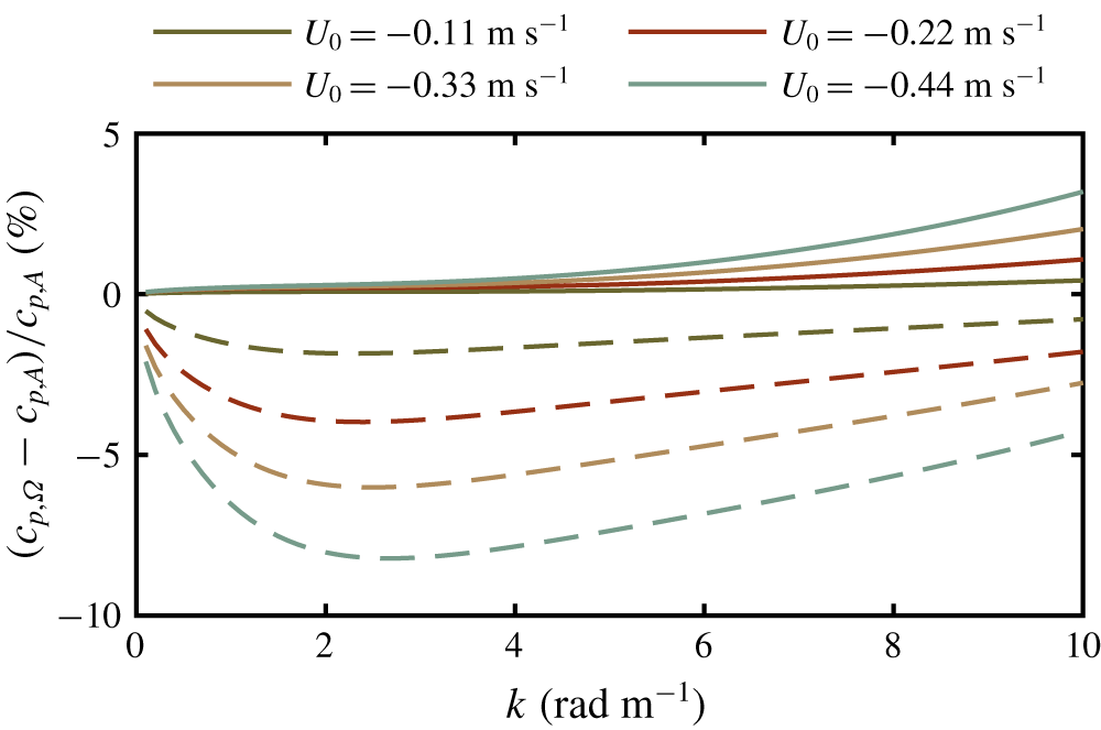
Percentage difference between the linear phase velocity calculated when assuming a linearly sheared current profile,  $c_{p,\unicode[STIX]{x1D6FA}}$, and when assuming an arbitrarily sheared current profile,
 $c_{p,A}$, for the four current profiles in table 1. The continuous lines show the effect of the linear current approximation. The dashed lines show the effect of ignoring the current’s shear altogether.

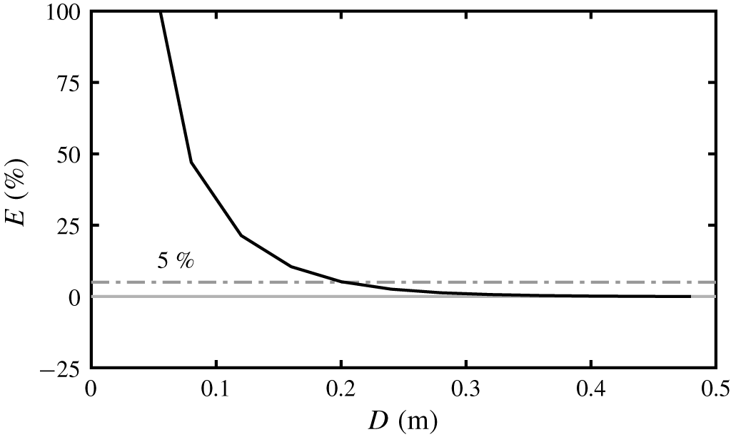
Percentage error in phase velocity associated with estimating current down to a depth,  $D$ for a wave of wavenumber,
 $k=6~\text{rad}~\text{m}^{-1}$ and the strongest shear rate (
 $\unicode[STIX]{x1D6FA}=-0.87~\text{s}^{-1}$).

Case  $\unicode[STIX]{x1D734}=0~\text{s}^{-1}$. Upper (U) and lower (L) primary sideband Fourier amplitudes,
 $\hat{A}_{\unicode[STIX]{x1D6FF}}$ normalised by the carrier Fourier amplitude,
 $\hat{A}_{0}$. Error bars denote two standard deviations from the mean as averaged across four repeats. All sidebands are represented as the normalised sideband wavenumber parameter
 $\hat{K}=K/K(\tilde{\unicode[STIX]{x1D6FE}}_{max})$.

Case  $\unicode[STIX]{x1D734}=-0.21~\text{s}^{-1}$. Upper (U) and lower (L) primary sideband Fourier amplitudes,
 $\hat{A}_{\unicode[STIX]{x1D6FF}}$ normalised by the carrier Fourier amplitude,
 $\hat{A}_{0}$. Error bars denote two standard deviations from the mean as averaged across four repeats. All sidebands are represented as the normalised sideband wavenumber parameter
 $\hat{K}=K/K(\tilde{\unicode[STIX]{x1D6FE}}_{max})$. Solid lines indicate predictions made with the constant vorticity equations while dashed lines include only surface current in their predictions.

Case  $\unicode[STIX]{x1D734}=-0.48~\text{s}^{-1}$. Upper (U) and lower (L) primary sideband Fourier amplitudes,
 $\hat{A}_{\unicode[STIX]{x1D6FF}}$ normalised by the carrier Fourier amplitude,
 $\hat{A}_{0}$. Error bars denote two standard deviations from the mean as averaged across four repeats. All sidebands are represented as the normalised sideband wavenumber parameter
 $\hat{K}=K/K(\tilde{\unicode[STIX]{x1D6FE}}_{max})$. Solid lines indicate predictions made with the constant vorticity equations while dashed lines include only surface current in their predictions.

Acknowledgements
The authors thank Mr L. Ansdell for technical assistance during experiments. J.N.S. acknowledges an EPSRC studentship (No. 1770088), and T.S.vdB. a Royal Academy of Engineering Research Fellowship.
Declaration of interests
The authors report no conflict of interest.
Appendix A. Nonlinear Schrödinger equation: arbitrary-depth coefficients
The arbitrary-depth coefficients of the constant vorticity nonlinear Schrödinger equation (vor-NLSE) were first derived by Thomas, Kharif & Manna (Reference Thomas, Kharif and Manna2012) (TKM12). For completeness, we present here the same coefficients as in TKM12. Firstly, as in TKM12, some recurring terms are defined,
 $$\begin{eqnarray}\unicode[STIX]{x1D707}=k_{0}d,\quad \unicode[STIX]{x1D70E}=\tanh \unicode[STIX]{x1D707},\quad X=\unicode[STIX]{x1D70E}\bar{\unicode[STIX]{x1D6FA}},\quad \text{and}\quad \bar{\unicode[STIX]{x1D6FA}}=\unicode[STIX]{x1D6FA}/\tilde{\unicode[STIX]{x1D714}}_{0},\end{eqnarray}$$
where  $k_{0}$ and
 $\tilde{\unicode[STIX]{x1D714}}_{0}$ are the carrier wavenumber and carrier frequency,
 $d$ is the depth and
 $\unicode[STIX]{x1D6FA}$ is the shear rate. Tilde notation specifies a property measured in the surface current reference frame (see figure 1 for details of reference frames used). The vor-NLSE takes the form,
 $$\begin{eqnarray}iA_{\unicode[STIX]{x1D70F}}+LA_{\unicode[STIX]{x1D709}\unicode[STIX]{x1D709}}-M|A|^{2}A=0,\end{eqnarray}$$
with slow-scale coordinates,
 $$\begin{eqnarray}\unicode[STIX]{x1D709}=\unicode[STIX]{x1D716}(\tilde{x}-\tilde{c}_{g}t)\quad \text{and}\quad \unicode[STIX]{x1D70F}=\unicode[STIX]{x1D716}^{2}t,\end{eqnarray}$$
and fast-scale coordinates,  $x$ and
 $t$, where
 $\unicode[STIX]{x1D716}=k_{0}a_{0}$ is the steepness of the carrier wave, and phase and group velocities are (respectively),
 $$\begin{eqnarray}\tilde{c}_{p}=\frac{\tilde{\unicode[STIX]{x1D714}}_{0}}{k_{0}},\quad \tilde{c}_{g}=\frac{\tilde{c}_{p}}{\unicode[STIX]{x1D70E}}\frac{(1-\unicode[STIX]{x1D70E}^{2})k_{0}d+\unicode[STIX]{x1D70E}(1+X)}{2+X},\quad \text{with }\unicode[STIX]{x1D70C}=\frac{\tilde{c}_{g}}{\tilde{c}_{p}}.\end{eqnarray}$$
The arbitrary-depth linear vor-NLSE coefficient is,
 $$\begin{eqnarray}L=\frac{\tilde{\unicode[STIX]{x1D714}}_{0}}{k_{0}^{2}\unicode[STIX]{x1D70E}(2+X)}\left\{\unicode[STIX]{x1D707}(1-\unicode[STIX]{x1D70E}^{2})[1-\unicode[STIX]{x1D707}\unicode[STIX]{x1D70E}+(1-\unicode[STIX]{x1D70C})X]-\unicode[STIX]{x1D70E}\unicode[STIX]{x1D70C}^{2}\right\},\end{eqnarray}$$
where we have added in the outside parentheses accidentally omitted in TKM12 (their (48)). The nonlinear coefficient is,
 $$\begin{eqnarray}M=\frac{\tilde{\unicode[STIX]{x1D714}}_{0}k_{0}^{2}(U+VW)}{8(1+X)(2+X)\unicode[STIX]{x1D70E}^{4}},\end{eqnarray}$$
where,
 $$\begin{eqnarray}\displaystyle U & = & \displaystyle 9-12\unicode[STIX]{x1D70E}^{2}+13\unicode[STIX]{x1D70E}^{4}-2\unicode[STIX]{x1D70E}^{6}+(27-18\unicode[STIX]{x1D70E}^{2}+15\unicode[STIX]{x1D70E}^{4})X+(33-3\unicode[STIX]{x1D70E}^{2}+4\unicode[STIX]{x1D70E}^{4})X^{2}\nonumber\\ \displaystyle & & \displaystyle +\,(21+5\unicode[STIX]{x1D70E}^{2})X^{3}+(7+2\unicode[STIX]{x1D70E}^{2})X^{4}+X^{5},\end{eqnarray}$$
 $$\begin{eqnarray}\displaystyle V & = & \displaystyle (1+X)^{2}(1+\unicode[STIX]{x1D70C}+\unicode[STIX]{x1D707}\bar{\unicode[STIX]{x1D6FA}})+1+X-\unicode[STIX]{x1D70C}\unicode[STIX]{x1D70E}^{2}-\unicode[STIX]{x1D707}\unicode[STIX]{x1D70E}X,\quad \text{and}\end{eqnarray}$$
 $$\begin{eqnarray}\displaystyle W & = & \displaystyle 2\unicode[STIX]{x1D70E}^{3}\frac{(1+X)(2+X)+\unicode[STIX]{x1D70C}(1-\unicode[STIX]{x1D70E}^{2})}{\unicode[STIX]{x1D70E}\unicode[STIX]{x1D70C}(\unicode[STIX]{x1D70C}+\unicode[STIX]{x1D707}\bar{\unicode[STIX]{x1D6FA}})-\unicode[STIX]{x1D707}(1+X)}.\end{eqnarray}$$
Appendix B. Current profile approximation
Although a perfectly linear profile could not be obtained, the current profiles used throughout experiments were designed to contain a strongly sheared, linearly varying velocity profile in their upper portion. The final current profiles were then investigated for their linearity using a comparison of the linear wave phase velocity predicted by a linearly sheared current,  $c_{p,\unicode[STIX]{x1D6FA}}$ and the linear wave phase velocity predicted by an arbitrarily sheared current,
 $c_{p,A}$. A perfectly linearly varying current would produce no error between these two phase velocities. Wave phase velocity,
 $c_{p}=\unicode[STIX]{x1D714}/k$, is calculated using the depth-averaged velocity,
 $\bar{U}$ in the Doppler shift equation,
 $$\begin{eqnarray}\unicode[STIX]{x1D714}=\tilde{\unicode[STIX]{x1D714}}(k)+k\bar{U},\end{eqnarray}$$
where the depth-averaged velocity  $\bar{U}$ is calculated from the Rayleigh equation (inviscid Orr–Sommerfeld equation) in finite depth (Skop Reference Skop1987) (see Stewart & Joy (Reference Stewart and Joy1974) for deep water),
 $$\begin{eqnarray}\bar{U}=\frac{2k}{1-\text{e}^{-4kd}}\left[\int _{-d}^{0}U(z)\text{e}^{2kz}\,\text{d}z+\text{e}^{-4kd}\int _{-d}^{0}U(z)\text{e}^{-2kz}\,\text{d}z\right].\end{eqnarray}$$
Equations (B 1) and (B 2) are used to calculate the percentage difference between the two phase velocities given in figure 14. At the carrier wavenumber used for all experiments in part II ( $6~\text{rad}~\text{m}^{-1}$), the error in linear wave phase velocity associated with assuming a linear current is expected to be no more than
 $1\,\%$ for the strongest current profile.
Stewart & Joy (Reference Stewart and Joy1974) also present the error,  $E$, in phase velocity associated with limiting the depth-averaged integral to a depth,
 $D$. For deep water, the depth-averaged velocity is evaluated through the depths
 $-\infty <z<-D~\text{m}$ and
 $-D<z<0~\text{m}$, and the ratio of these integrals calculated. Using the finite-depth depth-averaged velocity (B 2), we calculate this error for
 $k=6~\text{rad}~\text{m}^{-1}$ and present it in figure 15. In this figure, we only show the strongest shear, as the other shear rates gave indistinguishable results. At
 $D\geqslant 0.2~\text{m}$, the error in phase velocity is less than
 $5\,\%$, with this reducing further to less than
 $1\,\%$ at our chosen cutoff depth of
 $0.35~\text{m}$.