To FE or not to FE?

Since the Dirty Pool symposium—a special issue on panel data estimation in International Organization—addressed the topic of fixed effects models more than a decade ago, little progress has been made on the problem of unobserved unit heterogeneity in rare-event binary time-series cross-sectional (re-BTSCS) data. While at the time, this debate helped to clarify many of the issues raised by various strategies for estimating models with these data (notably the summary from King Reference King2001), the lasting legacy has been one of confusion rather than clarity. The inability of these scholars to reach a consensus leaves applied researchers unclear as to which approach they should adopt. While strategies for panel and TSCS estimation have the received renewed attention of late (Bell and Jones Reference Bell and Jones2015; Clark and Linzer Reference Clark and Linzer2015), little of this work focuses on the unique problems posed by rare event binary TSCS data. We aim to advance this discussion, revisiting the debate on unit heterogeneity in re-BTSCS data and proposing a novel fixed effects estimation strategy for such data.

When analyzing re-BTSCS data researchers often select between pooling, random effects, and fixed effects models. Most opt for either pooling, which assumes no unobserved unit heterogeneity, or random effects, which assumes that any unit heterogeneity is orthogonal to the explanatory variables. Researchers often prefer these models to fixed effects estimation even when explicitly noting that these assumptions are violated (Nel and Righarts Reference Nel and Righarts2008; Wright Reference Wright2009). While the orthogonality of predictors and unit effects is likely specious in most macro-level studies of comparative politics and international relations, these modeling strategies dominate because—drawing upon Beck and Katz (Reference Beck and Katz2001)—many adopt the view that it is never a good idea to estimate fixed effects models with re-BTSCS data.

In general, three reasons are given by researchers for avoiding fixed effects models. First, fixed effects estimation is assumed to be problematic because the unconditional estimator (i.e., unit dummy variables) suffers from the incidental parameters problem—generating biased estimates when T is small.Footnote ¹ Second, researchers are unable to recover effect estimates of time-invariant predictors.Footnote ² Finally, with rare events data, many units do not experience the event in small samples.Footnote ³ As a consequence, there is no overlap between the fixed effects and the outcome (i.e., separation), and these units do not enter the log-likelihood. That is, parameter estimates are produced using only the data from the event-experiencing set of units.

It is this final issue which seemed to most divide the participants of the Dirty Pool symposium and is the focus of our article, namely, what are the consequences of this sample selection and how should researchers proceed in light of it? We clarify that the primary consequence of this sample selection is not biased or inefficient estimates of predictor coefficients, but instead an inaccurate estimate of the baseline event risk (i.e., the unit effects).Footnote ⁴ Analyzing event-experiencing units alone produces an inflated average estimate of the event risk, as no-event units have a lower event probability than event-experiencing units on average. This, in turn, biases the marginal effect estimates of the predictors which are, in part, a function of these probabilities. This is the fundamental problem for most researchers with rare events BTSCS data: random effects is a biased estimator given non-zero correlation between predictors and unit effects, yet fixed effects estimators induce sample selection and resultant biases in marginal effects.

As a solution, we present an alternative estimation strategy for fixed effects which does not have this limitation. Our proposed penalized maximum likelihood fixed effects (PML-FE) estimator includes unit dummies, as in unconditional fixed effects, but retains the units that do not experience a rare event in the sample using a modified score function. In short, we recognize that this issue is a special case of separation and use a familiar strategy (i.e., Firth’s logit) to address it. This is predicated on the theoretical belief that all units in the sample would, in time (i.e., with enough measures), experience the outcome. Modifying the score function to reflect this penalizes the fixed effect on no-event units away from negative infinity, retaining them in the log-likelihood. Our simulations show that this allows PML-FE to outperform pooled, random effects, and unconditional fixed effects in recovering marginal effect estimates when predictors and unit effects are correlated.

Rare events and fixed effects

To fix terms, consider the familiar latent-variable representation of BTSCS as

(1)$$\eqalignno{ & y_{{it}}^{{\asterisk}} {\equals}\alpha _{i} {\plus}{\bf x}_{{{\bf it}}} \bibeta {\plus}{\epsilon}_{{it}} , \cr & y_{{it}}^{{\asterisk}} {\equals}1(y_{{it}}^{{\asterisk}} \,\gt\,0), $$

where y _it is an observed binary outcome for unit i=1,...,N at time t=1,...,T, x_it is a vector of observed explanatory variables, α _i is an unobserved unit effect, and ε _it is an i.i.d. error. Assume, as most applied researchers have, that ε _it is distributed logistic, producing

(2) $$\Pr (y_{{it}} {\equals}1\left| {\alpha _{i} ,{\bf x}_{{{\bf it}}} } \right.){\equals}{1 \over {1{\plus}{\rm e}^{{{\minus}(\alpha _{i} {\plus}\bibeta {\bf x}_{{{\bf it}}} )}},$$

with different assumptions about α _i giving rise to the familiar pooled, random effects, and fixed effects models. In short, when a researcher assumes that α _i is α for all units i—that is, there is no heterogeneity in the unit intercepts—then the pooled model is supported and (a simplified version of) Equation 2 is estimated as in standard logistic regression.

However, when α _i is believed to vary across units, one of the panel models—random or fixed effects—should offer a better fit to the data. The main criterion usually considered when selecting between random and fixed effects is whether α _i is orthogonal to x _it .Footnote ⁵ If yes, then the random effects model is often preferred.Footnote ⁶ First, it is more efficient than the fixed effects model, thereby producing smaller standard errors and superior estimates (assuming unbiasedness). Second, with random effects estimation the within-unit variance of the predictors is not partialed out, as with fixed effects, allowing researchers to obtain estimates on time-invariant predictors.

Where one assumes instead that α _i and x _it are correlated, then a fixed effects model is often more appropriate, as both pooled and random effects estimators will be biased. For logistic models, there are two fixed effects estimators: unconditional and conditional fixed effects. The former, unconditional fixed effects, includes dummy variables for each unit (except one) into the specification and maximizes the standard logit log-likelihood. The latter, conditional fixed effects, due to Chamberlain (Reference Chamberlain1980) concentrates out the fixed effects (via Σ _t y _it ) and maximizes a conditional log-likelihood function:

$$L^{C} {\equals}\Sigma _{i} ln\left( {{{{\rm exp}(\beta '\Sigma _{t} x_{{it}} y_{{it}} )} \over {\Sigma _{{d\inD_{i} }} \,{\rm exp}(\beta '\Sigma _{t} x_{{it}} d_{t} )}}} \right)$$

where d _i ={d=(d ₁,...,d _T )|d _t =0 or 1 and Σ _t d _t =Σ _t y _it }, that is, the individual combination of observed y’s for each unit i.

While conditional fixed effects is often preferred due to concerns about the incidental parameters problem, there are several limitations.Footnote ⁷ First, it does not provide estimates of the individual unit effects so we are unable to estimate substantive quantities of interest such as marginal effects or first differences. Second, it is not currently possible to estimate the coefficients of time-invariant explanatory variables, as they are indistinguishable from the invariant unit-effect. Third, those units which do not realize an event in the sample are dropped from the analysis.

It is the final issue that is the main focus of our discussion and seemed to most divide the participants of the Dirty Pool symposium—arguably between those who prefer a more cautious approach to causal inference from observational data (Green et al. Reference Green, Kim and Yoon2001), even when a significant portion of the data exhibits no within-unit variation, and those who prefer a more theoretically driven interpretation of all of the empirical evidence (Beck and Katz Reference Beck and Katz2001; Oneal and Russett Reference Oneal and Russett2001). The latter group emphasizes that dummy variables are atheoretical and remove all the between-unit variation in the data. Their reaction to Green et al. (Reference Green, Kim and Yoon2001) was particularly strong, claiming that fixed effects models are rarely, if ever, justified in the case of binary dependent variables.

In part because of the veracity of the claims made by Beck and Katz (Reference Beck and Katz2001), researchers frequently eschew fixed effects. For example, Nel and Righarts (Reference Nel and Righarts2008) write:

Similarly, in research on democratization, Wright (Reference Wright2009) argues that:

It is repeated claims such as these which give us cause for concern. Erroneously assuming that the unit effects are absent or orthogonal to the included regressors in estimation, especially when one suspects these assumptions are problematic, risks bias. Estimating a random effects model is not a stand-in for a fixed effects, it is an alternative estimation strategy dependent on a fundamentally different assumption.

Moreover, researchers often seem unclear as to why sample censoring is a concern at all. While the loss of a large proportion of one’s sample is displeasing, the particular consequences of this are rarely discussed. First, as noted by Heckman (Reference Heckman1981) this is a small sample bias given that “as T→∞ this problem becomes unimportant.” Asymptotics aside, naïve probability suggests that the extent of sample censoring should lessen with increases in time, as more units experience the event. Second, even in small sample analysis, the sample selection does not induce bias in the coefficient estimates on predictors.Footnote ⁸ The coefficient is now the within-unit effect of the predictor, for which only units with variation in the outcome provide information. Instead, it is those estimators that retain the complete sample yet fail to partial out the endogenous between-unit component of the predictors—that is, pooled and random effects—that risk bias in these coefficients.

This is not to say, however, that sample selection is without consequence, as it biases summary estimates of the base rate of the event. In short, by only retaining event-experiencing units, we overestimate the unconditional probability of the outcome.Footnote ⁹ This can be easily seen via the law of total probability (with Z an indicator for whether the units have experienced the event):

$$\mathop{\underbrace{{\Pr (Y{\equals}1)}}}\limits_{{\scriptstyle {\rm Population} \atop \scriptstyle {\rm relationship}} }{\equals}\mathop{\underbrace{{\Pr (Y{\equals}1\,\mid\,Z{\equals}1)}}}\limits_{{\scriptstyle {\rm Uncensored} \atop \scriptstyle {\rm relationship}} }\mathop{\underbrace{{\Pr (Z{\equals}1)}}}\limits_{{\scriptstyle {\rm Probability} \atop \scriptstyle {\rm uncensored}} }{\plus}\mathop{\underbrace{{\Pr (Y{\equals}1\,\mid\,Z{\equals}0)}}}\limits_{{\scriptstyle {\rm Censored} \atop \scriptstyle {\rm relationship}} }(1{\minus}\Pr (Z{\equals}1)),$$

Given that, on average,$\Pr (Y{\equals}1\,\mid\,Z{\equals}1)\,\gt\,\Pr (Y{\equals}1\,\mid\,Z{\equals}0)$—since we have observed realizations of the outcomes for these units—we will overestimate the base rate of the event if we only evaluate this subset. This not only affects any summary estimates of the event risk but any estimands which include these as inputs, such as marginal effects. Consider, for example, the average marginal effect (AME):

(3)$${\rm AME}{\equals}{1 \over n}\mathop{\sum}\limits_{i{\equals}1}^n \Pr \left( {\widehat {Y{{{\equals}1\!\!\mid\,x_{i} }},\hat{\beta },\hat{\alpha }_{i} }}} \right){\times}\left( {1{\minus}\Pr \left( {\widehat{Y{\equals}\!{{\,1\!\!\mid\! x_{i} }},\hat{\beta },\hat{\alpha }_{i} }} \right)} \right){\times}\hat{\beta }$$

which shows that even if with an accurate${\hat{\beta }} $$, inaccurate estimates of baseline probability (a function of${\hat{\alpha }} $$) induces bias in the marginal effect estimates. More specifically, overestimating the base rate due to the sample censoring causes researchers to overestimate the AME of x.Footnote ¹⁰ In short, with rare events, overestimating the unit effect shifts the location along the sigmoidal function of the logit to the right (closer to the inflection point), such that a$\hat{\beta }$$ change now has a greater effect on the probability of obtaining ones.

Since these marginal effects are often the quantity of interest for researchers with binary outcomes, biased estimates here may be as or more problematic than biased coefficient estimates. To redress this, we present a fixed effects estimator in the next section that allows researchers to retain the full sample.

Penalized maximum likelihood—fixed effects

PML is a now common strategy for reducing estimation bias within a frequentist framework. Firth (Reference Firth1993) initially proposed PML estimation as a means of obtaining first-order unbiased estimates through a modified score function. Since PML achieves this bias prevention during iteration—rather than correcting the bias after estimation—it also produces finite parameter estimates even in the presence of quasi- or complete separation (Heinze and Schemper Reference Heinze and Schemper2002; Zorn Reference Zorn2005). Separation occurs when a subvector x _s ∈x deterministically locates each observation in y, that is, a units’ outcomes are perfectly predicted.Footnote ¹¹ This is the problem confronted with conventional fixed effects models of rare events: no-event units have zero probability and therefore do not enter the log-likelihood. Given that this is a special instance of separation, we argue that PML can be utilized as a solution.

As noted above, Firth (Reference Firth1993) proposed modifying the score function as

$$U_{r}^{{\asterisk}} (\theta ){\equals}U_{r} (\theta ){\plus}A_{r} (\theta ),$$

where U _r (θ) is the ordinary score and A _r (θ) is modification to the score derived from the data. For instance, in the exponential family of models this adjustment is given by

$$a_{r} {\equals}{1 \over 2}tr\left\{ {i^{{{\minus}1}} \left( {{{\partial i} \over {\partial \theta _{r} }}} \right)} \right\}{\equals}{\partial \over {\partial \theta _{r} }}\left\{ {{1 \over 2}log\left| {i(\theta )} \right|} \right\}.$$

With the solution of $U_{r}^{{\asterisk}} (\theta )$$=0 locating a stationary point of

$$L^{{\asterisk}} (\theta ){\equals}L(\theta )\,\mid\,\!\!I(\theta )\!\!\,\mid\,^{{{1 \over 2}}} .$$

That is, the ordinary likelihood L penalized by the square root of the determinant of the information matrix $\,\mid \!{I{(\theta )}}\!\mid\,^{{{1 \over 2}}} $$, which is equivalent to Jeffreys prior.Footnote ¹² The determinant of the information matrix is maximized when β=0, so the penalty function shrinks the estimates—including unit effect estimates that would otherwise be infinite—toward zero. This penalty supplies extra-empirical (or non-data-driven) information in estimation—that is, the assumption that with increases to T each unit would change state.Footnote ¹³ That we fail to observe this in any given sample, then, is just a small-sample artifact. To us, this assumption is often more valid than those implicitly made by many researchers currently—homogeneous unit effects or orthogonality between unit effects and predictors.

Therefore, in our PML-FE model, we include separate intercepts for each of the event-experiencing units, and a common intercept for those that do not

$$\alpha _{i} {\equals}\left\{ {\matrix{ \hfill {\alpha _{i} ,} & \hfill {{\rm if}\mathop{\sum}\limits_{t{\equals}1}^t y_{{it}} \,\ne\,0} \cr \hfill {\alpha ,} & \hfill {{\rm otherwise}{\rm .}\hskip5.5pt} \cr } } \right.$$

In conventional fixed effects estimation α—the fixed effect for the censored units—would tend to infinity.Footnote ¹⁴ With our penalized estimation, we are able to maintain the full sample and recover more accurate estimates of the baseline event risk.Footnote ¹⁵ As such, we believe PML-FE should offer superior performance to traditional fixed effects estimators (for the reasons given in Section 2).

Simulations

We explore the small-sample properties of the pooled, random effects, unconditional fixed effects, conditional fixed effects, and PML-FE logit estimators via Monte Carlo simulation. For our experiments, we employ a data-generation process similar to Beck (Reference Beck2015). The basic framework is given in Equations (1) and (2) above, with i and t indexing the unit and time, respectively, and the inputs drawn as follows:

$$\eqalignno{ & x_{{it}} \,\sim\,{\cal N}(\bar{x}_{i} ,\sigma ) \cr & \left( {\matrix{ {\alpha _{i} } \cr {\bar{x}_{i} } \cr } } \right)\,\sim\,N\left[ {\matrix{ {\left( {\matrix{ {{\minus}4} \cr 0 \cr } } \right),} & {\left( {\matrix{ 1 & \rho \cr \rho & 1 \cr } } \right)} \cr } } \right], $$

where σ determines the within-unit variance in the predictor x _it , and ρ determines the correlation between the mean of each unit’s predictor ($\bar{x}_{i}$) and the unit effect (α _i ) which partly determines the overall level of endogeneity in x _it . The coefficient β is set to 1. The variances of$\bar{x}_{i}$ and α _i are also set to 1, which means that their covariance is also their correlation.

By varying ρ, we can manipulate the degree to which the orthogonality assumption of the random-effects estimator is violated. Reducing ρ should improve the performance of the random-effects estimator. By varying σ, we can manipulate the amount of within-unit variation available for estimation. This should benefit the fixed effects estimators since they rely on within-unit variation only. In fact, the conventional view is that fixed effects estimators should not be used when there is little within-unit variance (small σ). However, low within-unit variance also compounds the endogeneity problem, magnifying the strength of the relationship between x _it and α _i , and this is problematic for the random effects estimator. Therefore, the effect of σ on the relative performance of the estimators is ambiguous.

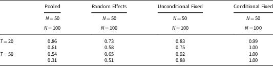
We report the results for four sets of experiments: 1) high endogeneity, low within variance (high-ρ, low-σ); 2) low endogeneity, low within variance (low-ρ, low-σ); 3) high endogeneity, high within variance (high-ρ, high-σ); and 4) low endogeneity, high within variance (low-ρ, high-σ). In the first set of experiments (Table 1), we set the within-unit variance σ to 1 (meaning the between-to-within, hereafter B/W, variation ratio is also 1) and the correlation between the predictor and the unit effect ρ to 0.50, varying the size of N (the number of units) and T (the number of time periods).Footnote ¹⁶ The high level of endogeneity should favor the fixed effects estimators in this case.

Table 1.

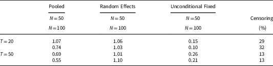
RMSE Ratios for PML-FE Coefficient Estimates (ρ=0.5, σ=1)

Note: RMSE ratios are relative to PML-FE results, such that values less than 1 indicate superior performance by PML-FE.

RMSE= root-mean squared error; PML-FE=penalized maximum likelihood fixed-effects.

The results in Table 1 show that the fixed effects models dominate the alternatives in root-mean squared error (RMSE) terms. More specifically, the numbers in the table are RMSE ratios that express the relative performance of PML-FE to the alternatives (listed in the table’s columns). Ratios less than 1 indicate the superiority of PML-FE. We see that the unconditional fixed effects estimator does consistently worse than the conditional fixed effects (and the PML-FE) estimator. Beck (Reference Beck2015) argues that the poor performance is attributable to the large number of parameters that are estimated in the unconditional fixed effects model. However, the PML-FE estimator, which the reader will recall is a modified estimation strategy for the unconditional fixed effects specification, does as well (and slightly better) than the conditional fixed effects model in recovering the coefficient estimates. The penalty-induced shrinkage in the PML-FE estimates seems to ameliorate the problem of proliferating parameters.Footnote ¹⁷

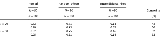
In all but the linear-additive model, coefficient estimates are not effect estimates. Most of the time we are interested in the (average) marginal effect of a predictor on the probability of observing the outcome, yet the conditional fixed effects estimator is unable to produce this estimate. This is one reason to prefer the random effects or unconditional fixed effects estimators to conditional fixed effects, despite the fact that the latter approach estimates the coefficient β relatively accurately. Our results (see Table 2) suggest that this might be a poor justification, as these estimators fail to accurately recover these effects.Footnote ¹⁸

Table 2.

RMSE Ratios for PML-FE Marginal Effects (ρ=0.5, σ=1)

Note: RMSE ratios are relative to PML-FE results, such that values less than 1 indicate superior performance by PML-FE. Censoring gives the percentage of units for which Y is never 1.

Beginning with unconditional fixed effects, the performance of the estimator relative to PML-FE is abysmal and depends on the number of censored units in the sample, which, in turn, depends on T. For T=20, the percentage of censored units is above 50 percent and the RMSE for PML-FE is about one-tenth the size as for the unconditional fixed effects estimator.Footnote ¹⁹ Since the censored units have systematically lower baseline probabilities of experiencing the event, the unconditional FE estimator produces a badly biased estimate of the AME. Additionally, the PML-FE AME estimates are superior to those produced by random effects. The endogeneity problem is compounded by the low within-unit variance in x _it to such an extent that that random effects is outperformed by PML-FE. Moreover, the size of this performance gap seems to be sensitive to N, with large N benefiting PML-FE relative to random effects. In sum, under these experimental conditions, the PML-FE estimator is able to recover coefficient estimates as accurate as conditional fixed effects and also produce the most accurate marginal effects estimates.

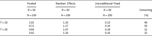
Decreasing the correlation between the predictor and the unit effect should reduce the MSE gains achieved from fixed effects, as random effects becomes less biased and more efficient. Therefore, in our second set of simulations, we reduce ρ to 0.25 holding all else constant. The results in Table 3 indicate that, as expected, random effects performs better and is now the preferred model. The RMSE of the sampling distribution for PML-FE estimator is between 27 percent and 47 percent larger than the RMSE for the random effects estimator, and the relative performance of random effects improves as N increases. Thus, when the overall level of endogeneity is high, increasing the number of units reduces the performance of the random effects estimator relative to PML-FE, but when the overall level of endogeneity is lowered, consistent with Beck’s proliferating parameters problem, the relative performance of random effects improves.

Table 3.

RMSE Ratios for PML-FE Marginal Effects (ρ=0.25, σ=1)

Note: RMSE ratios are relative to PML-FE results, such that values less than 1 indicate superior performance by PML-FE. Censoring gives the percentage of units for which Y is never 1.

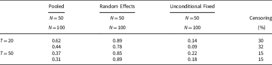
A second issue is the extent to which predictors change over time—that is, covariates for which the within variation are small relative to the between variation—as coefficients on slowly changing variables can be poorly estimated with fixed effects models (Plümper and Troeger Reference Plümper and Troeger2007). What happens when we increase the within unit variance for both the high and low endogeneity cases? For the experiment reported in Table 4, we increase the within-unit variance in the predictor for the high endogeneity case. This should benefit PML-FE by increasing the amount of information used to estimate the effects, but it also benefits the random effects estimator by reducing the overall degree of endogeneity in x _it . Comparing to Table 2, we see that the relative performance of random effects to PML-FE improves when we increase σ from 1 to 2. The implication of the findings in Tables 2 and 4 runs counter to the conventional wisdom. When the level of endogeneity is high, estimating the coefficients on predictors with little within-unit variation (e.g., slowly-changing predictors) using the fixed effects model actually does relatively better in comparison random effects.

Table 4.

RMSE Ratios for PML-FE Marginal Effects (ρ=0.5, σ=2)

Note: RMSE ratios are relative to PML-FE results, such that values less than 1 indicate superior performance by PML-FE. Censoring gives the percentage of units for which Y is never 1.

Comparing Tables 3 and 5, when the level of endogeneity is low (ρ=0.25), we see the opposite result: the relative performance of the PML-FE estimator improves. Overall, it is clear that the marginal benefits to the random effects and PML-FE estimators from increasing the within unit variance of the predictor depend on the strength of the correlation between x _i and α _i .Footnote ²⁰ When this correlation is strong, the improvements in the random effects estimator from reducing the endogeneity of the predictor (x _it ) are greater than the improvements in the penalized fixed effects estimator from increasing the amount of information available to estimate the coefficient β.

Table 5.

RMSE Ratios for PML-FE Marginal Effects (ρ=0.25, σ=2)

Note: RMSE ratios are relative to PML-FE results, such that values less than 1 indicate superior performance by PML-FE. Censoring gives the percentage of units for which Y is never 1.

In sum, our experiments suggest that the use of the pooled, unconditional, and conditional fixed effects estimators is rarely, if ever, justified with rare events data. With intercept heterogeneity, random effects typically outperforms the pooled estimator. If these unit effects are also correlated with the predictors, then PML-FE should often be preferred. In our simulations, PML-FE weakly dominated both unconditional and conditional fixed effects, providing coefficient estimates at least as good as the latter and more accurate marginal effects estimates than the former. The extent of these gains is both a function of the degree of censoring, as this biases the AME estimates from the unconditional fixed effects model.

The choice between random effects and PML-FE is less straight-forward and depends, not surprisingly, on the extent to which the orthogonality assumption of random effects is violated. As this is a theoretical choice that cannot be adjudicated empirically, there will always be a degree of subjectivity here. However, one bit of observable information that may be useful is the between-to-within variation in predictors. When one suspects a predictor is correlated with the unit effects, the lack of within-unit variation compounds this problem and weighs in favor of PML-FE rather than random effects. Generally, researchers should report both values and discuss what deviant results may tell us.

Illustration—the determinants of civil war

One of the research areas most prominently affected by the issues raised in the Dirty Pool symposium has been peace studies. This makes sense given the initial substantive focus of that discussion (i.e., the democratic peace) and the abundance of binary outcome models in this literature (e.g., conflict onset, alliance formation, regime transition, etc…). Despite this, a reading of this literature suggests that there remains little conceptual clarity on how best to model unobserved unit heterogeneity. Researchers frequently seem to confuse the issues underlying the decision over which modeling strategy to prefer. In particular, they seem skeptical of, and occasionally hostile toward, fixed effects estimation. Stemming from this confusion, researchers have largely failed to adopt a uniform approach for estimating unit effects.

The civil war literature, in particular, demonstrates this variation. Numerous papers make no attempt to model unit effects—preferring pooled logit or probit estimation—while those that do often adopt different approaches. For example, Fearon and Laitin (Reference Fearon and Laitin2003) re-estimate their main model(s) using conditional fixed effects logit and indicate that their results are “virtually identical” to the pooled estimates.Footnote ²¹ Instead, Sambanis (Reference Sambanis2001) re-estimates his models using random effects probit, ultimately preferring the simple probit estimator—despite rejecting the null of independence—because of the similarity in the results. Finally, Collier and Hoeffler (Reference Collier and Hoeffler2004) argue that fixed effects estimation is “very severe”—owing to sample censoring—yet they re-estimate their models with both random and fixed effects. Thus, even the canonical works in the civil war literature—with each of these articles having been cited more than 1000 times—disagree over the role of unobservables in the determination of civil war and how they should be addressed in empirical research.

This is troubling given that this issue is not simply one of taste or a methodological nuisance. Rather, it represents a significant theoretical belief, namely, whether we believe there are latent unobserved factors which cause some states to experience (avoid) civil conflict. More specifically, are there unobservables which may determine both conflict propensity and the included regressors? There are strong reasons to suspect this may be the case for some of the standard included determinants of civil war such as the level of development. In a different context, Acemoglu et al. (Reference Acemoglu, Johnson, Robinson and Yared2008) have challenged the effect of income on democratization, arguing that (unobserved and therefore unmodeled) historical factors influence both political and economic development. Similarly, in the case of civil war and development, some states have likely developed better conflict-management processes and resultant institutions. The ability to resolve low-level disputes without resorting to violence aided development and reduced the risk of future fighting. That is, to the extent that there is a relationship between development and fighting it is one borne out over hundreds of years. Conversely, those states which were unable to resolve such disputes peaceably were set back in their development—forced to devote resources to security, dispute resolution, fighting, etc.—and had a greater probability of future conflict.

If correct, this would mean that the relationship between the level of GDP and civil war is spurious, with both sharing a common cause. Pooled and random effects models do not offer insurance against this, risking bias due to these unobservables. Instead, researchers should prefer fixed effects estimation which partials out these potential unobserved (time-invariant) characteristics from the analysis. To examine these issues, we reanalyze Fearon and Laitin’s (Reference Fearon and Laitin2003) classic and oft-cited insurgency model which examines the determinants of civil war onset globally from 1945 to 1999. The dependent variable is binary, assuming a value of 1 for the first year of a civil war which is defined as conflict within a state in which both combatants (one representing the government) are politically organized and engage in fighting resulting 500 or more battle-related deaths and 0 otherwise. We also include a battery of standard regressors that include both time-varying (lagged war, logGDP, logPopulation, Polity, Oil, Instability, Non-Contig) and time-invariant measures (logMountain, Ethnic Fractionalization, Religious Fractionalization).Footnote ²²

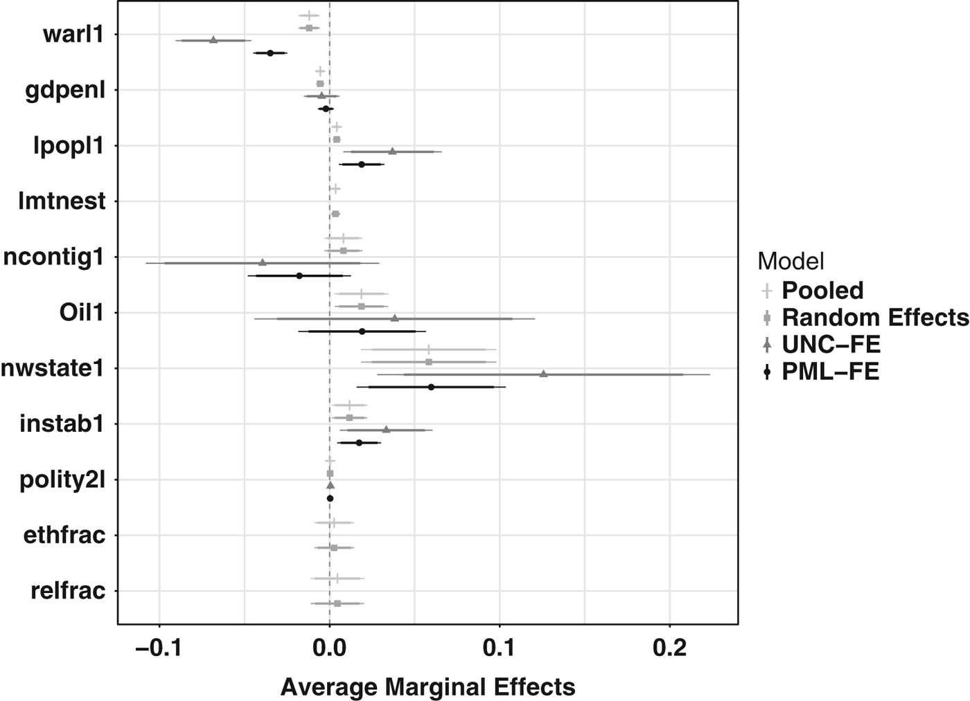
The results (presented in Figure 1) exhibit substantial differences between the various estimation strategies. There are notable differences between pooled/random effects and any of the fixed effects estimations.Footnote ²³ While some measures are robust to all specification—instability and population—others lose (gain) significance from the alternative approaches included, most notably, GDP per capita (gdpenl). As in Fearon and Laitin (Reference Fearon and Laitin2003), the pooled results suggest a negative and significant effect of GDP on civil war. The same is true when random intercepts are including, produces results that are effectively identical to those from the pooled model.Footnote ²⁴ The fixed effects models, however, suggest that the relationship between GDP and civil war is insignificant. This is substantial given that GDP is widely considered to be the most robust predictor of civil war onset (Hegre and Sambanis Reference Hegre and Sambanis2006). However, our results indicate that there is no within-unit effect of development on civil war, suggesting that these previous findings have been spurious.

Figure 1.

Unit heterogeneity in civil war onset (coefficients). Reanalysis of Fearon and Laitin (Reference Fearon and Laitin2003).

This finding in itself, is not novel—several researchers have observed and most dismissed it—what is more important is establishing that it is not a statistical artifact but instead a meaningful theory-driven result. While others have argued that these fixed effects results are biased—from “treating as non-informative all countries where we do not observe variation in the response,” (Buhaug and Gleditsch Reference Buhaug and Gleditsch2008, 227)—here we have shown that it is not due to sample censoring. Instead, the results suggest that there is no evidence that within-unit changes to development affect the probability of civil war onset.Footnote ²⁵

Next, we calculate the marginal effects of the determinants of civil war for each of the models (presented in Figure 2).Footnote ²⁶ Focusing on those predictors that are significant across all models, we observe quite different AMEs estimates (lpopl1, instab1, and warl1), with the fixed effects models suggesting larger effects. Comparing the unconditional fixed effects model and PML-FE, we see that unconditional fixed effects always returns a larger estimate. This is consistent with our expectation from Section 2 that because unconditional FE estimators will overestimate the baseline probability of conflict they will also overestimate the marginal effect of predictors. Here we see dramatic examples of that, as the effect of lagged war (warl) is nearly twice as large in the unconditional FE model (−0.068) as it is in the PML-FE model (−0.035). This is a dramatic shift given that the underlying specification of these two models is quite similar (i.e., the inclusion of unit dummies), with the only difference coming in how censored cases are treated in estimation.

Figure 2.

Unit heterogeneity in civil war onset (average marginal effects). Reanalysis of Fearon and Laitin (Reference Fearon and Laitin2003).