



1. Introduction
In numerous fluid dynamics problems, turbulence phenomena have garnered widespread attention due to their complexity and universality. Turbulent boundary layers (TBLs) over a flat plate and circular cylinder not only hold significant academic value but also play critical roles in the aviation, aerospace, marine engineering, automotive design and energy sectors (Bull Reference Bull1996). As a core physical quantity in flat-plate TBL research, the fluctuating wall pressure exhibits dual effects: direct radiation noise and excitation of structural vibration noise. Such spatio-temporally random distributed loads require characterisation through statistical analysis. Extensive research on TBL fluctuating pressure characteristics has been conducted via numerical simulations (Kim Reference Kim1989; Choi & Moin Reference Choi and Moin1990; Viazzo, Dejoan & Schiestel Reference Viazzo, Dejoan and Schiestel2001; Duan et al. Reference Duan, Choudhari and Wu2014, Reference Duan, Choudhari and Zhang2016; Gloerfelt & Berland Reference Gloerfelt and Berland2013; Panton, Lee & Moser Reference Panton, Lee and Moser2017; Zhang, Duan & Choudhari Reference Zhang, Duan and Choudhari2017; Ritos et al. Reference Ritos, Kokkinakis, Drikakis and Spottswood2017; Huang et al. Reference Huang, Duan, Casper, Wagnild and Bitter2024) and experimental methods (Schewe Reference Schewe1983; Farabee & Casarella Reference Farabee and Casarella1991; Keith, Hurdis & Abraham Reference Keith, Hurdis and Abraham1992; Beresh et al. Reference Beresh, Henfling, Spillers and Pruett2011; Cohen & Gloerfelt Reference Cohen and Gloerfelt2018; Zhao & Zhao Reference Zhao and Zhao2021). Spectral analysis of wall-pressure fluctuation time-domain signals yields correlation functions and power spectra (including auto-power spectra, cross-power spectra and wavenumber–frequency spectra). Based on these spectral characteristics, researchers have developed various predictive models for fluctuating wall-pressure wavenumber–frequency spectra, primarily categorised as theoretical models and empirical models.
Theoretical models are represented by those proposed by Chase (Chase Reference Chase1980, Reference Chase1987), Ffowcs Williams (Reference Williams1965), Burgeon Jr (Reference Bergeron and Robert1973), Dhanak (Reference Dhanak1988) and Doisy (Reference Doisy2017). Among these, the first four scholars focused on flat-plate models, while Dhanak investigated cylinder models. These models construct wavenumber–frequency spectra for TBL fluctuating wall pressure by introducing flat-plate/cylinder boundary conditions and relevant assumptions to solve either the acoustic wave equation or the momentum-continuity equations. Their primary strength lies in their clear physical mechanisms, facilitating parameter sensitivity analysis. However, they exhibit the following limitations: (i) no unified physical expression for fluctuating pressure across the entire wavenumber domain has been established: significant differences exist between the expression for fluctuating pressure in the convective region obtained via the Lighthill equation (see Ffowcs Williams (Reference Williams1965) and Dhanak (Reference Dhanak1988)) and the expression for fluctuating pressure in the acoustic region obtained via the momentum-continuity equations (Bergeron Jr Reference Bergeron and Robert1973). Current research literature still lacks a reasonable explanation for the above differences. Additionally, extrapolating the fluctuating pressure expressions applicable to specific wavenumber intervals to the entire wavenumber domain introduces significant prediction errors. (ii) Neglect of Mach number (
 ${\textit{Ma}}$
) effects: all derivations neglect the convective effect of incoming flow, failing to account for the Mach number’s role in the acoustic region of fluctuating pressure wavenumber–frequency spectra. (iii) Limitations in the cylinder model: Dhanak’s cylinder boundary layer study did not distinguish between the distances from image vortices and flow vortices to wall-receiving points.
Empirical models are represented by those developed by Corcos (Reference Corcos1963, Reference Corcos1964, Reference Corcos1967), Efimtsov (Reference Efimtsov1982) and Smol’yakov (Reference Smol’yakov2000, Reference Smol’Yakov2006). These models derive wavenumber–frequency spectra by introducing empirical expressions for the cross-spectral density of fluctuating wall pressure followed by spatio-temporal Fourier transforms. Their cross-spectral models decouple auto-spectral components, wavenumber components and attenuation components, significantly reducing modelling complexity. When combined with high-precision auto-spectral models (e.g. Goody Reference Goody2004), these models demonstrate excellent accuracy in predicting the amplitude of fluctuating pressure at the main energy concentration point (the ‘convective peak’). However, they suffer from fundamental limitations:
-
(i) lack of physical mechanisms: their purely data-driven nature neglects the influence mechanisms of turbulent eddies on fluctuating pressure.
-
(ii) Low-wavenumber region prediction inaccuracy: accuracy is only satisfactory in the convective peak region, with predictions deviating from reality at low wavenumbers and in the acoustic-frequency range.
-
(iii) Limitations in modifications: although Smol’yakov (Reference Smol’yakov2000, Reference Smol’Yakov2006) introduced mathematical corrections for the low-wavenumber/acoustic-frequency model, the absence of Mach number effects results in limited universality.
Research on fluctuating wall-pressure models has evolved over decades, yet the following common issues persist:
-
(i) Derived expressions for TBL fluctuating pressure exhibit discrepancies across different wavenumber ranges among scholars, with no unified formulation established.
-
(ii) Inadequate consideration of compressibility: medium (such as air, water, etc.) compressibility effects (particularly at Mach number 0.3) remain insufficiently addressed, limiting predictive capability for fluctuating pressure wavenumber–frequency spectra.
-
(iii) Low-wavenumber/acoustic-region discrepancies: significant deviations exist between predictions of existing models and experimental data in this region.
This study proposes targeted improvements:
-
(i) Establish a unified physical expression for fluctuating pressure across the entire wavenumber domain.
-
(ii) Develop a reconstructed compressible-flow pressure formulation that explicitly characterises Mach number effects in the acoustic region.
-
(iii) Integrate advantages from both theoretical and empirical models to construct novel wavenumber–frequency spectral models for fluctuating wall pressure in flat-plate and cylinder TBLs. The established model demonstrates enhanced prediction accuracy in both the low-wavenumber region and the acoustic region.
2. Model establishment
2.1. Fluctuating pressure-noise unified physical model
Before conducting research on the wavenumber–frequency spectrum of the fluctuating pressure in TBLs, we must recognise that wall fluctuating pressure energy primarily originates from flow eddies of varying scales and frequencies within the boundary layer. When these flow eddies are in close proximity to the wall’s reception point, we consider the wall’s fluctuating pressure to be predominantly influenced by the ‘pressure’ effect of the flow eddies. Conversely, when the flow eddies are distant from the wall’s reception point, we attribute the wall’s fluctuating pressure mainly to the ‘acoustic’ effect of the flow eddies. Although the ‘acoustic’ and ‘pressure’ effects appear to manifest distinctly based on the distance between the reception point and the source point, the precise relationship between them requires further elucidation in this paper.
This paper adopts the following assumptions:
-
(i) In the derivation of the formulas in this paper, all viscous effects are attributed to the velocity source term. The energy transfer process between the flow source and the wall pressure no longer considers viscous influences. The fundamental equations used are the continuity equation and the Euler equations.
-
(ii) The Goody model is employed in this study to determine the overall energy level of the fluctuating pressure wavenumber–frequency spectrum model, the applicability of the present model largely depends on that of the Goody model. Under extremely high Reynolds number conditions, the overall energy amplitude of the present model may exhibit certain deviations.
-
(iii) When deriving the fluctuating pressure in the TBL around a circular cylinder, it is assumed that the characteristic length of eddies within the cylinder boundary layer is significantly smaller than the cylinder’s radius, and that the flow structure within the cylinder boundary layer is identical to that in a flat-plate boundary layer. At very low frequencies – where the characteristic length of the eddies becomes large and no longer satisfies the assumption of being much smaller than the cylinder’s radius – the Goody model, which is based on flat-plate assumptions, may differ from the actual auto-spectrum of the fluctuating pressure in a cylindrical TBL. Consequently, at very low frequencies, the overall energy amplitude of the present model may also deviate to some extent.
2.1.1. Dimensional analysis
According to the fundamental theory of fluid mechanics, the flow velocity at low Mach numbers can be decomposed into the following form:
 \begin{equation} u_i = v_i+ \frac {\partial \psi }{\partial x_i}, \end{equation}
where
 $v_i$
is the induced velocity generated by the vortex in the flow;
 $\psi$
is the velocity potential;
 $x_i$
represents the coordinates of the receiving point in the streamwise, normal and spanwise directions.
The velocity potential
 $\psi$
can be determined by means of the continuity equation
 \begin{equation} {{\rho }^{-1}}\frac {\text{D}\rho }{\text{D}t}+{{\boldsymbol{\nabla} }^{2}}\psi =0\ , \end{equation}
where
 $\rho$
is the fluid density, and
 $t$
is the absolute time.
Further analysis of its dimensions reveals that
 \begin{equation} \frac {1}{\rho }\frac {\text{D}\rho }{\text{D}t}=\frac {1}{\rho c^2}\frac {\text{D}p}{\text{D}t}=O\left ( \frac {u}{\varLambda }{\textit{Ma}}^2 \right )\!, \end{equation}
where
 $c$
is the speed of sound in the medium,
 $p$
is the pressure,
 $u$
is the fluctuation velocity,
 $\varLambda$
is the characteristic scale of the flow and
 $t$
is the absolute time.
Thus (2.3) implies that
 \begin{align} \psi &=O\big ( \varLambda {{\textit{uMa}}^{2}} \big ), \end{align}
 \begin{align} \frac {\partial \psi }{\partial {{x}_{i}}}&=O\big ( {{\textit{uMa}}^{2}} \big ). \end{align}
Analysis shows that in low Mach number flows
 \begin{equation} u_i\approx v_i. \end{equation}
Under isentropic conditions, the following relationship holds:
 \begin{equation} {{\rho '}}={{{p'}}}/{{{c}^{2}}}\,=O\left ( {{\rho }_{0}}{{\textit{Ma}}^{2}} \right )\!, \end{equation}
where
 $\rho '$
and
 $p'$
denote the density and pressure fluctuations, respectively.
Through the above analysis, the variables are made dimensionless according to
 \begin{align} u,v&\sim U ,\end{align}
 \begin{align} {{\rho '}}&\sim {{\rho }_{0}}{\textit{Ma}}^2, \end{align}
 \begin{align} {{p'}}&\sim {{\rho }_{0}}{{u^2}},\\[-14pt]\nonumber \end{align}
 \begin{align} \frac {\partial \psi }{\partial {{x}_{i}}}&\sim u {\textit{Ma}}^2,\\[-14pt]\nonumber \end{align}
 \begin{align} {{x}_{i}}&\sim {\varLambda }/{\mu } , \end{align}
 \begin{align} t&\sim {\varLambda }/{U} , \end{align}
where
 $U$
is the average velocity of the flow and
 $\mu$
ranges from 1 to
 ${\textit{Ma}}$
, where
 $\mu = 1$
corresponds to the near field and
 $\mu = Ma$
corresponds to the far field.
2.1.2. Fluctuating pressure-noise theoretical model
Based on the above scaling relations, the dimensionless continuity and Euler equations for the near field can be expressed in the following form:
 \begin{align} {{\textit{Ma}}^{2}}\frac {\partial {\tilde {\rho }}'}{\partial \tilde {t}}+{{\textit{Ma}}^{2}}\left ( {{{\tilde {v}}}_{\!j}}+{{\textit{Ma}}^{2}}\frac {\partial \tilde {\psi }}{\partial {{{\tilde {x}}}_{\!j}}} \right )\frac {\partial {\tilde {\rho }}'}{\partial {{{\tilde {x}}}_{\!j}}}+{{\textit{Ma}}^{2}}\left ( 1+{{\textit{Ma}}^{2}}{\tilde {\rho }}' \right )\frac {{{\partial }^{2}}\tilde {\psi }}{\partial {{{\tilde {x}}}_{\!j}}^{2}}&=0, \end{align}
 \begin{align} \left ( 1+{{\textit{Ma}}^{2}}{{{\tilde {\rho }}'}} \right )\left [ \frac {\partial }{\partial \tilde {t}}\left ( {{{\tilde {v}}}_{i}}+{{\textit{Ma}}^{2}}\frac {\partial \tilde {\psi }}{\partial {{{\tilde {x}}}_{i}}} \right )+\left ( {{{\tilde {v}}}_{\!j}}+{{\textit{Ma}}^{2}}\frac {\partial \tilde {\psi }}{\partial {{{\tilde {x}}}_{\!j}}} \right )\frac {\partial }{\partial {{{\tilde {x}}}_{\!j}}}\left ( {{{\tilde {v}}}_{i}}+{{\textit{Ma}}^{2}}\frac {\partial \tilde {\psi }}{\partial {{{\tilde {x}}}_{i}}} \right ) \right ]&=-\frac {\partial {{\tilde {p}'}}}{\partial {{{\tilde {x}}}_{i}}}. \end{align}
Continuing the mathematical transformation of the above two expressions yields
 \begin{align} {\textit{Ma}}^{2}\frac {{{\partial }^{2}}{{\tilde {\rho }'}}}{\partial {{\tilde {t}}^{2}}}-\frac {{{\partial }^{2}}{{\tilde {\rho }'}}}{\partial \tilde {x}_{\!j}^{2}}&=\frac {{{\partial }^{2}}{{\tilde {T}}_{\textit{ij}}}}{\partial {{\tilde {x}}_{i}}\partial {{\tilde {x}}_{\!j}}},\end{align}
 \begin{align} {{\tilde {T}}_{\textit{ij}}}&=\big ( 1+{{\textit{Ma}}^{2}}{{\tilde {\rho }'}} \big )\big ( \tilde {{{v}_{i}}}+{{\textit{Ma}}^{2}}\tilde {{{\psi }_{i}}} \big )\big ( \tilde {{{v}_{\!j}}}+{{\textit{Ma}}^{2}}\tilde {{{\psi }_{\!j}}} \big )+\left ( {{\tilde {p}'}}-{{\tilde {\rho }'}} \right )\!,\end{align}
 \begin{align} {{\tilde {p}'}}-{{\tilde {\rho }'}}&=O\big ( {{\textit{Ma}}^{2}} \big ),\end{align}
where
 $\overset {\tilde {\ }}{\mathop {{}}}\,$
denotes an averaging operation,
 $\tilde {\psi }_i=({\partial \tilde {\psi }}/{\partial \tilde {x}_i})$
.
Given that our study focuses on fluctuating pressure and noise phenomena in low Mach number flows, the influence of higher-order Mach number terms (second order and above) on the final results is negligible (Lighthill Reference Lighthill1952, Reference Lighthill1954). By retaining only the leading-order terms and neglecting all higher-order Mach number contributions, the following relationship can be derived from (2.16) and (2.17):
 \begin{align} -\frac {{{\partial }^{2}}{{\tilde {p}'}}}{\partial \tilde {x}_{\!j}^{2}}&=\frac {{{\partial }^{2}}{{\tilde {T}}_{\textit{ij}}}}{\partial {{\tilde {x}}_{i}}\partial {{\tilde {x}}_{\!j}}}, \end{align}
 \begin{align} {{\tilde {T}}_{\textit{ij}}}&=\tilde {{{v}_{i}}}\tilde {{{v}_{\!j}}}. \end{align}
The solution for near-field fluctuating pressure is
 \begin{equation} \tilde {p}'=\frac {1}{4\pi }\int {\frac {1}{\tilde {r}}}\frac {\partial ^2\left ( \tilde {v}_i\tilde {v}_j \right )}{\partial \tilde {y}_i\partial \tilde {y}_j}\,\text{d}\,\tilde {y}_1\,\text{d}\tilde {y}_2\,\text{d}\tilde {y}_3, \end{equation}
where
 $r$
is the distance between the receiving point and the source point;
 $y_1, y_2, y_3$
are the coordinates of source point in streamwise, normal and spanwise directions.
Correspondingly, for the far-field scenario, applying mathematical transformations to the dimensionless continuity and Euler equations yields the following relationship:
 \begin{align} \frac {\partial ^2\tilde {\rho }'}{\partial \tilde {t}^2}-\frac {\partial ^2\tilde {\rho }'}{\partial \tilde {x}_{\!j}^{2}}&=\frac {\partial ^2\tilde {T}_{\textit{ij}}}{\partial \tilde {x}_i\partial \tilde {x}_i},\end{align}
 \begin{align} {{\tilde {T}}_{\textit{ij}}}&=\left ( 1+{{\textit{Ma}}^{2}}{{\tilde {\rho }'}} \right )\left ( \tilde {{{v}_{i}}}+{{\textit{Ma}}^{3}}\tilde {{{\psi }_{i}}} \right )\left ( \tilde {{{v}_{\!j}}}+{{\textit{Ma}}^{3}}\tilde {{{\psi }_{\!j}}} \right )+\left ( {{\tilde {p}'}}-{{\tilde {\rho }'}} \right )\!.\end{align}
By neglecting all higher-order Mach number terms, the following relationship can be derived from (2.22) and (2.23):
 \begin{align} \frac {{{\partial }^{2}}{{\tilde {p}'}}}{\partial {{\tilde {t}}^{2}}}-\frac {{{\partial }^{2}}{{\tilde {p}'}}}{\partial \tilde {x}_{\!j}^{2}}&=\frac {{{\partial }^{2}}{{\tilde {T}}_{\textit{ij}}}}{\partial {{\tilde {x}}_{i}}\partial {{\tilde {x}}_{\!j}}},\end{align}
 \begin{align} {{\tilde {T}}_{\textit{ij}}}&=\tilde {{{v}_{i}}}\tilde {{{v}_{\!j}}}.\end{align}
The solution for far-field noise is
 \begin{equation} \tilde {p}'=\frac {1}{4\pi }\int {\frac {1}{\tilde {r}}\left [ \frac {\partial ^2\tilde {v}_i\tilde {v}_j}{\partial \tilde {y}_i\partial \tilde {y}_j} \right ] _{\tilde {\tau }=\tilde {t}-\tilde {r}}}\text{d}\tilde {y}_1\text{d}\tilde {y}_2\text{d}\tilde {y}_3, \end{equation}
where
 $\tau$
is the retarded time.
Observation reveals that the source terms for the near-field and far-field fluctuating pressures (representing the dominant energy components) are identical. However, the governing equations evolve from the Laplace equation to the wave equation. We will now analyse the intermediate-field fluctuating pressure between these regimes.
For the intermediate field, applying mathematical transformations to the dimensionless continuity and Euler equations yields the following relationship:
 \begin{align} {{\left ( \frac {\textit{Ma}}{\mu } \right )}^{2}}\frac {{{\partial }^{2}}{{\tilde {\rho }'}}}{\partial {{\tilde {t}}^{2}}}-\frac {{{\partial }^{2}}{{\tilde {\rho }'}}}{\partial \tilde {x}_{\!j}^{2}}&=\frac {{{\partial }^{2}}{{\tilde {T}}_{\textit{ij}}}}{\partial {{\tilde {x}}_{i}}\partial {{\tilde {x}}_{\!j}}},\end{align}
 \begin{align} {{\tilde {T}}_{\textit{ij}}}&=\left ( 1+{\textit{Ma}}^2 {{\tilde {\rho }'}} \right )\left ( \tilde {{{v}}}_{i}+\mu {\textit{Ma}}^2\tilde {{{\psi }}}_{i} \right )\left ( \tilde {{v}}_{\!j}+\mu {\textit{Ma}}^2 \tilde {{{\psi }}}_{\!j} \right )+\left ( {{\tilde {p}'}}-{{\tilde {\rho }'}} \right )\!.\end{align}
Observing (2.27), if the term
 ${\tilde {T}}_{\textit{ij}}$
on the right-hand side were independent of
 ${\tilde {\rho }'}$
, the equation would reduce to a standard wave equation. However, since
 ${\tilde {T}}_{\textit{ij}}$
actually depends on
 ${\tilde {\rho }'}$
, exact analytical solution is intractable. Analysis reveals that the left-hand side of the equation governs the phase relationship, while the right-hand side (source term) determines the amplitude magnitude. Although higher-order terms negligibly affect the amplitude magnitude, they may significantly influence phase relationships. Consequently, such terms cannot be neglected on the left-hand side but are negligible within the source term. Careful examination reveals that, within the source term, despite
 ${\tilde {T}}_{\textit{ij}}$
dependence on
 ${\tilde {\rho }'}$
, the scaling relations
 ${{\tilde {\rho }'}}\sim 1$
,
 $\tilde {{{\psi }}}_{i}\sim 1$
and
 $ ( {{\tilde {p}'}}-{{\tilde {\rho }'}} )\sim {{\textit{Ma}}^{2}}$
hold. Neglecting higher-order
 ${\textit{Ma}}$
terms (which are indeed negligible compared with leading-order quantities) yields
 ${{\tilde {T}}_{\textit{ij}}}\approx \tilde {{{v}}}_{i}\tilde {{{v}}}_{\!j}$
. Under this assumption, solving the differential equation becomes straightforward. We now proceed to directly solve the equation
 \begin{align} {{\left ( \frac {\textit{Ma}}{\mu } \right )}^{2}}\frac {{{\partial }^{2}}{{\tilde {\rho }'}}}{\partial {{\tilde {t}}^{2}}}-\frac {{{\partial }^{2}}{{\tilde {\rho }'}}}{\partial \tilde {x}_{\!j}^{2}}&=\frac {{{\partial }^{2}}\left ( \tilde {{{v}}}_{i}\tilde {{{v}}}_{\!j} \right )}{\partial {{\tilde {x}}_{i}}\partial {{\tilde {x}}_{\!j}}}, \end{align}
 \begin{align} \frac {{{\partial }^{2}}{{\tilde {\rho }'}}}{\partial {{\tilde {t}}^{2}}}-{{\left ( \frac {\mu }{\textit{Ma}} \right )}^{2}}\frac {{{\partial }^{2}}{{\tilde {\rho }'}}}{\partial \tilde {x}_{\!j}^{2}}&={{\left ( \frac {\mu }{\textit{Ma}} \right )}^{2}}\frac {{{\partial }^{2}}\left ( \tilde {{{v}}}_{i}\tilde {{{v}}}_{\!j} \right )}{\partial {{\tilde {x}}_{i}}\partial {{\tilde {x}}_{\!j}}}. \end{align}
The solution for intermediate-field fluctuating pressure/noise is
 \begin{align} {{\tilde {p}'}}={{\tilde {\rho }'}}&=\frac {1}{4\pi {{\left ( \frac {\mu }{\textit{Ma}} \right )}^{2}}}{{\left ( \frac {\mu }{\textit{Ma}} \right )}^{2}}\frac {{{\partial }^{2}}}{\partial {{\tilde {x}}_{i}}\partial {{\tilde {x}}_{\!j}}}\int {\frac {{{\left [ \tilde {{{v}}}_{i}\tilde {{{v}}}_{\!j} \right ]}_{\tilde {\tau }=\tilde {t}-\tilde {r}\Big ( \tfrac {\textit{Ma}}{\mu } \Big )}}}{\tilde {r}}}\text{d}\tilde {{{y}_{1}}}\text{d}\tilde {{{y}_{2}}}\text{d}\tilde {{{y}_{3}}}, \end{align}
 \begin{align} \tilde {p}'&=\frac {1}{4\pi }\int {\frac {1}{\tilde {r}}\left [ \frac {\partial ^2\tilde {v}_i\tilde {v}_j}{\partial \tilde {y}_i\partial \tilde {y}_j} \right ] _{\tilde {\tau }=\tilde {t}-\tilde {r}\Big ( \tfrac {\textit{Ma}}{\mu } \Big )}}\text{d}\tilde {y}_1\text{d}\tilde {y}_2\text{d}\tilde {y}_3. \end{align}
It can be seen that the only difference among near-field, intermediate-field and far-field fluctuating pressure/noise lies in the retardation time, that is, the time required for flow sources to propagate to the reception point. When
 $\mu ={\textit{Ma}}$
, this solution completely coincides with the far-field solution; when
 $\mu =\text{1}$
, since
 $\tilde {r}\sim O ( 1 )$
,
 $\tilde {\tau }=\tilde {t}-\tilde {r}Ma\approx \tilde {t}$
, meaning the propagation time from source to receiver is negligible. At this point, the solution also completely matches the near-field solution. These results demonstrate that fluctuating pressure and noise share a unified mathematical form.
All derivations above are based on the fundamental assumption of neglecting higher-order
 ${\textit{Ma}}$
terms (second order and above) in the source terms. Therefore, the derived theoretical model is applicable for predicting the fluctuating pressure auto-spectrum, correlations and root mean square values. However, whether these derivation results apply to the wavenumber–frequency spectrum of the fluctuating pressure (especially in low-energy acoustic regions and low-wavenumber zones) remains questionable. Next, we will focus on studying the theoretical model for the wavenumber–frequency spectrum of fluctuating pressure.
2.2. Derivation of the turbulent boundary layer fluctuating pressure wavenumber–frequency spectrum model considering Mach number effects
2.2.1. Governing equations and their solutions for fluctuating pressure in turbulent boundary layer
Here, we still commence from the dimensionless (2.14) and (2.15). After invoking the isentropic assumption, (2.14) and (2.15) can be simplified to the following form:
 \begin{align} \frac {\partial {{\tilde {u}}_{\!j}}}{\partial {{{\tilde {x}}}_{\!j}}}&=-{{\textit{Ma}}^{2}}\left [ \frac {\partial {{\tilde {p}'}}}{\partial \tilde {t}}+{{\tilde {u}}_{\!j}}\frac {\partial {{\tilde {p}'}}}{\partial {{{\tilde {x}}}_{\!j}}} \right ]\!,\end{align}
 \begin{align} \left ( 1+{{\textit{Ma}}^{2}}{{\tilde {p}'}} \right )\left [ \frac {\partial }{\partial \tilde {t}}{{\tilde {u}}_{i}}+{{\tilde {u}}_{\!j}}\frac {\partial }{\partial {{{\tilde {x}}}_{\!j}}}{{\tilde {u}}_{i}} \right ]&=-\frac {\partial {{\tilde {p}'}}}{\partial {{{\tilde {x}}}_{i}}}.\end{align}
Here, the velocity is decomposed into mean velocity and fluctuating velocity
 \begin{equation} {{\tilde {u}}_{i}}=U\left ({{\tilde {x}}}_{2} \right )+{{\tilde {u}}_{i}^{\prime}}. \end{equation}
Substituting the above expressions into (2.33) and (2.34), neglecting all mean quantities and simplifying, yields
 \begin{align} L\left ( {{\tilde {u}}_{i}^{\prime}} \right )+{{\tilde {u}}_{\!j}}\frac {\partial }{\partial {{{\tilde {x}}}_{\!j}}}U\left ( {{{\tilde {x}}}_{2}} \right )+\frac {\partial {{\tilde {p}'}}}{\partial {{{\tilde {x}}}_{i}}}+{{\tilde {T}}_{i}}+{{\textit{Ma}}^{2}}\tilde {{{S}_{i}}}&=0,\end{align}
 \begin{align} \frac {\partial {{\tilde {u}}_{\!j}^{\prime}}}{\partial {{{\tilde {x}}}_{\!j}}}&=-{{\textit{Ma}}^{2}}\left [ L\left ( {{\tilde {p}'}} \right )+{{\tilde {u}}_{\!j}^{\prime}}\frac {\partial {{\tilde {p}'}}}{\partial {{{\tilde {x}}}_{\!j}}} \right ]\!,\end{align}
where
 \begin{align} L&=\frac {\partial }{\partial \tilde {t}}+U\left ( {{\tilde {x}}}_{2} \right )\frac {\partial }{\partial {{{\tilde {x}}}_{1}}}, \end{align}
 \begin{align} {{\tilde {T}}_{i}}&=\frac {\partial \left ( {{\tilde {T}}_{\textit{ij}}} \right )}{\partial {{{\tilde {x}}}_{\!j}}}, \end{align}
 \begin{align} {{\tilde {T}}_{\textit{ij}}}&={{\tilde {u}}_{i}^{\prime}}{{\tilde {u}}_{\!j}^{\prime}}, \end{align}
 \begin{align} \tilde {S}_i&=\tilde {u}_i'\left [ L\left ( \tilde {p}' \right ) +\tilde {u}_j\frac {\partial \tilde {p}'}{\partial \tilde {x}_j} \right ] -\frac {1}{2}\frac {\partial \left ( \tilde {p}'^2 \right )}{\partial \tilde {x}_i}. \end{align}
Performing mathematical transformations on (2.36) and (2.37) yields the following:
 \begin{equation} \frac {{{\partial }^{2}}{{\tilde {p}'}}}{\partial {{{\tilde {x}}}_{\!j}}^{2}}+2\frac {\partial U\left ( {{{\tilde {x}}}_{2}} \right )}{\partial {{{\tilde {x}}}_{2}}}\frac {\partial {{\tilde {u}}_{2}}}{\partial {{{\tilde {x}}}_{1}}}+\frac {\partial {{\tilde {T}}_{\!j}}}{\partial {{{\tilde {x}}}_{\!j}}}+{{\textit{Ma}}^{2}}\left \{ \frac {\partial \tilde {{{S}_{i}}}}{\partial {{{\tilde {x}}}_{\!j}}}-L\left [ L\left ( {{\tilde {p}'}} \right )+\frac {\partial }{\partial {{{\tilde {x}}}_{\!j}}}\left ( {{\tilde {p}'}}{{\tilde {u}}_{\!j}} \right ) \right ] \right \}=0 .\end{equation}
Applying the Fourier transform in time and space to (2.42) yields
 \begin{align} \left ( \textrm{D}^2 - k^2 \right ) \hat {p} + {\textit{Ma}}^2 \left ( \omega - k_1 U \right )^2 \hat {p} &= 2i k_1 D U \hat {u}_2 - \left [ \textrm{D}^2 \hat {T}_{22} - 2i \left ( k_1 \hat {T}_{12} + k_3 \hat {T}_{32} \right ) \right ] \notag\\ &\quad + \left ( k_1^2 \hat {T}_{11} + 2 k_1 k_3 \hat {T}_{13} + k_3^2 \hat {T}_{33} \right ) \notag\\ &\quad - {\textit{Ma}}^2 \left [ D \hat {\varGamma }_2 - i \left ( k_1 \hat {\varGamma }_1 + k_3 \hat {\varGamma }_3 \right ) \right ]\!,\end{align}
 \begin{align} {{\hat {\varGamma }}_{i}}&={{\hat {S}}_{i}}+i\left ( \omega -{{k}_{1}}U \right )\left ( {{{\hat {p}}'}}{{{\hat {u}}}_{i}} \right )\!,\end{align}
 \begin{align} {{k}^{2}}&={{k}_{1}}^{2}+{{k}_{3}}^{2},\end{align}
where
 $\omega$
is the angular frequency;
 $k_1$
,
 $k_2$
and
 $k_3$
are the wavenumbers in the streamwise, wall-normal and spanwise directions, respectively,
 $D={\text{d}}/{\text{d}{\tilde {x}_{2}}}$
is the differential operator and the hat symbol (
 $\hat {\phantom {\boldsymbol{\cdot }}}$
) denotes the Fourier transform. Given that
 $\omega =O ( 1 )$
, the appropriate wavenumber scaling across the entire wavenumber range should take the following form:
 \begin{align} {{k}_{1}}&=\mu \alpha ,\end{align}
 \begin{align} {{k}_{3}}&=\mu \beta ,\end{align}
 \begin{align} k&=\mu \gamma ,\end{align}
where
 $\mu$
ranges between 1 and
 ${\textit{Ma}}$
, reflecting the transition from the convective region to the acoustic region. When the wavenumber is at the convective peak,
 ${{k}_{1}}=\alpha$
; when in the acoustic region,
 ${{k}_{1}}={\textit{Ma}}\alpha$
.
Substituting these dimensional relationships into (2.43) yields
 \begin{equation} \begin{aligned} \textrm{D}^2 \hat {p} - \left [ \mu ^2 \gamma ^2 - {\textit{Ma}}^2 (\omega -\mu \alpha U) ^2 \right ] \hat {p} &= 2i \mu \alpha D U \hat {u}_2 \\ &\quad - \left [ \textrm{D}^2 \hat {T}_{22} - 2i \mu \left ( \alpha D \hat {T}_{12} + \beta D \hat {T}_{32} \right ) \right ] \\ &\quad + \mu ^2 \left ( \alpha ^2 \hat {T}_{11} + 2\alpha \beta \hat {T}_{13} + \beta ^2 \hat {T}_{33} \right ) \\ &\quad - {\textit{Ma}}^2 \left [ D \hat {\varGamma }_2 - i \mu \left ( \alpha \hat {\varGamma }_1 + \beta \hat {\varGamma }_3 \right ) \right ]\!. \end{aligned} \end{equation}
It is noted that the above equation can be simplified to the form
 ${{y''}}-{{a}^{2}}y=f ( x )$
. We now proceed to solve this equation.
The boundary conditions can be written as: when
 $x = 0$
,
 $f ( x )={{y'}} ( 0 )=0$
(Neumann condition); when
 $y \to \infty$
,
 $f ( x )=y=0$
.
The Green’s function
 $G ( x,\zeta )$
is defined to satisfy the following relationship:
 \begin{equation} {{G''}}-{{a}^{2}}G=\delta \left ( x-\zeta \right )\!,\begin{matrix} {} & {} \\ \end{matrix}x,\zeta \gt 0, \end{equation}
where
 $\delta$
is the Dirac function. The boundary conditions of Green’s function can be written as: when
 $x = 0$
,
 ${{\left . {\partial G}/{\partial x}\, \right |}_{x=0}}=0$
; when
 $x \to \infty$
,
 $G ( x,\zeta )=0$
.
The solution for the Green’s function can be expressed as
 \begin{equation} G\left ( x,\zeta \right )=\left \{\!\! \begin{array}{ll} -\dfrac {1}{a}{{e}^{-a\zeta }}\cosh \left ( ax \right )\!,&0\le x\le \zeta ,\\[8pt] -\dfrac {1}{a}\cosh \left ( a\zeta \right ){{e}^{-ax}},&0\le \zeta \le x. \\ \end{array} \right . \end{equation}
The solution for
 $y$
at this stage can be expressed as
 \begin{equation} y\left ( x \right )=\int _{0}^{\infty }{G\left ( x,\zeta \right )f\left ( \zeta \right )\text{d}\zeta }. \end{equation}
When
 $x = 0$
,
 $y ( 0 )$
can be expressed as
 \begin{equation} y\left ( 0 \right )=\int _{0}^{\infty }{G\left ( 0,\zeta \right )f\left ( \zeta \right )\text{d}\zeta }=-\frac {1}{a}\int _{0}^{\infty }{f\left ( \zeta \right ){{e}^{-a\zeta }}\text{d}\zeta }. \end{equation}
Returning to (2.49), the solution for this equation can be expressed as
 \begin{align} \hat {p} &= \frac {1}{\sqrt {\mu ^{2}\gamma ^{2} - {\textit{Ma}}^{2} (\omega -\mu \alpha U) ^2}} \notag\\ &\quad \times \int _{0}^{\infty } \left \{ \begin{aligned} & 2i\mu \alpha DU\hat {u}_{2} - \left [ D^{2}\hat {T}_{22} - 2i\mu \left ( \alpha \textrm{D}\hat {T}_{12} + \beta \textrm{D}\hat {T}_{32} \right ) \right ] \notag\\ & + \mu ^{2} \left ( \alpha ^{2}\hat {T}_{11} + 2\alpha \beta \hat {T}_{13} + \beta ^{2}\hat {T}_{33} \right ) \\ & - {\textit{Ma}}^{2} \left [ \textrm{D}\hat {\varGamma }_{2} - i\mu \left ( \alpha \hat {\varGamma }_{1} + \beta \hat {\varGamma }_{3} \right ) \right ] \\ \end{aligned} \right \} \notag\\ &\quad \times e^{-\sqrt {\mu ^{2}\gamma ^{2} - {\textit{Ma}}^{2} (\omega -\mu \alpha U) ^2} x_{2}} \, \text{d} x_{2} \notag\\ &= \frac {1}{\sqrt {\gamma ^{2} - (Ma/\mu )^{2} (\omega -\mu \alpha U) ^2}} \notag\\ &\quad \times \int _{0}^{\infty } \left \{ \begin{aligned} & 2i\alpha DU\hat {u}_{2} - \mu \left [ \gamma ^{2} - (Ma/\mu )^{2} (\omega -\mu \alpha U) ^2 \right ] \hat {T}_{22} \notag\\ & + 2i\mu \sqrt {\gamma ^{2} - (Ma/\mu )^{2} (\omega -\mu \alpha U) ^2} \left ( \alpha \hat {T}_{12} + \beta \hat {T}_{32} \right ) \notag\\ & + \mu \left ( \alpha ^{2}\hat {T}_{11} + 2\alpha \beta \hat {T}_{13} + \beta ^{2}\hat {T}_{33} \right ) \notag \\ & - {\textit{Ma}}^{2} \left [ \sqrt {\gamma ^{2} - (Ma/\mu )^{2} (\omega -\mu \alpha U) ^2} \, \hat {\varGamma }_{2} - i \left ( \alpha \hat {\varGamma }_{1} + \beta \hat {\varGamma }_{3} \right ) \right ] \\ \end{aligned} \right \} \notag\\ &\quad \times e^{-\sqrt {\mu ^{2}\gamma ^{2} - {\textit{Ma}}^{2}(\omega -\mu \alpha U) ^2} x_{2}} \,\text{d} x_{2}. \end{align}
Observing the above expression reveals that the expression for
 $p'$
simultaneously contains zeroth-order, first-order (when
 $\mu ={\textit{Ma}}$
) and higher-order (second order and above)
 ${\textit{Ma}}$
terms. Therefore, higher-order
 ${\textit{Ma}}$
terms can be directly neglected here, and the final expression for
 $p$
simplifies to
 \begin{align} \hat {p} &= \frac {1}{\sqrt {\gamma ^2 - \left ( \frac {\textit{Ma}}{\mu } \right )^2 (\omega -\mu \alpha U) ^2}} \notag\\ & \quad \times \int _{0}^{\infty } \left \{ \begin{aligned} & 2i\alpha \textit{DU} \hat {u}_2 - \mu \left [ \gamma ^2 - \left ( \frac {\textit{Ma}}{\mu } \right )^2 (\omega -\mu \alpha U) ^2 \right ] \hat {T}_{22} \notag\\ & + 2i\mu \sqrt {\gamma ^2 - \left ( \frac {\textit{Ma}}{\mu } \right )^2 (\omega -\mu \alpha U) ^2} \left ( \alpha \hat {T}_{12} + \beta \hat {T}_{32} \right ) \notag\\ & + \mu \left ( \alpha ^2 \hat {T}_{11} + 2\alpha \beta \hat {T}_{13} + \beta ^2 \hat {T}_{33} \right ) \end{aligned} \right \} \notag\\ &\quad \times e^{-\sqrt {\mu ^2 \gamma ^2 - {\textit{Ma}}^2 (\omega -\mu \alpha U) ^2} x_2} \text{d}x_2. \end{align}
Observation shows that, when
 $\mu =1$
, (2.55) can be written as
 \begin{align} \hat {p} &= \frac {1}{\sqrt {k^2 - {\textit{Ma}}^2 (\omega -k_1 U) ^2}} \notag\\ & \quad \times \int _{0}^{\infty } \left \{ \begin{aligned} & 2i k_1 D U \hat {u}_2 - (k^2 - {\textit{Ma}}^2 (\omega -k_1 U) ^2) \hat {T}_{22} \notag\\ & + 2i \sqrt {k^2 - {\textit{Ma}}^2 (\omega -k_1 U)^2} \left ( k_1 \hat {T}_{12} + k_3 \hat {T}_{32} \right ) \notag\\ & + \left ( k_1^2 \hat {T}_{11} + 2k_1 k_3 \hat {T}_{13} + k_3^2 \hat {T}_{33} \right ) \end{aligned} \right \} \notag\\ &\quad \times e^{-\sqrt {k^2 - {\textit{Ma}}^2 (\omega -k_1 U)^2} x_2} \text{d}x_2. \end{align}
The above equation represents the expression for the convective region
 $k^2\gg {\textit{Ma}}^2 ( \omega -k_1U ) ^2$
of the fluctuating pressure. After dimensionalisation, this form is entirely consistent with the expression derived by Ffowcs Williams (Reference Williams1965).
When
 $\mu ={\textit{Ma}}$
, the above expression can be written as
 \begin{align} \hat {p} &= \frac {1}{\sqrt {\gamma ^2 - (\omega -{\textit{Ma}} \alpha U) ^2}} \notag\\ &\quad \times \int _{0}^{\infty } \left \{ \begin{aligned} &2i\alpha\kern-1pt \textit{DU}\kern-1pt \hat {u}_2 - \textit{Ma}\left [ \gamma ^2 - (\omega -{\textit{Ma}} \alpha U) ^2 \right ] \hat {T}_{22} \notag\\ &+ 2\textit{iMa}\sqrt {\gamma ^2 - (\omega -{\textit{Ma}} \alpha U) ^2} \big ( \alpha \hat {T}_{12} + \beta \hat {T}_{32} \big ) \notag\\ &+ Ma\left ( \alpha ^2 \hat {T}_{11} + 2\alpha \beta \hat {T}_{13} + \beta ^2 \hat {T}_{33} \right ) \end{aligned} \right \} \notag\\ &\quad \times e^{-{\textit{Ma}}\sqrt {\gamma ^2 - (\omega -{\textit{Ma}} \alpha U) ^2} x_2} \text{d}x_2. \end{align}
Applying specific mathematical transformations to the
 ${\hat {u}}_{2}$
term in the above expression, it can be deduced from (2.36) that
 \begin{equation} \frac {\partial \tilde {u}_2}{\partial \tilde {t}} + U\frac {\partial \tilde {u}_2}{\partial \tilde {x}_1} + \frac {\partial \tilde {p}}{\partial \tilde {x}_2} + \frac {\partial \tilde {T}_{12}}{\partial \tilde {x}_1} + \frac {\partial \tilde {T}_{22}}{\partial \tilde {x}_2} + \frac {\partial \tilde {T}_{32}}{\partial \tilde {x}_3} + {\textit{Ma}}^2 \tilde {S}_2 = 0. \end{equation}
Applying the Fourier transform in space and time to the above equation yields
 \begin{equation} i\omega \hat {u}_2 - iU k_1 \hat {u}_2 + \textrm{D}\hat {p} - i k_1 \hat {T}_{12} + \textrm{D}\hat {T}_{22} - i k_3 \hat {T}_{32} + {\textit{Ma}}^2 \hat {S}_2 = 0. \end{equation}
Applying a scaling transformation in wavenumber to the above expression
 \begin{align} {{k}_{1}}&={\textit{Ma}}\alpha , \end{align}
 \begin{align} {{k}_{3}}&={\textit{Ma}}\beta , \end{align}
 \begin{align} k&={\textit{Ma}}\gamma . \end{align}
At this stage, (2.36) can be expressed as

Therefore, the expression for
 $\hat {u}_2$
can be written as follows:
 \begin{equation} {{\hat {u}}_{2}}=\frac {1}{i\omega }\left [ -{\rm D}\hat {p}-{\rm D}{{{\hat {T}}}_{22}}+\textit{iMa}\left ( U\alpha {{{\hat {u}}}_{2}}+\alpha {{{\hat {T}}}_{12}}+\beta {{{\hat {T}}}_{32}} \right )-{{\textit{Ma}}^{2}}{{{\hat {S}}}_{2}} \right ]\!. \end{equation}
Here, it is necessary to further establish the fundamental relationship between
 $\text{D}p$
and
 $D{{T}_{22}}$
. According to (2.49), the governing equation for fluctuating pressure can be derived as follows when
 $\mu ={\textit{Ma}}$
:
 \begin{equation} \begin{aligned} \textrm{D}^2 \hat {p} - {\textit{Ma}}^2 \left ( \gamma ^2 - (\omega -{\textit{Ma}} \alpha U) ^2 \right ) \hat {p} &= 2\textit{iMa}\alpha \textit{DU} \hat {u}_2 \\ &\quad - \left [ \textrm{D}^2 \hat {T}_{22} - 2\textit{iMa} \left ( \alpha D \hat {T}_{12} + \beta D \hat {T}_{32} \right ) \right ] \\ &\quad + {\textit{Ma}}^2 \left ( \alpha ^2 \hat {T}_{11} + 2\alpha \beta \hat {T}_{13} + \beta ^2 \hat {T}_{33} \right ) \\ &\quad - {\textit{Ma}}^2 \left [ D \hat {\varGamma }_{2} - \textit{iMa} \left ( \alpha \hat {\varGamma }_{1} + \beta \hat {\varGamma }_{3} \right ) \right ]\!. \end{aligned} \end{equation}
Here, the fundamental idea of the perturbation method is adopted. Assuming that
 $\hat {p} = \hat {p}_0 +{\textit{Ma}}\hat {p}_1 + {\textit{Ma}}^2 \hat {p}_2 + O ( {\textit{Ma}}^3 )$
and substituting it into (2.65), the governing equations for
 $p$
of various orders with respect to
 ${\textit{Ma}}$
can be obtained.
The zeroth-order governing equation is as follows:
 \begin{equation} {\textrm{D}^{2}}{{\hat {p}}_{0}}+{\textrm{D}^{2}}{{\hat {T}}_{22}}=0. \end{equation}
Therefore, the solution for
 ${\hat {p}}_{0}$
can be written as
 \begin{equation} {{\hat {p}}_{0}}=-{{\hat {T}}_{22}}+{{\hat {p}}_{0}}\left ( 0 \right )+{{\hat {p}}_{0}}^{1}\left ( 0 \right ){{x}_{2}}. \end{equation}
The first-order governing equation is as follows:
 \begin{equation} {\textrm{D}^{2}}{{\hat {p}}_{1}}=2i\alpha DU{{\hat {u}}_{2}}+2i\left ( \alpha \textrm{D}{{{\hat {T}}}_{12}}+\beta \textrm{D}{{{\hat {T}}}_{32}} \right )\!. \end{equation}
Substituting (2.64) into the above equation and neglecting terms of order
 ${\textit{Ma}}^2$
and higher yields
 \begin{equation} \begin{aligned} \textrm{D}^2 \hat {p}_1 &= 2i\alpha \textit{DU} \frac {1}{i\omega } \left [ -\textrm{D}\hat {p} - \textrm{D}\hat {T}_{22} + \textit{iMa} \left ( U\alpha \hat {u}_2 + \alpha \hat {T}_{12} + \beta \hat {T}_{32} \right ) \right ] \\ &\quad + 2i \left ( \alpha \textrm{D}\hat {T}_{12} + \beta \textrm{D}\hat {T}_{32} \right ) \\ &= 2i\alpha \textit{DU} \frac {1}{i\omega } \left [ -\textrm{D}\hat {p}_0 - \textrm{D}\hat {T}_{22} + \textit{iMa} \left ( i\hat {p}_1 + U\alpha \hat {u}_2 + \alpha \hat {T}_{12} + \beta \hat {T}_{32} \right ) \right ] \\ &\quad + 2i \left ( \alpha \textrm{D}\hat {T}_{12} + \beta \textrm{D}\hat {T}_{32} \right )\!. \end{aligned} \end{equation}
It is observed that the first-order terms in
 ${\textit{Ma}}$
in the above equation should be attributed to the next-order perturbation equation. Therefore, the form of the first-order governing equation is
 \begin{equation} \begin{aligned} \textrm{D}^2 \hat {p}_1 &= 2i\alpha \textit{DU} \frac {1}{i\omega } \left ( -\textrm{D}\hat {p}_0 - \textrm{D}\hat {T}_{22} \right ) + 2i \left ( \alpha \textrm{D}\hat {T}_{12} + \beta \textrm{D}\hat {T}_{32} \right ) \\ &= -2i\alpha \textit{DU} \frac {1}{i\omega } \hat {p}_0^1 (0) + 2i \left ( \alpha \textrm{D}\hat {T}_{12} + \beta \textrm{D}\hat {T}_{32} \right )\!. \end{aligned} \end{equation}
Theoretically, both (2.68) and (2.70) serve as first-order governing equations for fluctuating pressure. By comparison, the following relationship can be obtained:
 \begin{equation} -\frac {1}{i\omega }{{\hat {p}}_{0}}^{1}\left ( 0 \right )={{\hat {u}}_{2}}. \end{equation}
Here,
 ${{\hat {p}}_{0}}^{1} ( 0 )$
is a constant independent of
 $x_2$
, while
 $\hat {u}_{2}$
must depend on
 $x_2$
. It is therefore asserted that
 ${{\hat {u}}_{2}}={{\hat {u}}_{2}}^{0}+Ma{{\hat {u}}_{2}}^{1}+{{\textit{Ma}}^{2}}{{\hat {u}}_{2}}^{2}+O ( {{\textit{Ma}}^{3}} )$
where
 ${{\hat {u}}_{2}}^{0}={{\hat {p}}_{0}}^{1} ( 0 )=0$
, specifically
 ${{\hat {u}}_{2}}=O ({\textit{Ma}})$
. The following relationship can also be derived:
 \begin{equation} D{{\hat {p}}_{0}}=0. \end{equation}
Proceeding with further derivation, the following relationship can be obtained:
 \begin{equation} D{{\hat {p}}_{1}}=0. \end{equation}
Substituting (2.67), (2.70), (2.72) and (2.73) into (2.64) yields
 \begin{equation} {{\hat {u}}_{2}}=\frac {1}{i\omega }\left [ \textit{iMa}\big ( U\alpha {{{\hat {u}}}_{2}}-2\big ( \alpha {{{\hat {T}}}_{12}}+\beta {{{\hat {T}}}_{32}} \big )+\alpha {{{\hat {T}}}_{12}}+\beta {{{\hat {T}}}_{32}} \big )-{{\textit{Ma}}^{2}}{{{\hat {S}}}_{2}} \right ]\!. \end{equation}
Since
 ${{\hat {u}}_{2}}=O ({\textit{Ma}})$
within this wavenumber range, the above equation can be further expressed as
 \begin{equation} {{\hat {u}}_{2}}=-\frac {\textit{Ma}}{\omega }\left ( \alpha {{{\hat {T}}}_{12}}+\beta {{{\hat {T}}}_{32}} \right )+O\left ( {{\textit{Ma}}^{2}} \right )\!. \end{equation}
Substituting the above equation into (2.57) yields the expression for fluctuating pressure when
 $\mu ={\textit{Ma}}$
as
 \begin{align} \hat {p} & = \frac {\textit{Ma}}{\sqrt {\gamma ^2 - (\omega -{\textit{Ma}} \alpha U) ^2}} \notag\\ &\quad \times \int _{0}^{\infty } \left \{ \begin{aligned} &\frac {2i\alpha DU}{\omega } \left ( \alpha \hat {T}_{12} + \beta \hat {T}_{32} \right ) - \left [\gamma ^2 - (\omega -{\textit{Ma}} \alpha U) ^2 \right ] \hat {T}_{22} \notag\\ &+ 2i\sqrt {\gamma ^2 - (\omega -{\textit{Ma}} \alpha U) ^2} \left ( \alpha \hat {T}_{12} + \beta \hat {T}_{32} \right ) \notag\\ &\quad + \left ( \alpha ^2 \hat {T}_{11} + 2\alpha \beta \hat {T}_{13} + \beta ^2 \hat {T}_{33} \right ) \end{aligned} \right \} \notag\\ &\quad \times e^{-{\textit{Ma}}\sqrt {\gamma ^2 - (\omega -{\textit{Ma}} \alpha U) ^2} x_2} \text{d}x_2. \end{align}
Here, the fluctuating pressure expression derived by Burgeon Jr (Reference Bergeron and Robert1973) is also given as follows:
 \begin{align} \hat {p} & = \frac {\textit{Ma}}{\sqrt {\gamma ^2 - \omega ^2}} \notag\\ &\quad \times \int _{0}^{\infty } \left \{ \begin{aligned} &\frac {2i\alpha DU}{\omega } \left ( \alpha \hat {T}_{12} + \beta \hat {T}_{32} \right ) - \left ( \gamma ^2 - \omega ^2 \right ) \hat {T}_{22} \notag\\ &+ 2i\sqrt {\gamma ^2 - \omega ^2} \left ( \alpha \hat {T}_{12} + \beta \hat {T}_{32} \right ) \notag\\ &\quad + \left ( \alpha ^2 \hat {T}_{11} + 2\alpha \beta \hat {T}_{13} + \beta ^2 \hat {T}_{33} \right ) \end{aligned} \right \} \notag\\ &\quad \times e^{-{\textit{Ma}}\sqrt {\gamma ^2 - \omega ^2} x_2} \text{d}x_2. \end{align}
It can be observed that the expression for the fluctuating pressure derived in this paper is generally consistent in form with that derived by Burgeon. The only difference lies in the replacement of all
 $\gamma ^2 - \omega ^2$
terms with
 $\gamma ^2 - (\omega -{\textit{Ma}} \alpha U) ^2$
terms, which corresponds to
 $k_1^2+k_3^2-(k_0-{\textit{Ma}} k_1)^2$
after dimensionalisation. Here,
 $k_0=\omega /c$
. This essentially represents the influence of the Mach number in the acoustic range: under high Mach number conditions, the acoustic region of the wavenumber–frequency spectrum of the fluctuating pressure will no longer be a perfect circle. This conclusion will be thoroughly verified in subsequent sections.
Further observation of the above expression reveals that (2.76) is completely identical in form to that derived by Burgeon, therefore the above comparison proves the correctness of the derivation of the fluctuating pressure expression. Observing these results, it is noted that the differences in fluctuating pressure outcomes across different wavenumber ranges mainly originate from the
 ${\hat {u}}_{2}$
term, which exhibits significantly different behavioural forms across wavenumber ranges: when
 $\mu ={\textit{Ma}}$
,
 ${{u}_{2}}\sim O ({\textit{Ma}})$
; when
 $\mu =1$
,
 ${{u}_{2}}\sim O ( 1 )$
. Furthermore, from the above derivation results, it can be found that the minimum asymptotic order of the fluctuating pressure amplitude with respect to
 ${\textit{Ma}}$
across wavenumber ranges is first order, thus at low Mach numbers all terms of order
 ${\textit{Ma}}^2$
and higher can be neglected. Finally, returning to Lighthill’s acoustic analogy theory, whether applying this theory to solve far-field noise or near-field fluctuating pressure is fundamentally based on the assumption of neglecting source terms of order
 ${\textit{Ma}}^2$
and higher; from the above derivation process, it can be found that this assumption is correct and self-consistent, which further broadens the applicability scope of Lighthill’s acoustic analogy theory.
2.2.2. Derivation of the fluctuating pressure expression for circular cylinder considering Mach number effects
Based on the derivation of the expression for the fluctuating pressure in a flat-plate boundary layer, the derivation and study of the expression for the fluctuating pressure on the surface boundary layer of a circular cylinder are further extended. It should be noted that all the above derivations are based on the fundamental assumption of an infinite flat plate. The main difference between the circular cylinder surface and the infinite flat plate lies in the circumferential curvature of the circular cylinder. Due to the existence of circumferential curvature, the local transfer function differs from that under the infinite flat plate. This difference is mainly reflected in the circumferential integration domain (from negative infinity to positive infinity for the flat plate, and a full circumferential loop for the cylinder) and the relative distance between image vortices and receiver points.
The transfer function expressions for surfaces with certain curvature and infinite flat plates can both be written in the following form:
 \begin{equation} \hat {G}=\frac {1}{4\pi r}{{e}^{i{{k}_{0}}r}}+\frac {1}{4\pi {{r'}}}{{e}^{i{{k}_{0}}{{r'}}}}. \end{equation}
In the cylindrical coordinate system, the coordinate of the flow source point within the boundary layer is denoted as
 $ ( {{y}_{1}},{{y}_{2}},{{\theta }_{1}} )$
and the wall point coordinate as
 $ ( {{x}_{1}},0,\theta )$
, where
 $\theta$
and
 $\theta _1$
denote the circumferential (azimuthal) angles of the source and receiver points, respectively. The distance between the flow vortex/image vortex and the wall receiver point can be expressed in the following form:
 \begin{align} {{r}^{2}}&={{\left ( R+{{y}_{2}} \right )}^{2}}+{{R}^{2}}-2R\left ( R+{{y}_{2}} \right )\cos \left ( \theta -{{\theta }_{1}} \right )+{{\left ( {{x}_{1}}-{{y}_{1}} \right )}^{2}}, \end{align}
 \begin{align} {{r'}}^{2}&={{\left ( R-{{y}_{2}} \right )}^{2}}+{{R}^{2}}-2R\left ( R-{{y}_{2}} \right )\cos \left ( \theta -{{\theta }_{1}} \right )+{{\left ( {{x}_{1}}-{{y}_{1}} \right )}^{2}}, \end{align}
where
 $R$
is the radius of the cylinder.
Since the variable
 $p ( {{x}_{1}},\theta ,t )$
along the circumferential direction of the cylinder is a periodic function, the spatial Fourier transform of
 $p ( {{x}_{1}},\theta ,t )$
in this case transforms into a Fourier series. The expression for
 $\hat {p} ( {{k}_{1}},n,\omega )$
in this context is
 \begin{align} \hat {p}\left ( {{k}_{1}},n,\omega \right )&=\frac {1}{{{\left ( 2\pi \right )}^{3}}}\int _{0}^{2\pi }{\int _{-\infty }^{+\infty }{\int _{-\infty }^{+\infty }{p\left ( {{x}_{1}},\theta ,t \right )}}{{e}^{i\omega t}}{{e}^{-i{{k}_{1}}{{x}_{1}}}}{{e}^{-in\theta }}\,\text{d}{{x}_{1}}\,\text{d}t\,\text{d}\theta }, \end{align}
 \begin{align} p\left ( x_1,\theta ,t \right ) &=\frac {1}{4\pi }\iiint \limits _V{\rho _0} \left \{ \begin{array}{c} \dfrac {1}{r}\left [ T\left ( y_1,y_2,\theta ,\tau \right ) \right ] _{\tau =t-\tfrac {r}{c}}\\[6pt] +\dfrac {1}{r'}\left [ T\left ( y_1,y_2,\theta ,\tau \right ) \right ] _{\tau =t-\tfrac {r'}{c}}\\ \end{array} \right \} R\text{d}\theta _1\text{d}y_2\text{d}y_1. \end{align}
Here, the source term
 ${{{\partial }^{2}}{{{\hat {T}}}_{\textit{ij}}} ( {{y}_{1}},{{y}_{3}},\omega )}/{\partial {{y}_{i}}\partial {{y}_{\!j}}}\,$
needs to be converted into its expression within the cylindrical coordinate system
 \begin{equation} \hat {T}\left ( {{y}_{1}},{{y}_{2}},\theta ,\omega \right )=\frac {{{\partial }^{2}}{{{\hat {T}}}_{RR}}\left ( {{y}_{1}},{{y}_{2}},{{\theta }_{1}},\omega \right )}{{{R}^{2}}\partial {{\theta }_{1}}^{2}}+\frac {{{\partial }^{2}}{{{\hat {T}}}_{iR}}\left ( {{y}_{1}},{{y}_{2}},{{\theta }_{1}},\omega \right )}{R\partial {{\theta }_{1}}\partial {{y}_{i}}}+\frac {{{\partial }^{2}}{{{\hat {T}}}_{\textit{ij}}}\left ( {{y}_{1}},{{y}_{2}},{{\theta }_{1}},\omega \right )}{\partial {{y}_{i}}\partial {{y}_{\!j}}}. \end{equation}
The Fourier transform in the equation can be expressed as
 \begin{equation} \begin{aligned} &\frac {1}{(2\pi )^3} \int _{-\infty }^{+\infty } \int _{0}^{2\pi } \frac {e^{i k_0 r}}{r} e^{-i n \theta } e^{-i k_1 x_1} \text{d}\theta \, \text{d}x_1 \\ &\quad + \frac {1}{(2\pi )^3} \int _{-\infty }^{+\infty } \int _{0}^{2\pi } \frac {e^{i k_0 r'}}{r'} e^{-i n \theta } e^{-i k_1 x_1} \text{d}\theta \, \text{d}x_1 \\ &= \left ( e^{-i n \theta _1} e^{-i k_1 y_1} \right ) \frac {1}{(2\pi )^3} \int _{-\infty }^{+\infty } \int _{0}^{2\pi } \frac {e^{i k_0 r}}{r} e^{-i n (\theta - \theta _1)} e^{-i k_1 (x_1 - y_1)} d(\theta - \theta _1) \, d(x_1 - y_1) \\ &\quad + \left ( e^{-i n \theta _1} e^{-i k_1 y_1} \right ) \frac {1}{(2\pi )^3} \int _{-\infty }^{+\infty } \int _{0}^{2\pi } \frac {e^{i k_0 r'}}{r'} e^{-i n (\theta - \theta _1)} e^{-i k_1 (x_1 - y_1)} d(\theta - \theta _1) \, d(x_1 - y_1) \\ & = \left ( e^{-i n \theta _1} e^{-i k_1 y_1} \right ) \frac {1}{(2\pi )^3} \int _{-\infty }^{+\infty } \int _{0}^{2\pi } \frac {e^{i k_0 r}}{r} e^{-i n \eta } e^{-i k_1 z_1} \text{d}\eta \, \text{d}z_1 \\ & \quad + \left ( e^{-i n \theta _1} e^{-i k_1 y_1} \right ) \frac {1}{(2\pi )^3} \int _{-\infty }^{+\infty } \int _{0}^{2\pi } \frac {e^{i k_0 r'}}{r'} e^{-i n \eta } e^{-i k_1 z_1} \text{d}\eta \, \text{d}z_1. \end{aligned} \end{equation}
Set
 $\theta -{{\theta }_{1}}=\eta$
,
 ${{x}_{1}}-{{y}_{1}}={{z}_{1}}$
. It is necessary here to calculate the following integral:
 \begin{equation} F=\int _{-\infty }^{+\infty }{\int _{0}^{2\pi }{\frac {{{e}^{i{{k}_{0}}r}}}{r}{{e}^{-in\eta }}{{e}^{-i{{k}_{1}}{{z}_{1}}}}\text{d}\eta d{{z}_{1}}}}. \end{equation}
Since the function
 ${{{e}^{i{{k}_{0}}r}}}/{r}\,$
can be expanded using Bessel functions in the cylindrical coordinate system, its specific form is
 \begin{align} \frac {{{e}^{i{{k}_{0}}r}}}{r}=\frac {i}{2}\int _{-\infty }^{+\infty }{{{e}^{i{{k}_{z}}{{z}_{1}}}}\,\text{d}{{k}_{z}}}\sum \limits _{m=-\infty }^{\infty }{{{e}^{im\eta }}{{J}_{m}}\left [\! {{\left ( {{k}_{0}}^{2}-{{k}_{z}}^{2} \right )}^{0.5}}R \!\right ]}H_{m}^{1}\!\left [\! {{\left ( {{k}_{0}}^{2}-{{k}_{z}}^{2} \right )}^{0.5}}\!\left ( R+{{y}_{2}} \right ) \!\right ]\!.\\[-20pt]\nonumber \end{align}
Here,
 $J_m$
denotes the Bessel function of the first kind, and
 $H_m^{1}$
represents the Hankel function of the first kind. Substituting (2.86) into (2.85) yields
 \begin{align} F &= \frac {i}{2} \int _{-\infty }^{+\infty } \int _{0}^{2\pi } \int _{-\infty }^{+\infty } e^{i k_z z_1}\text{d}k_z \sum _{m=-\infty }^{\infty } e^{i m \eta } J_m \left [ \left ( k_0^2 - k_z^2 \right )^{0.5} R \right ] \notag\\ &\quad \times H_m^{(1)} \left [ \left ( k_0^2 - k_z^2 \right )^{0.5} \left ( R + y_2 \right ) \right ] e^{-i n \eta } e^{-i k_1 z_1} \text{d}\eta \, \text{d}z_1 \notag\\ &= \frac {i}{2} \int _{-\infty }^{+\infty } dk_z \sum _{m=-\infty }^{\infty } J_m \left [ \left ( k_0^2 - k_z^2 \right )^{0.5} R \right ]\notag\\ &\quad\times H_m^{(1)} \left [ \left ( k_0^2 - k_z^2 \right )^{0.5} \left ( R + y_2 \right ) \right ] \notag\\ &\quad \times \int _{0}^{2\pi } e^{i m \eta } e^{-i n \eta } \text{d}\eta \int _{-\infty }^{+\infty } e^{i k_z z_1} e^{-i k_1 z_1} \text{d}z_1,\end{align}
 \begin{align} \int _{0}^{2\pi }{{{e}^{im\eta }}{{e}^{-in\eta }}\text{d}\eta }&=2\pi {{\delta }_{mn}},\end{align}
 \begin{align} \int _{-\infty }^{+\infty }{{{e}^{i{{k}_{z}}{{z}_{1}}}}}{{e}^{-i{{k}_{1}}{{z}_{1}}}}\text{d}{{z}_{1}}&=2\pi \delta \left ( {{k}_{z}}-{{k}_{1}} \right )\!,\end{align}
where
 $\delta _{mn}$
is the Kronecker delta function, when
 $m = n$
,
 $\delta _{mn} = 1$
, when
 $m \neq n$
,
 $\delta _{mn} = 0$
. After substitution of (2.88) and (2.89) into (2.87), the following expression is obtained:
 \begin{equation} F=\frac {i}{2}{{\left ( 2\pi \right )}^{2}}{{J}_{n}}\left [ {{\left ( {{k}_{0}}^{2}-{{k}_{1}}^{2} \right )}^{0.5}}R \right ]H_{n}^{1}\left [ {{\left ( {{k}_{0}}^{2}-{{k}_{1}}^{2} \right )}^{0.5}}\left ( R+{{y}_{2}} \right ) \right ]\!. \end{equation}
Similarly,
 \begin{equation} \begin{aligned} F' &= \int _{-\infty }^{+\infty } \int _{0}^{2\pi } \frac {e^{i k_0 r'}}{r'} e^{-i n \eta } e^{-i k_1 z_1} \text{d}\eta \, \text{d}z_1 \\ &= \frac {i}{2} (2\pi )^2 J_n \left [ \left ( k_0^2 - k_1^2 \right )^{0.5} \left ( R - y_2 \right ) \right ] H_n^{1} \left [ \left ( k_0^2 - k_1^2 \right )^{0.5} R \right ]\!. \end{aligned} \end{equation}
The derivation above does not account for the influence of the Mach number. Subsequent work will develop the specific formulation incorporating Mach number effects.
In uniform flow, the convective wave equation is
 \begin{equation} {{\left ( \frac {\partial }{\partial t}+U\frac {\partial }{\partial {{x}_{1}}} \right )}^{2}}p-{{c}}^{2}{{{\nabla} }^{2}}p=0. \end{equation}
In the cylindrical coordinate system, the Laplace operator is expressed as
 \begin{equation} {{{\nabla} }^{2}}=\frac {{{\partial }^{2}}}{\partial {{r}^{2}}}+\frac {1}{r}\frac {\partial }{\partial r}+\frac {1}{{{r}^{2}}}\frac {{{\partial }^{2}}}{\partial {{\theta }^{2}}}+\frac {{{\partial }^{2}}}{\partial {{x}_{1}}^{2}}. \end{equation}
Performing a spatio-temporal Fourier transform on (2.92) and combining it with (2.93) yields the following expression:
 \begin{equation} {{\left ( \omega -U{{k}_{1}} \right )}^{2}}\hat {p}-{{c}}^{2}\left [ \frac {{{\partial }^{2}}\hat {p}}{\partial {{r}^{2}}}+\frac {1}{r}\frac {\partial \hat {p}}{\partial r}-\left ( {{k}_{1}}^{2}+\frac {{{n}^{2}}}{{{r}^{2}}} \right )\hat {p} \right ]=0. \end{equation}
Rearranging the above equation yields
 \begin{equation} \frac {{{\partial }^{2}}\hat {p}}{\partial {{r}^{2}}}+\frac {1}{r}\frac {\partial \hat {p}}{\partial r}+\left [ \frac {{{\left ( \omega -U{{k}_{1}} \right )}^{2}}}{{{c}}^{2}}-{{k}_{1}}^{2}-\frac {{{n}^{2}}}{{{r}^{2}}} \right ]\hat {p}=0. \end{equation}
In free space, with
 $U = 0$
, the expression of
 $k_0^{\prime}$
reduces to
 \begin{equation} k_0^{\prime} = \frac {\omega }{c} = k_0. \end{equation}
In the presence of incoming flow, the modified wavenumber
 $k_0^{\prime}$
should be expressed according to the dispersion relation as
 \begin{equation} k_0^{\prime 2} = \frac {(\omega - U k_1)^2}{c^2} = (k_0 -{\textit{Ma}}\, k_1)^2. \end{equation}
Substituting the modified wavenumber into (2.90) and (2.91) yields the updated expressions for
 $F$
and
 $F'$
as follows:
 \begin{align} F&=\frac {i}{2}{{\left ( 2\pi \right )}^{2}}{{J}_{n}}\left [ {{\left ( {{\left ( {{k}_{0}}-{\textit{Ma}}{{k}_{1}} \right )}^{2}}-{{k}_{1}}^{2} \right )}^{0.5}}R \right ]H_{n}^{1}\left [ {{\left ( {{\left ( {{k}_{0}}-{\textit{Ma}}{{k}_{1}} \right )}^{2}}-{{k}_{1}}^{2} \right )}^{0.5}}\left ( R+{{y}_{2}} \right ) \right ]\!, \end{align}
 \begin{align} {{F'}}&=\frac {i}{2}{{\left ( 2\pi \right )}^{2}}{{J}_{n}}\left [ {{\left ( {{\left ( {{k}_{0}}-{\textit{Ma}}{{k}_{1}} \right )}^{2}}-{{k}_{1}}^{2} \right )}^{0.5}}\left ( R-{{y}_{2}} \right ) \right ]H_{n}^{1}\left [ {{\left ( {{\left ( {{k}_{0}}-{\textit{Ma}}{{k}_{1}} \right )}^{2}}-{{k}_{1}}^{2} \right )}^{0.5}}R \right ]\!. \end{align}
2.2.3. Wavenumber–frequency spectrum model of fluctuating pressure for flat-plate boundary layer
First, the expression for the wavenumber–frequency spectrum of the fluctuating pressure in a flat-plate boundary layer is derived.
Through mathematical transformation of (2.56), the expression for the wavenumber–frequency spectrum of the fluctuating pressure in
 $\varPhi _{pp}$
the convective ridge region can be obtained as follows (where
 $\delta _1$
is the boundary layer thickness,
 $(y_1, y_2, y_3)$
denotes the source point and
 $(x_1,0,x_3)$
denotes the reception point):
 \begin{align}&\qquad\qquad\qquad {\varPhi _{pp}}\left ( {{k}_{1}},{{k}_{3}},\omega \right )={{P}_{T}}\left ( {{k}_{1}},{{k}_{3}},\omega \right )+{{P}_{M}}\left ( {{k}_{1}},{{k}_{3}},\omega \right )\!, \end{align}
 \begin{align}&\quad {{P}_{M}}=4{{\rho }^{2}}\frac {{{k}_{1}}^{2}}{{{K}_{a}}^{2}}\int _{0}^{{{\delta }_{1}}}{\int _{0}^{{{\delta }_{1}}}{\left ( \frac {\text{d}U}{\text{d}{{y}_{2}}}\frac {\text{d}U}{\text{d}{{y}_{2}^{\prime}}} \right ){{E}_{22}}\left ( {{y}_{2}},{{y}_{2}^{\prime}},{{k}_{1}},{{k}_{3}},\omega \right ){{e}^{-\left ( {{K}_{a}}^{*}{{y}_{2}}+{{K}_{a}}{{y}_{2}^{\prime}} \right )}}\text{d}{{y}_{2}}\text{d}{{y}_{2}^{\prime}}}}, \end{align}
 \begin{align}& {{P}_{T}}\left ( {{k}_{1}},{{k}_{3}},\omega \right )={{\rho }^{2}}\int _{0}^{{{\delta }_{1}}}\!\!{\int _{0}^{{{\delta }_{1}}}\!{\left ( \!\frac {{{k}^{4}}}{{{K}_{a}}^{2}}{{E}_{3333}}+{{K}_{a}}^{2}{{E}_{2222}}+4{{k}^{2}}{{E}_{3232}} \!\right )\!{{e}^{-\left ( {{K}_{a}}^{*}{{y}_{2}}+{{K}_{a}}{{y}_{2}^{\prime}} \right )}}\text{d}{{y}_{2}}\text{d}{{y}_{2}^{\prime}}}}, \end{align}
 \begin{align}&\quad {{E}_{\textit{ijij}}}\left ( y,{{y'}},{{k}_{1}},{{k}_{3}},\omega \right )={\textit{E}\left [ {{{\hat {T}}}_{\textit{ij}}}^{*}\left ( {{y'}},{{\boldsymbol{k'}}},{{\omega '}} \right ){{{\hat {T}}}_{\textit{ij}}}\left ( y,\boldsymbol{k},\omega \right ) \right ]}/{\left [ \delta \left ( {{\boldsymbol{k}'}}-\boldsymbol{k} \right )\delta \left ( {{\omega '}}-\omega \right ) \right ]}\,, \end{align}
 \begin{align}&\quad\,\, {{E}_{22}}\left ( y,{{y'}},{{k}_{1}},{{k}_{3}},\omega \right )={\textit{E}\left [ {{{\hat {u}}}_{2}}^{*}\left ( {{y'}},\boldsymbol{{{k'}}},{{\omega '}} \right ){{{\hat {u}}}_{2}}\left ( y,\boldsymbol{k},\omega \right ) \right ]}/{\left [ \delta \left ( \boldsymbol{{{k'}}}-\boldsymbol{k} \right )\delta \left ( {{\omega '}}-\omega \right ) \right ]}\,, \end{align}
 \begin{align}&\qquad\qquad\qquad\qquad\qquad {{K}_{a}}={{\left [ {{k}_{1}}^{2}+{{k}_{3}}^{2}-{{\left ( {{k}_{0}}-{\textit{Ma}}{{k}_{1}} \right )}^{2}} \right ]}^{0.5}}, \end{align}
 \begin{align}&\qquad\qquad\qquad\qquad\qquad\qquad\qquad\quad k^2 = k_1^2 + k_3^2, \end{align}
where
 $\textit{E}[]$
denotes the statistical expectation over an ensemble of realisations and
 $*$
denotes conjugation.
Through mathematical transformation of (2.76), the expression for the wavenumber–frequency spectrum of fluctuating pressure in the acoustic region can be obtained as follows:
 \begin{align} {{\varPhi }_{pp}}\left ( {{k}_{1}},{{k}_{3}},\omega \right )&={{P}_{T}}\left ( {{k}_{1}},{{k}_{3}},\omega \right )+{{P}_{U}}\left ( {{k}_{1}},{{k}_{3}},\omega \right )\!, \end{align}
 \begin{align} {{P}_{U}}&=4{{\rho }^{2}}\frac {{{k}_{1}}^{2}{{k}^{2}}}{{{K}_{a}}^{2}}\frac {1}{{{\omega }^{2}}}\int _{0}^{{{\delta }_{1}}}{\int _{0}^{{{\delta }_{1}}}{\left ( \frac {\text{d}U}{\text{d}{{y}_{2}}}\frac {\text{d}U}{\text{d}{{y}_{2}^{\prime}}} \right ){{E}_{3232}}{{e}^{-\left ( {{K}_{a}}^{*}{{y}_{2}}+{{K}_{a}}{{y}_{2}^{\prime}} \right )}}\text{d}{{y}_{2}}\text{d}{{y}_{2}^{\prime}}}}. \end{align}
Given that the magnitude and functional form of
 $u_2$
are difficult to ascertain across different wavenumber ranges, an engineering simplification approach is adopted here to formulate expressions for the wavenumber–frequency spectrum of fluctuating pressure in distinct wavenumber intervals
 \begin{equation} \varPhi _{\!\textit{pp}}(k_1, k_3, \omega ) = \!\begin{cases} P_M + P_T, &\!\!\! k \gt k_c, \\[6pt] 10^{\left ( \log _{10}(P_{\!M} + P_T) \left ( \!\tfrac {k -{\textit{Ma}}\, k_c}{k_c -{\textit{Ma}}\, k_c} \!\right )^\sigma \!\!+ \log _{10}(P_U + P_T) \left (\! 1 - \left ( \!\tfrac {k_c - k}{k_c -{\textit{Ma}}\, k_c} \!\right )^\sigma \right ) \!\right )}, &\!\!\!{\textit{Ma}} k_c \!\lt k \!\lt k_c ,\\[6pt] P_U + P_T ,&\!\!\! k \lt{\textit{Ma}}\, k_c, \end{cases} \end{equation}
where
 $k_c=\omega /U_c$
is the convective wavenumber and
 $U_c$
is the convection velocity. The value of parameter
 $\sigma$
, which is set to 5 in this study based on experimental and numerical simulations, determines the relative influence of acoustic energy versus flow energy in the low-wavenumber region.
The expressions for the
 $P_M$
,
 $P_U$
and
 $P_T$
terms can be found in (2.101), (2.108) and (2.102). Further calculations are required. Firstly, the term
 $P_M$
is computed. Here, the
 $E_{22}$
term in the
 $P_M$
expression can be simplified as follows (Blake Reference Blake1986):
 \begin{equation} E_{22}(y_2, y_2', k_1, k_3, \omega ) = E_{22}(y_2, k_1, k_3, \omega ) \, R_{22}(y_2, y_2'). \end{equation}
Since the following relation is generally satisfied within the boundary layer:
 ${{\varLambda }_{2}} ( {{y}_{2}} )\lt \lt {{\delta }_{1}}$
, it can be inferred that
 $R_{22}(y_2, y_2') = \varLambda _2(y_2) \, \delta (y_2 - y_2')$
, where
 $R_{22}$
denotes the two-point wall-normal correlation coefficient of turbulent fluctuations,
 $\varLambda _2(y_2)$
represents the integral length scale of the turbulent fluctuations in the normal direction and
 $\delta _1$
is the boundary layer thickness. By substituting the (2.110) into the expression
 $P_M$
, the expression can be simplified as follows:
 \begin{equation} {{P}_{M}}=4{{\rho }^{2}}\left ( \frac {{{k}_{1}}^{2}}{{{K}_{a}}^{2}}{{\left ( \overline {\frac {\text{d}U}{\text{d}{{y}_{2}}}} \right )}^{2}}\overline {{{\varLambda }_{2}}}\overline {{{E}_{22}}}{{e}^{-\left ( {{K}_{a}}^{*}+{{K}_{a}} \right )\overline {{{y}_{2}}}}} \right ){{\delta }_{1}}, \end{equation}
where
 $\overset {\overline {\ }}{\mathop {{}}}\,$
denotes the averaging operation. When the value of
 $y_2$
is small, the expression of
 $\overline {\varLambda _2(y_2)}$
can be simplified to the form
 $\overline {\varLambda _2(y_2)} \approx \overline {y}$
(Zixiong & Zengnan Reference Zixiong and Zengnan1998; Zhao et al. Reference Zhao, Li, Pei, Li and Bennett2025). Therefore, The expression for
 $P_M$
is further simplified to
 \begin{equation} {{P}_{M}}=4{{\rho }^{2}}\left ( \frac {{{k}_{1}}^{2}}{{{K}_{a}}^{2}}{{\left ( \overline {\frac {\text{d}U}{\text{d}{{y}_{2}}}} \right )}^{2}}\overline {{{\varLambda }_{2}}}\overline {{{E}_{22}}}{{e}^{-\left ( {{K}_{a}}^{*}+{{K}_{a}} \right )\overline {{{\varLambda }_{2}}}}} \right ){{\delta }_{1}}. \end{equation}
Similarly, the expressions for
 $P_T$
and
 $P_U$
can be respectively simplified as
 \begin{align} {{P}_{T}}&={{\rho }^{2}}\left ( \frac {{{k}^{4}}}{{{K}_{a}}^{2}}+{{\beta }_{1}}{{K}_{a}}^{2}+{{\beta }_{2}}{{k}^{2}} \right )\overline {{{\varLambda }_{2}}}\overline {{{E}_{3333}}}{{\delta }_{1}}{{e}^{-\left ( {{K}_{a}}^{*}+{{K}_{a}} \right )\overline {{{\varLambda }_{2}}}}}, \end{align}
 \begin{align} {{P}_{U}}&=4{{\rho }^{2}}\frac {{{k}_{1}}^{2}{{k}^{2}}}{{{K}_{a}}^{2}}{{\left ( \overline {\frac {\text{d}U}{\text{d}{{y}_{2}}}} \right )}^{2}}\frac {1}{{{\omega }^{2}}}\overline {{{\varLambda }_{2}}}{{\beta }_{2}}\overline {{{E}_{3333}}}{{\delta }_{1}}{{e}^{-\left ( {{K}_{a}}^{*}+{{K}_{a}} \right )\overline {{{\varLambda }_{2}}}}}. \end{align}
The parameters
 $\beta _1$
and
 $\beta _2$
are defined as
 $\beta _1 = \overline {E_{2222}}/\overline {E_{3333}}$
and
 $\beta _2 = 4\overline {E_{3232}}/\overline {E_{3333}}$
, representing the energy proportion between the two flow sources. They are assigned values of 3 and 1, respectively, based on fitting to experimental and numerical data. Next, we provide the specific expressions for all variables in the model.
First, the expression for the flow source term is presented.
The calculation formula for
 $\overline {{{E}_{22}}}$
and
 $\overline {{{E}_{3333}}}$
is as follows:
 \begin{align} {{E}_{22}}\left ( {{y}_{2}},{{k}_{1}},{{k}_{3}},\omega \right )&={\textit{E}\left [ {{u}_{2}}^{*}\left ( {{y}_{2}},\boldsymbol{{{k'}}},{{\omega '}} \right ){{u}_{2}}\left ( {{y}_{2}},\boldsymbol{k},\omega \right ) \right ]}/{\left [ \delta \left ( \boldsymbol{{{k'}}}-\boldsymbol{k} \right )\delta \left ( {{\omega '}}-\omega \right ) \right ]} , \end{align}
 \begin{align} {{E}_{3333}}\left ( {{y}_{2}},{{k}_{1}},{{k}_{3}},\omega \right )&={\textit{E}\left [ {{T}_{33}}^{*}\left ( {{y}_{2}},\boldsymbol{{{k'}}},{{\omega '}} \right ){{T}_{33}}\left ( {{y}_{2}},\boldsymbol{k},\omega \right ) \right ]}/{\left [ \delta \left ( \boldsymbol{{{k'}}}-\boldsymbol{k} \right )\delta \left ( {{\omega '}}-\omega \right ) \right ]} . \end{align}
Dimensional analysis indicates that
 ${{E}_{3333}}\sim {{u}_{\tau }}^{2}{{E}_{22}}$
, where
 $u_\tau =\sqrt {\tau _\omega /\rho }$
is the friction velocity based on the mean wall shear stress
 $\tau _\omega$
. Therefore, we assume
 $\overline {{{E}_{3333}}}=b{{u}_{\tau }}^{2}\overline {{{E}_{22}}}$
. The parameter
 $b$
governs the energy proportion between the two flow sources and is taken as 10 in this study.
We adopt the assumption proposed by Ffowcs Williams that the
 $\overline {{{E}_{22}}}$
term can be expressed in the form of Corcos model, and the specific expression can be written as follows:
 \begin{equation} \overline {{{E}_{22}}}\left ( \omega ,{{k}_{1}},{{k}_{3}} \right )=f\left ( \omega \right )\frac {\left ( {{\alpha }_{11}}^{2}{{\alpha }_{33}}^{2}{{k}_{c}}^{4} \right )}{\left ( {{\left ( {{k}_{1}}-{{k}_{c}} \right )}^{2}}+{{\left ( {{\alpha }_{11}}{{k}_{c}} \right )}^{2}} \right )\left ( {{k}_{3}}^{2}+{{\left ( {{\alpha }_{33}}{{k}_{c}} \right )}^{2}} \right )}, \end{equation}
where
 $\alpha _{11}$
and
 $\alpha _{33}$
are parameters related to the sizes of the streamwise and spanwise vortices. These parameters are calibrated against available experimental and numerical data; through an optimisation process that minimises the discrepancy between model predictions and the data, their values are set to 0.18 and 0.63, respectively.
The expression for
 $f ( \omega )$
here can be derived through the following computational process.
When the Mach number and dimensionless frequency are low, the fluctuating pressure energy primarily concentrates in the convective peak region. At this stage, the following relation can be obtained:
 \begin{align} P_M\left ( \omega ,k_c,0 \right ) +P_T\left ( \omega ,k_c,0 \right ) &=\frac {\varPhi _{pp}\left ( \omega \right )}{2\pi }\left [ 0.1\left ( h\frac {U_c}{B\omega }\frac {U_c}{m_0B\omega }-\left ( h-1 \right ) l^2 \right )\right.\notag\\&\quad\left. +\frac {0.9\alpha _1\alpha _3k_c^2}{\left ( \alpha _1k_c \right ) ^2\left ( \alpha _3k_c \right ) ^2} \right ]\! .\end{align}
All parameters in the above equations are defined in Corcos (Reference Corcos1967), Goody (Reference Goody2004) and Smol’Yakov (Reference Smol’Yakov2006) .
When the Mach number and dimensionless frequency are high, the fluctuating pressure energy begins shifting toward the acoustic region, with cases even arising where the acoustic-region energy exceeds the convective-region energy. Under these conditions, combined with the fundamental assumption of a relatively flat energy distribution in the low-wavenumber region, the following relation can be derived:
 \begin{equation} {{P}_{T}}\left ( \omega ,0,0 \right )\pi {{\left ( 0.5k_c \right )}^{2}}\approx {{\varPhi }_{pp}}\left ( \omega \right )\!. \end{equation}
Therefore, by combining the aforementioned analysis, the final expression for
 $f ( \omega )$
can be obtained
 \begin{equation} f(\omega ) = \begin{cases} \tfrac { \dfrac {\varPhi _{pp}(\omega )}{2\pi } \left [ 0.1\left ( h \varLambda _1 \varLambda _3 - (h-1) l^2 \right ) +\tfrac {0.9\alpha _1\alpha _3k_c^2}{\left ( \alpha _1k_c \right ) ^2\left ( \alpha _3k_c \right ) ^2} \right ] }{ \begin{aligned} &\rho ^2 \bigg [ 4\overline {\varLambda _2} \left ( \overline {\tfrac {\text{d}U}{\text{d}y}} \right )^2 \delta _1 e^{-2k_c \overline {\varLambda _2}} \\ &\quad + (1 + \beta _1 + \beta _2) k_c^2 \overline {\varLambda _2} \delta _1 b u_\tau ^2 e^{-2k_c \overline {\varLambda _2}} \bigg ] \end{aligned} },& \begin{aligned} &P_T(\omega ,0,0) \lt \\ &P_M(\omega ,k_c,0) +\! P_T(\omega ,k_c,0) ,\end{aligned} \\[18pt] \dfrac {4\varPhi _{pp}(\omega )}{ \pi \rho ^2 \beta _1 k_0^2 k_c^2 \overline {\varLambda _2} \delta _1 b u_\tau ^2 a_{11}^2 },& \begin{aligned} &P_T(\omega ,0,0) \geq \\ &P_M(\omega ,k_c,0) +\! P_T(\omega ,k_c,0), \end{aligned} \\ \\ \end{cases} \end{equation}
where
 $\varLambda _1=U_c/ ( B\omega )$
,
 $\varLambda _3=U_c/ ( m_0B\omega )$
.
Second, the expression for the turbulent integral length scale is presented.
Based on Blake’s study, when the frequency is low, the integral length scale of turbulent fluctuations is primarily related to the angular frequency (Corcos Reference Corcos1967). In this case, the relationship between them can be expressed as follows:
 \begin{equation} \overline {{{\varLambda }_{2}}}=\frac {{{U}_{c}}}{\omega }. \end{equation}
As the frequency increases, the integral length scale of turbulent fluctuations is also influenced by the viscous sublayer. When the frequency tends to infinity, the integral length scale of turbulence approaches the thickness of the viscous sublayer (Smol’Yakov Reference Smol’Yakov2006). In this condition, the relationship between them can be expressed as follows:
 \begin{equation} \underset {\omega \to \infty }{\mathop {\lim }}\,\overline {{{\varLambda }_{2}}}\to \frac {\nu }{{{u}_{\tau }}}, \end{equation}
where
 $\nu$
denotes the kinematic viscosity of the fluid.
Therefore, the expression for average integral length scale of turbulent fluctuations in the normal direction
 $\overline {{{\varLambda _2}}}$
can be simplified as
 \begin{equation} \overline {{{\varLambda }_{2}}}\approx \frac {{{U}_{c}}}{{{\alpha }_{22}}\omega }+ \alpha \left ( \frac {\nu }{{{u}_{\tau }}} \right )\!. \end{equation}
We follow the hypothesis proposed by Smol’yakov, which relates the minimum integral length scale to the dimensions of the viscous sublayer and the buffer layer. Specifically, the viscous sublayer spans from the wall to approximately
 $5-10\nu /u_\tau$
, and the buffer layer extends to approximately
 $30\nu /u_\tau$
(Zixiong & Zengnan Reference Zixiong and Zengnan1998). Based on this physical range, the scaling parameter
 $\alpha$
, which governs this characteristic length scale, is expected to lie within a bounded interval. Furthermore, to account for compressibility effects,
 $\alpha$
is formulated as a function of Mach number. Its value is finally given by
 $\alpha = 17.5Ma + 4.25$
, a relation obtained by fitting the model to combined experimental and numerical datasets across the studied Mach number range.
The influence of wavenumber magnitude on the characteristic length is modelled via an exponential decay term. The decay rate parameter
 $\alpha _{22}$
is calibrated against available data; its value of 6.5 is obtained through an optimisation process that minimises the discrepancy between the model spectrum and the results from experiments and direct numerical simulation (DNS).
Finally, the expression for the average derivative of velocity scale is presented.
According to previous studies (Blake Reference Blake1986; Goody Reference Goody2004; Zhao et al. Reference Zhao, Li, Pei, Li and Bennett2025), variations in angular frequency (
 $\omega$
) govern the evolution of boundary layer energy distribution and mean velocity derivative. Increasing
 $\omega$
drives energy toward the wall, augmenting the velocity derivative. When
 $\omega$
exceeds the high-frequency threshold, energy concentrates in the viscous sublayer, where the derivative reaches its peak value
 $u_{\tau }^{2}/v$
. Conversely, decreasing
 $\omega$
shifts energy away from the wall, reducing the derivative. Below the low-frequency threshold, energy distributes across the entire boundary layer, and the derivative decreases to
 ${{U}_{e}}/{{\delta }_{1}}$
, where
 $U_e$
denotes the free-stream (or inlet) velocity. Between these
 $\omega$
thresholds, turbulent kinetic energy diffuses from the viscous sublayer to the full boundary layer, causing the derivative to increase progressively from
 ${{U}_{e}}/{{\delta }_{1}}$
to
 $u_{\tau }^{2}/v$
. Consequently, the mean velocity derivative can be modelled as a piecewise function
 \begin{equation} \overline {\frac {\text{d}U}{\text{d}y_2}} = \begin{cases} \dfrac {u_\tau ^2}{\nu }, & \omega \gt \gamma \dfrac {u_\tau ^2}{\nu } ,\\[8pt] \dfrac {\omega }{\gamma }, & \gamma \dfrac {U_e}{\delta _1} \lt \omega \lt \gamma \dfrac {u_\tau ^2}{\nu } ,\\[8pt] \dfrac {U_e}{\delta _1}, & \omega \lt \gamma \dfrac {U_e}{\delta _1} .\end{cases} \end{equation}
Here, the parameter
 $\gamma =10$
, which shapes the velocity derivative function, is optimised based on experimental and numerical results.
The study of model parameter sensitivity can be found in Appendix A.
2.2.4. Wavenumber–frequency spectrum model of fluctuating pressure for circular cylinder boundary layer
Based on the study of the wavenumber–frequency spectrum model for the fluctuating pressure in a flat-plate boundary layer, the wavenumber–frequency spectrum for the fluctuating pressure on the surface boundary layer of a cylinder is further established.
A comparative study of the fluctuating pressure on cylinders versus flat plates and an investigation into the influence of image vortices on fluctuating pressure have been conducted here, with detailed results presented in Appendices B and C.
Since (2.98) and (2.99) are overly complex, further simplification is required. Here, we assume
 ${{y}_{2}}\ll R$
(boundary layer thickness is much smaller than the cylinder radius).
When
 ${{ ( {{k}_{0}}-{\textit{Ma}}{{k}_{1}} )}^{2}}-{{k}_{1}}^{2}\gt 0$
and
 ${{ ( {{ ( {{k}_{0}}-{\textit{Ma}}{{k}_{1}} )}^{2}}-{{k}_{1}}^{2} )}^{0.5}}R\ll n$
 \begin{align} {{J}_{n}}\left [ {{\left ( {{\left ( {{k}_{0}}-{\textit{Ma}}{{k}_{1}} \right )}^{2}}-{{k}_{1}}^{2} \right )}^{0.5}}R \right ]&\approx \frac {1}{\left ( n \right )!}{{\left ( \frac {{{\left ( {{\left ( {{k}_{0}}-{\textit{Ma}}{{k}_{1}} \right )}^{2}}-{{k}_{1}}^{2} \right )}^{0.5}}R}{2} \right )}^{n}}, \end{align}
 \begin{align} {{H}_{n}}^{1}\left [ {{\left ( {{\left ( {{k}_{0}}-{\textit{Ma}}{{k}_{1}} \right )}^{2}}-{{k}_{1}}^{2} \right )}^{0.5}}R \right ]&\approx -i\frac {\left ( n-1 \right )!}{\pi }{{\left ( \frac {2}{{{\left ( {{\left ( {{k}_{0}}-{\textit{Ma}}{{k}_{1}} \right )}^{2}}-{{k}_{1}}^{2} \right )}^{0.5}}R} \right )}^{n}}. \end{align}
The expressions for
 $F$
and
 $F'$
are as follows:
 \begin{equation} F={{F'}}\approx \frac {2\pi }{n}, \end{equation}
When
 ${{ ( {{k}_{0}}-{\textit{Ma}}{{k}_{1}} )}^{2}}-{{k}_{1}}^{2}\gt 0$
and
 ${{ ( {{ ( {{k}_{0}}-{\textit{Ma}}{{k}_{1}} )}^{2}}-{{k}_{1}}^{2} )}^{0.5}}R\gg n$
 \begin{align} {{J}_{n}}\left [ {{\left ( {{\left ( {{k}_{0}}-{\textit{Ma}}{{k}_{1}} \right )}^{2}}-{{k}_{1}}^{2} \right )}^{0.5}}R \right ] &\approx {{\left [ \frac {2}{\pi {{\left ( {{\left ( {{k}_{0}}-{\textit{Ma}}{{k}_{1}} \right )}^{2}}-{{k}_{1}}^{2} \right )}^{0.5}}R} \right ]}^{0.5}} \notag\\ &\quad \times \cos \left [ {{\left ( {{\left ( {{k}_{0}}-{\textit{Ma}}{{k}_{1}} \right )}^{2}}-{{k}_{1}}^{2} \right )}^{0.5}}R - \frac {n\pi }{2} \right ]\!, \end{align}
 \begin{align} {{H}_{n}}^{1}\left [ {{\left ( {{\left ( {{k}_{0}}-{\textit{Ma}}{{k}_{1}} \right )}^{2}}-{{k}_{1}}^{2} \right )}^{0.5}}R \right ] & \approx {{\left [ \frac {2}{\pi {{\left ( {{\left ( {{k}_{0}}-{\textit{Ma}}{{k}_{1}} \right )}^{2}}-{{k}_{1}}^{2} \right )}^{0.5}}R} \right ]}^{0.5}} \notag\\ &\quad \times {{e}^{i\left [ {{\left ( {{\left ( {{k}_{0}}-{\textit{Ma}}{{k}_{1}} \right )}^{2}}-{{k}_{1}}^{2} \right )}^{0.5}}R-\tfrac {n\pi }{2} \right ]}}. \end{align}
The expressions for
 $F$
and
 $F'$
are as follows:
 \begin{align} F &\approx \frac {4\pi i}{{{\left ( {{\left ( {{k}_{0}}-{\textit{Ma}}{{k}_{1}} \right )}^{2}}-{{k}_{1}}^{2} \right )}^{0.5}}R} \cos \left [ {{\left ( {{\left ( {{k}_{0}}-{\textit{Ma}}{{k}_{1}} \right )}^{2}}-{{k}_{1}}^{2} \right )}^{0.5}}R-\frac {n\pi }{2} \right ] \notag\\ &\quad \times {{e}^{i\left [ {{\left ( {{\left ( {{k}_{0}}-{\textit{Ma}}{{k}_{1}} \right )}^{2}}-{{k}_{1}}^{2} \right )}^{0.5}}R-\tfrac {n\pi }{2}+{{\left ( {{\left ( {{k}_{0}}-{\textit{Ma}}{{k}_{1}} \right )}^{2}}-{{k}_{1}}^{2} \right )}^{0.5}}{{y}_{2}} \right ]}} \notag\\ &= \frac {4\pi i}{{{\left ( {{\left ( {{k}_{0}}-{\textit{Ma}}{{k}_{1}} \right )}^{2}}-{{k}_{1}}^{2} \right )}^{0.5}}R} \notag\\ &\quad \times \frac {{{e}^{i{{\left ( {{\left ( {{k}_{0}}-{\textit{Ma}}{{k}_{1}} \right )}^{2}}-{{k}_{1}}^{2} \right )}^{0.5}}{{y}_{2}}}}\left ( 1+{{e}^{2i\left [ {{\left ( {{\left ( {{k}_{0}}-{\textit{Ma}}{{k}_{1}} \right )}^{2}}-{{k}_{1}}^{2} \right )}^{0.5}}R-\tfrac {n\pi }{2} \right ]}} \right )}{2}, \end{align}
 \begin{align} F' &\approx \frac {4\pi i}{{{\left ( {{\left ( {{k}_{0}}-{\textit{Ma}}{{k}_{1}} \right )}^{2}}-{{k}_{1}}^{2} \right )}^{0.5}}R} {{e}^{i\left [ {{\left ( {{\left ( {{k}_{0}}-{\textit{Ma}}{{k}_{1}} \right )}^{2}}-{{k}_{1}}^{2} \right )}^{0.5}}R-\tfrac {n\pi }{2} \right ]}} \notag\\ &\quad \times \cos \left [ {{\left ( {{\left ( {{k}_{0}}-{\textit{Ma}}{{k}_{1}} \right )}^{2}}-{{k}_{1}}^{2} \right )}^{0.5}}R - \frac {n\pi }{2} - {{\left ( {{\left ( {{k}_{0}}-{\textit{Ma}}{{k}_{1}} \right )}^{2}}-{{k}_{1}}^{2} \right )}^{0.5}}{{y}_{2}} \right ] \notag\\ &= \frac {4\pi i}{{{\left ( {{\left ( {{k}_{0}}-{\textit{Ma}}{{k}_{1}} \right )}^{2}}-{{k}_{1}}^{2} \right )}^{0.5}}R} \notag\\ &\quad \times \frac { {{e}^{2i\left [ {{\left ( {{\left ( {{k}_{0}}-{\textit{Ma}}{{k}_{1}} \right )}^{2}}-{{k}_{1}}^{2} \right )}^{0.5}}R-\tfrac {n\pi }{2} \right ]}} {{e}^{-i{{\left ( {{\left ( {{k}_{0}}-{\textit{Ma}}{{k}_{1}} \right )}^{2}}-{{k}_{1}}^{2} \right )}^{0.5}}{{y}_{2}}}} + {{e}^{i{{\left ( {{\left ( {{k}_{0}}-{\textit{Ma}}{{k}_{1}} \right )}^{2}}-{{k}_{1}}^{2} \right )}^{0.5}}{{y}_{2}}}} }{2}. \end{align}
When
 ${{ ( {{k}_{0}}-{\textit{Ma}}{{k}_{1}} )}^{2}}-{{k}_{1}}^{2}\lt 0$
and
 ${{ ( {{k}_{1}}^{2}-{{ ( {{k}_{0}}-{\textit{Ma}}{{k}_{1}} )}^{2}} )}^{0.5}}R\ll n$
 \begin{align} {{J}_{n}}\left [ {{\left ( {{\left ( {{k}_{0}}-{\textit{Ma}}{{k}_{1}} \right )}^{2}}-{{k}_{1}}^{2} \right )}^{0.5}}R \right ]&\approx \frac {{{i}^{n}}}{\left ( n \right )!}{{\left ( \frac {{{\left ( {{k}_{1}}^{2}-{{\left ( {{k}_{0}}-{\textit{Ma}}{{k}_{1}} \right )}^{2}} \right )}^{0.5}}R}{2} \right )}^{n}}, \end{align}
 \begin{align} {{H}_{n}}^{1}\left [ {{\left ( {{\left ( {{k}_{0}}-{\textit{Ma}}{{k}_{1}} \right )}^{2}}-{{k}_{1}}^{2} \right )}^{0.5}}R \right ]&\approx \frac {2}{\pi }{{i}^{-\left ( n+1 \right )}}\!\left [ \!\frac {\left ( n-1 \right )!}{2}{{\left ( \!\frac {2}{{{\left ( {{k}_{1}}^{2}-{{\left ( {{k}_{0}}-{\textit{Ma}}{{k}_{1}} \right )}^{2}} \right )}^{0.5}}\!R} \!\right )}^{\!n}} \right ]\!. \end{align}
The expressions for
 $F$
and
 $F'$
are as follows:
 \begin{equation} F={{F'}}\approx \frac {2\pi }{n}. \end{equation}
When
 ${{ ( {{k}_{0}}-{\textit{Ma}}{{k}_{1}} )}^{2}}-{{k}_{1}}^{2}\lt 0$
and
 ${{ ( {{k}_{1}}^{2}-{{ ( {{k}_{0}}-{\textit{Ma}}{{k}_{1}} )}^{2}} )}^{0.5}}R\gg n$
 \begin{align} {{J}_{n}}\left [ {{\left ( {{\left ( {{k}_{0}}-{\textit{Ma}}{{k}_{1}} \right )}^{2}}-{{k}_{1}}^{2} \right )}^{0.5}}R \right ]&\approx {{i}^{n}}\frac {{{e}^{{{\left ( {{k}_{1}}^{2}-{{\left ( {{k}_{0}}-{\textit{Ma}}{{k}_{1}} \right )}^{2}} \right )}^{0.5}}R}}}{{{\left [ 2\pi {{\left ( {{k}_{1}}^{2}-{{\left ( {{k}_{0}}-{\textit{Ma}}{{k}_{1}} \right )}^{2}} \right )}^{0.5}}R \right ]}^{0.5}}}, \end{align}
 \begin{align} {{H}_{n}}^{1}\left [ {{\left ( {{\left ( {{k}_{0}}-\textit{Ma}{{k}_{1}} \right )}^{2}}-{{k}_{1}}^{2} \right )}^{0.5}}R \right ] & \approx \frac {2}{\pi }{{i}^{-\left ( n+1 \right )}}{{\left [ \frac {\pi }{2{{\left ( {{k}_{1}}^{2}-{{\left ( {{k}_{0}}-{\textit{Ma}}{{k}_{1}} \right )}^{2}} \right )}^{0.5}}R} \right ]}^{0.5}} \notag\\ &\quad \times {{e}^{-{{\left ( {{k}_{1}}^{2}-{{\left ( {{k}_{0}}-\textit{Ma}{{k}_{1}} \right )}^{2}} \right )}^{0.5}}R}} .\end{align}
The expressions for
 $F$
and
 $F'$
are as follows:
 \begin{equation} F={{F'}}\approx \frac {2\pi }{{{\left ( {{k}_{1}}^{2}-{{\left ( {{k}_{0}}-{\textit{Ma}}{{k}_{1}} \right )}^{2}} \right )}^{0.5}}R}{{e}^{-{{\left ( {{k}_{1}}^{2}-{{\left ( {{k}_{0}}-{\textit{Ma}}{{k}_{1}} \right )}^{2}} \right )}^{0.5}}{{y}_{2}}}}. \end{equation}
The final expression is obtained
 \begin{equation} \hat {p}\left ( {{k}_{1}},n,\omega \right )=\int _{0}^{{{\delta }_{1}}}{{{{\hat {T}}}_{\textit{ij}}}\left ( {{k}_{1}},n,\omega ,{{y}_{2}} \right )\text{d}{{y}_{2}}}, \end{equation}
 \begin{equation} \hat {T}_{\textit{ij}} = \!\left [\!\! \begin{aligned} &\hat {T}_{\theta \theta } \left (\! -\frac {in}{R} \right )^2 + 2\hat {T}_{\theta 1} \left (\! -\frac {in}{R} \right ) \left ( -ik_1 \right ) \\[3pt] &+ 2\frac {\text{d}\hat {T}_{\theta 2}}{\text{d}y_2} \left ( -\frac {in}{R} \right ) + 2\frac {\text{d}\hat {T}_{12}}{\text{d}y_2} \left ( -ik_1 \right ) \\[3pt] &+ \frac {\text{d}^2\hat {T}_{22}}{\text{d}y_2^2} + \hat {T}_{11} \left ( -ik_1 \right )^2 \\[3pt] &- 2ik_1 \left ( \frac {\text{d}U}{\text{d}y_2} \right ) \hat {u}_2 \end{aligned} \!\right ] \!\times\! \left \{ \begin{aligned} &\frac {R}{n} &\!\!\!|\kappa |R \ll n ,\\ &i\frac {e^{i\kappa y_2} \left ( 1 + e^{2i\left [ \kappa R - \frac {n\pi }{2} \right ]} \right )}{2\kappa } & \\[3pt] &+ i\frac {e^{2i\left [ \kappa R - \frac {n\pi }{2} \right ]} e^{-i\kappa y_2} + e^{i\kappa y_2}}{2\kappa } &\!\!\!\kappa R \gg n ,\\ &\frac {e^{-i\kappa y_2}}{i\kappa } &\!\!\!i\kappa R \gg n ,\end{aligned} \right . \end{equation}
where
 ${{\kappa }^{2}}={{ ( {{k}_{0}}-{\textit{Ma}}{{k}_{1}} )}^{2}}-{{k}_{1}}^{2}$
. From observation of (2.139), it can be determined that when
 $i\kappa R\gg n$
(i.e. the infinite-radius case which may be regarded as a flat-plate model)
 \begin{align} & \frac {1}{\left ( k_1^2 - (k_0 - Ma\,k_1)^2 \right )^{0.5}} e^{-\left ( k_1^2 - k_0^2 \right )^{0.5} y_2} \notag\\ &\quad \approx \frac {1}{\left ( k_1^2 + \left ( \frac {n}{R} \right )^2 - (k_0 - \textit{Ma}\,k_1)^2 \right )^{0.5}} e^{-\left ( k_1^2 + \left ( \tfrac {n}{R} \right )^2 - k_0^2 \right )^{0.5} y_2} \notag\\ &\quad= \frac {1}{\left ( k_1^2 + k_3^2 - (k_0 - \textit{Ma}\,k_1)^2 \right )^{0.5}} e^{-\left ( k_1^2 + k_3^2 - (k_0 - Ma\,k_1)^2 \right )^{0.5} y_2}. \end{align}
Under these conditions, the expression for the fluctuating pressure on the circular cylinder surface is exactly identical to that of the flat-plate model, which indirectly serves as proof of the derivation’s correctness.
Observation of (2.139) further reveals that, when
 ${{\left | {{k}_{1}}^{2}-{{ ( {{k}_{0}}-{\textit{Ma}}{{k}_{1}} )}^{2}} \right |}^{0.5}}R\ll n$
, the amplitude of the cylinder boundary layer fluctuating pressure decays at a rate of
 $R/n$
(
 $1/k_3$
), whereas the flat-plate boundary layer counterpart decays at a rate of
 ${{{e}^{-{{k}_{3}}{{\overline {\varLambda }}_{2}}}}}/{{{k}_{3}}}\,$
. Synthesising findings from figures 14 and 15, we conclude that differences between cylinder and flat-plate wavenumber–frequency spectra predominantly manifest in the acoustic region and are relatively larger than in the
 $k_3$
domain. Given the limited energy and wavenumber coverage of the acoustic region, the developed wavenumber–frequency spectrum model for the cylinder boundary layer fluctuating pressure primarily addresses the
 ${{\left | {{k}_{1}}^{2}-{{k}_{0}}^{2} \right |}^{0.5}}R\ll n$
regime.
Through mathematical transformation of (2.138), the expression for the wavenumber–frequency spectrum of fluctuating pressure can be obtained as follows:
 \begin{equation} {{\varPhi }_{pp}}\left ( {{k}_{1}},n,\omega \right )={{P}_{T}}\left ( {{k}_{1}},n,\omega \right )+{{P}_{M}}\left ( {{k}_{1}},n,\omega \right )\!, \end{equation}
where
 \begin{align} {{P}_{M}}&=4{{\rho }^{2}}{{k}_{1}}^{2}\int _{0}^{{{\delta }_{1}}}{\int _{0}^{{{\delta }_{1}}}{\left ( \frac {\text{d}U}{\text{d}{{y}_{2}}}\frac {\text{d}U}{\text{d}y_2'} \right ){{E}_{22}}\left ( {{y}_{2}},y_2',{{k}_{1}},n,\omega \right ){{\left ( \frac {R}{n} \right )}^{2}}\text{d}{{y}_{2}}\text{d}y_2'}}, \end{align}
 \begin{align} P_T &= \rho ^2 \int _{0}^{\delta _1} \int _{0}^{\delta _1} \left ( \begin{aligned} &\left ( \frac {n}{R} \right )^2 E_{\theta \theta \theta \theta } + 4k_1^2 E_{11\theta \theta } + 4H_{22\theta \theta } \\ &+ 4H_{1122} k_1^2 \left ( \frac {R}{n} \right )^2 + L_{2222} \left ( \frac {R}{n} \right )^2 + k_1^4 \left ( \frac {R}{n} \right )^2 E_{1111} \end{aligned} \right ) \text{d}y_2 \text{d}y_2', \end{align}
 \begin{align} {{H}_{22ii}}&={\textit{E}\left [ \frac {d{{T}_{2i}}^{^{prime} *}}{\text{d}{{y}_{2}^{\prime}}}\frac {d{{T}_{2i}}}{\text{d}{{y}_{2}}} \right ]}/{\left [ \delta \left ( {\boldsymbol{k'}}-\boldsymbol{k} \right )\delta \left ( {{\omega '}}-\omega \right ) \right ]}\,, \end{align}
 \begin{align} {{L}_{2222}}&={\textit{E}\left [ \frac {{{d}^{2}}{{T}_{22}}^{^{prime} *}}{\text{d}{y_2'^2}}\frac {{{d}^{2}}{{T}_{22}}}{\text{d}{{y}_{2}}^{2}} \right ]}/{\left [ \delta \left ( {{\boldsymbol{k}'}}-\boldsymbol{k} \right )\delta \left ( {{\omega '}}-\omega \right ) \right ]}. \end{align}
Here, the method for a flat plate is also employed to simplify
 $P_M$
and
 $P_T$
 \begin{align} {{P}_{M}}&=4{{\rho }^{2}}\left [ {{k}_{1}}^{2}{{\left ( \overline {\frac {\text{d}U}{\text{d}{{y}_{2}}}} \right )}^{2}}\overline {{{\varLambda }_{2}}}\overline {{{E}_{22}}}{{\left ( \frac {R}{n} \right )}^{2}} \right ]{{\delta }_{1}}, \end{align}
 \begin{align} {{P}_{T}}&={{\rho }^{2}}\left [ {{\left ( \frac {n}{R} \right )}^{2}}+4{{k}_{1}}^{2}+{{k}_{1}}^{4}{{\left ( \frac {R}{n} \right )}^{2}}+{{\beta }_{2}}\frac {1}{{{\overline {{{\varLambda }_{2}}}}^{2}}}+{{\beta }_{2}}{{k}_{1}}^{2}{{\left ( \frac {R}{n} \right )}^{2}}\frac {1}{{{\overline {{{\varLambda }_{2}}}}^{2}}}\right.\notag\\&\quad\left.+\,{{\beta }_{1}}{{\left ( \frac {R}{n} \right )}^{2}}\frac {1}{{{\overline {{{\varLambda }_{2}}}}^{4}}} \right ]\overline {{{\varLambda }_{2}}}\overline {{{E}_{\theta \theta \theta \theta }}}{{\delta }_{1}}. \end{align}
Based on the assumption of fundamental similarity in flow structures between the cylinder and flat plate (under the condition
 ${{\delta }_{1}}\ll R$
), thus
 $\overline {{{E}_{\theta \theta \theta \theta }}}\approx \overline {{{E}_{3333}}}$
here, while adopting the parameter definitions and values from the flat-plate fluctuating pressure model.
3. Experiment
3.1. Experimental apparatus and models
3.1.1. The 5.5 m
 $\times$
4 m acoustic wind tunnel

The experiment was conducted in the open test section of the 5.5 m
 $\times$
4 m acoustic wind tunnel, located at the China Aerodynamics Research and Development Centre (CARDC) in Mianyang, China. This wind tunnel is a low-speed, low-turbulence acoustic wind tunnel, as illustrated in figure 1. The test section has a length of 14 m, a width of 5.5 m and a height of 4 m, with a rectangular cross-section. The maximum wind speed is 100 m s−1, and it is primarily used for acoustic experiments. The background noise level is 75.6 dB A-weighted sound level.
Illustration of 5.5 m
 $\times$
4 m acoustic wind tunnel.

Figure 1. Long description
A diagram of a 5.5 m by 4 m acoustic wind tunnel. The diagram illustrates the layout and key components of the wind tunnel. Starting from the left, the sound-absorbing turning vanes direct the airflow smoothly through the tunnel. Next, the heat exchanger regulates the temperature of the air. The anechoic chamber, designed to minimize sound reflections, follows the heat exchanger. Fans are positioned to drive the airflow through the tunnel. The damping mesh helps to reduce turbulence in the airflow. The preparation zone is where test objects are set up for experiments. Finally, the control and data acquisition section manages the experimental processes and collects data.
Photograph of the sensor array.

3.1.2. Measurement apparatus
The one-dimensional array of micro-electromechanical systems (MEMS) pressure sensors was used to measure the fluctuating pressure on the surface of the flat plate. This array consists of 32 MEMS sensors evenly distributed on a thin steel sheet, with a spacing of 5 mm between adjacent sensors. The dimensions of the array are 140 mm
 $\times$
34.5 mm, with a thickness of 1.5 mm. The MEMS pressure sensor employed is the ICS-40691 model from InvenSense, which offers the advantages of compact size, high output capability and elimination of analogue noise. The photograph of the sensor array is shown in figure 2. The main performance parameters of the MEMS sensor are presented in table 1.
Main performance parameters of the MEMS pressure sensor.

3.1.3. Experimental platform and model
This experiment employed a cylinder model with a total length of 10 m and a maximum diameter of 1166.2 mm, mounted on a platform. Fluctuating pressure was measured in the mid-length section along the streamwise direction. The model and sensor locations for fluctuating pressure measurements are illustrated in figure 3, with the starting measurement point at
 $x/L = 0.45$
(where
 $L$
denotes the total length of the cylinder). Tests were conducted at free-stream velocities of 40, 50 and 60 m s−1, corresponding to Mach numbers of approximately 0.12, 0.15 and 0.18, respectively (based on a speed of sound of 340 m s−1). Data acquisition was performed at a sampling frequency of 51.2 kHz with a sampling duration of 60 s.
(
 $a$
) Photograph of the experimental model. (
 $b$
) Photograph of measurement point locations.

3.1.4. Processing of wavenumber–frequency spectra
The wavenumber–frequency spectrum
 $\varPhi (k_1, \omega )$
was estimated from the fluctuating pressure signals using the following procedure. The raw time-series data from each sensor, with a total duration of 30 s, were segmented into blocks for spectral analysis. Each block was windowed using a Hamming window to mitigate spectral leakage. A block size of
 $2^{15}$
points (32 768) was employed. To improve the statistical convergence of the spectral estimates, an overlap of
 $ 50\,\%$
was used between consecutive blocks. This resulted in approximately 45 independent block averages over the 30 s record, ensuring reliable spectral estimation.
The spectral estimation itself was performed in two steps. First, the cross-power spectral density (CPSD) was computed between the signal from the first sensor (designated as the reference) and the signal from each of the remaining 31 sensors in the equally spaced streamwise array (spacing
 $\Delta x=5\,\text{mm}$
). This produced a vector of complex cross-spectra as a function of sensor separation. Subsequently, a one-dimensional spatial discrete Fourier transform was applied to this cross-spectral vector along the streamwise coordinate to obtain the final wavenumber–frequency spectrum
 $\varPhi (k_1, \omega )$
.
Potential aliasing effects were considered. The spatial Nyquist wavenumber, dictated by the sensor spacing, is
 $k_{Nyq} =\pi /\Delta x \approx 628\,\text{rad}\,\text{m}^{-1}$
. All wavenumbers analysed and discussed in this study lie significantly below this limit, confirming that spatial aliasing is negligible in the presented results. Furthermore, the spatial averaging effect due to the finite sensor diaphragm diameter
 $(d=0.25\,\text{mm})$
has a cutoff wavenumber on the order of
 $2\pi /d$
, which is far above the wavenumber range of interest, and thus its influence is also insignificant.
3.2. Results and discussion
3.2.1. Auto-power spectral density of fluctuating pressure
Figure 4 presents the experimentally measured auto-power spectra of fluctuating pressure on the cylinder surface at wind velocities of 40, 50 and 60 m s−1, along with their corresponding normalised results based on the Goody model (using the outer scale rule for normalisation). Analysis reveals that, within the frequency range
 $\omega {{\delta }_{1}}/{{U}_{e}}\gt 0.3$
, the measured fluctuating pressure auto-spectra exhibit strikingly similar trends to the Goody model curves (whereas energy in the
 $\omega {{\delta }_{1}}/{{U}_{e}}\lt 0.3$
frequency range is primarily attributed to background noise interference in the wind tunnel). This agreement thereby validates the reliability of the fluctuating pressure measurement data acquired in this experiment.
The auto-power spectral density curves of fluctuating pressure at different wind speeds.

Comparison of streamwise wavenumber–frequency spectrum of wall-pressure fluctuations at fixed frequencies: experimental data versus the present model, Chase II, Smol’yakov and Corcos models. Each panel shows the spectrum
 $\varPhi (k_1,\omega ) = \int \varPhi (k_1,k_3,\omega )\mathrm{d}k_3$
as a function of streamwise wavenumber
 $k_1$
(in
 $\mathrm{rad\,m}^{-1}$
). Panels (a–f) show results for three free-stream velocities, each with two characteristic frequencies. Panels show (a)
 $U_e = 40\ \mathrm{m\ s}^{-1}$
,
 $\omega \delta _{1}/U_e = 9.24$
; (b)
 $U_e = 40\ \mathrm{m\ s}^{-1}$
,
 $\omega \delta _{1}/U_e = 15.42$
; (c)
 $U_e = 50\ \mathrm{m\ s}^{-1}$
,
 $\omega \delta _{1}/U_e = 7.04$
; (d)
 $U_e = 50\ \mathrm{m\ s}^{-1}$
,
 $\omega \delta _{1}/U_e = 11.75$
; (e)
 $U_e = 60\ \mathrm{m\ s}^{-1}$
,
 $\omega \delta _{1}/U_e = 5.67$
; (f)
 $U_e = 60\ \mathrm{m\ s}^{-1}$
,
 $\omega \delta _{1}/U_e = 9.46$
.

Figure 5. Long description
The image contains six line graphs comparing experimental data with various models for wall-pressure fluctuations at different frequencies and velocities. Each graph plots the spectrum as a function of streamwise wavenumber. Panel A shows results for a free-stream velocity of 10 meters per second and a characteristic frequency of 1000 hertz. Panel B shows results for a free-stream velocity of 10 meters per second and a characteristic frequency of 2000 hertz. Panel C shows results for a free-stream velocity of 15 meters per second and a characteristic frequency of 1000 hertz. Panel D shows results for a free-stream velocity of 15 meters per second and a characteristic frequency of 2000 hertz. Panel E shows results for a free-stream velocity of 20 meters per second and a characteristic frequency of 1000 hertz. Panel F shows results for a free-stream velocity of 20 meters per second and a characteristic frequency of 2000 hertz. Each graph includes data from the experiment, the model in this article, the Chase II model, the Smol’yakov model, and the Corcos model. The vertical axis represents the power spectral density in decibels, and the horizontal axis represents the streamwise wavenumber normalized by a critical wavenumber.
3.2.2. Comparison between theoretical model and experimental results
Figure 5 present the spectral distributions of fluctuating pressure at characteristic frequencies for the present model, Chase II, Smol’yakov and Corcos models under varying wind velocities, conducting comparative analysis against acoustic wind tunnel measurements. Owing to the constrained scale of the fluctuating pressure sensor array (comprising 32 micro-electro-mechanical system sensors), the wavenumber resolution proves insufficient for acoustic-region analysis. Consequently, this study focuses specifically on contrasting the wavenumber–frequency spectral characteristics of fluctuating pressure in the low-wavenumber and convective ridge regimes. Experimental results demonstrate that, while all four models yield consistent predictions in the convective peak region, they exhibit substantial deviations in the low-wavenumber region; specifically, the present model and the Corcos model are in good agreement, slightly higher amplitudes than those of the Smol’yakov model, while the amplitude of the Chase II model is much smaller than the other models. Collectively, the results of present model, the Corcos model and the Smol’yakov model align well with the experimentally measured wavenumber–frequency spectra of fluctuating pressure, whereas the prediction accuracy of the Chase II model is relatively poor. This substantiates that the present model accurately captures the wavenumber–frequency spectral characteristics of cylindrical boundary layer fluctuating pressure under the specified conditions.
4. Direct numerical simulation results
4.1. Direct numerical simulation methodology
4.1.1. Numerical method of DNS
Based on the open-source code STREAmS-2.0 (Bernardini et al. Reference Bernardini, Modesti, Salvadore, Sathyanarayana, Della Posta and Pirozzoli2023), DNS is conducted to solve the compressible ideal gas Navier–Stokes equations. The Prandtl number
 $\mathit{Pr}$
for air is 0.72. The convective term is spatially discretised using a sixth-order kinetic and entropy-preserving scheme (Tamaki, Kuya & Kawai Reference Tamaki, Kuya and Kawai2022), while the viscous term is discretised using a second-order central difference scheme. The time advancement is performed using a third-order Runge–Kutta method (Spalart, Moser & Rogers Reference Spalart, Moser and Rogers1991). The computational model employed is illustrated in figure 6. The fully developed TBL state is established and the contamination from non-physical sound waves is reduced using the rescale-recycling method (Pirozzoli, Bernardini & Grasso Reference Pirozzoli, Bernardini and Grasso2010), which is shown to introduce less artificial noise than a synthetic inflow, such as digital filtering methods (Ceci et al. Reference Ceci, Palumbo, Larsson and Pirozzoli2022). Periodic conditions are applied in the spanwise direction, while the upper and outflow boundaries are treated with characteristic-based, non-reflecting boundary conditions (Poinsot & Lelef Reference Poinsot and Lelef1992). The bottom boundary is treated as a no-slip isothermal wall with the wall temperature set to the recovery temperature. The detailed numerical simulation results presented in this paper are further elaborated in a companion publication by our research team (Sun et al. Reference Sun, Zhang, Zhao, Wan and Sun2024).
The computational model (not to scale).

4.1.2. Spectral processing of DNS data
The wavenumber–frequency spectrum
 $\varPhi (k_1, k_3, \omega )$
was computed from the DNS pressure field
 $p(x_1, x_3, t)$
using a procedure consistent with the experimental analysis. For the respective cases at Mach numbers
 ${\textit{Ma}} = 0.1$
,
 $0.2$
and
 $0.5$
, the raw DNS time-advancement data comprised 1 200 000, 1 200 000 and 600 000 steps with a fundamental time-step size of
 $\Delta t_{\text{DNS}} = 0.025$
(in wall units). The pressure time series for spectral analysis were constructed by sampling the raw data at a frequency of
 $f_s = 10$
, resulting in final sequences of 15 000, 15 000 and 7500 temporal samples, respectively.
To compute the CPSD, the time series at each spatial grid point were segmented into blocks of
 $2^{12}$
(4096) points. A Hamming window was applied to each block to mitigate spectral leakage, and a
 $50\,\%$
overlap between consecutive blocks was used to increase the number of ensembles for averaging. This configuration ensured statistically reliable spectral estimation.
The cross-spectral density matrix was then constructed at each temporal frequency by computing the CPSD between pressure signals across all grid points in the homogeneous streamwise
 $(x_1)$
and spanwise
 $(x_3)$
directions. Finally, a two-dimensional spatial discrete Fourier transform was applied to this complex cross-spectral matrix, yielding the desired three-dimensional spectrum.
Based on the characteristics of the boundary layer flow, a uniform grid is used in the streamwise and spanwise directions, while a hyperbolic sine-stretched grid is employed in the near-wall region in the normal direction. The specific computational parameters are presented in table 2, where
 $x$
,
 $y$
and
 $z$
represent the streamwise, wall-normal and spanwise coordinates, respectively. The corresponding velocity components are denoted as
 $u$
,
 $v$
and
 $w$
. Here,
 $\mu$
denotes the dynamic viscosity of the fluid, and
 $x_r$
indicates the streamwise location where the measurement or analysis data begins. Also,
 $N_x$
,
 $N_y$
and
 $N_z$
indicate the total number of grid points in the streamwise, wall-normal and spanwise directions, while
 $L_x$
,
 $L_y$
, and
 $L_z$
represent the computational domain ranges in the streamwise, wall-normal and spanwise directions. The non-dimensional grid spacing, normalised by the wall scale, indicates that the current computational grid meets the resolution requirements of DNS. The computational grid size reaches 135 million. The recycling plane is set in the second half of the computational domain.
Configuration of computational parameters.

Fluctuating pressure power spectrum curves:(
 $a$
)
 ${\textit{Ma}}=0.1$
, (
 $b$
)
 ${\textit{Ma}}=0.2$
, (
 $c$
)
 ${\textit{Ma}}=0.5$
.

Figure 7. Long description
Three line graphs compare theoretical models and DNS data for fluctuating pressure power spectra. Panel A: A line graph shows the fluctuating pressure power spectrum. The x-axis is labeled with the unitless quantity ωδ1/Ue, and the y-axis is labeled with 10 log10[Φ(ω)Ue²/τ_w²δ1]. The graph includes two lines: one for DNS data in black and one for the Goody model in red dashes. The DNS line shows a peak around ωδ1/Ue ≈ 1 and a gradual decline as ωδ1/Ue increases. The Goody model line closely follows the DNS line initially but diverges slightly at higher ωδ1/Ue values. Panel B: Another line graph with the same axes labels and units as Panel A. The DNS line shows a similar trend to Panel A, with a peak around ωδ1/Ue ≈ 1 and a decline as ωδ1/Ue increases. The Goody model line again follows the DNS line initially but diverges at higher ωδ1/Ue values. Panel C: A line graph with the same axes labels and units as Panels A and B. The DNS line shows a peak around ωδ1/Ue ≈ 1 and a decline as ωδ1/Ue increases. The Goody model line follows the DNS line initially but diverges at higher ωδ1/Ue values.
4.2. Results and discussion
Figure 7 presents a normalised comparison (both normalised using the outer scaling) of the fluctuating pressure on the flat-plate surface between DNS results at Mach numbers
 ${\textit{Ma}}$
= 0.1, 0.2 and 0.5 and the predictions from the Goody auto-power spectrum model. The results show that, except for a slight deviation in the high-frequency range, the DNS data across all three Mach numbers agree excellently with the Goody model. This strongly supports the reliability of the current DNS simulation.
Contour representation of the wavenumber–frequency spectrum
 $10$
log
 $_{10}[\varPhi (k_1, k_3, \omega )]$
for
 $\omega \delta _1/U_e = 23.44 (Ma= 0.5)$
.

To systematically characterise the acoustic-region properties and validate the theoretical model in (2.76), this study presents the contour plot of the parameter
 $10$
log
 $_{10}[\varPhi (k_1, k_3, \omega )]$
at the dimensionless frequency
 $\omega \delta _1/U_e = 23.44$
and
 ${\textit{Ma}}=0.5$
(figure 8). Analysis reveals a distinctive non-canonical elliptical mode in the core acoustic zone. According to the theoretical prediction of (2.76), the acoustic of flat-plate boundary should manifest at the
 ${{ ( {{k}_{0}}-{\textit{Ma}}{{k}_{1}} )}^{2}}-{{k}_{1}}^{2}-{{k}_{3}}^{2}=0$
position. As observed in figure 8, on the one hand, the
 ${{ ( {{k}_{0}}-{\textit{Ma}}{{k}_{1}} )}^{2}}-{{k}_{1}}^{2}-{{k}_{3}}^{2}=0$
functional curve exhibits precise coincidence with the non-standard elliptical boundary contour corresponding to the acoustic peak, thereby delivering conclusive evidence for the theoretical model’s validity. On the other hand, the boundary of the acoustic region should be a closed loop indicated by black dashed lines. However, the actual DNS results clearly show that the acoustic peak is significant in regions where the streamwise wavenumber
 $k_1$
is around
 $\omega /c$
while the spanwise wavenumber
 $k_3$
is very small. When
 $k_3=\pm \omega /c$
, the acoustic peak almost completely disappears. This behaviour does not seem consistent with what would be expected from the expression for fluctuating pressure in a flat-plate boundary layer (2.76). Analysis suggests that, when
 $k_1=0$
and
 $k_3=\pm \omega /c$
, the energy of the acoustic peak primarily originates from acoustic radiation of spanwise flow sources. However, due to computational cost constraints, the flat-plate model used in the numerical simulation has a finite length in the spanwise direction. As a result, the acoustic energy received in the acoustic region under this condition is much lower than what would be received in an infinitely large plate scenario, making it difficult for the DNS simulation to capture the acoustic peak at
 $k_1=0$
and
 $k_3=\pm \omega /c$
.
Figures 9, 10 and 11 present the
 $\varPhi (k_1, 0, \omega )$
-curve and
 $\varPhi (0, k_3, \omega )$
-curve results of the present model, Chase II, Smol’yakov and Corcos models at characteristic frequencies under
 ${\textit{Ma}} = 0.1$
,
 ${\textit{Ma}} = 0.2$
and
 ${\textit{Ma}} = 0.5$
conditions, with comparative analysis conducted against DNS data. It can be observed that, as the Mach number increases, the positions of the acoustic peak and the convective peak in the wavenumber–frequency spectrum of the fluctuating pressure become closer, and the energy of the acoustic peak becomes more pronounced. The study also reveals that, when comparing fluctuating pressure model predictions with DNS results, the present model accurately predicts the positions of convective and acoustic peaks while exhibiting exceptional consistency with DNS data in both overall amplitude and evolutionary trends. In contrast, the Corcos model, Smol’yakov model and Chase II model demonstrate substantial discrepancies from DNS data, thereby confirming the superior predictive accuracy of the present model relative to these benchmark models under specified operating conditions.
Comparison of wavenumber–frequency spectra of wall-pressure fluctuations from DNS with predictions of the present model, Chase II, Smol’yakov and Corcos models at free-stream Mach number
 ${\textit{Ma}} = 0.1$
. Panels (a–c) show streamwise wavenumber spectra at zero spanwise wavenumber (
 $k_3 = 0$
); panels (d–f) show spanwise wavenumber spectra at zero streamwise wavenumber (
 $k_1 = 0$
). Each panel corresponds to a fixed characteristic frequency as indicated. The horizontal axis is normalised by the convective wavenumber
 $k_c = \omega / U_c$
. Panels show (a)
 $\omega \delta _{1}/U_e = 20.04$
,
 $\varPhi (k_1, 0, \omega )$
versus
 $k_1/k_c$
; (b)
 $\omega \delta _{1}/U_e =30.06$
,
 $\varPhi (k_1, 0, \omega )$
versus
 $k_1/k_c$
; (c)
 $\omega \delta _{1}/U_e = 70.14$
,
 $\varPhi (k_1, 0, \omega )$
versus
 $k_1/k_c$
; (d)
 $\omega \delta _{1}/U_e = 20.04$
,
 $\varPhi (0, k_3, \omega )$
versus
 $k_3/k_c$
; (e)
 $\omega \delta _{1}/U_e = 30.06$
,
 $\varPhi (0, k_3, \omega )$
versus
 $k_3/k_c$
; (f)
 $\omega \delta _{1}/U_e = 70.14$
,
 $\varPhi (0, k_3, \omega )$
versus
 $k_3/k_c$
.

Figure 9. Long description
The image contains six line graphs comparing wavenumber-frequency spectra of wall-pressure fluctuations from DNS with predictions of the present model, Chase II model, Smolyakov model, and Corcos model at a free-stream Mach number. Panels (a), (b), and (c) show streamwise wavenumber spectra at zero spanwise wavenumber, while panels (d), (e), and (f) show spanwise wavenumber spectra at zero streamwise wavenumber. Each panel corresponds to a fixed characteristic frequency as indicated. The horizontal axis is normalized by the convective wavenumber. Panel (a) shows 10 log10[Φ(1,"0", ω)] versus k1/kc, Panel (b) shows 10 log10[Φ(1,"0", ω)] versus k1/kc, Panel (c) shows 10 log10[Φ(1,"0", ω)] versus k1/kc, Panel (d) shows 10 log10[Φ(0,"1", ω)] versus k3/kc, Panel (e) shows 10 log10[Φ(0,"1", ω)] versus k3/kc, and Panel (f) shows 10 log10[Φ(0,"1", ω)] versus k3/kc. Each graph includes multiple lines representing different models and DNS data, with legends indicating the model used. The vertical axis represents the logarithmic scale of the power spectra.", "EDH": "The image compares wavenumber-frequency spectra of wall-pressure fluctuations from DNS with predictions of various models at a free-stream Mach number. It shows how different models align with DNS data across different frequencies and wavenumbers.
Comparison of wavenumber–frequency spectra of wall-pressure fluctuations from DNS with predictions of the present model, Chase II, Smol’yakov and Corcos models at free-stream Mach number
 ${\textit{Ma}} = 0.2$
. Panels (a–c) show streamwise wavenumber spectra at zero spanwise wavenumber (
 $k_3 = 0$
); panels (d–f) show spanwise wavenumber spectra at zero streamwise wavenumber (
 $k_1 = 0$
). Each panel corresponds to a fixed characteristic frequency as indicated. The horizontal axis is normalised by the convective wavenumber
 $k_c = \omega / U_c$
. Panels show (a)
 $\omega \delta _{1}/U_e = 35.47$
,
 $\varPhi (k_1, 0, \omega )$
versus
 $k_1/k_c$
; (b)
 $\omega \delta _{1}/U_e =47.80$
,
 $\varPhi (k_1, 0, \omega )$
versus
 $k_1/k_c$
; (c)
 $\omega \delta _{1}/U_e = 82.05$
,
 $\varPhi (k_1, 0, \omega )$
versus
 $k_1/k_c$
; (d)
 $\omega \delta _{1}/U_e = 35.47$
,
 $\varPhi (0, k_3, \omega )$
versus
 $k_3/k_c$
; (e)
 $\omega \delta _{1}/U_e = 47.80$
,
 $\varPhi (0, k_3, \omega )$
versus
 $k_3/k_c$
; (f)
 $\omega \delta _{1}/U_e = 82.05$
,
 $\varPhi (0, k_3, \omega )$
versus
 $k_3/k_c$
.

5. Conclusion
Through theoretical derivation, wavenumber–frequency spectrum models for the fluctuating pressure applicable to flat plates and cylinder were developed separately. Wind tunnel testing and DNS numerical simulations were conducted to validate the accuracy of the proposed models, yielding the following conclusions.
A unified expression capable of characterising both near-field fluctuating pressure and far-field radiated noise has been established, extending the applicability of Lighthill’s acoustic analogy theory. Based on the extended Lighthill acoustic analogy, this expression demonstrates good applicability within the range of
 ${\textit{Ma}} \lt 0.5$
.
The influence of Mach number (
 ${\textit{Ma}}$
) on the acoustic and convective regions of the fluctuating pressure wavenumber–frequency spectrum has been precisely quantified. Analysis indicates that the amplitude in the acoustic region exhibits a strong correlation with
 ${\textit{Ma}}$
, whereas the spectrum in the convective region is largely insensitive to
 ${\textit{Ma}}$
and its variation can be neglected.
The wavenumber–frequency spectrum model for fluctuating pressure beneath a TBL on a flat plate has been improved, and an engineering prediction model for the fluctuating pressure wavenumber–frequency spectrum on curved cylindrical shell surfaces has been developed for the first time. Validated by DNS and experimental data, the model shows significant improvement over traditional models in the primary frequency range
 $\bigl ( \omega \delta _1 / U_e \lt 90 \bigr )$
and primary wavenumber range
 $(k_i \lt 2k_c)$
, with prediction accuracy in the acoustic region enhanced by more than
 $10\,\text{dB}$
, demonstrating strong potential for engineering applications.
Declaration of interests
The authors report no conflict of interest.
Appendix A. Sensitivity analysis of model parameters
The empirical parameters of the present model are listed in table 3. To assess the robustness of the model, a sensitivity analysis is conducted by varying each parameter by
 $\pm 30\,\%$
and
 $\pm 50\,\%$
relative to its baseline value. The analysis is performed at a Mach number of
 ${\textit{Ma}} = 0.5$
and a normalised frequency
 $\omega \delta _1 / U_e = 28.23$
. Figure 12 shows the streamwise wavenumber spectra at zero spanwise wavenumber (
 $k_3 = 0$
) as a function of
 $k_1 / k_c$
(where
 $k_c = \omega / U_c$
is the convective wavenumber), while figure 13 presents the corresponding spanwise wavenumber spectra at zero streamwise wavenumber (
 $k_1 = 0$
) as a function of
 $k_3 / k_c$
.
Model parameter selection in the paper.

Comparison of wavenumber–frequency spectra of wall-pressure fluctuations from DNS with predictions of the present model, Chase II, Smol’yakov and Corcos models at free-stream Mach number
 ${\textit{Ma}} = 0.5$
. Panels (a–c) show streamwise wavenumber spectra at zero spanwise wavenumber (
 $k_3 = 0$
); panels (d–f) show spanwise wavenumber spectra at zero streamwise wavenumber (
 $k_1 = 0$
). Each panel corresponds to a fixed characteristic frequency as indicated. The horizontal axis is normalised by the convective wavenumber
 $k_c = \omega / U_c$
. Panels show (a)
 $\omega \delta _{1}/U_e = 28.23$
,
 $\varPhi (k_1, 0, \omega )$
versus
 $k_1/k_c$
; (b)
 $\omega \delta _{1}/U_e =47.13$
,
 $\varPhi (k_1, 0, \omega )$
versus
 $k_1/k_c$
; (c)
 $\omega \delta _{1}/U_e = 88.46$
,
 $\varPhi (k_1, 0, \omega )$
versus
 $k_1/k_c$
; (d)
 $\omega \delta _{1}/U_e = 28.23$
,
 $\varPhi (0, k_3, \omega )$
versus
 $k_3/k_c$
; (e)
 $\omega \delta _{1}/U_e = 47.13$
,
 $\varPhi (0, k_3, \omega )$
versus
 $k_3/k_c$
; (f)
 $\omega \delta _{1}/U_e = 88.46$
,
 $\varPhi (0, k_3, \omega )$
versus
 $k_3/k_c$
.

Overall, the location and amplitude of the convective peak remain virtually unchanged under all parameter variations, confirming that the convective ridge is robustly captured. The influence of parameter variations is primarily confined to the low-wavenumber and acoustic regions. Among the nine parameters,
 $\alpha _{11}$
and
 $\alpha$
exhibit the most pronounced sensitivity. Specifically,
 $\alpha _{11}$
induces spectral variations of up to
 $\pm 9.6$
dB, whereas
 $\alpha$
leads to differences of
 $\pm 5.6$
dB in the low-frequency range and, at higher wavenumbers, up to
 $\pm 18.5$
dB (for
 $k_1$
spectra) and
 $\pm 10.4$
dB (for
 $k_3$
spectra). Parameter
 $b$
shows the weakest influence, with variations within
 $\pm 0.4$
dB. The remaining parameters –
 $\alpha _{22}$
,
 $\beta _1$
,
 $\beta _2$
,
 $\sigma$
and
 $\gamma$
– have negligible impact on both streamwise and spanwise spectra. An exception is
 $\alpha _{33}$
, which, although insensitive in the streamwise direction, produces a noticeable effect in the spanwise wavenumber spectra. These findings highlight the importance of careful calibration for
 $\alpha _{11}$
and
 $\alpha$
– and, to a lesser extent,
 $\alpha _{33}$
in spanwise analyses – when applying the model.
Sensitivity analysis of the present model to nine model parameters at Mach number
 ${\textit{Ma}}=0.5$
and frequency
 $\omega \delta _{1}/U_e = 28.23$
. Streamwise wavenumber spectra at zero spanwise wavenumber (
 $k_3=0$
) are shown as functions of the normalised streamwise wavenumber
 $k_1/k_c$
, where
 $k_c = \omega /U_c$
is the convective wavenumber. Each panel (a–i) corresponds to one parameter varied by
 $\pm 30\,\%$
and
 $\pm 50\,\%$
about its nominal value: (a)
 $\alpha _{11}$
, (b)
 $\alpha _{22}$
, (c)
 $\alpha _{33}$
, (d)
 $\alpha$
, (e)
 $\beta _1$
, (f)
 $\beta _2$
, (g)
 $b$
, (h)
 $\sigma$
, (i)
 $\gamma$
.

Figure 12. Long description
Nine line graphs depict the sensitivity analysis of a model to various parameters at a specific Mach number and frequency. Each graph shows streamwise wavenumber spectra at zero spanwise wavenumber as functions of the normalized streamwise wavenumber. Panel A: The graph shows the sensitivity to the parameter alpha 11, with the x-axis labeled k1/kc and the y-axis labeled 10 log10[Φ(k1,"0", ω)]. The lines represent different values of alpha 11, ranging from 0.09 to 0.27. Panel B: The graph shows the sensitivity to the parameter alpha 22, with the x-axis labeled k1/kc and the y-axis labeled 10 log10[Φ(k1,"0", ω)]. The lines represent different values of alpha 22, ranging from 3.25 to 9.75. Panel C: The graph shows the sensitivity to the parameter alpha 33, with the x-axis labeled k1/kc and the y-axis labeled 10 log10[Φ(k1,"0", ω)]. The lines represent different values of alpha 33, ranging from 0.63 to 1.89. Panel D: The graph shows the sensitivity to the parameter alpha, with the x-axis labeled k1/kc and the y-axis labeled 10 log10[Φ(k1,"0", ω)]. The lines represent different values of alpha, ranging from 6.5 to 19.5. Panel E: The graph shows the sensitivity to the parameter beta 1, with the x-axis labeled k1/kc and the y-axis labeled 10 log10[Φ(k1,"0", ω)]. The lines represent different values of beta 1, ranging from 1.5 to 4.5. Panel F: The graph shows the sensitivity to the parameter beta 2, with the x-axis labeled k1/kc and the y-axis labeled 10 log10[Φ(k1,"0", ω)]. The lines represent different values of beta 2, ranging from 0.5 to 1.5. Panel G: The graph shows the sensitivity to the parameter b, with the x-axis labeled k1/kc and the y-axis labeled 10 log10[Φ(k1,"0", ω)]. The lines represent different values of b, ranging from 5 to 15. Panel H: The graph shows the sensitivity to the parameter sigma, with the x-axis labeled k1/kc and the y-axis labeled 10 log10[Φ(k1,"0", ω)]. The lines represent different values of sigma, ranging from 2.5 to 7.5. Panel I: The graph shows the sensitivity to the parameter gamma, with the x-axis labeled k1/kc and the y-axis labeled 10 log10[Φ(k1,"0", ω)]. The lines represent different values of gamma, ranging from 5 to 15.", "EDH": "The image contains nine line graphs, each depicting the sensitivity analysis of a model to different parameters at a specific Mach number and frequency. The x-axis of each graph is labeled k1/kc, and the y-axis is labeled 10 log10[Φ(k1,"0", ω)]. Each graph shows multiple lines representing different values of the parameter being analyzed, with the values ranging from -50 percent to +50 percent of the nominal value. The graphs illustrate how changes in each parameter affect the streamwise wavenumber spectra at zero spanwise wavenumber.


Appendix B. Presentation of comparative results for fluctuating pressure: cylinders vs. flat plates
Prior to establishing the cylinder boundary layer fluctuating pressure wavenumber–frequency spectrum model, we first investigate the distinct differences between circular cylinder and flat-plate boundary layer spectra. Given that the boundary layer thickness is significantly smaller than the cylinder diameter, we assume identical flow structures between the cylinder and flat-plate boundary layers. Consequently, the divergence in fluctuating pressure expressions originate solely from the integral terms: the flat-plate formulation contains integral term
 $2F_0$
(as shown in the following equation), while the cylinder formulation features integral term
 $F+F'$
 \begin{equation} 2{{F}_{0}}=4\pi i\frac {{{e}^{i{{\left [ {{\left ( {{k}_{0}}-{{\textit{Ma}}^{2}}{{k}_{1}} \right )}^{2}}-{{k}_{1}}^{2}-{{k}_{3}}^{2} \right ]}^{0.5}}{{y}_{2}}}}}{{{\left [ {{\left ( {{k}_{0}}-{\textit{Ma}}{{k}_{1}} \right )}^{2}}-{{k}_{1}}^{2}-{{k}_{3}}^{2} \right ]}^{0.5}}}. \end{equation}
The expression for the wavenumber–frequency spectrum of the fluctuating pressure at this point can be given by
 \begin{equation} {{\varPhi }_{{{p}_{1}}{{p}_{1}}}}\sim 4{{\textit{FF}}^{*}}. \end{equation}
Considering the effect of the image vortex, the expression for the fluctuating pressure can be written as
 \begin{equation} {{p}_{2}}\sim F+{{F'}}. \end{equation}
The expression for the wavenumber–frequency spectrum of the fluctuating pressure at this point can be given by
 \begin{equation} {{\varPhi }_{{{p}_{2}}{{p}_{2}}}}\sim \left ( F+{{F'}} \right ){{\left ( F+{{F'}} \right )}^{*}}. \end{equation}
Here, we establish the following case to specifically analyse the influence of the distance difference between the flow vortex/image vortex and the wall-receiving point. We define a baseline configuration with the following parameters: sound speed
 $c = 340$
ms−1, free-stream velocity
 $U_e = 60$
ms−1, circular cylinder radius
 $R = 1$
m and vertical distance
 $y_2 = 0.01$
m (thus satisfying the condition that the vertical distance is much smaller than the cylinder radius).
Curve of
 $10\log _{10}{\{[(F+F')(F+F')^*]/(4F_0F_0^*)\}}$
versus frequency: (
 $a$
)
 $k_1/k_0=0.51$
, (
 $b$
)
 $k_1/k_0=0.79$
, (
 $c$
)
 $k_1/k_0=0.91$
.

Figure 14. Long description
Three line graphs depict the relationship between a variable and frequency for different values of n. Panel A: A line graph shows the relationship between 10 log10 of the absolute value of a complex expression involving F and F’ and frequency (ω) for n values of 0, 20, and 100. The x-axis represents frequency (ω) ranging from 0 to 70000, and the y-axis represents the logarithmic value ranging from -40 to 30. The lines for n=0, n=20, and n=100 show oscillatory behavior with varying amplitudes. Panel B: Another line graph shows a similar relationship as Panel A but with different oscillatory patterns. The x-axis and y-axis are the same as in Panel A. The lines for n=0, n=20, and n=100 again show oscillatory behavior but with different characteristics compared to Panel A. Panel C: A line graph shows the relationship between another variable and frequency (ω) for n values of 0, 20, and 100. The x-axis represents frequency (ω) ranging from 0 to 70000, and the y-axis represents the variable ranging from -6 to 0. The lines for n=0, n=20, and n=100 show a relatively stable trend with minor fluctuations.
Curve of
 $10\log _{10}{\{[(F+F')(F+F')^*]/(4F_0F_0^*)\}}$
versus
 $k_1/k_c$
: (
 $a$
)
 $\omega =500$
, (
 $b$
)
 $\omega =1000$
, (
 $c$
)
 $\omega =40\,000$
.

Figure 14 displays the functional curves of
 $10\log _{10}{\left \{[(F+F')(F+F')^*]/(4F_0F_0^*)\right \}}$
for different
 $n$
at
 $k_1/k_0= 0.51$
,
 $0.79$
and
 $0.91$
. Observations reveal that, within the acoustic region, the curves exhibit periodic oscillations with frequency variation; the oscillation period increases with the streamwise dimensionless wavenumber
 $k_1/k_0$
, while larger
 $n$
values correspond to higher oscillation onset frequencies. Outside the acoustic region, functional results approximate zero for most cases except at
 $n=0$
and extremely low frequencies, indicating negligible differences between flat-plate and circular cylinder fluctuating pressures under these conditions. Notably, since
 $n$
is capped at 100 here, significant differences persist in the expressions when
 $n$
increases further, which will be detailed subsequently. Figure 15 presents
 $10\log _{10}{\left \{[(F+F')(F+F')^*]/(4F_0F_0^*)\right \}}$
curves for different
 $n$
at
 $\omega = 500$
,
 $10\,000$
and
 $40\,000$
, showing that all fluctuations (where present) occur primarily within the acoustic region, with fluctuation amplitude diminishing as circumferential dimensionless wavenumber
 $n$
increases but amplifying with rising frequency.
It is argued that the oscillatory phenomenon occurs predominantly within the acoustic region. This phenomenon constitutes a significant distinction between the frequency–wavenumber spectral characteristics of fluctuating pressure in TBLs over a cylinder versus a flat plate. From a physical perspective, this difference can be attributed to two main factors: on one hand, there is a fundamental mathematical difference between the Fourier series for periodic functions (representing the fluctuating pressure along the circumferential direction of the cylinder) and the Fourier transform for non-periodic stationary functions (representing the fluctuating pressure along the spanwise direction of the flat plate). On the other hand, the flow energy in the acoustic region decays relatively slowly with distance and thus can radiate throughout the entire space. Consequently, the acoustic-region energy of the fluctuating pressure at a specific point on the cylinder surface originates from the whole flow domain (i.e. the entire cylinder). In contrast, flow energy outside the acoustic region decays exponentially with distance, so the corresponding fluctuating pressure energy stems only from a very localised region nearby (which can be simplified as the flat-plate case). Integrating these two aspects, it follows that fluctuating pressure within the acoustic region is influenced by the disparity between the Fourier series of periodic functions and the Fourier transform of non-periodic stationary functions. As a result, significant differences exist in the wavenumber–frequency spectra between the cylinder and the flat plate inside this region. Conversely, the influence on fluctuating pressure outside the acoustic region is negligible. This analysis also helps explain certain physical phenomena observed in figures 14 and 15 and figures 18, 19, 20, 21 and 22, which will not be reiterated in subsequent discussions.
Appendix C. Presentation of results on the effect of image vortices
The influence of distance difference between the flow vortex/image vortex and the wall-receiving point is studied here. As can be seen from the derivation results in § 2.2.2, the influence of the distance difference between the flow vortex/image vortex and the wall-receiving point primarily acts on the acoustic region of the fluctuating pressure. We will now investigate its governing law. According to (2.98–2.99), the expression for the fluctuating pressure when the image vortex is neglected can be written as (here, we focus specifically on the influence introduced by the image vortex, hence omitting other identical components in the expression)
 \begin{equation} {{p}_{1}}\sim 2F .\end{equation}
Curve of
 $10\log _{10}(4FF^*)$
versus frequency: (
 $a$
)
 $k_1/k_0=0.51$
, (
 $b$
)
 $k_1/k_0=0.79$
, (
 $c$
)
 $k_1/k_0=0.91$
.

Figure 16. Long description
Three line graphs depict the relationship between frequency and the logarithm of the power spectral density for different values of n. Panel A: The line graph shows the logarithm of the power spectral density (10 log10(4FF*)) on the vertical axis and frequency (ω) on the horizontal axis. Three lines represent different values of n: 0 (black), 20 (orange), and 100 (blue). The graph shows oscillatory behavior with decreasing amplitude as frequency increases. Panel B: Similar to Panel A, this line graph also shows the logarithm of the power spectral density against frequency for the same values of n. The trends are similar, with oscillations decreasing in amplitude as frequency increases. Panel C: This line graph shows a more smoothed and less oscillatory behavior compared to Panels A and B. The logarithm of the power spectral density decreases more steadily with increasing frequency for the same values of n.
Curve of
 $10\log _{10}[(F+F')(F+F')^*]$
versus frequency: (
 $a$
)
 $k_1/k_0=0.51$
, (
 $b$
)
 $k_1/k_0=0.79$
, (
 $c$
)
 $k_1/k_0=0.91$
.

Curve of
 $10\log _{10}(4FF^*)$
versus
 $k_1/k_c$
: (
 $a$
)
 $\omega =500$
, (
 $b$
)
 $\omega =1000$
, (
 $c$
)
 $\omega =40\,000$
.

Figure 18. Long description
Three line graphs depict the relationship between k1/k_c and 10 log10(4FF*). Each graph represents different values of n, specifically n = 0, n = 20, and n = 100. Panel A: The line graph shows the data for n = 0, n = 20, and n = 100. The x-axis is labeled k1/k_c ranging from 0 to 1, and the y-axis is labeled 10 log10(4FF*) ranging from -60 to 60. The black line representing n = 0 shows a peak around 0.2 and then decreases. The orange line representing n = 20 and the blue line representing n = 100 remain relatively flat. Panel B: The line graph shows similar data for n = 0, n = 20, and n = 100. The x-axis is labeled k1/k_c ranging from 0 to 1, and the y-axis is labeled 10 log10(4FF*) ranging from -60 to 60. The black line representing n = 0 shows a peak around 0.2 and then decreases. The orange line representing n = 20 and the blue line representing n = 100 show minor fluctuations and then decrease. Panel C: The line graph shows similar data for n = 0, n = 20, and n = 100. The x-axis is labeled k1/k_c ranging from 0 to 1, and the y-axis is labeled 10 log10(4FF*) ranging from -100 to 60. The black line representing n = 0 shows a peak around 0.2 and then decreases. The orange line representing n = 20 and the blue line representing n = 100 show minor fluctuations and then decrease.
Curve of
 $10\log _{10}[(F+F')(F+F')^*]$
versus
 $k_1/k_c$
: (
 $a$
)
 $\omega =500$
, (
 $b$
)
 $\omega =1000$
, (
 $c$
)
 $\omega =40\,000$
.

Here, we maintain the baseline configuration. Figures 16 and 17 respectively show the functional curves of
 $10\log _{10}(4FF^*)$
and
 $10\log _{10}[(F+F')(F+F')^*]$
for varying
 $n$
at
 $k_1/k_0=0.51$
(within the acoustic region),
 $k_1/k_0=0.79$
(within the acoustic region) and
 $k_1/k_0=0.91$
(outside the acoustic region). These values were selected for clear visualisation of the curves. Observations indicate that, within the acoustic region, the
 $10\log _{10}(4FF^*)$
and
 $10\log _{10}[(F+F')(F+F')^*]$
curves generally exhibit a decaying trend with increasing frequency, while simultaneously displaying periodic oscillations with frequency variation. The oscillation period increases with the growth of the streamwise dimensionless wavenumber
 $k_1/k_0$
. Outside the acoustic region, the
 $10\log _{10}(4FF^*)$
and
 $10\log _{10}[(F+F')(F+F')^*]$
curves decay monotonically with increasing frequency, showing no periodic oscillations. Further observation reveals that, as the circumferential dimensionless wavenumber
 $n$
increases, the overall amplitude of the
 $10\log _{10}(4FF^*)$
and
 $10\log _{10}[(F+F')(F+F')^*]$
curves gradually decreases, the oscillation onset frequency progressively increases and the oscillation frequency gradually decreases.
Figures 18 and 19 respectively present the functional curves of
 $10\log _{10}(4FF^*)$
and
 $10\log _{10}[(F+F')(F+F')^*]$
for different
 $n$
at
 $\omega = 500$
,
 $10\,000$
and
 $40\,000$
. Observations indicate that, within the acoustic region (
 $k_1/k_c\lt 0.15$
), the curves exhibit distinct trend patterns with variations in frequency and circumferential dimensionless wavenumber
 $n$
. At
 $n=0$
and low frequency (
 $\omega = 500$
), acoustic-region curves show monotonic growth; as frequency increases, these curves develop oscillations with rising streamwise dimensionless wavenumber
 $k_1/k_0$
, where higher frequencies correspond to smaller oscillation periods. Outside the acoustic region (
 $k_1/k_c\gt 0.15$
),
 $10\log _{10}(4FF^*)$
and
 $10\log _{10}[(F+F')(F+F')^*]$
curves monotonically decay with increasing
 $k_1/k_0$
. As
 $n$
increases, the acoustic peaks gradually weaken and eventually vanish – implying that at larger n values, the boundary of the acoustic region may become less distinct – while the overall amplitudes of the
 $10\log _{10}(4FF^*)$
and
 $10\log _{10}[(F+F')(F+F')^*]$
function curves also progressively decrease, indicating a rapid decay of fluctuating pressure energy under this operating condition. Overall,
 $10\log _{10}(4FF^*)$
and
 $10\log _{10}[(F+F')(F+F')^*]$
functional curves demonstrate broadly consistent amplitudes and trend characteristics.
Curve of
 $10\log _{10}{\{[(F+F')(F+F')^*]/(4FF^*)\}}$
versus frequency: (
 $a$
)
 $k_1/k_0=0.51$
, (
 $b$
)
 $k_1/k_0=0.79$
, (
 $c$
)
 $k_1/k_0=0.91$
.

Figure 20. Long description
Three line graphs depict the relationship between a variable and frequency for different values of n. Panel A: A line graph shows the log base 10 of the absolute value of the sum of F and F prime divided by the absolute value of the auto-correlation of F F prime star, plotted against frequency. The x-axis is labeled with the Greek letter omega and ranges from 0 to 70000. The y-axis ranges from -20 to 80. Three lines represent different values of n: 0 (black), 20 (orange), and 100 (blue). Panel B: A line graph shows the log base 10 of the absolute value of the sum of F and F prime divided by the auto-correlation of F F prime star, plotted against frequency. The x-axis is labeled with the Greek letter omega and ranges from 0 to 70000. The y-axis ranges from -20 to 60. Three lines represent different values of n: 0 (black), 20 (orange), and 100 (blue). Panel C: A line graph shows the relationship between a variable and frequency for different values of n. The x-axis is labeled with the Greek letter omega and ranges from 0 to 70000. The y-axis ranges from -0.08 to 0.08. Three lines represent different values of n: 0 (black), 20 (orange), and 100 (blue).
Curve of
 $10\log _{10}{\{[(F+F')(F+F')^*]/(4FF^*)\}}$
versus
 $k_1/k_c$
: (
 $a$
)
 $\omega =500$
, (
 $b$
)
 $\omega =1000$
, (
 $c$
)
 $\omega =40\,000$
.

Figure 20 presents the functional curves of
 $10\log _{10}{\left \{[(F+F')(F+F')^*]/(4FF^*)\right \}}$
for different
 $n$
at
 $k_1/k_0 = 0.51$
,
 $0.79$
and
 $0.91$
. Observations reveal that curves within the acoustic region exhibit periodic oscillations with frequency variation (oscillations centre near zero, indicating functional differences between
 $10\log _{10}(4FF^*)$
and
 $10\log _{10}[(F+F')(F+F')^*]$
at these frequencies). The oscillation period increases with the streamwise dimensionless wavenumber
 $k_1/k_0$
, while larger
 $n$
values correspond to higher oscillation onset frequencies. Outside the acoustic region, the functional magnitude approximates zero, signifying that the influence of distance difference between the flow vortex/image vortex and wall-receiving point becomes negligible. Figure 21 displays
 $10\log _{10}{\left \{[(F+F')(F+F')^*]/(4FF^*)\right \}}$
curves for different
 $n$
at
 $\omega = 500$
,
 $10\,000$
and
 $40\,000$
, showing that all oscillations (where present) occur exclusively within the acoustic region. Oscillation amplitude increases with frequency but decreases with circumferential dimensionless wavenumber
 $n$
. In conclusion, the oscillations in the
 $10\log _{10}{\left \{[(F+F')(F+F')^*]/(4FF^*)\right \}}$
function – which reflect the effects of varying distances between flow vortices/mirror vortices and the wall reception point – are primarily attributed to the phase difference between the
 $10\log _{10}(4FF^*)$
and
 $10\log _{10}[(F+F')(F+F')^*]$
functions. This phase difference arises from the distinct characteristics of the Fourier series for periodic functions and the Fourier transform for non-periodic stationary functions, ultimately leading to variations in how the wavenumber frequency spectrum of fluctuating pressure manifests within the acoustic region.
The boundary of the acoustic region for the wavenumber–frequency spectrum of the fluctuating pressure is further investigated. Here, we employ the baseline configuration to study the boundaries of the acoustic region in the wavenumber–frequency spectrum of the cylinder’s fluctuating pressure. Given that the acoustic region is dominantly governed by function
 $ ( F+{{F'}} ){{ ( F+{{F'}} )}^{*}}$
, we directly compute
 $ ( F+{{F'}} ){{ ( F+{{F'}} )}^{*}}$
across frequencies, with results presented in figure 22. Observations show that as frequency increases: the overall amplitude of
 $ ( F+{{F'}} ){{ ( F+{{F'}} )}^{*}}$
progressively decays; the acoustic-region boundaries grow increasingly distinct; and these boundaries closely align with the functional curve
 ${{ ( {{k}_{0}}-{\textit{Ma}}{{k}_{1}} )}^{2}}-{{k}_{1}}^{2}-{{ ( n/R )}^{2}}=0$
which is plotted as a dashed line in figure 22. Within the acoustic region, the wavenumber–frequency spectrum of fluctuating pressure in the cylindrical TBL exhibits multiple peaks and troughs, the number of which increases with rising frequency. Analysis indicates that while the overall shape of the acoustic region in the wavenumber–frequency spectra is largely consistent between the cylindrical and flat-plate TBLs, the detailed results within this region differ significantly.
Contour map of
 $10\log _{10}[(F+F')(F+F')^*]$
across frequencies: (
 $a$
)
 $\omega =500$
, (
 $b$
)
 $\omega =1000$
, (
 $c$
)
 $\omega =40\,000$
.


 ×



 a
 b


 Φ(k1,ω)=∫Φ(k1,k3,ω)dk3
 k1
 radm−1
 Ue=40 m s−1
 ωδ1/Ue=9.24
 Ue=40 m s−1
 ωδ1/Ue=15.42
 Ue=50 m s−1
 ωδ1/Ue=7.04
 Ue=50 m s−1
 ωδ1/Ue=11.75
 Ue=60 m s−1
 ωδ1/Ue=5.67
 Ue=60 m s−1
 ωδ1/Ue=9.46

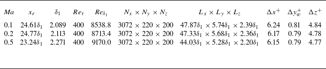

 a
 Ma=0.1
 b
 Ma=0.2
 c
 Ma=0.5

 10
 10[Φ(k1,k3,ω)]
 ωδ1/Ue=23.44(Ma=0.5)

 Ma=0.1
 k3=0
 k1=0
 kc=ω/Uc
 ωδ1/Ue=20.04
 Φ(k1,0,ω)
 k1/kc
 ωδ1/Ue=30.06
 Φ(k1,0,ω)
 k1/kc
 ωδ1/Ue=70.14
 Φ(k1,0,ω)
 k1/kc
 ωδ1/Ue=20.04
 Φ(0,k3,ω)
 k3/kc
 ωδ1/Ue=30.06
 Φ(0,k3,ω)
 k3/kc
 ωδ1/Ue=70.14
 Φ(0,k3,ω)
 k3/kc

 Ma=0.2
 k3=0
 k1=0
 kc=ω/Uc
 ωδ1/Ue=35.47
 Φ(k1,0,ω)
 k1/kc
 ωδ1/Ue=47.80
 Φ(k1,0,ω)
 k1/kc
 ωδ1/Ue=82.05
 Φ(k1,0,ω)
 k1/kc
 ωδ1/Ue=35.47
 Φ(0,k3,ω)
 k3/kc
 ωδ1/Ue=47.80
 Φ(0,k3,ω)
 k3/kc
 ωδ1/Ue=82.05
 Φ(0,k3,ω)
 k3/kc


 Ma=0.5
 k3=0
 k1=0
 kc=ω/Uc
 ωδ1/Ue=28.23
 Φ(k1,0,ω)
 k1/kc
 ωδ1/Ue=47.13
 Φ(k1,0,ω)
 k1/kc
 ωδ1/Ue=88.46
 Φ(k1,0,ω)
 k1/kc
 ωδ1/Ue=28.23
 Φ(0,k3,ω)
 k3/kc
 ωδ1/Ue=47.13
 Φ(0,k3,ω)
 k3/kc
 ωδ1/Ue=88.46
 Φ(0,k3,ω)
 k3/kc

 Ma=0.5
 ωδ1/Ue=28.23
 k3=0
 k1/kc
 kc=ω/Uc
 ±30%
 ±50%
 α11
 α22
 α33
 α
 β1
 β2
 b
 σ
 γ

 k1=0
 k3/kc

 10log10{[(F+F′)(F+F′)∗]/(4F0F0∗)}
 a
 k1/k0=0.51
 b
 k1/k0=0.79
 c
 k1/k0=0.91
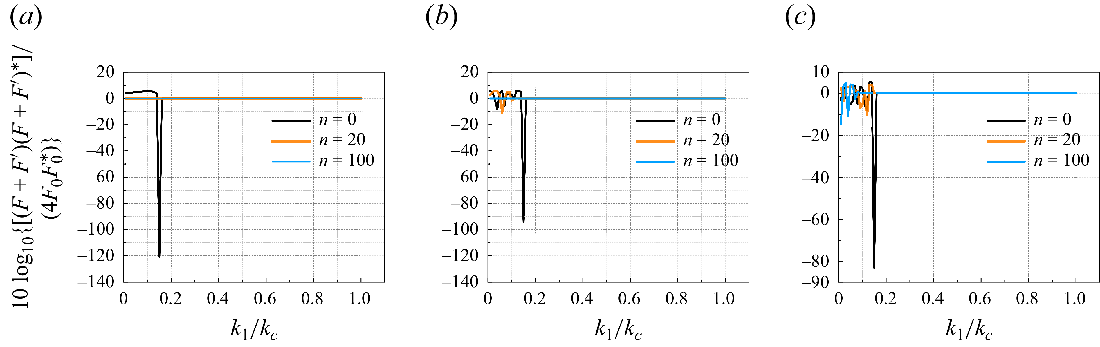
 10log10{[(F+F′)(F+F′)∗]/(4F0F0∗)}
 k1/kc
 a
 ω=500
 b
 ω=1000
 c
 ω=40000

 10log10(4FF∗)
 a
 k1/k0=0.51
 b
 k1/k0=0.79
 c
 k1/k0=0.91
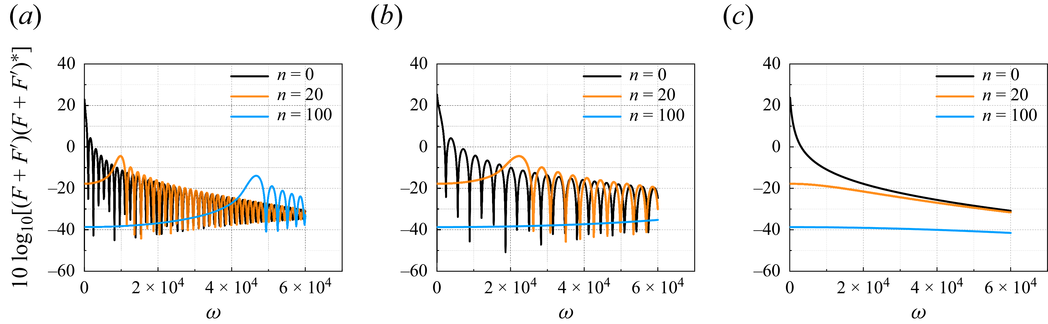
 10log10[(F+F′)(F+F′)∗]
 a
 k1/k0=0.51
 b
 k1/k0=0.79
 c
 k1/k0=0.91
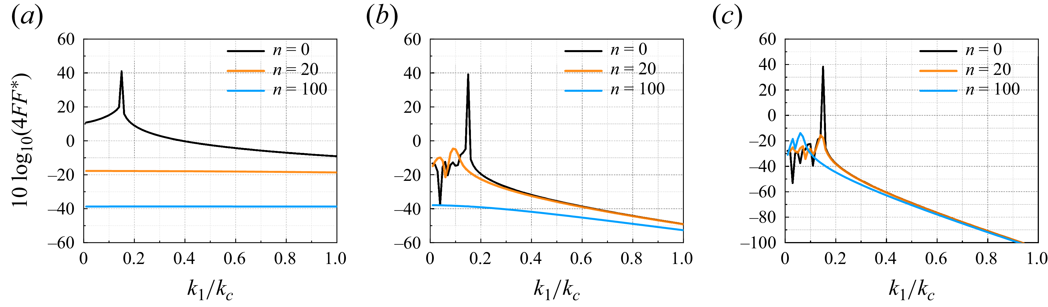
 10log10(4FF∗)
 k1/kc
 a
 ω=500
 b
 ω=1000
 c
 ω=40000
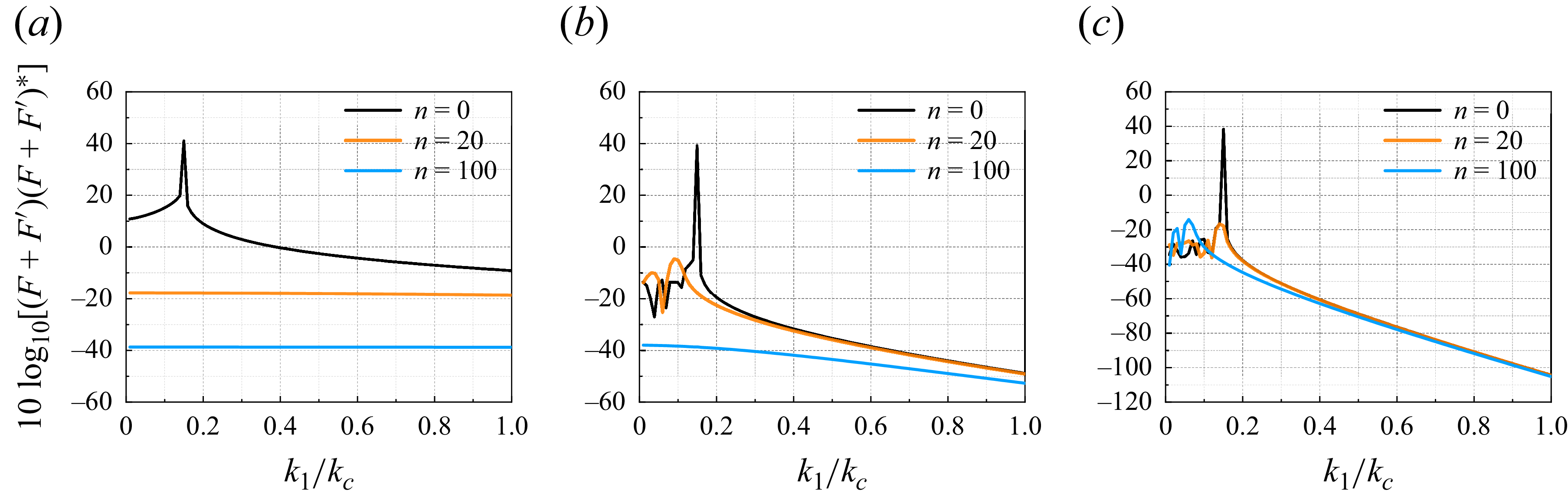
 10log10[(F+F′)(F+F′)∗]
 k1/kc
 a
 ω=500
 b
 ω=1000
 c
 ω=40000
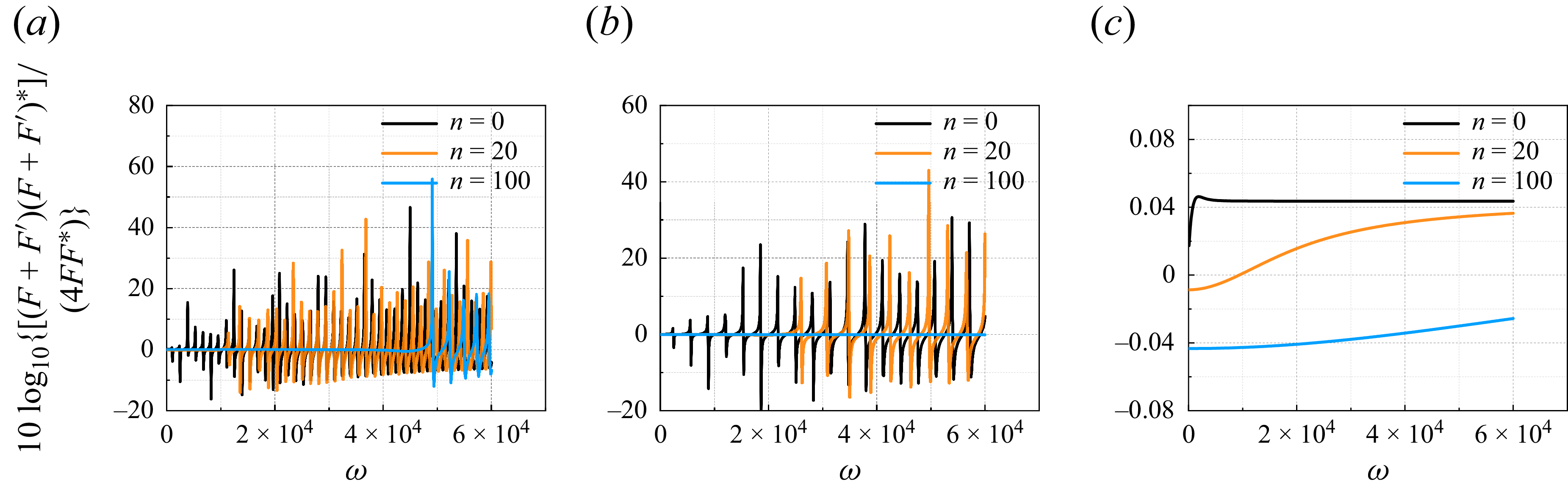
 10log10{[(F+F′)(F+F′)∗]/(4FF∗)}
 a
 k1/k0=0.51
 b
 k1/k0=0.79
 c
 k1/k0=0.91
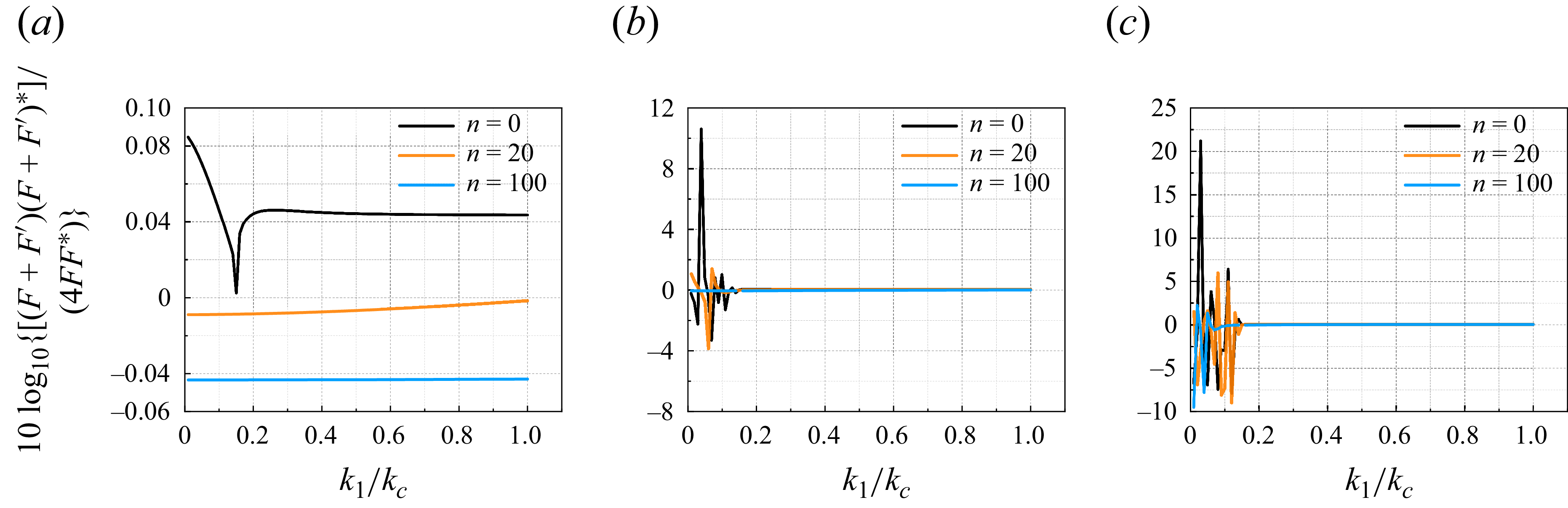
 10log10{[(F+F′)(F+F′)∗]/(4FF∗)}
 k1/kc
 a
 ω=500
 b
 ω=1000
 c
 ω=40000

 10log10[(F+F′)(F+F′)∗]
 a
 ω=500
 b
 ω=1000
 c
 ω=40000


