1. Introduction
Artificial microswimmers have been drawing increasing attention in the past decades, driven by various potential applications such as targeted drug delivery (Ma et al. Reference Ma2022) and decontamination (Li et al. Reference Li, Wu, Xiong, Liang, Li, Liu, Cao, Wang, Tang and Li2022). They are propelled either by external energy sources like magnetic or electric fields (Han et al. Reference Han, Zhu, Shaevitz and Stone2021; Martín-Roca et al. Reference Martín-Roca, Ortega, Valeriani, Rubio and Martínez-Pedrero2023), or by local energy sources due to chemical reactions. A typical example of the latter is given by phoretic particles (including rigid particles and droplets), which can swim due to phoretic flows resulting from surface solute concentration gradients or Marangoni flows resulting from surface tension gradients induced by local surfactant concentration (Michelin Reference Michelin2023). The concentration gradients can be created by asymmetric properties of the particle’s surface, as happens for Janus particles (Paxton et al. Reference Paxton, Kistler, Olmeda, Sen, St. Angelo, Cao, Mallouk, Lammert and Crespi2004). It was further shown that an isotropic particle was able to generate concentration gradients, activating a spontaneous autophoretic directed motion (Michelin, Lauga & Bartolo Reference Michelin, Lauga and Bartolo2013; Izri et al. Reference Izri, van der Linden, Michelin and Dauchot2014; Michelin & Lauga Reference Michelin and Lauga2014).
Recent studies have been devoted to elucidating the more complex dynamics of phoretic particles driven by the nonlinear coupling between hydrodynamic and chemical fields. For a phoretic particle in infinite fluid, transition to unsteady and chaotic motions is found numerically and theoretically with increasing advection (Hu et al. Reference Hu, Lin, Rafai and Misbah2019; Farutin et al. Reference Farutin, Rizvi, Hu, Lin, Rafaï and Misbah2022; Li Reference Li2022). The flow and solute concentration are affected by freely swimming particles and fixed boundaries, so that a particle can be trapped by trajectories of other particles and large pillars (Jin et al. Reference Jin, Vachier, Bandyopadhyay, Macharashvili and Maass2019; Izzet et al. Reference Izzet, Moerman, Gross, Groenewold, Hollingsworth, Bibette and Brujic2020). The interaction among multiple particles might lead to collective behaviours such as travelling lines, dynamic crystallites (Thutupalli et al. Reference Thutupalli, Geyer, Singh, Adhikari and Stone2018), caging (Hokmabad et al. Reference Hokmabad, Agudo-Canalejo, Saha, Golestanian and Maass2022a ), rotating clusters (Hokmabad et al. Reference Hokmabad, Nishide, Ramesh, Kruger and Maass2022b ) and active turbulence (Yang et al. Reference Yang, Jiang, Picano and Zhu2024). In order to study these complex dynamics, a general numerical framework is needed. This constitutes the main motivation of the present work.
Numerical modelling of phoretic particles is not a trivial task, due to the nonlinear character of the solute advection by the fluid flows as well as to the presence of moving boundary conditions. Most numerical frameworks are designed for specific problems, which either deal with simple geometries or simplified models. For simple geometric configurations like the case of a single particle in an unconfined domain or the case of two-particle interactions, the full coupling of flow and solute field can be resolved using polar coordinates (Michelin et al. Reference Michelin, Lauga and Bartolo2013; Michelin & Lauga Reference Michelin and Lauga2014; Sondak et al. Reference Sondak, Hawley, Heng, Vinsonhaler, Lauga and Thiffeault2016) or bi-polar coordinates (Lippera et al. Reference Lippera, Morozov, Benzaquen and Michelin2020; Desai & Michelin Reference Desai and Michelin2021). However, this does not apply to the case of more particles or to the case of a confined geometry, like in the presence of bounding walls (e.g. straight channels). To investigate collective behaviours for multiple particles, simplified models have been used. A simplification consisted of considering the particles as point sources (Lippera, Benzaquen & Michelin Reference Lippera, Benzaquen and Michelin2021), instead of being of finite size. Another simplification considered the case of rapid diffusion and rapid viscous transport (Montenegro-Johnson, Michelin & Lauga Reference Montenegro-Johnson, Michelin and Lauga2015; Singh, Adhikari & Cates Reference Singh, Adhikari and Cates2019; Rojas-Pérez et al. Reference Rojas-Pérez, Delmotte and Michelin2021). In these simplified models, the nonlinear advection term is discarded, and the solute transport reduces to either unsteady diffusion or Laplace problems. For these simplified models, several fast numerical methods have been developed recently to deal with suspensions of phoretic particles (Yan & Shelley Reference Yan and Shelley2018; Kohl et al. Reference Kohl, Corona, Cheruvu and Veerapaneni2023; Delmotte & Usabiaga Reference Delmotte and Usabiaga2024). However, without the nonlinear advection term, some collective behaviours driven by the nonlinear coupling between hydrodynamic and chemical fields cannot be reproduced, such as particle attraction (Jin et al. Reference Jin, Vachier, Bandyopadhyay, Macharashvili and Maass2019; Hokmabad et al. Reference Hokmabad, Nishide, Ramesh, Kruger and Maass2022b ) and active turbulence (Yang et al. Reference Yang, Jiang, Picano and Zhu2024). Recently, some efforts have been directed towards accounting for more general geometries, larger numbers of particles and nonlinearity of solute advection. By combining the embedded boundary method (EBM) with adaptive mesh refinement, the self-propulsion of an isotropic active particle in cylindrical pipes have been studied (Picella & Michelin Reference Picella and Michelin2022). Others studies used the immersed boundary method (IBM) for both flow and solute field (Chen et al. Reference Chen, Chong, Liu, Verzicco and Lohse2021; Yang et al. Reference Yang, Jiang, Picano and Zhu2024), which transfers sharp boundary problems into diffuse boundary problems.
A full numerical framework for phoretic particles consists of two parts: the Stokes flow and the advection–diffusion problem for solute, which both contain moving boundaries. As particle motions are determined by solute distributions on their surfaces (Michelin et al. Reference Michelin, Lauga and Bartolo2013), the key point is to resolve boundary conditions on these moving boundaries. For the Stokes flow, the moving boundary problem can be solved by Green’s function, also known as boundary integral method (BIM) (Pozrikidis Reference Pozrikidis1992). However, most boundary integral based methods are not appropriate for the present study due to following reasons. First, as the solute is advected by the flow, the boundary integral equation should be calculated on all sampling points in the fluid domain, not just on boundaries. Second, with the increase of particle numbers, the computational complexity scales as
 $O(N^2)$
, where
 $N$
is proportional to the product of the number of particles and the number of sampling points on each particle. To overcome these limitations, several accelerated techniques have been developed, such as the particle–particle–particle–mesh method (Deserno & Holm Reference Deserno and Holm1998), the particle–mesh–Ewald (PME) method (Essmann et al. Reference Essmann, Perera, Berkowitz, Darden, Lee and Pedersen1995; Guckel Reference Guckel1999), the fast multipole method (Yan & Shelley Reference Yan and Shelley2018) and general geometry Ewald-like method (GGEM) (Hernandez-Ortiz, de Pablo & Graham Reference Hernandez-Ortiz, de Pablo and Graham2007; Kumar & Graham Reference Kumar and Graham2012).
There are other numerical techniques for simulating fluid flow and advection–diffusion problems with moving boundaries. One candidate is the EBM or the cut-cell method, by which the Cartesian meshes are cut and reconstructed by moving boundaries (McCorquodale, Colella & Johansen Reference McCorquodale, Colella and Johansen2001; Schneiders et al. Reference Schneiders, Günther, Meinke and Schröder2016). The reconstructed meshes are body fitted in the vicinity of boundaries, which provide sharp resolution of boundaries and interfaces, while the remainder remain fixed Cartesian meshes. The overlapping mesh method (OMM) employs body-fitted meshes to several overlapping subdomains, and interpolates values on subdomain interfaces (Chesshire & Henshaw Reference Chesshire and Henshaw1990; Henshaw & Schwendeman Reference Henshaw and Schwendeman2008). Moreover, it allows these decomposed subdomains to move independently, suitable for moving boundary problems (Prewitt, Belk & Shyy Reference Prewitt, Belk and Shyy2000; Henshaw & Schwendeman Reference Henshaw and Schwendeman2006; Merrill & Peet Reference Merrill and Peet2019). Another popular technique is the IBM (Goldstein, Handler & Sirovich Reference Goldstein, Handler and Sirovich1993; Peskin Reference Peskin2002; Wang et al. Reference Wang, Gong, Sugiyama, Takagi and Huang2020). Boundary conditions are considered as source terms, and are spread to neighbouring mesh points with a smoothed delta function, creating a smeared interface with finite thickness. To obtain sharp interfaces, the immersed interface method applies interpolation or extrapolation to derive approximate boundary values or normal derivatives on neighbouring mesh points (Li & Lai Reference Li and Lai2001; Hu, Lai & Misbah Reference Hu, Lai and Misbah2018). Similar ideas are applied to lattice Boltzmann method (LBM) as modified bounce-back boundary conditions (Lallemand & Luo Reference Lallemand and Luo2003; Huang, Hu & Yong Reference Huang, Hu and Yong2016; Zhang & Misbah Reference Zhang and Misbah2019). Last but not least, particle-based methods are also used for studies of moving boundary problems, such as multiparticle collision dynamics (Noguchi & Gompper Reference Noguchi and Gompper2004, Reference Noguchi and Gompper2005), dissipative particle dynamics (Fedosov, Caswell & Karniadakis Reference Fedosov, Caswell and Karniadakis2010; Gao et al. Reference Gao, Zhang, Marom, Deng and Bluestein2017; Xu et al. Reference Xu, Wang, He, Hao and Zhang2023) and smoothed particle hydrodynamics (Tanaka & Takano 2005; Hosseini & Feng Reference Hosseini and Feng2009), to name but a few.
In preliminary studies, we first attempted to modify an IBM-based framework (Zhang et al. Reference Zhang, Shen, Hogan, Barakat and Misbah2018; Gou et al. Reference Gou, Zhang, Abbasi and Misbah2021) to model phoretic particles numerically. The Stokes flow was solved using the combined immersed boundary–lattice Boltzmann method (Shen et al. Reference Shen, Farutin, Thiebaud and Misbah2017). To account for low inertial effect, the Reynolds number was set to 0.05. The LBM with modified bounce-back boundary condition was employed for the advection and diffusion of solute (Zhang & Misbah Reference Zhang and Misbah2019). Although this IBM-based framework could reproduce the symmetry breaking from stationary to straight motion for a circular phoretic particle, we found that the critical Péclet number
 $Pe$
for straight motion was smaller (within 5 %–10
 $\%$
) than the analytical finding (Hu et al. Reference Hu, Lin, Rafai and Misbah2019). Here,
 $Pe$
is the ratio of advection and diffusion. Moreover, we could obtain only qualitative agreement for meandering, circular and chaotic motions. Further analysis showed that the IBM and the modified bounce-back boundary condition were only first-order accurate on the particle’s surface. In fact, quantitative disagreements have been observed in other studies (Chen et al. Reference Chen, Chong, Liu, Verzicco and Lohse2021; Yang et al. Reference Yang, Jiang, Picano and Zhu2024; Zhu et al. Reference Zhu, Chen, Chong, Lohse and Verzicco2024) when using IBM-based methods. For a circular phoretic particle, the critical
 $Pe$
for straight motion was also smaller than the benchmark in Yang et al. (Reference Yang, Jiang, Picano and Zhu2024), and the phoretic velocity was slightly overestimated. For a spherical phoretic particle, chaotic motion was reported for
 $Pe \gt 15$
in Chen et al. (Reference Chen, Chong, Liu, Verzicco and Lohse2021), while a more accurate result should be
 $Pe \geqslant 24.2$
(Lin, Hu & Misbah Reference Lin, Hu and Misbah2020; Hu et al. Reference Hu, Lin, Rafai and Misbah2022). Further studies showed that the order of convergence is around 1.31 (Zhu et al. Reference Zhu, Chen, Chong, Lohse and Verzicco2024), in agreement with our preliminary studies. These works indicate that a better alternative for the IBM should be proposed for quantitative studies of phoretic particles.
In this work, we develop a computational framework to resolve precisely the multiparticle dynamics in periodic or confined domains, which is seldom reported in literature. For the fluid flow, we propose a fast boundary integral method (FBIM) for arbitrary geometries, inspired by the GGEM (Hernandez-Ortiz et al. Reference Hernandez-Ortiz, de Pablo and Graham2007). The FBIM combines the advantages of BIM and IBM, being sufficiently efficient and accurate at the same time. For the advection–diffusion problem, we employ an OMM with second-order accuracy in space. The subdomains attached to particles can move freely in the background fluid domain, resolving moving boundary conditions. The rest of this paper is organised as follows. In § 2, we first recall the governing equations for the motion of phoretic particles. Then we present the numerical implementation of the FBIM, the rigid body dynamics and the OMM in §§ 3, 4 and 5, respectively. The solution procedure is presented in § 6. In § 7, the FBIM and the OMM are validated separately, and convergence studies are performed. Lastly, the combined FBIM-OMM is employed to solve several general problems in § 8, and the effects of confined geometries and multiparticle interactions are explored.
2. Problem formulation
We consider a two-dimensional (2-D) computational domain
 $C$
of circular particles of radius
 $a$
immersed in a Newtonian fluid of viscosity
 $\mu$
. These particles are chemically active and can emit or absorb a solute into the surrounding fluid with an isotropic flux
 $\mathcal{A}$
. The solute diffuses with a molecular diffusivity
 $\mathcal{D}$
and is advected by the fluid flow. A chemical reaction could consume or produce the solute in this domain, and the reaction rate is proportional to the local solute concentration with coefficient
 $\mathcal{B}$
. The interaction of the solute molecules with the particles induces a slip tangential flow on the particle surfaces with a mobility
 $\mathcal{M}$
(Michelin & Lauga Reference Michelin and Lauga2014).
In the following, we adopt the non-dimensionalisation of Michelin et al. (Reference Michelin, Lauga and Bartolo2013) where the length, fluid velocity, the solute concentration and the pressure (or stress) are scaled by the characteristic values
 $a$
,
 $|\mathcal{AM}|/\mathcal{D}$
,
 $a|\mathcal{A}|/\mathcal{D}$
and
 $\mu |\mathcal{AM}|/a\mathcal{D}$
, respectively. The governing equations in dimensionless form are
 \begin{align}&\qquad\qquad \nabla p(\boldsymbol{x}, t) = \nabla ^2 \boldsymbol{u}(\boldsymbol{x}, t), \boldsymbol{\nabla} \boldsymbol{\cdot} \boldsymbol{u}(\boldsymbol{x}, t) = 0, \end{align}
 \begin{align}& \frac {\partial c(\boldsymbol{x}, t)}{\partial t} + \boldsymbol{u}(\boldsymbol{x}, t) \boldsymbol{\cdot} \boldsymbol{\nabla} c(\boldsymbol{x}, t) = \frac {1}{Pe} \nabla ^2 c(\boldsymbol{x}, t) - \beta c(\boldsymbol{x}, t), \end{align}
where
 $p$
,
 $\boldsymbol{u}$
and
 $c$
are the dimensionless fluid pressure, velocity and solute concentration,
 $Pe = a|\mathcal{AM}|/\mathcal{D}^2$
is the Péclet number which describes the ratio of advection and diffusion over the transport of solute and
 $\beta = a\mathcal{BD}/|\mathcal{AM}|$
is the dimensionless consumption/production coefficient.
At the surface of a particle
 $ \Gamma _p$
or a fixed boundary
 $ \Gamma _f$
, the boundary conditions for the flow and the concentration field read
 \begin{align}& \boldsymbol{u}(\boldsymbol{x}, t)|_{ \Gamma _p} = M \nabla _s c(\boldsymbol{x}, t)|_{ \Gamma _p} + \boldsymbol{U}_{\!\!p}(t) + \boldsymbol{ \Omega }_p(t) \times (\boldsymbol{x} - \boldsymbol{X}_{\!p}), \boldsymbol{u}(\boldsymbol{x}, t)|_{ \Gamma _f} = \boldsymbol{0}, \end{align}
 \begin{align}&\qquad\qquad\qquad\quad \boldsymbol{n} \boldsymbol{\cdot} \boldsymbol{\nabla} c(\boldsymbol{x}, t)|_{ \Gamma _p} = - A, \boldsymbol{n} \boldsymbol{\cdot} \boldsymbol{\nabla} c(\boldsymbol{x}, t)|_{ \Gamma _f} = 0, \end{align}
where
 $\boldsymbol{U}_{\!\!p} = U_{p_x} \boldsymbol{e}_x + U_{p_y} \boldsymbol{e}_y$
and
 $\boldsymbol{ \Omega }_p = \Omega _p \boldsymbol{e}_z$
are the translational and rotational velocities of the particle, with
 $\boldsymbol{e}_z = \boldsymbol{e}_x \times \boldsymbol{e}_y$
,
 $\boldsymbol{X}_{\!p}$
is the centre of the particle,
 $\nabla _s$
is the surface gradient operator,
 $\boldsymbol{n}$
is the unit outward normal,
 $M = \mathcal{M}/|\mathcal{M}|$
is the dimensionless mobility and
 $A = \mathcal{A}/|\mathcal{A}|$
is the dimensionless activity. Here, positive
 $ \Omega _p$
corresponds to counterclockwise rotation, and vice versa. In order to trigger self-propulsion in infinite fluid,
 $A$
and
 $M$
must have the same sign (Michelin et al. Reference Michelin, Lauga and Bartolo2013; Hu et al. Reference Hu, Lin, Rafai and Misbah2019). The particle moves as a rigid body, and its centre
 $\boldsymbol{X}_{\!p}$
and orientation angle
 $ \Theta _p$
are given by
 \begin{equation} \frac {{\rm d}\boldsymbol{X}_{\!p}}{{\rm d}t} = \boldsymbol{U}_{\!\!p}(t), \frac {{\rm d} \Theta _p}{{\rm d}t} = \Omega _p(t). \end{equation}
In the Stokes regime, there are two other constraints on each particle in the absence of external force: the force-free and torque-free conditions. For a phoretic particle, the total force applied to it is the sum of the hydrodynamic force on its surface and the interaction forces with the solute molecules in the entire fluid domain. In this work, we adopt the thin-interaction-layer limit that the interaction force is negligible if
 $|\boldsymbol{x} - \boldsymbol{X}_{\!p}| - 1 \gg \lambda$
and
 $\lambda \ll 1$
, where
 $\lambda$
is the interaction range. In this thin-interaction-layer limit, this is equivalent to imposing the zero hydrodynamic force and torque conditions on the outer boundary of the interaction layer, which is approximately the particle’s surface. For this reason, we impose the following force-free and torque-free conditions:
 \begin{equation} \int _{ \Gamma _p} \boldsymbol{\sigma }(\boldsymbol{x}, t) \boldsymbol{\cdot} \boldsymbol{n} {\rm d}S(\boldsymbol{x}) = \boldsymbol{0}, \int _{ \Gamma _p} (\boldsymbol{x} - \boldsymbol{X}_{\!p}) \times \left [ \boldsymbol{\sigma }(\boldsymbol{x}, t) \boldsymbol{\cdot} \boldsymbol{n} \right ] {\rm d}S(\boldsymbol{x}) = \boldsymbol{0}, \end{equation}
where
 $\boldsymbol{\sigma } = -p \boldsymbol{I} + \nabla \boldsymbol{u} + \nabla \boldsymbol{u}^T$
is the flow stress tensor, and
 $S$
is the curvilinear coordinate on the particle boundary
 $ \Gamma _p$
.
3. Fast boundary integral method for fluid
The implementation of the FBIM is given as follows. We first recall the boundary integral equation, and then derive the analytical solution due to a point force based on Ewald-like decomposition. Later, we apply the decomposed solution to calculate the single-layer integral on boundaries.
3.1. Boundary integral equation
The flow field is described by the Stokes equation (2.1) with Dirichlet boundary conditions (2.3). A general solution can be obtained by the boundary integral equation (Pozrikidis Reference Pozrikidis1992)
 \begin{equation} u_i(\boldsymbol{x}) = \frac {1}{4 \pi } \sum _{n=1}^{N_b} \int _{ \Gamma _n} G_{ij}(\boldsymbol{x}, \boldsymbol{X}) F_j(\boldsymbol{X}) {\rm d}S(\boldsymbol{X}), \end{equation}
where
 $ \Gamma _n$
is the contour of the
 $n$
th boundary,
 $\boldsymbol{X}$
is a point on this boundary,
 $\boldsymbol{G}$
is the 2-D Green’s function,
 $\boldsymbol{F}$
is the surface force density to enforce the boundary conditions (2.3) on
 $ \Gamma _n$
and the summations are over all the
 $N_b$
boundaries. For an infinite domain, the free-space Green’s function (Pozrikidis Reference Pozrikidis1992) is used as
 \begin{equation} G_{ij}(\boldsymbol{x}, \boldsymbol{x}') = -\delta _{ij} \ln (|\boldsymbol{x} - \boldsymbol{x}'|) + \frac {(x_i - x'_i) (x_{\!j} - x'_{\!j})}{|\boldsymbol{x} - \boldsymbol{x}'|^2}. \end{equation}
The FBIM is derived based on (3.1) and (3.2).
It should be noted that (3.1) is the generalised single-layer representation (Pozrikidis Reference Pozrikidis1992). For a phoretic particle with slip velocity,
 $\boldsymbol{F}$
is not the surface traction applied to the fluid (which equals to
 $- \boldsymbol{\sigma } \boldsymbol{\cdot} \boldsymbol{n}$
), but a fictitious force to enforce the velocity boundary condition on its surface
 $ \Gamma _p$
. Nevertheless, it still satisfies force-free and torque-free conditions (Pozrikidis Reference Pozrikidis1992), which will be used later to calculate the rigid particle dynamics.
(a) Schematic of the point force at
 $\boldsymbol{x}^v$
and the near neighbour region
 $C_c$
. (b) Long-range density
 $D^l$
(see (3.11)) as a function of
 $r$
. Here, the cutoff distance is set as
 $r_c = 4$
.

3.2. Decomposed solution due to a point force
We start from the simplest case, which is the flow due to a point force
 \begin{equation} \nabla p(\boldsymbol{x}) = \nabla ^2 \boldsymbol{u}(\boldsymbol{x}) + \boldsymbol{g}^v\delta (|\boldsymbol{x} - \boldsymbol{x}^v|), \boldsymbol{\nabla} \boldsymbol{\cdot} \boldsymbol{u}(\boldsymbol{x}) = 0, \end{equation}
where
 $\boldsymbol{g}^v$
is the force applied at a point
 $\boldsymbol{x}^v$
(see figure 1
a). The resulting velocity is
 \begin{equation} u_i(\boldsymbol{x}) = \frac {1}{4 \pi } G_{ij}(\boldsymbol{x}, \boldsymbol{x}^v) g_j^v. \end{equation}
Inspired by other Ewald-summation-based methods (Essmann et al. Reference Essmann, Perera, Berkowitz, Darden, Lee and Pedersen1995; Guckel Reference Guckel1999; Hernandez-Ortiz et al. Reference Hernandez-Ortiz, de Pablo and Graham2007), the idea of the FBIM is to split the Dirac-delta density
 $\delta (r)$
in (3.3) into a sum of a short-range density
 $D^s(r)$
containing the singularity, and a sufficiently smooth long-range density
 $D^l(r) = \delta (r) - D^s(r)$
. Here,
 $r$
refers to the magnitude of the vector from any position to the pole of singularity,
 $\boldsymbol{r} = \boldsymbol{x} - \boldsymbol{x}^v$
. The short-range density is chosen in such a way that, for any point beyond a certain cutoff distance
 $r_c$
(i.e.
 $r \gt r_c$
), the flow velocity due to the short-range force density
 $\boldsymbol{g}^v D^s(r)$
is zero.
The solution of the Stokes and continuity equation is also decomposed into two parts. For the long-range part, the solution
 $\boldsymbol{u}^l(\boldsymbol{x})$
and
 $p^l(\boldsymbol{x})$
due to the long-range force density satisfies the following set of equations:
 \begin{equation} \nabla p^l(\boldsymbol{x}) = \nabla ^2 \boldsymbol{u}^l(\boldsymbol{x}) + \boldsymbol{g}^v D^l(|\boldsymbol{x} - \boldsymbol{x}^v|), \boldsymbol{\nabla} \boldsymbol{\cdot} \boldsymbol{u}^l(\boldsymbol{x}) = 0. \end{equation}
This equation can be solved by any Stokes solver, and we will use a Fourier spectral method in this study. The short-range solution
 $\boldsymbol{u}^s(\boldsymbol{x})$
and
 $p^s(\boldsymbol{x})$
satisfies the short-range set of equations
 \begin{equation} \nabla p^s(\boldsymbol{x}) = \nabla ^2 \boldsymbol{u}^s(\boldsymbol{x}) + \boldsymbol{g}^v D^s(|\boldsymbol{x} - \boldsymbol{x}^v|), \boldsymbol{\nabla} \boldsymbol{\cdot} \boldsymbol{u}^s(\boldsymbol{x}) = 0. \end{equation}
This equation will be solved by using a short-range Green’s function for any points within the cutoff distance (
 $r \leqslant r_c$
). Once the two problems are solved, the overall solution is obtained as
 \begin{equation} \boldsymbol{u}(\boldsymbol{x}) = \boldsymbol{u}^l(\boldsymbol{x}) + \boldsymbol{u}^s(\boldsymbol{x}), p(\boldsymbol{x}) = p^l(\boldsymbol{x}) + p^s(\boldsymbol{x}). \end{equation}
3.2.1. Long-range solution
To solve the long-range problem, a proper long-range density
 $D^l(r)$
should be chosen. The first constraint on
 $D^l(r)$
is the finite cutoff distance
 $r_c$
, such that
 \begin{equation} D^l(r) = 0, \forall r \geqslant r_c. \end{equation}
Despite this, in order to have a smooth solution of
 $\boldsymbol{u}^l(\boldsymbol{x})$
, its derivatives should be continuous at
 $r = r_c$
as
 \begin{equation} \left . \frac {\partial ^k D^l}{\partial r^k} \right |_{r = r_c} = 0, k = 1, 2, 3, \ldots , k_{max} ,\end{equation}
where
 $k_{max}$
is the cutoff order of the derivatives.
The second constraint is related to the solution induced by the point force. As follows from the above, the solution driven by the long-range force density is the same as that driven by the point force for any point beyond the cutoff distance. Define
 $C_c$
as the near neighbour region around the singular point
 $\boldsymbol{x}^v$
within the cutoff distance
 $r_c$
(see figure 1
a), then the following equation is valid for any point
 $\boldsymbol{x} \in C \setminus C_c$
:
 \begin{equation} u_i^l(\boldsymbol{x}) = \frac {1}{4 \pi } G_{ij}(\boldsymbol{x}, \boldsymbol{x}^v) g_j ^v = \frac {1}{4 \pi } \int _{C_c} G_{ij}(\boldsymbol{x}, \boldsymbol{x}') g_j^v D^l(|\boldsymbol{x}' - \boldsymbol{x}^v|) {\rm d}\boldsymbol{x}'. \end{equation}
We found a sixth-order polynomial which satisfies the above constraints as (see figure 1 b)
 \begin{equation} D^l(r) = \left \{ \begin{aligned} &0, & r \geqslant r_c \\ &\frac {56}{3 \pi r_c^2} \left [-\frac {25}{2}\left(\frac {r}{r_c}\right)^6 + 54\left(\frac {r}{r_c}\right)^5 - 90\left(\frac {r}{r_c}\right)^4 + 70\left(\frac {r}{r_c}\right)^3 - \frac {45}{2}\left(\frac {r}{r_c}\right)^2 + 1 \right ], & r \lt r_c \end{aligned} \right . . \end{equation}
The detailed derivation is given in Appendix A. Actually, it turns out that an expansion of
 $D^l(r)$
as higher-order polynomial with only even degree terms leads to higher-order accuracy. It should be noted that the choice of long-range density is not unique. Any functions that satisfy (3.8)–(3.10) would be valid. Moreover, the long-range density
 $D^l$
is strictly equal to 0 for any point beyond the cutoff distance. This is different from the screening function in GGEM (Hernandez-Ortiz et al. Reference Hernandez-Ortiz, de Pablo and Graham2007; Kumar & Graham Reference Kumar and Graham2012) and the Hasimoto splitting (Bao et al. Reference Bao, Rachh, Keaveny, Greengard and Donev2018), which are quasi-Gaussian and decay exponentially to 0. Such kind of decomposition leads to truncation errors at the cutoff distance.
To solve (3.5), the discrete Fourier series approximation is employed in the periodic
 $x$
and
 $y$
directions. The two components of the long-range velocity
 $\boldsymbol{u}^l = (u_x^l, u_y^l)$
are expressed as
 \begin{equation} u_x^l(\boldsymbol{x}) + i u_y^l(\boldsymbol{x}) = \sum _{m = -N_x/2}^{N_x/2} \sum _{n = -N_y/2}^{N_y/2} \hat {u}_{mn}^l \textrm{e}^{i 2\pi mx/L_x} \textrm{e}^{{i} 2\pi ny/L_y}, \end{equation}
where
 $N_x$
and
 $N_y$
are the number of modes in the corresponding series approximation, and
 $\hat {u}_{mn}^l$
is the complex amplitude of the harmonic. Similarly, the long-range force density
 $\boldsymbol{f}^l(\boldsymbol{x}) = \boldsymbol{g}^v D^l(|\boldsymbol{x} - \boldsymbol{x}^v|)$
is also represented by discrete Fourier series as
 \begin{equation} f_x^l(\boldsymbol{x}) + i f_y^l(\boldsymbol{x}) = \sum _{m = -N_x/2}^{N_x/2} \sum _{n = -N_y/2}^{N_y/2} \hat {f}_{mn}^l \textrm{e}^{{i} 2\pi mx/L_x} \textrm{e}^{{i} 2\pi ny/L_y}, \end{equation}
where
 $\hat {f}_{mn}^l$
is the complex amplitude of the harmonic. The computational domain is a rectangle, and is discretised by means of equally spaced Cartesian mesh with mesh size
 $\Delta x$
. The number of mesh points in
 $x$
and
 $y$
directions are set equal to the number of Fourier modes
 $N_x$
and
 $N_y$
, respectively, so that the fast Fourier transform (FFT) can be used to transfer data between real and Fourier space. The FFT and reverse FFT are calculated by the cuFFT library (NVIDIA 2022), which is accelerated by GPU. In practice, (3.5) is first transformed into Fourier space using FFT. Then the harmonic’s amplitude
 $\hat {u}_{mn}^l$
is calculated as
 \begin{equation} \hat {u}^l_{mn} = \frac {1}{2(m^2 + n^2)} \left (\hat {f}^l_{mn} - \frac {m^2 + i2 mn - n^2}{m^2 + n^2}\hat {f}^{l*}_{-m-n} \right ), mn \neq 0, \end{equation}
where
 $\hat {f}^{l*}_{-m-n}$
is the complex conjugate of
 $\hat {f}^{l}_{-m-n}$
. The zeroth mode
 $\hat {u}^l_{00}$
corresponds to the average velocity in the computational domain, which is zero, unless there is an imposed flow (not considered here). Finally, a reverse FFT is employed to compute the long-range velocity
 $\boldsymbol{u}^l$
in real space. For any point not lying on the mesh, the velocity is obtained by bi-cubic interpolation with fourth-order accuracy in space.
3.2.2. Short-range solution
The short-range density is
 \begin{equation} D^s(r) = \delta (\boldsymbol{r}) - D^l(r). \end{equation}
The short-range velocity is then obtained as
 \begin{equation} u_i^s(\boldsymbol{x}) = \frac {1}{4 \pi } \int _{C_c} G_{ij}(\boldsymbol{x}, \boldsymbol{x}') g_j^v D^s(|\boldsymbol{x}' - \boldsymbol{x}^v|) {\rm d}\boldsymbol{x}'. \end{equation}
According to (3.11) and (3.15),
 $u_i^s(\boldsymbol{x}) = 0$
for any point
 $\boldsymbol{x} \in C \setminus C_c$
. Hence, (3.16) is solved for the points within the cutoff distance (i.e.
 $\boldsymbol{x} \in C_c$
) only. We define the short-range Green’s function as
 \begin{equation} G_{ij}^s (\boldsymbol{x}, \boldsymbol{x}^v) = \int _{C_c} G_{ij}(\boldsymbol{x}, \boldsymbol{x}') D^s(|\boldsymbol{x}' - \boldsymbol{x}^v|) {\rm d}\boldsymbol{x}'. \end{equation}
Then the short-range velocity reads
 \begin{equation} u_i^s(\boldsymbol{x}) = \frac {1}{4 \pi } g_j^v G_{ij}^s(\boldsymbol{x}, \boldsymbol{x}^v). \end{equation}
The derivation of the short-range Green’s function is given in Appendix B.
3.3. Single-layer integral
The velocity due to a boundary
 $ \Gamma$
is given by the single-layer integral according to (3.1). Applying the same decomposition as § 3.2, we rewrite this equation in the following form:
 \begin{equation} \begin{aligned} u_i(\boldsymbol{x}) &= \frac {1}{4 \pi } \int _{ \Gamma } G_{ij}(\boldsymbol{x}, \boldsymbol{X}) \left [ \int _{C} F_j(\boldsymbol{X}) \delta (\boldsymbol{x}' - \boldsymbol{X}) {\rm d}\boldsymbol{x}' \right ] {\rm d}S(\boldsymbol{X})\\ &= \frac {1}{4 \pi } \int _{ \Gamma } \left \{ \int _{C} G_{ij}(\boldsymbol{x}, \boldsymbol{x}') F_j(\boldsymbol{X}) \left [ D^l (|\boldsymbol{x}' - \boldsymbol{X}|) + D^s (|\boldsymbol{x}' - \boldsymbol{X}|) \right ] {\rm d}\boldsymbol{x}' \right \} {\rm d}S(\boldsymbol{X}). \end{aligned} \end{equation}
The contribution due to the long-range density is
 \begin{equation} u_i^l(\boldsymbol{x}) = \frac {1}{4 \pi } \int _{C} G_{ij}(\boldsymbol{x}, \boldsymbol{x}') \left [ \int _{ \Gamma } F_j(\boldsymbol{X}) D^l (|\boldsymbol{x}' - \boldsymbol{X}|) {\rm d}S(\boldsymbol{X}) \right ] {\rm d}\boldsymbol{x}', \end{equation}
and the long-range force density is
 \begin{equation} \boldsymbol{f}^l(\boldsymbol{x}) = \int _{ \Gamma } \boldsymbol{F}(\boldsymbol{X}) D^l (|\boldsymbol{x} - \boldsymbol{X}|) {\rm d}S(\boldsymbol{X}). \end{equation}
Next, the contribution due to the short-range density is
 \begin{equation} \begin{aligned} u_i^s(\boldsymbol{x}) &= \frac {1}{4 \pi } \int _{ \Gamma } F_j(\boldsymbol{X}) \left [ \int _{C} G_{ij}(\boldsymbol{x}, \boldsymbol{x}') D^s (|\boldsymbol{x}' - \boldsymbol{X}|) {\rm d}\boldsymbol{x}' \right ] {\rm d}S(\boldsymbol{X})\\ &= \frac {1}{4 \pi } \int _{ \Gamma } F_j(\boldsymbol{X}) G_{ij}^s(\boldsymbol{x}, \boldsymbol{X}) {\rm d}S(\boldsymbol{X}). \end{aligned} \end{equation}
Here, we describe the numerical implementation of the above problems. The surface
 $ \Gamma$
is discretised into
 $N_e$
elements. For the long-range problem, we first need to know the long-range force density
 $\boldsymbol{f}^l$
by computing the integral in (3.21). Its discretised form is written as
 \begin{equation} \boldsymbol{f}^l (\boldsymbol{x}) = \sum _{k = 1}^{N_e} \int _{ \Gamma _k} \boldsymbol{F}(\boldsymbol{X}) D^l (|\boldsymbol{x} - \boldsymbol{X}|) {\rm d}S(\boldsymbol{X}), \end{equation}
where
 $ \Gamma _k$
denotes the
 $k$
th element. The above integral can be evaluated by a simple trapezoidal rule. Then the long-range velocity
 $\boldsymbol{u}^l$
is solved for as described in § 3.2. For the short-range problem, the boundary integral in (3.22) is discretised as
 \begin{equation} \boldsymbol{u}^s (\boldsymbol{x}) = \frac {1}{4 \pi } \sum _{ \Gamma _k \in C_c} \int _{ \Gamma _k} \boldsymbol{F}(\boldsymbol{X}) \boldsymbol{G}^s (\boldsymbol{x}, \boldsymbol{X}) {\rm d}S(\boldsymbol{X}). \end{equation}
As the integrand in (3.24) includes logarithmic singularity at boundaries
 $\boldsymbol{x} = \boldsymbol{X}$
, a special quadrature rule (Crow Reference Crow1993) is used to ensure sufficient accuracy. It should be noted that the summation in (3.24) is calculated over elements within the near neighbour region of
 $\boldsymbol{x}$
, i.e.
 $ \Gamma _k \in C_c$
. The contribution of other elements has been included in the long-range solution.
4. Rigid body dynamics
In the present study, particles and geometric boundaries are considered as rigid bodies. The calculation of force and rigid body motion (translation and rotation) is given in this section.
4.1. Feedback force
The surface force density
 $\boldsymbol{F}$
to enforce boundary conditions on rigid bodies can be calculated by considering them as elastic bodies with a large elastic modulus. An alternative method is to apply a feedback force (Goldstein et al. Reference Goldstein, Handler and Sirovich1993) as
 \begin{equation} \boldsymbol{F}(\boldsymbol{X}, t) = \int _0^t \alpha \left [ \boldsymbol{V}(\boldsymbol{X}, t') - \boldsymbol{u}(\boldsymbol{X}, t') \right ] {\rm d}t', \end{equation}
so that the desired velocity
 $\boldsymbol{V}$
is enforced on the boundary. Here,
 $\alpha$
is a positive coefficient. The value of
 $\alpha$
is flow dependent, and there is not a general rule for its determination (Fadlun et al. Reference Fadlun, Verzicco, Orlandi and Mohd-Yusof2000). On the one hand,
 $\alpha$
should be large enough to enforce the boundary velocity
 $\boldsymbol{V}$
. On the other hand, big values of
 $\alpha$
increase the stiffness of (4.1) and very small time steps are required for time integration. In practice, we found that
 $\alpha \sim 10^2-10^4$
could guarantee boundary conditions for all cases simulated in the present work.
In numerical application, the time integral in (4.1) is computed in an iterative form as
 \begin{equation} \boldsymbol{F}(\boldsymbol{X}, t + \Delta t) = \boldsymbol{F}(\boldsymbol{X}, t) + \alpha \left [ \boldsymbol{V}(\boldsymbol{X}, t + \Delta t) - \boldsymbol{u}(\boldsymbol{X}, t) \right ] \Delta t, \end{equation}
where
 $\Delta t$
is the time increment. The desired velocity
 $\boldsymbol{V}(\boldsymbol{X}, t + \Delta t)$
in (4.2) depends on the boundary conditions (2.3), and might be unknown a priori. For a fixed boundary with no-slip boundary condition,
 $\boldsymbol{V} = \boldsymbol{0}$
. For a freely moving circular phoretic particle,
 $\boldsymbol{V}(\boldsymbol{X}, t + \Delta t)$
is the summation of the slip velocity, rigid body translation and rotation
 \begin{equation} \boldsymbol{V}(\boldsymbol{X}, t + \Delta t) = M \nabla _s c(\boldsymbol{X}, t + \Delta t) + \boldsymbol{U}_{\!\!p}(t + \Delta t) + \boldsymbol{ \Omega }_p(t + \Delta t) \times (\boldsymbol{X} - \boldsymbol{X}_{\!p}). \end{equation}
Here,
 $\nabla _s c(\boldsymbol{X}, t + \Delta t)$
is known once the advection–diffusion equation is solved, while
 $\boldsymbol{V}(\boldsymbol{X}, t + \Delta t)$
,
 $\boldsymbol{U}_{\!\!p}(t + \Delta t)$
and
 $\boldsymbol{ \Omega }_p(t + \Delta t)$
are unknown, and need to be solved for together with
 $\boldsymbol{F}(\boldsymbol{X}, t + \Delta t)$
. To do so, we need the following force-free and torque-free conditions:
 \begin{equation} \int _{ \Gamma _p} \boldsymbol{F}(\boldsymbol{X}) {\rm d}S(\boldsymbol{X}) = \boldsymbol{0}, \int _{ \Gamma _p} (\boldsymbol{X} - \boldsymbol{X}_{\!p}) \times \boldsymbol{F}(\boldsymbol{X}) {\rm d}S(\boldsymbol{X}) = \boldsymbol{0}. \end{equation}
The phoretic velocities
 $\boldsymbol{U}_{\!\!p}(t + \Delta t)$
and
 $\boldsymbol{ \Omega }_p(t + \Delta t)$
can be solved for by substituting (4.2) and (4.3) into (4.4) as (see Appendix C)
 \begin{align}& \boldsymbol{U}_{\!\!p}(t + \Delta t) = \frac {1}{2 \pi } \int _{ \Gamma _p} \left [ \boldsymbol{u}(\boldsymbol{X}, t) - M \nabla _s c(\boldsymbol{X}, t + \Delta t) \right ] {\rm d}S(\boldsymbol{X}),\\[-10pt]\nonumber \end{align}
 \begin{align}&\qquad \boldsymbol{ \Omega }_p(t + \Delta t) = \frac {1}{2 \pi } \int _{ \Gamma _p} (\boldsymbol{X} - \boldsymbol{X}_{\!p}) \times \boldsymbol{u}(\boldsymbol{X}, t) {\rm d}S(\boldsymbol{X}). \end{align}
Equations (4.5) and (4.6) coincide with relations between the slip velocity and the swimming velocity (identifying
 $M \nabla _s c$
with the slip velocity and
 $\boldsymbol{u}$
with the external flow) that can be derived for a single circular particle in an unbounded fluid using the reciprocal theorem (Stone & Samuel Reference Stone and Samuel1996; Elfring Reference Elfring2015). In this study, these relations continue to be applicable for an arbitrary arrangement of circular particles and rigid boundaries due to the use of the iterative procedure and the non-local nature of the boundary integral equations, which lead to a tensorial relation between the slip velocity
 $M \nabla _s c$
and the swimming velocity
 $\boldsymbol{U}_{\!\!p}$
and
 $\boldsymbol{ \Omega _p}$
, as discussed in Appendix C.
It should be noted that (4.5) and (4.6) are only valid for a circular particle of radius 1. For general case (i.e. an arbitrarily shaped particle and a circular particle of radius
 $a$
), the solution is given in Appendix C. Then
 $\boldsymbol{F}(\boldsymbol{X}, t + \Delta t)$
and
 $\boldsymbol{V}(\boldsymbol{X}, t + \Delta t)$
are calculated by (4.2) and (4.3), respectively.
4.2. Pre-conditioner
For circular particles, pre-conditioning is applied for better convergence. The idea is to approximately solve the linear system (4.2), (4.3) and (4.4) in Fourier space, considering only the hydrodynamic self-interactions of each particle independently. Its derivation is given as follows.
In a polar coordinate system
 $(1, \theta )$
attached to the particle’s centre
 $\boldsymbol{X}_{\!p}$
, the surface force
 $\boldsymbol{F}[\boldsymbol{X}(\theta )]$
, the surface velocity
 $\boldsymbol{u}[\boldsymbol{X}(\theta )]$
and the surface concentration
 $c[\boldsymbol{X}(\theta )]$
are all periodic, and can be expressed by Fourier series as
 \begin{align}& F_x(\theta , t) + iF_y(\theta , t) = \sum _{k = - \infty }^{\infty } \hat {F}_k(t) \textrm{e}^{\textrm{i}k\theta },\\[-10pt]\nonumber \end{align}
 \begin{align}& u_x(\theta , t) + i u_y(\theta , t) = \sum _{k = - \infty }^{\infty } \hat {u}_k(t) \textrm{e}^{\textrm{i}k\theta },\\[-10pt]\nonumber\end{align}
 \begin{align}&\qquad\,\, c(\theta , t) = \sum _{k = - \infty }^{\infty } \hat {c}_k(t) \textrm{e}^{\textrm{i}k\theta }, \end{align}
where
 $\hat {F}_k$
,
 $\hat {u}_k$
and
 $\hat {c}_k$
are the complex amplitudes. Applying force-free, torque-free and impermeability conditions, one finds
 \begin{equation} \hat {F}_0 = 0, \text{Im}(\hat {F}_1) = 0, \text{Re}(\hat {u}_1) = 0, \end{equation}
where Re and Im denote real and imaginary parts, respectively. The value of Re
 $(\hat {F}_1)$
does not affect the flow field, and is set to 0.
Expanding (4.2) using the Fourier series (4.7), (4.8) and (4.9), one obtains
 \begin{equation} \begin{aligned} \sum _{k = -\infty }^{\infty } \hat {F}_k (t + \Delta t) e^{ik\theta } &= \sum _{k = -\infty }^{\infty } \hat {F}_k (t) e^{ik\theta } \\[4pt]&\quad + \alpha \left [ U_{p_x}(t + \Delta t) + iU_{p_y}(t + \Delta t) + i \Omega _p(t + \Delta t) \right ] \Delta t \\[4pt] &\quad + \sum _{k = -\infty }^{\infty } \alpha \left [ M (1 - k) \hat {c}_{k - 1} (t + \Delta t) - \hat {u}_k (t) \right ] \Delta t e^{ik\theta } .\end{aligned} \end{equation}
Solving the above equation for the
 $k$
th Fourier harmonic, one obtains
 \begin{align}&\qquad\qquad\quad \boldsymbol{U}_{\!\!p}(t + \Delta t) = \begin{bmatrix} \text{Re}[\hat {u}_0(t)] - M \text{Re}[\hat {c}_1(t + \Delta t)] \\[8pt] \text{Im}[\hat {u}_0(t)] + M \text{Im}[\hat {c}_1(t + \Delta t)] \end{bmatrix},\\[-10pt]\nonumber \end{align}
 \begin{align}&\qquad\qquad\qquad\qquad\quad \Omega _p(t + \Delta t) = \text{Im}[\hat {u}_1(t)],\\[-10pt]\nonumber \end{align}
 \begin{align}& \hat {F}_k(t + \Delta t) = \hat {F}_k(t) + \alpha \left [ M(1 - k) \hat {c}_{k - 1}(t + \Delta t) - \hat {u}_k(t) \right ] \Delta t, k \neq 0, 1. \end{align}
It is not surprising that, for a circular particle, (4.12) and (4.13) are equivalent to (4.5) and (4.6), respectively. For the surface force
 $\boldsymbol{F}$
, the complex amplitude
 $\hat {F}_k$
converges at different rate. By setting a proper coefficient for each Fourier harmonic (i.e. setting
 $\alpha$
as the function of
 $k$
), we would be able to create a pre-conditioner with better convergence than the direct solution.
Then the question arises as to the choice of a proper coefficient. Consider a circular particle without any hydrodynamic interactions with other particles or fixed boundaries. Its surface force and surface velocity satisfy the boundary integral (3.1) as
 \begin{equation} \boldsymbol{u}(\boldsymbol{X}, t) = \frac {1}{4\pi } \int _{ \Gamma _p} \boldsymbol{G}(\boldsymbol{X}, \boldsymbol{X}') \boldsymbol{F}(\boldsymbol{X}', t) {\rm d}S(\boldsymbol{X}'). \end{equation}
Expanding the above equation using the Fourier series (4.7) and (4.8), we get
 \begin{equation} \hat {F}_k(t) = 4|k| \hat {u}_k(t), k \neq 0, 1. \end{equation}
The above equation shows that the
 $k$
th complex amplitude of surface force
 $\hat {F}_k$
scales as
 $4|k|$
with the
 $k$
th complex amplitude of surface velocity
 $\hat {u}_k$
. For this reason, we choose the coefficient as
 \begin{equation} \alpha (k) = \frac {4\hat {\alpha }|k|}{\Delta t}, \end{equation}
for the pre-conditioner. Here,
 $\hat {\alpha }$
is a positive constant. By setting
 $\hat {\alpha } \in (0, 1)$
, the surface velocity
 $\boldsymbol{u}(\boldsymbol{X})$
gradually approaches the desired velocity
 $\boldsymbol{V}(\boldsymbol{X})$
with time. Specifically, when there is only one particle in an infinite domain,
 $\boldsymbol{V}(\boldsymbol{X})$
can be reached within one time step by setting
 $\hat {\alpha } = 1$
. Other values of
 $\hat {\alpha }$
may lead to overshoot of
 $\boldsymbol{u}(\boldsymbol{X})$
or instability. The effect of
 $\hat {\alpha }$
will be discussed in § 7.2.
One remark should be made when using the feedback force method mentioned above. Whether using the pre-conditioner or not,
 $\boldsymbol{V}$
,
 $\boldsymbol{U}_{\!\!p}$
and
 $\boldsymbol{ \Omega }_p$
are calculated with explicit expressions. But for the force density
 $\boldsymbol{F}$
, there is no simple formula except for the case of a single circular particle in an infinite domain. Hence,
 $\boldsymbol{F}$
must be found by solving the linear system iteratively with one iteration per time step. Ideally, the time increment
 $\Delta t$
should be small enough to guarantee stable calculation and accurate solution (Fadlun et al. Reference Fadlun, Verzicco, Orlandi and Mohd-Yusof2000). However, the decrease of
 $\Delta t$
results in the increase of computational time. In practice, we chose the time increment so that
 $\Delta t \leqslant 0.001 \Delta x / ||\boldsymbol{U}_{\!\!p}||$
, balancing both accuracy and computational costs. Of course, one could also solve for
 $\boldsymbol{F}$
,
 $\boldsymbol{V}$
,
 $\boldsymbol{U}_{\!\!p}$
and
 $\boldsymbol{ \Omega }_p$
iteratively within each time step until their residuals reach pre-set tolerances.
4.3. Particle motion
When advancing time from
 $t$
to
 $t + \Delta t$
, the motion of the particle is integrated in time by a forward Euler scheme as
 \begin{equation} \boldsymbol{X}_{\!p}(t + \Delta t) = \boldsymbol{X}_{\!p}(t) + \boldsymbol{U}_{\!\!p}(t) \Delta t, \Theta _p(t + \Delta t) = \Theta _p(t) + \Omega _p(t) \Delta t. \end{equation}
To ensure long-term stability of the simulations, we perform a small correction of particle position when a particle approaches other particles or fixed boundaries. The correction is introduced thanks to the Morse potential (Liu et al. Reference Liu, Zhang, Wang and Liu2004)
 \begin{equation} \Phi (d) = D_e[e^{2\gamma (d_0 - d)} - 2e^{\gamma (d_0 - d)}], \end{equation}
where
 $D_e$
is the surface energy,
 $\gamma$
is the scaling factor,
 $d$
is the distance between two boundaries and
 $d_0$
is the equilibrium distance, set to
 $3\Delta x$
for all simulations in the present work. Consider the
 $m$
th and the
 $n$
th particles located at
 $\boldsymbol{X}_{\!p_m}$
and
 $\boldsymbol{X}_{\!p_n}$
. The distance between the two particle surfaces is
 $d_{mn} = r_{mn} - 2$
, where
 $\boldsymbol{r}_{mn} = \boldsymbol{X}_{\!p_m} - \boldsymbol{X}_{\!p_n}$
. The correction for the
 $m$
th particle due to the
 $n$
th particle is
 \begin{equation} \boldsymbol{X}^c_{mn} = \left \{ \begin{aligned} & 0, & d_{mn} \gt d_0 \\ & -\Delta t \frac {\partial \Phi (d_{mn})}{\partial d_{mn}} \frac {\boldsymbol{r}_{mn}}{r_{mn}}, & d_{mn} \leqslant d_0 \\ \end{aligned} \right . . \end{equation}
For the
 $m$
th particle close to the
 $n$
th fixed boundary, the distance
 $d_{mn}$
is the minimum distance between the particle’s surface and the fixed boundary and
 $\boldsymbol{r}_{mn}$
is the normal vector of the fixed boundary pointing into the particle’s centre. The correction is then calculated using (4.20). The position of the
 $m$
th particle after correction is
 \begin{equation} \boldsymbol{X}_{\!p_m} (t + \Delta t) = \boldsymbol{X}_{\!p_m} (t) + \boldsymbol{U}_{\!p_m} (t) \Delta t + \sum _{n \neq m}{\boldsymbol{X}^c_{mn} (t)}. \end{equation}
5. Overlapping mesh method for solute
The detailed implementation of the OMM is given in this section. First, we decompose the computational domain into two overlapping subdomains. Then the advection–diffusion problem is discretised in each subdomain. Last but not least, the treatment of moving boundary is introduced.
5.1. Domain decomposition
The main idea of the OMM is to divide a computational domain into several overlapping subdomains (Chesshire & Henshaw Reference Chesshire and Henshaw1990). For the present work, we consider a circular particle immersed in a rectangular domain. The global solution domain
 $C$
is decomposed into two overlapping subdomains, the fluid subdomain
 $C_f$
and the particle subdomain
 $C_p$
, so that
 $C = C_f \cup C_p$
, as shown in figure 2(a). For an annular subdomain like
 $C_p$
, the difference of radius between the inner and outer circles is defined as the subdomain size
 $r_p$
. Boundary conditions (2.4) are employed on global boundaries (solid lines in figure 2
a). Solute concentration at interface boundaries
 $ \Gamma _{fp}$
and
 $ \Gamma _{pf}$
, or the local boundaries of subdomain
 $C_f$
and
 $C_p$
(dashed lines in figure 2
a) is equal to contiguous value in adjacent subdomains, leading to additional Dirichlet boundary conditions (as shown in (5.4) and (5.7)). Here,
 $\partial C_f = \Gamma _f \cup \Gamma _{fp}$
and
 $\partial C_p = \Gamma _p \cup \Gamma _{pf}$
. Chesshire & Henshaw (Reference Chesshire and Henshaw1990) and Peet & Fischer (Reference Peet and Fischer2012) have shown that larger overlap sizes tend to stabilise the solution. For this reason, the fluid interface boundaries
 $ \Gamma _{fp}$
are set to be as close to the particle as possible. As the particle swims, the subdomain
 $C_p$
moves with the particle (including translation and rotation), so do the interface boundaries. Here, we use polar coordinates
 $(r, \theta )$
in
 $C_p$
, where the origin is set at the particle’s centre
 $\boldsymbol{X}_{\!p}$
. The mapping between two subdomains is written as
 \begin{equation} \boldsymbol{r} = \boldsymbol{x} - \boldsymbol{X}_{\!p} = r \begin{bmatrix} \cos (\theta + \Theta _p) \\ \sin (\theta + \Theta _p) \end{bmatrix}. \end{equation}
The governing equations with boundary conditions in each subdomain read
 \begin{align}& \frac {\partial c(\boldsymbol{x}, t)}{\partial t} + \boldsymbol{u}(\boldsymbol{x}, t) \boldsymbol{\cdot} \boldsymbol{\nabla} c(\boldsymbol{x}, t) = \frac {1}{Pe} \nabla ^2 c(\boldsymbol{x}, t) - \beta c(\boldsymbol{x}, t), \boldsymbol{x} \in C_f,\\[-10pt]\nonumber \end{align}
 \begin{align}&\qquad\qquad\qquad\qquad\qquad \boldsymbol{n} \boldsymbol{\cdot} \boldsymbol{\nabla} c(\boldsymbol{x}, t)|_{ \Gamma _f} = 0,\\[-10pt]\nonumber \end{align}
 \begin{align}&\qquad\qquad\qquad\qquad c(\boldsymbol{x}, t)|_{ \Gamma _{fp}} = c(\boldsymbol{r}, t)|_{ \Gamma _{fp} \cap C_p}, \end{align}
and
 \begin{align}& \frac {\partial c(\boldsymbol{r}, t)}{\partial t} + \boldsymbol{u}_p(\boldsymbol{r}, t) \boldsymbol{\cdot} \boldsymbol{\nabla} c(\boldsymbol{r}, t) = \frac {1}{Pe} \nabla ^2 c(\boldsymbol{r}, t) - \beta c(\boldsymbol{r}, t), \boldsymbol{r} \in C_p,\\[-10pt]\nonumber \end{align}
 \begin{align}&\qquad\qquad\qquad\qquad\quad\,\, \boldsymbol{n} \boldsymbol{\cdot} \boldsymbol{\nabla} c(\boldsymbol{r}, t)|_{ \Gamma _p} = - A,\\[-10pt]\nonumber \end{align}
 \begin{align}&\qquad\qquad\qquad\qquad c(\boldsymbol{r}, t)|_{ \Gamma _{pf}} = c(\boldsymbol{x}, t)|_{ \Gamma _{pf} \cap C_f}, \end{align}
where
 $\boldsymbol{u}_p = \boldsymbol{u} - \boldsymbol{w}$
is the relative velocity in the particle subdomain
 $C_p$
, and
 $\boldsymbol{w}$
is the velocity of the subdomain
 $C_p$
. For a freely moving particle,
 $\boldsymbol{w} = \boldsymbol{U}_{\!\!p} + \boldsymbol{ \Omega }_p \times \boldsymbol{r}$
.
Schematics of the OMM. (a) Domain decomposition. (b) Polar mesh in the particle subdomain
 $C_p$
. (c) Cartesian mesh in the fluid subdomain
 $C_f$
. (d) Overlapped polar mesh and Cartesian mesh. For an annular subdomain, the difference of radius between the inner and outer circles is defined as the subdomain size
 $r_p$
. The solid lines represent global boundaries, and the dashed lines represent interface boundaries.

5.2. Spatial discretisation
The two subdomains are discretised separately. The particle subdomain
 $ \Omega _p$
is discretised with a polar mesh, and the outermost mesh points from the interface boundary
 $ \Gamma _{pf}$
(see figure 2
b). The fluid subdomain
 $ \Omega _f$
is discretised with a Cartesian mesh, and its interface boundary
 $ \Gamma _{fp}$
is set as the Cartesian mesh points around the particle (see figure 2
c). A schematic of overlapping meshes is shown in figure 2(d). As the particle swims in the fluid, the polar mesh translates and rotates with the particle, while the Cartesian mesh remains fixed.
In each subdomain, the finite difference method is employed to solve the advection–diffusion problem numerically. The forward Euler scheme is employed for time integration. The second-order centred difference is used to approximate the first and second derivatives in (5.2) and (5.5). In the present time marching scheme, the nonlinear advection term, the diffusion term and the source term are treated in an explicit manner as
 \begin{align}& \frac {c(\boldsymbol{x}, t + \Delta t) - c(\boldsymbol{x}, t)}{\Delta t} = - \boldsymbol{u}(\boldsymbol{x}, t) \boldsymbol{\cdot} \boldsymbol{\nabla} c(\boldsymbol{x}, t) + \frac {1}{Pe} \nabla ^2 c(\boldsymbol{x}, t) - \beta c(\boldsymbol{x}, t), \boldsymbol{x} \in C_f, \end{align}
 \begin{align}& \frac {c(\boldsymbol{r}, t + \Delta t) - c(\boldsymbol{r}, t)}{\Delta t} = - \boldsymbol{u}_p(\boldsymbol{r}, t) \boldsymbol{\cdot} \boldsymbol{\nabla} c(\boldsymbol{r}, t) + \frac {1}{Pe} \nabla ^2 c(\boldsymbol{r}, t) - \beta c(\boldsymbol{r}, t), \boldsymbol{r} \in C_p. \end{align}
For the Neumann boundary conditions (5.3) and (5.6), we apply the second-order forward or backward difference approximation. The interface boundary conditions (5.4) and (5.7) are obtained by interpolation from the other subdomain. Consider the situation shown in figure 3 as an example, in which the concentration at point
 $\boldsymbol{x}(x,y) \in \Gamma _{fp}$
is going to be interpolated from that in the particle subdomain
 $ \Omega _p$
. First, the point
 $\boldsymbol{x}$
is mapped from Cartesian coordinates to polar coordinates as
 $\boldsymbol{r}(r, \theta )$
, then the interpolation is calculated in a rectangular grid as
 \begin{equation} c(\boldsymbol{r}) = \sum _{i=i_0}^{i_r} \sum _{j=j_0}^{j_r} \gamma _{ij} c_{ij}, \end{equation}
where
 $\gamma _{ij}$
is the interpolation weight,
 $c_{ij}$
is the solute concentration at grid points and
 $(i_0, j_0)$
and
 $(i_r, j_r)$
are the lower left corner and the upper right corner of the interpolation stencil, respectively. To maintain second-order accuracy of the global solution, a bi-quadratic interpolation stencil is used (Chesshire & Henshaw Reference Chesshire and Henshaw1990) (see the red grids in figure 3).
Interpolation of interface boundary conditions. The point
 $\boldsymbol{x}(x, y)$
in Cartesian coordinates is mapped to
 $\boldsymbol{r}(r, \theta )$
in polar coordinates.

5.3. Moving boundary treatment
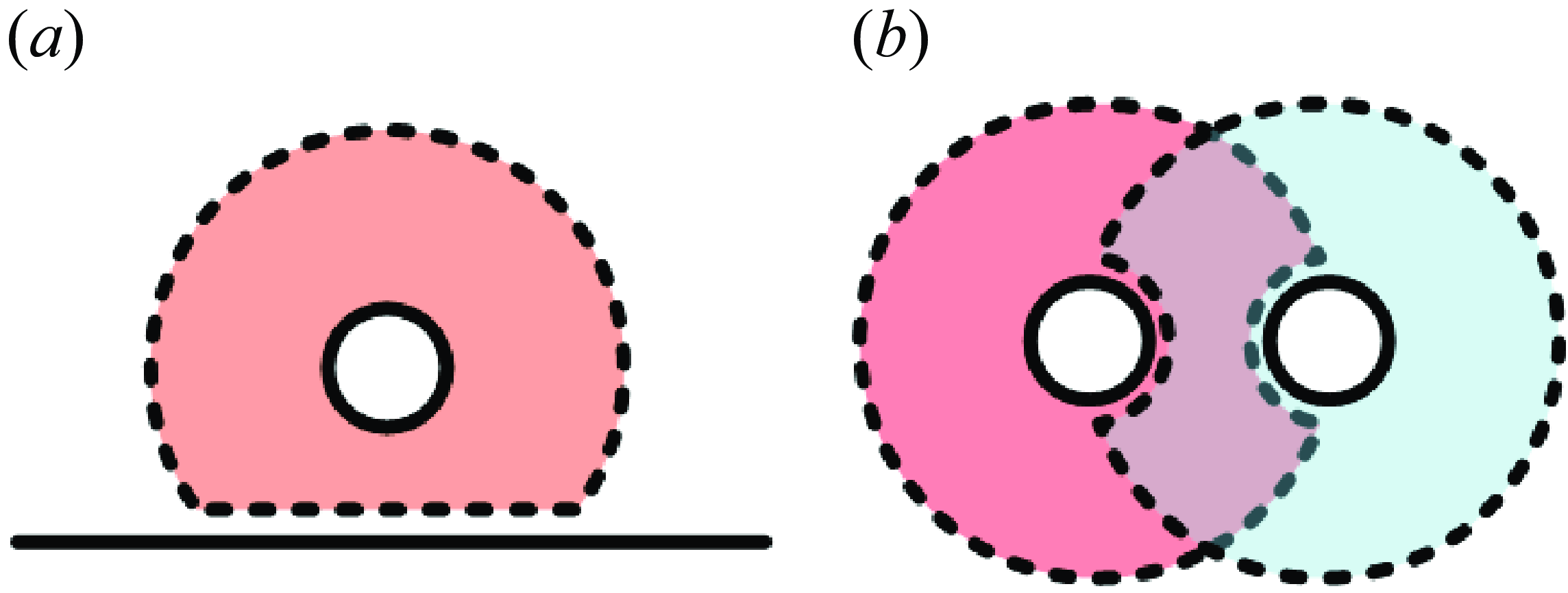
The particle interface boundaries may evolve due to particle movement, as shown in figure 4. When a particle is close to a global boundary, the particle subdomain is cut by the global boundary, and the interface boundary has a flat surface, as shown in figure 4(a). If two particles get close to each other, a small arched surface appears due to the presence of the adjacent particle, as shown in figure 4(b). Other special configurations can be considered as combinations of these two cases.
Schematics of interface boundaries due to particle movement. (a) A particle close to a global boundary. (b) Two particles close to each other. The solid lines represent global boundaries, and the dashed lines represent interface boundaries.

The fluid interface boundaries advance with the particle as well. In the Cartesian mesh, some mesh points are covered by the particle, as shown in figure 5(a). At these points, concentration is set as 0. As the particle moves, these mesh points may become uncovered, and solute concentrations should be evaluated at these points (see the red dots in figure 5 b). Similar situations happen to polar mesh points when the particle get close to fixed boundaries in the fluid subdomain. To update concentrations at these newly appeared points, we employ interpolations from other subdomains using (5.4) and (5.7) after advancing the particle.
Refilling of mesh points (red dots) at two consecutive time steps. The solid lines indicate the particle, and the dashed lines indicate the interface boundaries
 $ \Gamma _{fp}$
of the fluid subdomain
 $C_f$
.

Another problem arises when there are multiple particles. As two particles get too close to each other, there might not be enough Cartesian mesh points for interpolation using (5.7). At this time, the interface boundary conditions of one particle are interpolated from the subdomain of the other particle. This ensures accuracy without local mesh refinement.
6. Solution procedure
The full computational framework integrates the FBIM for fluid–structure interactions and the OMM for sharp-interface advection–diffusion problems. Given all values at time
 $t$
, the solutions at time
 $t + \Delta t$
are calculated by following procedures:
-
(i) Advance particles
 $\boldsymbol{X}(t + \Delta t)$
using (4.18).
-
(ii) Refill solute concentrations at newly appeared mesh points using (5.4) and (5.7).
-
(iii) Solve advection–diffusion problems (5.2) and (5.5) in each subdomain with global and interface boundary conditions, and update solute concentrations on particles
$c(\boldsymbol{X}, t + \Delta t)$
. -
(iv) Solve for surface force
$\boldsymbol{F}(\boldsymbol{X}, t + \Delta t)$
, desired velocity
$\boldsymbol{V}(\boldsymbol{X}, t + \Delta t)$
, translational velocity
$\boldsymbol{U}_{\!\!p}(\boldsymbol{X}, t + \Delta t)$
and rotational velocity
$\boldsymbol{ \Omega }_p(\boldsymbol{X}, t + \Delta t)$
using the pre-conditioner. -
(v) Solve the long range problem (3.5) with force density
$\boldsymbol{f}^l$
and the short range problem (3.6) using (3.24), and update flow field and velocities on boundaries (both particles and fixed boundaries).


The initial condition at
 $t = 0$
should be treated separately. When using zero fluid velocity and solute concentration (i.e.
 $\boldsymbol{u}(\boldsymbol{x}, 0) = \boldsymbol{0}$
and
 $c(\boldsymbol{x}, 0) = 0$
), the solution procedure starts from step (iii) for the first time step. If all variables are known at
 $t = 0$
, the simulation could start from step (i). If a non-zero solute concentration is known (
 $c(\boldsymbol{x}, 0) \neq 0$
) while other variables are unknown, an initialisation process is needed before starting the simulation. This is achieved in an iterative manner:
-
(i) Start with
$\boldsymbol{F}^0 = \boldsymbol{0}$
,
$\boldsymbol{u}^0 = \boldsymbol{0}$
and
$n = 0$
. -
(ii) Calculate
$\boldsymbol{U}_{\!\!p}^{n+1}$
,
$\boldsymbol{ \Omega }_p^{n+1}$
and
$\boldsymbol{F}^{n+1}$
with(6.1)
\begin{align}&\qquad\qquad \boldsymbol{U}_{\!\!p}^{n+1} = \begin{bmatrix} \text{Re}[\hat {u}_0^n] - M \text{Re}[\hat {c}_1] \\[5pt] \text{Im}[\hat {u}_0^n] + M \text{Im}[\hat {c}_1] \end{bmatrix},\\[-10pt]\nonumber \end{align}
(6.2)
\begin{align}&\qquad\qquad\qquad\quad \Omega _p^{n+1} = \text{Im}[\hat {u}_1^n],\\[-10pt]\nonumber \end{align}
(6.3)
\begin{align}& \hat {F}_k^{n+1} = \hat {F}_k^n + 4\hat {\alpha } |k| \left [M (1 - k) \hat {c}_{k-1} - \hat {u}_k^n\right ], k \neq 0, 1. \end{align}
-
(iii) Solve for fluid velocity
$\boldsymbol{u}^{n+1}$
using
$\boldsymbol{F}^{n+1}$
. -
(iv) Check if the residual of fluid velocity
$Res_{\boldsymbol{u}}$
is smaller than the pre-set tolerance, or the maximum iteration is reached. -
(v) Advance to the next iteration and jump to step (ii).
Here, the residual is defined as
(6.4)where
\begin{equation} Res_{\boldsymbol{u}} = max\left(\frac {||\boldsymbol{u}^{n+1} - \boldsymbol{u}^n||}{||\boldsymbol{u}^{n+1}||}\right), \end{equation}
$||\cdot ||$
is the L2-norm (
$||\boldsymbol{u}|| = \sqrt {\sum u_i^2}$
), and
$max$
function gives the maximum value over the computational domain. In practice, the tolerance of residual is set to be
$10^{-4}$
, and the maximum iteration number is 100.


7. Validations
In this section, the FBIM and the OMM are validated seperately by several numerical simulations. Their convergence behaviours are also presented. Here, we define the relative error of any parameter
 $*$
as
 \begin{equation} \varepsilon _{*} = \frac {|*_{(num)} - *_{(ref)}|}{|*_{(ref)}|}, \end{equation}
where
 $*_{(num)}$
and
 $*_{(ref)}$
are the numerical and reference solutions, respectively.
7.1. Parabolic flow with circular boundary
We first validate the FBIM by considering a simple parabolic flow, as shown in figure 6. The computational domain is a square of side length
 $L = 6.4$
. Periodic boundary conditions are employed in the
 $x$
and
 $y$
directions. A fixed circular boundary
 $ \Gamma$
of radius 2.5 is located at coordinates
 $(3.0, 3.0)$
, and the boundary condition reads
 \begin{equation} u_x|_{ \Gamma } = y^2, u_y|_{ \Gamma } = 0. \end{equation}
To enforce this boundary condition on
 $ \Gamma$
, a feedback force
 $\boldsymbol{F}$
is imposed by (4.2) with the desired velocity
 $\boldsymbol{V} = (y^2, 0)$
. With this boundary condition, a parabolic flow is created inside the area enclosed by
 $ \Gamma$
. The velocity due to this surface force is computed at coordinates
 $(3.2, 3.2)$
at
 $t = 20$
, and is used to measure the relative error. This set-up eliminates the effect of periodic boundary conditions, allowing comparison with analytical solution.
Schematic of the computational domain for parabolic flow with circular boundary.

Figure 7 shows the relative error of
 $u_x$
and the computational time by varying the number of mesh points
 $N_x$
and
 $N_y$
between 24 and 512. With fixed cutoff distance
 $r_c = L/16$
, we observe a fourth-order convergence, and the computational time per step scales as
 $1 / \Delta x$
. Here,
 $N = N_x \times N_y$
. When setting
 $r_c = 8\Delta x$
, the cutoff distance decreases linearly with the mesh size. On the one hand, decreasing
 $r_c$
leads to a lower-order convergence (first order); on the other hand, the computational time per step is hardly affected. This indicates that most of the computational time is spent on the short-range problem depending on
 $r_c$
. Taking both the accuracy and efficiency into consideration, the cutoff distance is set as
 $r_c = 8\Delta x$
in following simulations.
Validation and convergence study of the FBIM. (a) Convergence of velocity
 $u_x$
with respect to mesh size
 $\Delta x$
at coordinates
 $(3.2, 3.2)$
. (b) Computational time per step with respect to mesh size
 $\Delta x$
and number of Cartesian mesh points
 $N$
. Here,
 $N$
scales with
 $\Delta x^{-2}$
.

7.2. Initialisation for suspension of phoretic particles
In this subsection, the convergence of the pre-conditioner is validated. As shown in figure 8, the computational domain is a square of side length
 $L = 50$
, and periodic boundary conditions are applied in both directions. Ninety-five particles are randomly distributed in the fluid, and the area fraction is
 $\phi = 0.125$
. For each particle, an arbitrary but smooth solute concentration is given on its surface. The computational domain is discretised with a mesh size of
 $\Delta x = 1/15$
. The particle’s surface contains
 $N_e = 64$
evenly spaced elements. We choose 6 values of
 $\hat {\alpha }$
as 0.25, 0.5, 0.75, 1.0, 1.25 and 1.5. Simulations are performed for 100 iterations, following the initialisation process described in § 6.
Distribution of particles. Dashed lines represent periodic boundaries of the computational domain.

We first consider the case when
 $\hat {\alpha } = 1$
. The evolution of the residual
 $Res_{\boldsymbol{u}}$
is shown in figure 9(a). An exponential decay is observed with respect to iteration, and the tolerance
 $10^{-4}$
is reached within 17 iterations. We further pick a point
 $(-0.00170, 2.68629)$
which is located on the particle’s surface, and measure the surface force density at this point. To calculate the relative error of the surface force density
 $\varepsilon _{||\boldsymbol{F}||}$
, the surface force density at the 100th iteration is chosen as the reference solution. As shown in figure 9(b), an exponential convergence in the surface force density is observed with increasing iteration number. Moreover, the relative error
 $\varepsilon _{||\boldsymbol{F}||}$
is less than
 $1\, \%$
within 4 iterations.
Convergence of the pre-conditioner within 100 iterations. (a) Evolution of the residual
 $Res_{\boldsymbol{u}}$
with respect to iteration number. (b) Convergence of the surface force density
 $\boldsymbol{F}$
with respect to iteration number.

Then the effect of
 $\hat {\alpha }$
is analysed. For all cases except for
 $\hat {\alpha } = 1.5$
, the tolerance
 $10^{-4}$
is reached within 100 iterations (see figure 9
a). For
 $\hat {\alpha } \in [0.5, 1.0]$
, an error of
 $O(10^{-15})$
is obtained (see figure 9
b). However, the solution diverges when setting
 $\hat {\alpha } = 1.5$
. We also noticed that the convergence rate shows non-monotonic behaviour with respect to
 $\hat {\alpha }$
, as shown in figure 9. The fastest convergence is observed when
 $\hat {\alpha } = 1.0$
. Further increasing its value to 1.25 leads to a reduction of the convergence rate. Recall that, in § 4, we have mentioned that the value of
 $\hat {\alpha }$
should be less than 1 to avoid overshoot and divergence of solution. In the present case, there are no adjacent particles. Hence, setting
 $\hat {\alpha }$
around 1 could give good convergence. Besides, the presence of other fixed boundaries may contribute to the instability. Under this condition, decreasing the value of
 $\hat {\alpha }$
would help to stabilise the solution.
Schematic of the computational domain for single particle dynamics. The domain
 $C$
is decomposed into three overlapping subdomains: the fluid subdomain
 $C_f$
which coincides with
 $C$
, the particle subdomain
 $C_p$
and the outer subdomain
 $C_o$
. The solid lines represent the global boundaries, and the dashed lines represent the interface boundaries.

7.3. Single phoretic particle with finite system size
For the validation of the OMM, we consider a phoretic particle with limited system size. This problem has been studied analytically and numerically in Farutin et al. (Reference Farutin, Rizvi, Hu, Lin, Rafaï and Misbah2022). As shown in figure 10, the particle boundary
 $ \Gamma _p$
and the outer boundary
 $ \Gamma _o$
are concentric circles of radius 1 and
 $R = 3.25$
, respectively. Here,
 $R$
is the system size. The governing equations are (2.1) and (2.2) with 0 consumption/production rate (
 $\beta = 0$
). The boundary conditions are summarised as follows (Hu et al. Reference Hu, Lin, Rafai and Misbah2019):
 \begin{align}& \boldsymbol{u}(\boldsymbol{x}, t)|_{ \Gamma _p} = M \nabla _s c(\boldsymbol{x}, t)|_{ \Gamma _p} + \boldsymbol{U}_{\!\!p}(t) ,\end{align}
 \begin{align}& \boldsymbol{n} \boldsymbol{\cdot} \boldsymbol{\nabla} c(\boldsymbol{x}, t)|_{ \Gamma _p} = - A, c(\boldsymbol{x}, t)|_{ \Gamma _o} = 0. \end{align}
Moreover, the velocity attenuates to 0 in the far field. The flow field is calculated analytically by streamfunction (Sondak et al. Reference Sondak, Hawley, Heng, Vinsonhaler, Lauga and Thiffeault2016; Hu et al. Reference Hu, Lin, Rafai and Misbah2019). The solute concentration is computed by the OMM in a square domain
 $ \Omega$
. As shown in figure 10, the computational domain
 $ \Omega$
is decomposed into three overlapping subdomains. The fluid subdomain
 $ \Omega _f$
coincides with
 $ \Omega$
, and periodic boundary conditions are used in the
 $x$
and
 $y$
directions. The particle subdomain
 $ \Omega _p$
is an annular domain comoving with the particle (see the red ring in figure 10). Another annular subdomain (the outer subdomain
 $ \Omega _o$
, as shown by the blue ring in figure 10) is attached to the outer boundary
 $ \Gamma _o$
which also comoves with the particle. For the two annular subdomains, the global boundaries are represented by solid lines, and the boundary conditions follow (7.4), while the interface boundaries are labelled by dashed lines (see figure 10).
The particle velocity
 $||\boldsymbol{U}_{\!\!p}||$
and angular velocity
 $\omega _p$
obtained by the OMM are compared with the analytical results from Farutin et al. (Reference Farutin, Rizvi, Hu, Lin, Rafaï and Misbah2022), as shown in figure 11(a). Here, a non-zero angular velocity indicates circular motion. Good agreement between the two results is observed when setting the mesh size
 $\Delta x = 1/64$
. Convergence of the phoretic velocity
 $||\boldsymbol{U}_{\!\!p}||$
with respect to
 $\Delta x$
is demonstrated in figure 11(b), as the Péclet number is
 $Pe = 5.72$
. To calculate the relative error
 $\varepsilon _{||\boldsymbol{U}_{\!\!p}||}$
, the analytical result from Farutin et al. (Reference Farutin, Rizvi, Hu, Lin, Rafaï and Misbah2022) is used as a reference. As
 $\Delta x$
varies between
 $1/100$
to
 $1/32$
, a third-order accuracy is reached, thereby validating our implementation of the OMM.
Comparison between the analytical prediction and numerical simulation using the OMM. (a) Phoretic velocity
 $||\boldsymbol{U}_{\!\!p}||$
and angular velocity
 $\omega _p$
in stationary, straight and circular phases. The mesh size is
 $\Delta x = 1/64$
. (b) Convergence of phoretic velocity
 $||\boldsymbol{U}_{\!\!p}||$
with respect to mesh size
 $\Delta x$
at
 $Pe = 5.72$
. The system size is set to
 $R = 3.25$
. The analytical prediction is obtained by Farutin et al. (Reference Farutin, Rizvi, Hu, Lin, Rafaï and Misbah2022).

8. Applications
In this section, we combine the FBIM and the OMM to explore new simulations for single particle and many particles dynamics. First, we study particle swimming in a nearly infinite domain with periodic boundary conditions. Then self-propulsion of single particle in a straight channel is investigated, discovering an off-centred particle dynamics. We further show examples of particle suspensions in a square domain with periodic boundary conditions to reveal some interesting phenomena. Finally, particle pairing is studied by using quasistatic approximation.
8.1. Single particle in a nearly infinite domain
We first consider a similar case as presented in § 7.3, but with larger system size
 $R = 200$
, which is large enough to mimic an infinite domain (Hu et al. Reference Hu, Lin, Rafai and Misbah2019). The computational domain is a square and its size is
 $L = 409.6$
. The flow field is computed on a Cartesian mesh containing 8192 grid points in each direction, corresponding to a mesh size of
 $\Delta x = 0.05$
. The particle’s surface is discretised into
 $N_e = 128$
elements. The subdomain sizes are set as
 $r_p = 1.6$
for the two annular subdomains
 $ \Omega _p$
and
 $ \Omega _f$
. The radial and tangential meshes contain 32 and 128 grid points for
 $ \Omega _p$
, and 32 and 2560 grid points for
 $ \Omega _o$
, respectively.
Phoretic velocity
 $||\boldsymbol{U}_{\!\!p}||$
as a function of
 $Pe$
at
 $R = 200$
. The solid line represents the data obtained by Hu et al. (Reference Hu, Lin, Rafai and Misbah2019).

The phoretic velocity
 $||\boldsymbol{U}_{\!\!p}||$
computed by the FBIM-OMM is in good agreement with the published data (Hu et al. Reference Hu, Lin, Rafai and Misbah2019), as demonstrated in figure 12. We further plot particle trajectories for
 $Pe = 6, 12.8, 13$
in figure 13. At short enough time scale, the trajectories obtained by the FBIM-OMM are similar to those in Hu et al. (Reference Hu, Lin, Rafai and Misbah2019), as shown in the insets of figure 13. However, at larger time scales, the particle does not move along a straight line at
 $Pe = 6$
(figure 13
a), or along a circle at
 $Pe = 12.8$
(figure 13
b), as reported in Hu et al. (Reference Hu, Lin, Rafai and Misbah2019). Moreover, the chaotic motion at
 $Pe = 13$
is different from that in Hu et al. (Reference Hu, Lin, Rafai and Misbah2019) (see figure 13
c). These deviations result from the finite computational domain size
 $L$
and the periodic boundary conditions. In Hu et al. (Reference Hu, Lin, Rafai and Misbah2019), the flow velocity attenuates to 0 in the far field. In contrast, for the present work, the flow in the computational domain is affected by its images due to periodic boundary conditions. Although the domain size
 $L$
is 2 orders of magnitude larger than the particle radius, this effect is still non-negligible. For this reason, the particle trajectories are different in long scale.
Different trajectories obtained by the FBIM-OMM.

8.2. Single particle in a straight channel
In this subsection, we consider a phoretic particle immersed in a straight channel of length
 $L = 25.6$
and width
 $W = 5$
, as shown in figure 14. The computational domain is a rectangle of
 $25.6 \times 5.12$
, which is slightly wider than the channel. The two channel walls located at
 $y = 0$
and
 $y = 5$
. No-slip boundary conditions are imposed on these walls using the feedback force method, where the desired velocity is
 $\boldsymbol{V} = \boldsymbol{0}$
. The consumption rate is set to be
 $\beta = 0.01$
. Periodic boundary conditions are used at the left and right boundaries for both the flow and solute fields. At other boundaries, the boundary conditions follow (2.3) and (2.4). Other simulation parameters are: mesh size
 $\Delta x = 0.05$
, particle surface element number
 $N_e = 128$
and particle subdomain size
 $r_p = 0.8$
.
Steady-state relative solute concentration at
 $Pe = 2$
and 12, where the arrows indicate translational and rotational directions.

A transition from a stationary state to a centred straight state is found around
 $Pe_1 \approx 0.6$
, as shown in figure 15(a), which corresponds to a pitchfork bifurcation. In an unconfined geometry, the critical threshold
 $Pe_1$
can be obtained by following equation (Hu et al. Reference Hu, Lin, Rafai and Misbah2019):
 \begin{equation} Pe_1 = \frac {2(1 + R^2)}{\ln {R} + 1 + R^2 \ln {R} - R^2}. \end{equation}
Substituting
 $R = L/2 = 12.8$
into the equation above, we get
 $Pe_1 \approx 1.28$
for the unconfined case. This indicates that the presence of confinement leads to a reduction of the critical self-propulsion threshold (Picella & Michelin Reference Picella and Michelin2022). In the centred straight state (
 $0.6 \lesssim Pe \lesssim 8.0$
), the particle swims along the centre line of the channel, as shown in the top panel of figure 14. The evolution of
 $||\boldsymbol{U}_{\!\!p}||$
scales as
 $Pe^{-1/2}$
for the parameter range of the centred straight state except in the immediate vicinity of the threshold
 $Pe_1$
(see figure 15
b). Same behaviour has been reported by Picella & Michelin (Reference Picella and Michelin2022) for spherical particles in a cylindrical pipe.
Single particle swimming in a straight channel. (a) Phoretic velocity
 $||\boldsymbol{U}_{\!\!p}||$
, (b) same as (a) in logarithmic scale, (c) rotational velocity
 $||\boldsymbol{ \Omega }_p||$
and (d) lateral position
 $|y_p|$
at steady state.

A symmetry breaking is found around
 $Pe_2 \approx 8.0$
, so that the particle swims straightly at an off-centred position and rotates around its centre (see figure 15
c,d). Here,
 $y_p$
is the particle lateral position from the channel centre. According to our knowledge, this off-centred straight state has not been reported before. It should be noted that no external force is applied on the particle, which can push a particle towards a solid boundary (Desai & Michelin Reference Desai and Michelin2022). In the present case, the off-centred migration towards the channel wall emerges spontaneously as the particle becomes chemically more active (i.e.
 $Pe$
is increased). The particle rotation results from the hydrodynamic interaction between the particle and the solid boundary (Desai & Michelin Reference Desai and Michelin2022). When the particle is located in the centre of the channel, the hydrodynamic interactions of the two fixed boundaries are equal, and no rotational motion occurs. As the particle gets closer to one solid boundary than the other, it rotates clockwise (counter-clockwise) if the closest boundary is on the left (right) in the frame moving with the particle (see the white dashed arrow in the lower panel of figure 14).
8.3. Collective behaviours of particle suspension
In this subsection, we follow the study of Yang et al. (Reference Yang, Jiang, Picano and Zhu2024) and analyse collective behaviours of particle suspension. The computational domain is a square of side length
 $L = 50$
. The area fraction
 $\phi$
ranges from 0.05 to 0.2. The consumption rate is set to 0, so there is no consumption of solute. To avoid infinite growth of solute concentration, a constant value
 $c_0$
is subtracted from
 $c$
, when
 $min(c) \gt c_0$
. Periodic boundary conditions are applied in both directions. Other parameters are: mesh size
 $\Delta x = 1/15$
, particle surface element number
 $N_e = 64$
and particle subdomain size
 $r_p = 8/15$
.
The phase diagram is shown in figure 16. Quantitative agreement with Yang et al. (Reference Yang, Jiang, Picano and Zhu2024) is observed for most cases, as our results reproduce the crystalline solid (hexagon), liquid(star) and dynamic chaining (diamond). The solid curve is fitted with
 $\phi ^{1/2}$
, indicating the theoretical prediction of the solid–liquid transition given by Yang et al. (Reference Yang, Jiang, Picano and Zhu2024). Discrepancy is found at
 $(Pe, \phi ) = (3.5, 0.2)$
, where we obtain liquid, while Yang et al. (Reference Yang, Jiang, Picano and Zhu2024) reported dynamic chaining. As stated in the introduction, Yang et al. (Reference Yang, Jiang, Picano and Zhu2024) used an immersed-boundary-based method, which would slightly overestimate the phoretic velocity. For this reason, it is reasonable that dynamic chaining which requires larger phoretic velocity is observed at lower
 $Pe$
in their work. Moreover, Yang et al. (Reference Yang, Jiang, Picano and Zhu2024) have pointed out that, with large enough domains (their domain is twice ours), particles would be more likely to form patterns like dynamic chaining and active turbulence. This could be a potential source to explain the minor discrepancy observed here. The effect of domain size on suspension of particles would be an interesting topic, which requires systematic studies in the future.
Phase diagram over the area fraction
 $\phi$
and the Péclet
 $Pe$
: crystalline solid (blue hexagon), liquid (orange star) and dynamic chaining (green diamond). The solid line scales as
 $\phi ^{1/2}$
, indicating the theoretical prediction of the solid–liquid transition in Yang et al. (Reference Yang, Jiang, Picano and Zhu2024).

We further analyse the solid–liquid transition at
 $\phi = 0.05$
. When
 $Pe \lesssim 1.5$
, the particles self-organise into a hexagonal solid, as shown in figure 17(a). A novel phase emerges around
 $Pe \approx 1.6$
. As shown in figure 17(b), each particle vibrates periodically around an equilibrium position, resembling a crystal lattice vibration (see the supplementary movie). As far as our knowledge goes, this lattice vibration state of phoretic particle suspension is observed for the first time. By slightly increasing
 $Pe$
to 1.7, the particles become more active, mimicking the behaviour of liquid molecules.
Snapshots of particles and relative solute concentration at (a)
 $Pe = 1.5$
and (b)
 $Pe = 1.6$
. The arrows indicate instantaneous translational directions.

8.4. Quasistatic approximation of particle pairs
In order to investigate the behaviour of near-contact particles, we perform a quasistatic approximation of two particles in this subsection. The idea is to fix the particle centres, let them relax to a steady state and then measure their velocities. The computational domain is a square of side length
 $L = 100$
with periodic boundary conditions applied in both directions. Two particles are placed in the domain with an inter-particle distance
 $d_{12}$
, as shown in figure 18(a). The consumption rate is set to 0, and a constant value
 $c_0$
is subtracted from the concentration field, as described in previous subsection. Other parameters are: mesh size
 $\Delta x = 0.05$
, particle surface element number
 $N_e = 128$
and particle subdomain size
 $r_p = 0.8$
.
Quasistatic approximation of particle pairs at
 $Pe = 1$
. (a) Particle velocities
 $U_x$
versus inter-particle distance
 $d_{12}$
. The blue line and markers correspond to particle 1 and the orange ones to particle 2. The inset is the schematic of the particle pair. (b) Convergence of velocity
 $|U_x|$
with respect to mesh size
 $\Delta x$
at
 $d_{12} = 0.3$
.

First, we fix the Péclet number as
 $Pe = 1$
and consider the effect of inter-particle distance
 $d_{12}$
. At this Péclet number, the two particles tend to repel each other, so their velocities
 $U_x$
have the same magnitude but opposite directions, as shown in figure 18(a). As
 $d_{12}$
is increased, the hydro-chemical interaction between the two particles is reduced, hence the magnitude of
 $U_x$
is decreased. This is confirmed by using different
 $\Delta x$
(
 $N_e$
scales as
 $1/\Delta x$
) as shown in figure 18(a). We further perform convergence study at
 $d_{12} = 0.3$
. The result at
 $\Delta x = 1/60$
is used as a reference to calculate the relative error
 $\varepsilon _{|U_x|}$
. As shown in figure 18(b), a second-order accuracy is reached for the present case.
Quasistatic approximation of particle pairs at
 $d_{12} = 0.3$
. (a,b) Snapshots of particles and relative solute concentration. The arrows indicate translational and rotational directions. (c) Particle velocity
 $|U_x|$
and (d) rotational velocity
 $||\boldsymbol{ \Omega }||$
versus Péclet number
 $Pe$
.

Then the effect of Péclet number
 $Pe$
is studied when the inter-particle distance is fixed at
 $d_{12} = 0.3$
. When
 $Pe \lesssim 2.0$
, the two particles tend to swim straightly in opposite directions. The concentration field is symmetric along the
 $x$
axis as shown in figure 19(a). By increasing the Péclet number, this up-and-down symmetry breaks down, leading to non-zero velocity in the
 $y$
direction and rotation, as shown in figure 19(b). In the far field, the two particles as a whole can be seen as a pusher-like swimmer. For
 $Pe \gtrsim 5.0$
, the translational velocity
 $|U_i|$
scales as
 $Pe^{-1}$
and the rotational velocity
 $||\boldsymbol{ \Omega }||$
scales as
 $Pe^{-0.4}$
, as depicted in figure 19(c,d). The decrease of
 $|U_x|$
with
 $Pe$
indicates that the two particles might form stable or dynamic pair at high enough
 $Pe$
.
9. Conclusion
In this work, we present a full numerical framework for phoretic particles that allows us to efficiently simulate the multiparticle dynamics in periodic or confined geometries. This framework consists of a FBIM for fluid–structure interactions in Stokes flow, and an OMM for advection–diffusion problems with moving boundaries. The FBIM decomposes the Stokes equations into short-range and long-range parts, so that the former is computed by boundary integral equation within a cutoff distance, while the latter is solved by a Fourier spectral method accelerated by FFT. To resolve moving boundaries in advection–diffusion problems, the OMM divides the computational domain into several overlapping subdomains, which are allowed to move independently. The FBIM and the OMM are then validated separately, showing relatively high-order accuracy. We further apply this framework to more general problems, including a single particle in a nearly infinite domain, a single particle in a straight channel, collective behaviours of particle suspensions and a quasistatic approximation of particle pairs. Quantitative agreements with published results are observed, further verifying the proposed framework. Moreover, novel phenomena are reported such as off-centred motion in a straight channel, the lattice vibration phase of particle suspensions and particle pairing at high Péclet number, which are worth systematic studies in the future. This framework can be further extended to non-circular rigid particles (Zhu & Zhu Reference Zhu and Zhu2023) and even deformable particles, which will be our future research. With slight modification, it can be used to simulate a variety of active objects which interact/communicate through solute concentration, such as Janus particles and quorum sensing of bacteria (Ziepke et al. Reference Ziepke, Maryshev, Aranson and Frey2022). Hence, this framework could contribute to theoretical and numerical studies of active matter in a quite broad context.
Supplementary movie
Supplementary movie is available at https://doi.org/10.1017/jfm.2025.10282.
Acknowledgements
All the computations presented in this paper were performed using the GRICAD infrastructure (https://gricad.univ-grenoble-alpes.fr), which is supported by Grenoble research communities, and using computing resources at the High Performance Computing Center of Central South University.
Funding
This work was supported by National Natural Science Foundation of China (No. 52175263), CNES (Centre National d’Etudes Spatiales) and the French-German university program “Living Fluids” (Grant CDFA-Q1-14).
Declaration of interests
The authors report no conflict of interest.
Appendix A. Long-range density
A natural choice of
 $D^l(r)$
is the polynomial, of which the high-order derivatives are continuous. In practice, we chose a sixth-order polynomial
 $D^l(r) = \sum _{i = 0}^6 a_i r^i$
and set
 \begin{equation} \left . \frac {\partial ^k D^l}{\partial r^k} \right |_{r = r_c} = 0, \left . \frac {\partial D^l}{\partial r} \right |_{r = 0} = 0, \end{equation}
where
 $k = 0, 1, 2, 3$
.
The integral in (3.10) can be written in polar coordinates, and the following equation is obtained as:
 \begin{equation} G_{ij}(\boldsymbol{x}, \boldsymbol{x}^v) = \int _0^{r_c} D^l(r') r' \left [ \int _{0}^{2\pi } G_{ij}(\boldsymbol{r}, \boldsymbol{r}') {\rm d}\theta \right ] {\rm d}r', \end{equation}
where
 $\boldsymbol{r}' = \boldsymbol{x}' - \boldsymbol{x}^v$
and
 $\theta$
is the angle between
 $\boldsymbol{r}$
and
 $\boldsymbol{r}'$
. Substituting (3.2) into the equation above and integrating over
 $\theta$
, we obtain the following equation:
 \begin{equation} G_{ij}(\boldsymbol{x}, \boldsymbol{x}^v) = 2\pi G_{ij}(\boldsymbol{x}, \boldsymbol{x}^v) \int _0^{r_c} D^l(r') r' {\rm d}r' + \pi \frac {r_i^* r_j^* - r_i r_j}{r^4} \int _0^{r_c} D^l(r') r'^3 {\rm d}r'. \end{equation}
Here,
 $\boldsymbol{r}^*$
is the vector perpendicular to
 $\boldsymbol{r}$
. To satisfy (A3), we set
 \begin{equation} \int _0^{r_c} D^l(r') r' {\rm d}r' = \frac {1}{2\pi }, \int _0^{r_c} D^l(r') r'^3 {\rm d}r' = 0. \end{equation}
By solving the system of (A1) and (A4), we obtain the polynomial coefficients, and the long-range density is given as
 \begin{align} &D^l(r) =\nonumber\\& \left \{ \begin{aligned} &0, & r \geqslant r_c \\ &\frac {56}{3 \pi r_c^2} \left [-\frac {25}{2}\left(\!\frac {r}{r_c}\!\right)^6 + 54\left(\!\frac {r}{r_c}\!\right)^5 - 90\left(\!\frac {r}{r_c}\!\right)^4 + 70\left(\!\frac {r}{r_c}\!\right)^3 - \frac {45}{2}\left(\!\frac {r}{r_c}\!\right)^2 + 1 \right ], & r \lt r_c \end{aligned} \right . . \end{align}
Appendix B. Short-range Green’s function
Rewriting the integral in (3.16) in polar coordinate and substituting (3.11) and (3.15), the short-range boundary integral equation becomes
 \begin{equation} \begin{aligned} u_i^s(\boldsymbol{x}) &= \frac {1}{4 \pi } g_j^v G_{ij}(\boldsymbol{x}, \boldsymbol{x}^v) - \frac {1}{4 \pi } g_j^v \int _0^{r_c} D^l(r') r' \left [ \int _{0}^{2\pi } G_{ij}(\boldsymbol{r}, \boldsymbol{r}') {\rm d}\theta \right ] {\rm d}r' \\ &= \frac {1}{4 \pi } g_j^v G_{ij}(\boldsymbol{x}, \boldsymbol{x}^v) - A_1 g_j^v G_{ij}(\boldsymbol{x}, \boldsymbol{x}^v) - A_2 g_j^v (r_i^* r_j^* - r_i r_j) - A_3 g_j^v \delta _{ij}\! - A_4 g_j^v \delta _{ij}, \end{aligned} \end{equation}
where
 \begin{equation} \begin{aligned} A_1 &= \tfrac {1}{2} \int _0^r D^l(r') r' {\rm d}r' \\ &= \frac {28}{3 \pi } \left [ - \frac {25}{16} \left(\frac {r}{r_c}\right)^8 \!{+}\, \frac {54}{7} \left(\frac {r}{r_c}\right)^7 \!{-}\, 15 \left(\frac {r}{r_c}\right)^6 \! {+} \,14 \left(\frac {r}{r_c}\right)^5 \!{-}\, \frac {45}{8} \left(\frac {r}{r_c}\right)^4 \!{+} \,\frac {1}{2} \left(\frac {r}{r_c}\right)^2 \right ], \\ A_2 &= \frac {1}{4 r^4} \int _0^r D^l(r') r'^3 {\rm d}r' \\ &= \frac {14}{3 \pi r_c^2} \left [ - \frac {5}{4} \left(\frac {r}{r_c}\right)^6 + 6 \left(\frac {r}{r_c}\right)^5 - \frac {45}{4} \left(\frac {r}{r_c}\right)^4 + 10 \left(\frac {r}{r_c}\right)^3 - \frac {15}{4} \left(\frac {r}{r_c}\right)^2 + \frac {1}{4} \right ], \\ A_3 &= - \tfrac {1}{2} \int _r^{r_c} D^l(r') r' \ln (r') {\rm d}r'\\ &= - \frac {28}{3 \pi } \left [ - \frac {25}{128} \left(\frac {r}{r_c}\right)^8 + \frac {54}{49} \left(\frac {r}{r_c}\right)^7 - \frac {5}{2} \left(\frac {r}{r_c}\right)^6 + \frac {14}{5} \left(\frac {r}{r_c}\right)^5 - \frac {45}{32} \left(\frac {r}{r_c}\right)^4 \right . \\ &\quad + \frac {1}{4} \left(\frac {r}{r_c}\right)^2 - \frac {1583}{31360} + \frac {25}{16} \left(\frac {r}{r_c}\right)^8 \ln (r) - \frac {54}{7} \left(\frac {r}{r_c}\right)^7 \ln (r) + 15 \left(\frac {r}{r_c}\right)^6 \ln (r) \\ &\quad - 14 \left(\frac {r}{r_c}\right)^5 \ln (r) + \frac {45}{8} \left(\frac {r}{r_c}\right)^4 \ln (r) \left . - \frac {1}{2} \left(\frac {r}{r_c}\right)^2 \ln (r) + \frac {3}{112} \ln \left(r_c\right) \right ],\\ A_4 &= \tfrac {1}{4} \int _r^{r_c} D^l(r') r' {\rm d}r'\\ &= \frac {14}{3 \pi } \left [ \frac {25}{16} \left(\frac {r}{r_c}\right)^8 - \frac {54}{7} \left(\frac {r}{r_c}\right)^7 + 15 \left(\frac {r}{r_c}\right)^6 - 14 \left(\frac {r}{r_c}\right)^5 + \frac {45}{8} \left(\frac {r}{r_c}\right)^4 - \frac {1}{2} \left(\frac {r}{r_c}\right)^2\right . \\ &\quad + \left .\frac {3}{112} \right ]. \end{aligned} \end{equation}
Then the short-range Green’s function is obtained as
 \begin{equation} \begin{aligned} G_{ij}^s (\boldsymbol{x}, \boldsymbol{x}^v) &= \int _{ \Omega _c} G_{ij}(\boldsymbol{x}, \boldsymbol{x}') D^s(|\boldsymbol{x}' - \boldsymbol{x}^v|) {\rm d}\boldsymbol{x}'\\ &= (1 - 4 \pi A_1) G_{ij} (\boldsymbol{x}, \boldsymbol{x}^v) - 4 \pi A_2 (r_i^* r_j^* - r_i r_j) - 4 \pi (A_3 + A_4) \delta _{ij}. \end{aligned} \end{equation}
Appendix C. Translational and rotational velocities for freely moving phoretic particles
Substituting (4.2) into (4.4), one obtains
 \begin{equation} \begin{aligned} \int _{ \Gamma _p} \boldsymbol{F}(\boldsymbol{X}, t) {\rm d}S(\boldsymbol{X}) &+ \int _{ \Gamma _p} \alpha \left [ \boldsymbol{V}(\boldsymbol{X}, t + \Delta t) - \boldsymbol{u}(\boldsymbol{X}, t) \right ] \Delta t {\rm d}S(\boldsymbol{X}) = \boldsymbol{0},\\ \int _{ \Gamma _p} (\boldsymbol{X} - \boldsymbol{X}_{\!p}) \times \boldsymbol{F}(\boldsymbol{X}, t) {\rm d}S(\boldsymbol{X}) &+ \int _{ \Gamma _p} (\boldsymbol{X} - \boldsymbol{X}_{\!p}) \\&\quad \times \alpha \left [ \boldsymbol{V}(\boldsymbol{X}, t + \Delta t) - \boldsymbol{u}(\boldsymbol{X}, t) \right ] \Delta t {\rm d}S(\boldsymbol{X}) = \boldsymbol{0}. \end{aligned} \end{equation}
The first terms on the left side of (C1) vanish. As
 $\alpha$
and
 $\Delta t$
are non-zero constants, (C1) can be simplified as
 \begin{align} &\int _{ \Gamma _p} \left [ \boldsymbol{V}(\boldsymbol{X}, t + \Delta t) - \boldsymbol{u}(\boldsymbol{X}, t) \right ] {\rm d}S(\boldsymbol{X}) = \boldsymbol{0},\nonumber\\& \int _{ \Gamma _p} (\boldsymbol{X} - \boldsymbol{X}_{\!p}) \times \left [ \boldsymbol{V}(\boldsymbol{X}, t + \Delta t) - \boldsymbol{u}(\boldsymbol{X}, t) \right ] {\rm d}S(\boldsymbol{X}) = \boldsymbol{0}. \end{align}
Here,
 $\boldsymbol{U}_{\!\!p}(t + \Delta t)$
and
 $\boldsymbol{ \Omega }_p(t + \Delta t)$
can be solved for by substituting (4.3) into the above equation as
 \begin{align} \boldsymbol{ \Omega }_p(t + \Delta t) &= \frac {\int _{ \Gamma _p} (\boldsymbol{X} - \boldsymbol{X}_{\!p}) {\rm d}S(\boldsymbol{X}) \times \int _{ \Gamma _p} \tilde {\boldsymbol{u}}(\boldsymbol{X}, t + \Delta t) {\rm d}S(\boldsymbol{X})}{P \int _{ \Gamma _p} (\boldsymbol{X} - \boldsymbol{X}_{\!p})^2 {\rm d}S(\boldsymbol{X}) - \left [ \int _{ \Gamma _p} (\boldsymbol{X} - \boldsymbol{X}_{\!p}) {\rm d}S(\boldsymbol{X}) \right ]^2} \nonumber\\[5pt] &\quad - \frac {P \int _{ \Gamma _p} (\boldsymbol{X} - \boldsymbol{X}_{\!p}) \times \tilde {\boldsymbol{u}}(\boldsymbol{X}, t + \Delta t) {\rm d}S(\boldsymbol{X})}{P \int _{ \Gamma _p} (\boldsymbol{X} - \boldsymbol{X}_{\!p})^2 {\rm d}S(\boldsymbol{X}) - \left [ \int _{ \Gamma _p} (\boldsymbol{X} - \boldsymbol{X}_{\!p}) {\rm d}S(\boldsymbol{X}) \right ]^2}, \end{align}
 \begin{equation} \boldsymbol{U}_{\!\!p}(t + \Delta t) = \frac {\boldsymbol{ \Omega }_p(t + \Delta t) \times \int _{ \Gamma _p} (\boldsymbol{X} - \boldsymbol{X}_{\!p}) {\rm d}S(\boldsymbol{X}) - \int _{ \Gamma _p} \tilde {\boldsymbol{u}}(\boldsymbol{X}, t + \Delta t) {\rm d}S(\boldsymbol{X})}{P}, \end{equation}
where
 $P = \int _{ \Gamma _p} {\rm d}S(\boldsymbol{X})$
is the perimeter of particle, and
 $\tilde {\boldsymbol{u}}(\boldsymbol{X}, t + \Delta t) = M \nabla _s c(\boldsymbol{X}, t + \Delta t) - \boldsymbol{u}(\boldsymbol{X}, t)$
. Specifically, for circular particles,
 \begin{align} \int _{ \Gamma _p} (\boldsymbol{X} - \boldsymbol{X}_{\!p}) {\rm d}S(\boldsymbol{X}) = \boldsymbol{0},\nonumber\\ \int _{ \Gamma _p} (\boldsymbol{X} - \boldsymbol{X}_{\!p}) \times M \nabla _s c(\boldsymbol{X}) {\rm d}S(\boldsymbol{X}) = \boldsymbol{0},\nonumber\\ \int _{ \Gamma _p} (\boldsymbol{X} - \boldsymbol{X}_{\!p})^2 {\rm d}S(\boldsymbol{X}) = 2\pi a^3,\nonumber\\ P = \int _{ \Gamma _p} {\rm d}S(\boldsymbol{X}) = 2\pi a, \end{align}
where
 $a$
is the particle radius. Then
 $\boldsymbol{U}_{\!\!p}$
and
 $\boldsymbol{ \Omega }_p$
can be simplified to
 \begin{align}& \boldsymbol{U}_{\!\!p}(t + \Delta t) = \frac {1}{2 \pi a} \int _{ \Gamma _p} \left [ \boldsymbol{u}(\boldsymbol{X}, t) - M \nabla _s c(\boldsymbol{X}, t + \Delta t) \right ] {\rm d}S(\boldsymbol{X}),\\[-10pt]\nonumber \end{align}
 \begin{align}&\qquad \boldsymbol{ \Omega }_p(t + \Delta t) = \frac {1}{2 \pi a^3} \int _{ \Gamma _p} (\boldsymbol{X} - \boldsymbol{X}_{\!p}) \times \boldsymbol{u}(\boldsymbol{X}, t) {\rm d}S(\boldsymbol{X}). \end{align}
It should be noted that the surface velocity
 $\boldsymbol{u}(\boldsymbol{X}, t)$
of a particle (the
 $m$
th boundary in the fluid domain) is induced by two parts: the surface force density of the particle itself, and the surface force density of other particles and fixed boundaries, as
 \begin{align} \boldsymbol{u}(\boldsymbol{X}, t)|_{ \Gamma _p} &= \frac {1}{4\pi } \int _{ \Gamma _p} \boldsymbol{G}(\boldsymbol{X}, \boldsymbol{X}') \boldsymbol{F}(\boldsymbol{X}', t) {\rm d}S(\boldsymbol{X}') + \frac {1}{4\pi } \sum _{n \neq m} \int _{ \Gamma _n} \boldsymbol{G}(\boldsymbol{X}, \boldsymbol{X}') \boldsymbol{F}(\boldsymbol{X}', t) {\rm d}S(\boldsymbol{X}') \nonumber\\ &= \boldsymbol{u}_p(\boldsymbol{X}, t) + \boldsymbol{u}_{rest}(\boldsymbol{X}, t). \end{align}
Here,
 $\boldsymbol{u}_p$
and
 $\boldsymbol{u}_{rest}$
are the surface velocity induced by the particle itself and by other particles and fixed boundaries, respectively.
When there is only one circular particle in an unbounded fluid,
 $\boldsymbol{u}_{rest}$
vanishes. Using the force-free and torque-free conditions on the circular particle, one can show that
 $\boldsymbol{u}_p$
always satisfies
 \begin{equation} \int _{ \Gamma _p} \boldsymbol{u}_p(\boldsymbol{X}, t) {\rm d}S(\boldsymbol{X}) = \boldsymbol{0}, \int _{ \Gamma _p} (\boldsymbol{X} - \boldsymbol{X}_{p}) \times \boldsymbol{u}_p(\boldsymbol{X}, t) {\rm d}S(\boldsymbol{X}) = \boldsymbol{0}. \end{equation}
 \begin{align}& \boldsymbol{U}_{p}(t + \Delta t) = - \frac {1}{2 \pi a} \int _{ \Gamma _p} M \nabla _s c(\boldsymbol{X}, t + \Delta t) {\rm d}S(\boldsymbol{X}), \end{align}
 \begin{align}&\qquad\qquad\qquad\qquad \boldsymbol{ \Omega }_{p}(t + \Delta t) = \boldsymbol{0}, \end{align}
in agreement with those obtained by the reciprocal theorem (Hu et al. Reference Hu, Lin, Rafai and Misbah2019).
When there are other particles and fixed boundaries,
 $\boldsymbol{u}_{rest}$
enters (C6) and (C7), resulting in non-zero contribution to the translational and rotational velocities.
Since
 $\boldsymbol F$
at the
 $n$
th boundary contains contributions from
 $\boldsymbol u$
at the same
 $n$
th boundary at previous iterations, according to the feedback force procedure ((4.2) or (4.14))
 \begin{equation} \boldsymbol{F}(\boldsymbol{X}, t)|_{ \Gamma _n} = \boldsymbol{F}(\boldsymbol{X}, t - \Delta t)|_{ \Gamma _n} + \alpha \left [ \boldsymbol{V}(\boldsymbol{X}, t)|_{ \Gamma _n} - \boldsymbol{u}(\boldsymbol{X}, t - \Delta t)|_{ \Gamma _n} \right ] \Delta t, \end{equation}
which, in turn, contains contributions from
 $\boldsymbol F$
at the
 $m$
th boundary (which is the particle
 $ \Gamma _p$
) according to the boundary integral equation
 \begin{equation} \begin{aligned} \boldsymbol{u}(\boldsymbol{X}, t - \Delta t)|_{ \Gamma _n} &= \frac {1}{4\pi } \int _{ \Gamma _n} \boldsymbol{G}(\boldsymbol{X}, \boldsymbol{X}') \boldsymbol{F}(\boldsymbol{X}', t - \Delta t) {\rm d}S(\boldsymbol{X}') \\ &\quad + \frac {1}{4\pi } \int _{ \Gamma _p} \boldsymbol{G}(\boldsymbol{X}, \boldsymbol{X}') \boldsymbol{F}(\boldsymbol{X}', t - \Delta t) {\rm d}S(\boldsymbol{X}') \\ &\quad + \frac {1}{4\pi } \sum _{l \neq m, n} \int _{ \Gamma _l} \boldsymbol{G}(\boldsymbol{X}, \boldsymbol{X}') \boldsymbol{F}(\boldsymbol{X}', t - \Delta t) {\rm d}S(\boldsymbol{X}'), \end{aligned} \end{equation}
 \begin{align} \boldsymbol{F}(\boldsymbol{X}, t - \Delta t)|_{ \Gamma _p} = \boldsymbol{F}(\boldsymbol{X}, t - 2\Delta t)|_{ \Gamma _p} + \alpha \left [ \boldsymbol{V}(\boldsymbol{X}, t - \Delta t)|_{ \Gamma _p} - \boldsymbol{u}(\boldsymbol{X}, t - 2\Delta t)|_{ \Gamma _p} \right ] \Delta t,\nonumber\\[3pt] \end{align}
where
 $\boldsymbol{u}_{rest}$
contains a non-trivial contribution of
 $\nabla _s c$
at that particle (the
 $m$
th boundary), recalling that
 $\boldsymbol{V}$
contains
 $M \nabla _s c$
for phoretic particles. This shows how the iterative procedure is capable of capturing the non-scalar relation between the slip velocity
 $M \nabla _s c$
at the boundary of a circular particle and the swimming velocity
 $\boldsymbol{U}_{\!\!p}$
and
 $\boldsymbol{ \Omega }_p$
of the same particle in a complex geometry defined by rigid boundaries and other particles, despite using the simple expressions (C6) and (C7) at each iteration.
For arbitrarily shaped particles, (C9) no longer holds, so that both
 $\boldsymbol{u}_p$
and
 $\boldsymbol{u}_{rest}$
also contribute to
 $\boldsymbol{U}_{\!\!p}$
and
 $\boldsymbol{ \Omega }_p$
. As
 $\boldsymbol{u}_p$
and
 $\boldsymbol{u}_{rest}$
are the convolution of the Green’s function
 $\boldsymbol{G}$
and the surface force density
 $\boldsymbol{F}$
(see (C8)), this results in an anisotropic (tensorial) relation between
 $\boldsymbol{U}_{\!\!p}$
,
 $\boldsymbol{ \Omega }_p$
and
 $\nabla _s c$
.