1.0 Introduction
The aerodynamic industry, and the field of aerodynamic design, is one of the most challenging and difficult industries today due to its complexity in the different factors involved as well as their interactions. As there are many different design factors and their interactions with the real world to consider, simulation-based design methods of aerodynamic design involve complex modelling and simulations to test and validate solutions [Reference Jameson1]. The simulation-based design method also has the benefit of being able to test solutions and variations without massive capital investment involved with physically building an aircraft. However, simulation-based design also has the downside of being computationally expensive and time-consuming, requiring a large capital investment in terms of computing hardware [Reference Jameson2].
One of the newer methods of approaching this problem of designing and testing different solutions involve the principle of optimisation – more specifically, algorithm-based optimisation. Algorithm-based optimisation is a mathematics-based method of finding optimal operating conditions and trade-off relationships between different factors of interest. With the rapid development in computing capacity and software design, optimisation methods, such as multi-objective optimisation, have grown as an effective way of analysing the complex relationships between different factors, and are being used more widely across different fields of engineering [Reference Marler and Arora3], including various optimal aeronautical structure design cases [Reference Chen, Wang, Sun and Bai4–Reference Dati, De Angelis, Marrone, Lampani, Gaudenzi and Bernabei7], providing insights or possibilities that have not previously been consideredbefore.
However, not all parts of the aerodynamic industry employ such methodology in their operations. Manufacturing in the aero-industry is one such field, where the manufacturers of various parts of the aircraft are mainly dependent on the designers of the parts to produce the specifications, without much regard to their ease of manufacturing. This stems mainly from the high-risk nature of the industry itself, where the monetary importance of being able to produce a part at a slightly cheaper price is much less significant compared to the safety-critical importance of producing a part which is exactly compliant with the design specifications. Recently, the trend in aerospace industry is becoming more and more focused towards faster production and rapid development cycles, with division of demand based on customers’ specific needs [Reference Maginness, Shehab, Beadle and Carswell8, Reference Rebentisch, Myles Murman and Earll9], which also puts more pressure on the manufacturers in meeting the various needs within time. While such trends have led to more interest in the implementation of lean manufacturing [Reference Nikhil Bharadwaj, Shiva Shashank, Harish and Garre10], there is still significant room for improvement in the design and manufacturing of aerospace parts [Reference Crute, Ward, Brown and Graves11], as there has been little opportunity to optimise the design of a part with its manufacturing characteristics in mind.
Due to this disparity between the design and manufacturing of parts, an optimisation model which takes not only aerodynamic but also manufacturing characteristics in the design of a part was deemed necessary. For this purpose, a Python-based machine-learning model was created using the combined data between aerodynamic and manufacturing data of an aircraft rib. This model was then presented to a multi-objective optimisation algorithm to explore different options within the provided limits obtained from the machine learning models, to explore the impact on the design of parts induced by the inclusion of their corresponding manufacturing characteristics.
This study is composed of two main studies exploring two different aspects of optimisation with both design and manufacturing characteristics.
The first study involves building of a machine learning model that can accurately predict the behaviour of the rib based on the combined data between aerodynamic performance and manufacturing efficiency, then performing multi-objective optimisation to understand the trade-off relationship between manufacturing and design characteristics.
The second study explores the impact in aerodynamic performance due to the inclusion of manufacturing characteristics by introducing new variables, the front and rear spar positions. The extended dataset including values from the new variables was used to build a machine learning model and perform multi-objective optimisation, same as the first study. The results of the optimisations from the first and second study were compared to analyse the change in the optimal trade-off points due to the inclusion of spar positions.
2.0 Problem identification
The main identified problem, as briefly mentioned in the Introduction, was the lack of sufficient back-and-forth communication between design and manufacturing. The aircraft rib design is generated according to the desired aerofoil shape by the designer of the aircraft, then the shape of the rib is communicated to the manufacturer of the rib for production. During this process, there is little input from the manufacturer on what the rib shape should look like, as the requirements of the shape depend on the aerodynamic performance of the rib, which is decided by the designer of the wing.
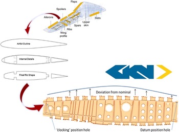
This means the manufacturer has little opportunity to express its opinion on what type of design is most desirable for the efficiency of its manufacturing process. The manufacturer tries to meet the specifications given to it as closely as possible, but depending on what kind of manufacturing processes or tools are available to the manufacturer, the final manufactured rib may deviate from the initial intended design (see Fig. 1). Also, the manufacturer’s choice in which process and tools to use depends largely on the given specification, rather than what is efficient for the manufacturer, so its efficiency in processes and manufacturing is less than optimal.
The design and manufacturing process of an aircraft rib.

This means there is potential for improvement in both the performance of the rib and its manufacturing efficiency. Currently, the two main objectives in manufacturing a rib – aerodynamic performance and manufacturing efficiency – are considered separately. However, there is a great potential benefit in being able to consider both sides of the issue at once, and finding conditions that satisfy both sides the most at the same time. By considering the relevant manufacturing characteristics in the design stage of the rib, the relationships and trade-offs between better-performing design and their manufacturing challenges can be understood better, and optimal operating conditions can be found.
Furthermore, exploring multiple objectives at the same time can open more opportunities for improvement in design. Changes in design may also have large potential impact on optimal performance and manufacturing, and considering design changes as a variable in manufacturing can provide further insight about the design space and potentially reveal better operating conditions that have never been considered before.
3.0 Software used in this study
The main focus of this paper is to explore the potential impact of using algorithm-based methods to consider both design and manufacturing characteristics. Thus, it is important to understand the specific software used for the study and consider how they can be utilised to achieve the desired methodology. A previous study [Reference Longato12] on optimisation of S-duct design was reviewed to aid the methodology design. This section discusses the software used in this study – for mathematical modelling, multi-objective optimisation (MOO) and visualisation and interpretation of the results.
3.1 Mathematical modelling through supervised learning – Extreme gradient boosted learning (XGBoost)
In this section, the chosen method of modelling, supervised learning, and the specific software chosen for this study, XGBoost, is discussed.
3.1.1 Supervised learning
There are various ways of conducting supervised machine learning (ML) to build mathematical models of systems and their behaviours. Some of the more well-known ML methods include [Reference Caruana and Niculescu-Mizil13]:
-
• Support Vector Machines, which involves finding an optimal hyperplane to classify data
-
• Linear modelling such as regression modelling, which involves a linear combination of different base functions to model a system
-
• Artificial Neural Networks, which involves modelling through adjustment of coefficients of multiple layers of output functions
-
• Tree learning, which involves training a model based on decision trees for a given dataset
A supervised ML model starts from defining an appropriate loss function, which measures how well a model fits the necessary data. Loss functions mainly consist of two factors: the training loss, which measures how predictive a model is against data used for training, and the regularisation term, which is a factor included to prevent the model from overfitting the data. Some common examples of training loss functions include the Mean Squared Error (MSE), which is the sum of squares of the difference between each prediction value and their true values, or Logistic Loss, which is a measure of error for fitting logistic regression functions. The goal of a supervised learning model is to define a proper loss function according to target objectives and to optimise the loss function for best performance.
The initial choice of ML method was Extreme Gradient Boosted Learning (XGBoost) and its software, as XGBoost is one of the most popular choices for ML modelling due to its efficiency and performance in learning non-linear decision boundaries [Reference Chen and Guestrin14]. After using the Python library for XGBoost, it was found (to be explained in later parts of the report) that XGBoost performed well in predicting the values for the given dataset, and offered various in-house functions and modelling methods. Thus, finding a different ML method to compare performances was deemed unnecessary. For a detailed theoretical background on XGBoost, please refer to the original XGBoost document, which can be found at Ref. [15]).
3.2 Multi-objective optimisation – genetic algorithms (NSGA-II)
The purpose of this study was to find operating conditions that could optimise both the aerodynamic performance and manufacturing characteristics given a set of design specifications, then to explore the impact of changes in manufacturing conditions on the optimal operating conditions by changing the spar positions of the ribs. Based on these goals, the optimisation method selected was multi-objective optimisation (MOO) using genetic algorithms, which tries to find best-performing conditions for multiple objective functions simultaneously. The method involves finding the pareto frontier through evaluating the solution from each simulation against another and taking the values that only reach the optimal. A brief explanation on the principles of genetic algorithms is explained as follows.
3.2.1 Genetic algorithms for optimisation problems
Genetic algorithms are heuristic algorithms intended to solve problems without using derivative information about the problem. When used for solving optimisation problems, they explore the space of input design variables iteratively such that successive iterations improve the objective functions (which, in this case, are derived from the ML models from XGBoost). Genetic algorithms are mainly used when there are many possibilities to try and no mathematical algorithm to calculate the absolute optimum, or when the mathematical algorithm is too computationally expensive. Genetic algorithms require the information to be separable into building blocks(genes), and the information to be testable into better or worse information.
After defining the necessary input information and target objectives, genetic algorithms operate in the following steps [Reference Darrell16]:
-
1. It creates several random examples from the required information.
-
2. It checks which of the samples perform the best according to a target objective.
-
3. It generates new examples by using parts of the best examples.
-
4. It mutates some of the examples by switching some of their building blocks with random ones.
Then the algorithm repeats Steps 2–4 until it reaches the target quality (in the case of MOO, the pareto front) or it runs out of time.
3.2.2 NSGA-II algorithm
The NSGA-II algorithm is one of the most popular MOO genetic algorithms, due to its advantages over conventional multi-objective evolutionary algorithms in computational complexity, their non-elitism approach, and the need to specify a sharing parameter [Reference Deb, Pratap, Agarwal and Meyarivan17]. NSGA-II has three special characteristics:
-
• Fast non-dominated sorting approach
-
• Fast crowded distance estimation procedure
-
• Simple crowded comparison operator
The NSGA-II roughly follows these steps:
-
1. Population initialisation based on problem range and constraint
-
2. Sorting process based on non-domination criteria of the initialised population
-
3. Assigning of crowding distance value (an estimate of density of solutions surrounding a particular solution)
-
4. Selection of individuals using binary tournament selection and crowded distance operator
-
5. Real coded genetic algorithm (GA) using simulated binary crossover and polynomial mutation
-
6. Recombination of offspring and current populations and repeat of selection
The specific code for implementing NSGA-II optimisation was done through the usage of Kanpur Genetic Algorithms Library (KanGAL) software library.
3.3 Parallel coordinates system (||-coordinates)
The parallel coordinates system is a system developed by Professor Alfred Inselberg to aid visualisation and analysis of multidimensional space [18, 19]. For a given data or design space with N dimensions, he suggested plotting all N dimensions as a series of parallel axes, then plotting the values of each points for each dimension on the axes to visualise a point on the N-dimensional system [Reference Heinrich, Weiskopf and Comput20]. This method of geographical representation of multi dimensional space has the ability to [21]:
-
• Apply for any positive integer N variables
-
• Be the same for any N
-
• Have complexity of the representation increase linearly with N
-
• Give rise to a number of efficient geometrical algorithms
For the purposes of this study, parallel coordinates visualised through the Cambridge Advanced Modeller 2 software [Reference Piotrowski, Kipouros and Clarkson22] were only used to help visualise and understand the relationships from the optimisation results, where different pareto points were observed.
4.0 Methodology
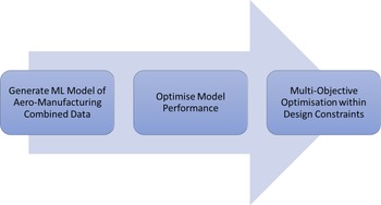
The main purpose of this study was to explore the impact of considering manufacturing characteristics in aircraft wing design through machine learning and optimisation-based methodology. The study was conducted in two main steps: first, carrying out ML modelling and MOO after including the manufacturing data in the aerodynamic performance dataset; and second, observing the changes in the optimal design conditions after including data concerning changes in the manufacturing conditions.
A diagram showing the approach taken for this study is shown below in Fig. 2.
Diagram showing study approach.

The same study approach was used twice for this study – once for optimisation without considering changes in rib design (i.e. without including spar positions as a variable) and once for optimisation with changes in design. This was because both study objectives had the same end goal of performing MOO to analyse the relationships between different involved variables, and the same process approach was required to meet that goal.
The main difference of the methodology of this study compared to other surrogate-based optimisation design methodologies was that the surrogate modelling process was conducted through non-parametric models as opposed to parametric models used in previous studies [Reference Martins, Li and Bouhlel23, Reference Shyy, Haftka, Mack and Goel24]. Even though the choice between parametric and non-parametric models cannot be determined a priori without testing, we chose XGboost as a non-parametric solution to include in our workflow. We based our choice on our experience, and also the versatility non-parametric models can have for any given dataset. A badly tuned parametric model can have a worse performance when compared to a non-parametric model. We also wanted to develop a generic methodology suitable for a range of different engineering design problems. Furthermore, we wouldn’t like to set an upper threshold to the number of variables contained within a dataset since some parametric models, such as Kriging, start to require a lot of effort to train and tune for multidimensional datasets, above 15 variables. It is the authors’ opinion that the proposed framework can satisfy many different design problems with no effort from the user to tune any models. This was especially necessary as the scope of this study was to include manufacturing and aerodynamic performance characteristics together, and including assumptions about the parametric relationships between manufacturing and aerodynamic performance characteristics may berisky.
The first step necessary to enable this approach was to generate an ML model of the combined aero-manufacturing dataset. This step needed to be completed first not only because it was related directly to one of the study objectives, but also because the successful prediction of targets within the given dataset was necessary to do MOO. MOO using the KanGAL software required the objective functions (the target variables) to be expressible in terms of the input variables, which needed to be achieved by building an ML model that predicted the output target based on the chosen input variables. Only once this was accomplished to a satisfactory degree could the optimisation process begin.
4.1 Generation of ML models
Before ML models could be generated, the provided data needed to be suitably filtered and processed. The data for modelling and optimisation without including spar positions was provided as a set of 3,060 points on simulated aerodynamic and manufacturing data for a single pair of spar positions (front spar position 12%, rear spar position 65%). The extra data for additional spar positions, however, was only available for simulated aerodynamic data. The bump amplitude values were the same for all of the simulations, and there were manufacturing data for each given bump amplitudes available from the previous data, so the same manufacturing data was used for different spar positions when including the spar positions as the variables. The total number of datapoints for combined spar positions was
 $3,060\times 9$
= 27,540 points.
In the initial data on aerodynamic performances and corresponding manufacturing characteristics, there were 21 different values and 2 loss functions. We decided that only several of the 21 values should be prioritised in the modelling process, as some of the values were dependent on other variables and time limitations on the study also needed to be considered. Thus, the data was filtered to include only the following variables:
-
• Alpha, meaning the angle-of-attack on the rib
-
• Mach number (Mach), representing the speed of airflow on the rib
-
• Drag Count, a measure for drag on the rib
-
• L/D, the ratio between lift generated by the rib and the drag it encounters
-
• Bump Amplitude (BumpAmp), a measure for the deviation in manufactured airfoil from nominal design
-
• Cpk, an index measuring the manufacturing capability
-
• Price of manufacturing a certain rib
-
• Manufacturing Process (MP) used (among three choices)
-
• Positions of front and rear spars (only for modelling and optimisation including spar positions)
-
• Mission performance = L/D + 1/DragCount as one target objective
-
• Manufacturability = 1,000/Price as the other target objective
It is important to note here that for the first study objective (modelling and optimisation without spar positions) the spar positions were fixed values (front spar position 12%, rear spar position 65%).”
This was because the dataset including spar positions were simulated for the same combination of aerodynamic input variables, creating extra data points for the same aerodynamic variable combinations whose differences from the original data could not be explained without including the changes in spar positions. This duplicity of data points for the same aerodynamic input combination resulted in errors during the training procedure for the first study. The combined dataset combinations with spar positions included was only used for the second study objective.
The next step was to select the combination of input and output variables for the modelling process. In an ideal situation with sufficient time and resources, the modelling could be done for all combinations of input and output variables, and the performances of all models could be analysed. In the scope of this study, however, Cpk and L/D were not considered as an input variable because they acted as constraints in the optimisation problem, and thus needed to be modelled by other inputs in order to be able to construct the optimisation problems correctly. Mission performance and manufacturability were the target objectives, and by the same logic, Drag Count (which was used to calculate Mission Performance) and Price (which was used to calculate Manufacturability) were excluded from being inputs as well. This left alpha, Mach, BumpAmp, MP, FS (front spar position) and RS (rear spar position), which were used as the input variables for modelling.
Then the ML models could be generated with the chosen set of input and output variables. To do this, the data needed to be parsed into a format used internally by XGBoost in order to be processed. For training and testing the model, the provided data was split randomly (the weight of the split being 7:3 with training being 7) into training and testing datasets before being used to train all models with different hyperparameter sets to compare their performances. The resulting models were saved, and the values of predictions and the corresponding labels (true values) were saved separately as well, which were used to calculate the modelling performance.
4.2 Optimisation of model performance – Hyperparameter tuning
The next step after modelling was to analyse the performance of the model and optimise the hyperparameter inputs for the modelling process. XGBoost offers various hyperparameters which influence the performances or even the type of model, to enable users to test a wider variety of conditions and tune the software for their specific purposes. For this study, there were four main hyperparameters that were altered and compared for their performance:
-
• Booster, which decides the what kind of modelling XGBoost will perform – the three choices were gbtree (regression tree), gblinear (generalised linear regression), and DART. For DART boosting, the hyperparameter drop_rate was set to 1, which makes it equivalent to random forests.
-
• Num_rounds, which decides how many boosting rounds to do – this hyperparameter was varied from 10 to 100 in spaces of 10.
-
• Eta, which is the weight of the sum of new features against the existing tree features – this hyperparameter was varied from 0.2 to 1 in spaces of 0.2.
-
• Max_depth, which is the maximum depth of each tree (i.e. number of splits) – this was varied from 2 to 4.
In order to evaluate the performance of these models, several methods and metrics were defined and used for evaluation of the models. The list of methods are shown as follows (the implementation of the evaluation metrics were imported from the sklearn.metrics library in Python):
-
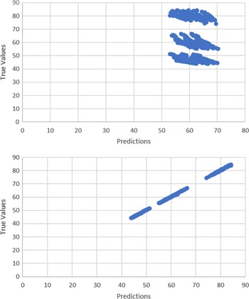
• Visual evaluation – creating the scatterplot of predicted vs real values of a modelling result to see if the scatterplot was linear (see Fig. 3 for more details)
-
• Mean Squared Error – calculating the mean squared error between prediction and real values to evaluate the absolute scale of error, is best when minimised
-
• % Accuracy – calculating the error between prediction and real values as a percentage of the corresponding real value, is best when minimised
-
• Adjusted R2 Score – calculating the adjusted r2 score for prediction vs real values to evaluate the degree of deviation between the two, is best when maximised (maximum is 1)
Comparison of bad scatterplot (above) and good scatterplot (below).

The three calculatable evaluation metrics were calculated for every modelling iteration, and the values of these metrics were recorded in a separate sheet for comparison. Based on the values of the scores, if they were good, the scatterplot of prediction against real values were evaluated to ensure that there were no wrong behaviours or unexpected errors that contributed to a good metric but bad model performance in real life.
It is worth noting that the goal of this hyperparameter tuning was to find a set of working hyperparameters that was able to model all necessary input and output variable combinations with high accuracy, not necessarily find the very best model performance for a single combination. This was due to the constraints on time and resources available for the study. An ideal set of hyperparameters would be able to model for all combinations of inputs and outputs perfectly, but in exploring the hyperparameters to find optimal values for the dataset itself, a set of model hyperparameters that could predict without compromising accuracy significantly for any of the combinations could be considered a good set of hyperparameters.
4.3 Multi-objective optimisation within design constraints
Once the model building process was complete, and the hyperparameters for accurately modelling all necessary input and output combinations were found, the last step of the whole study was to run the MOO and analyse the results.
The constraints and the list of variables and objectives needed to be clearly defined before the optimisation could be run. The main target objectives, as explained previously, were mission performance and manufacturability. The problem space also had two main constraints:
-
• Limits on value of Cpk due to manufacturing constraints: 1.33<Cpk<2
-
• Limits to not harm aerodynamic performance: L/D > 64.325
Verified ML models for targets and constraints were translated into a format that could be incorporated into the nsga-ii software. This process was necessary because the software for XGBoost was in python, while the KanGAL software for nsga-ii was coded in C. This was achieved through parsing of the dump files generated from the selected models, which contained all of the decision criteria and weights in each tree, using an open-source library called m2cgen. This parsing was tested to prove it produced the same results as loading the model before it was incorporated into nsga-ii.
After loading all the constraints and objectives into the nsga-ii software, the limits on variables themselves were defined according to the maximum and minimum values present within the given dataset:
-
• 2.1<alpha< 2.4
-
• 0.71<Mach<0.74
-
• 0.32<BumpAmp<2
-
• MP = 1,2,3
-
• 0.1<FS<0.14
-
• 0.63<RS<0.67 (FS and RS are in decimals as the values are position of spars along the rib in % of total length)
The MOO also required setting of other variables, such as population size and number of generations. The population size of the algorithm was set to 50 following the recommended population size of max {50,10n}, with n being the number of variables in the optimisation problem. The number of generations was set to 35 after conducting a first-round MOO, which showed from the optimisation history that the values of MOO converged at that point and showed no change afterwards. Effects of other indexes in the nsga-ii software were not explored due to time constraints, and their values were fixed. The list of indexes and their values are as follows:
-
• cross-over probability (0.5)
-
• mutation probability for real-coded vectors (0.1)
-
• distribution index for real-coded crossover (50)
-
• distribution index for real-coded mutation (250)
The limits on real-coded values were set to be rigid in the optimisation.
The MOO was conducted multiple rounds under same conditions to generate more population of results, and the results were compiled together to create the complete history and the pareto fronts of the optimisation. These pareto fronts were further analysed using Cambridge Advanced Modeller (CAM) software and was mainly used in this instance to generate the parallel coordinates plots of the pareto points.
5.0 Results and discussion
5.1 First study: Modelling and multi-objective optimisation without spar positions
5.1.1 ML modelling of objective variables
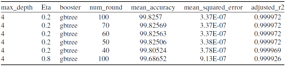
The first ML modelling was predicting the objective functions (mission performance and manufacturability) from the input variables alpha, Mach, BumpAmp and MP. The results of the modelling are shown in Table 1 and Fig. 4. The five models with best metrics are shown in Table 1.
Evaluation metrics for ML models of mission performance

Scatterplot of predictions against true values for mission performance without spar.

The best performing set of hyperparameters are shown to be max_depth = 4, eta = 0.8, booster = gbtree, num_round = 100, and the metric values are: mean_accuracy = 99.847%, mean_squared_error = 0.01987, and adjusted r2 score nearly 1. The resultant scatterplot of predictions against real values for this set of hyperparameters is shown in Fig. 4.
As it can be seen from the scatterplot, the prediction values match the true values very well. It can be said that this set of modelling hyperparameters performed very well in predicting the Mission Performance correctly.
Similar results are shown for predicting manufacturability with the given inputs.
In Table 2, the values evaluation metrics for the best performing conditions in mission performance was included to see the difference from the best results, and it can be seen that the performance of the model varies very little (approximately 0.15% in mean accuracy and almost no difference in adjusted r2 score). To verify whether manufacturability could also be predicted with the best performing conditions for mission performance (from this point onwards, these conditions will be referred to as the “base set of hyperparameters”), the scatterplot for manufacturability for the same modelling conditions is shown in Fig. 5.
Evaluation metrics for ML models of manufacturability

Scatterplot of predictions against true values for manufacturability without spar.

It can be seen that the base set of hyperparameters, which gave the best model performance for mission performance, also gave very good results for predicting manufacturability.
5.1.2 ML modelling of constraint variables
The next stage in ML modelling was modelling the constraints (Cpk and L/D) using the chosen inputs (alpha, Mach, BumpAmp and MP). The table of metrics for best-performing hyperparameters for predicting L/D is shown in Table 3.
Evaluation metrics for ML models of L/D

It can be seen that the base set of hyperparameters are present as well. Plotting the scatterplot of predictions against real values for L/D of the model generated with base set of hyperparameters is provided in Fig. 6.
Scatterplot of predictions against true values for L/D without spar.

It can be seen from the scatterplot that the base set of hyperparameters perform very well in predicting values of L/D as well.
Lastly, the table for models with top evaluation metric values for predicting Cpk is shown in Table 4.
Evaluation metrics for ML models of Cpk

Scatterplot of predictions against true values for Cpk without spar.

Complete history (above) and resulting pareto front(below) for MOO without spar positions.

The base set of hyperparameters can be seen here as well, which indicates that models using the base set of hyperparameters may be able to predict all of the constraints and objectives well. To test this, the scatterplot of predicted vs real values for models predicting Cpk using base set of hyperparameters is shown in Fig. 7.
It can be seen from the scatterplot that the model with base set of hyperparameters performed very well in predicting Cpk. This proved that the base set of hyperparameters may be used in modelling all of the constraints and objective functions when modelling without considering spar positions as an input variable.
5.1.3 Multi-objective optimisation results
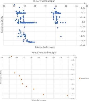
The next step was to run the multi-objective optimisation using the trained ML models to find the trade-off relationships. The MOO was conducted for 10 repetitive iterations under same optimisation conditions to collect more data points before the whole collected history was filtered to find the pareto front. The whole history and resulting pareto front of the MOO without spar positions is shown in Fig. 8.
The values of mission performance and manufacturability are shown as negative due to the nature of the optimisation algorithms, which requires all objective functions to be defined as minimisation problems. Thus, the ideal front of this graph is towards the bottom-left, where the absolute values of mission performance and manufacturability are at maximum.
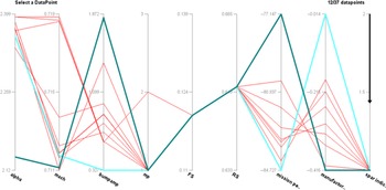
From the pareto front it can be seen that there is a clear trade-off relationship between the two objectives, which was something to be expected. It can also be seen that the intermediate values between the two extremes could give reasonably high values for both target objectives. To analyse the pareto front more effectively, the points on the pareto front were plotted on the parallel coordinates system (see Fig. 9).
Parallel coordinates plot of pareto front without spar.

In Fig. 9, the spar index is an arbitrary variable which indicates whether the values shown in the graph were optimised with spar positions or not. Also, the axes for the target objectives are negative – the higher the value of the two target objectives are, the lower on the graph they are located.
There were several things to note from this parallel coordinates plot. First, the trade-off between mission performance and manufacturability is visible on the plot as well, shown by the series of intersecting lines between the two axes, and it could be seen that there are choices which have reasonably good values for both target objectives. Also, the highest observed value of manufacturability in the pareto front was 0.416 (highlighted in dark green), which corresponded to a price of £2,404 per rib. The extreme values for each target objective are highlighted in dark green and sky blue, and it can be seen that the bump amplitudes for those values vary massively, which could be an explanation for the deviation as bump amplitude can be seen a measure of the manufacturing precision. It was also noticeable that almost all of the optimal operating conditions were focused on high values of alpha while operating conditions for Mach number were clustered around two values – 0.7187 and 0.7118.
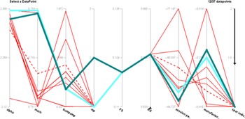
It can also be seen that almost all optimal manufacturing conditions indicated Manufacturing Process 1 – there were no points which considered manufacturing process 3 as a choice. Lastly, comparison of two points with the nearly the same bump amplitude but different manufacturing process showed that manufacturing process 2 had higher mission performance but lower manufacturability, and had a lower alpha as its operating condition, as shown in Fig. 10.
Comparison between two manufacturing processes for MOO without spar.

5.2 Second study: Modelling and multi-objective optimisation including spar positions
The ML modelling results of objectives and constraints with spar positions were analysed in the same way as the modelling without spar positions were.
5.2.1 ML modelling of objective variables
The table of evaluation metrics for modelling mission performance with the chosen inputs including spar positions are shown in Table 5.
Evaluation metrics for ML models of mission performance with spar

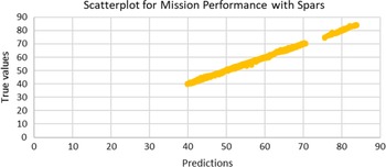
It is worth noting that the best performing hyperparameters for predicting mission performance with spars is the same as those for predicting without – namely, the base set. The scatterplot of prediction against real values for this base set model is shown in Fig. 11.
Scatterplot of predictions against true values for mission performance with spar.

It can be seen that the scatterplot also indicates a good performance of the model, and that this base set is an acceptable set of hyperparameters for predicting mission performance with spar positions as well.
Next wasmodelling manufacturability with spar positions. The evaluation metrics is shown inTable 6.
Evaluation metrics for ML models of manufacturability with spar

Scatterplot of predictions against true values for manufacturability with Spars.

The evaluation metrics for base set is shown here as well, and it can be seen that the difference in accuracy is even smaller than it was for the case of predicting manufacturability without spars using base set of hyperparameters. The scatterplot for this model is shown in Fig. 12.
It can be seen that the base set of hyperparameters also performed well in the predictions.
5.2.2 ML modelling of constraint variables
The evaluation metrics for modelling L/D with spars included in input variables are shown in Table 7.
Evaluation metrics for ML models of L/D with spar

Table 7 also shows the base set of hyperparameters as the best-performing of all tested combinations of model hyperparameters, with over 99.5% mean accuracy of prediction values. The corresponding scatterplot of the model is shown in Fig. 13.
Scatterplot of predictions against true values for L/D with spars.

The scatterplot also indicates a good performance of the model in predicting L/D with spar positions as inputs.
Finally, ML modelling was done for predicting Cpk from the given inputs including spar positions. The resulting evaluation metrics are shown in Table 8.
Evaluation metrics for ML models of Cpk with spar

It is necessary to mention that the adjusted r2 values in the table, shown as 1, is not actually 1.0 – rather, it is shown that way due to the number of significant digits. But the model with base hyperparameters still seems to perform very well according to the evaluation metrics.
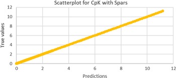
The scatterplot of the model with base hyperparameters is shown in Fig. 14.
Scatterplot of predictions against true values for Cpk with spars.

The scatterplot also indicates a good model performance using the base set of hyperparameters.
Based on the results of all of the ML model evaluations shown in Fig. 14, the base set of hyperparameters – max_depth = 4, eta = 0.8, num_rounds = 100, booster = gbtree – was set as the final modelling set of hyperparameters for all modelling processes to be used in the optimisation process.
Other noteworthy trends in the evaluation metrics observed during running different modelling scenarios included:
-
• out of the three boosting methods, gbtree performed the best
-
• increasing number of boosting rounds increased the accuracy of prediction, although it was seemingly more effective for increasing the accuracy in mission performance than manufacturability
-
• Increasing max depth improved the accuracy of the models
It may be noticeable that there are potential improvements in evaluation metrics from the base set of hyperparameters for the targets or constraints. However, the difference in performance varied very little, and as the goal of the hyperparameter tuning was to find a set of hyperparameters that could perform well in all combinations, the difference in performance was not analysed closely in this study.
It is worth mentioning again at this point that the full dataset was split randomly into training and testing dataset before each model was trained to prevent the potential problem of overfitting. The same training was also tested several times, and each time the models performed similarly well in predicting the data (with different randomised training datasets).
5.2.3 Multi-objective optimisation results
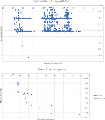
The same method of analysis was used for MOO with spar positions as well, and the two results were compared against each other to see the effects of including spar positions in the optimisation. As before, the ML models with base hyperparameters were selected as the objective and constraints for the MOO algorithm, and the MOO was re-iterated 10 times to collect more data points for the pareto front. The resulting complete history and pareto front are shown in Fig. 15.
The complete history (above) for MOO with spar positions and the pareto plot (below) for MOO with and without spar.

One thing to note in the complete history plot is the difference in scale of the axes – in the complete history without spar, the smallest values for mission performance started around 60, whereas for history with spar the starting values are lower, and goes down to nearly 50.
Looking at the pareto fronts plotted together, one thing is clearly visible: the pareto fronts are located at different positions. The pareto front for MOO with spar is located slightly more to the upper-right hand side. This change in the position of the pareto front is a positive outcome, as it indicates that including the spar positions as a variable created a difference in what kind of optimal trade-off relationships are available between the two target objectives.
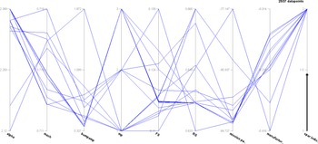
To analyse the pareto front generated by MOO with spar positions further, the pareto points were plotted on the parallel coordinates (see Fig. 16).
Parallel coordinates plot of MOO with spar.

One of the things immediately noticeable from the graph is that MOO with spar positions offers manufacturing process 3 as a viable choice. In the MOO without spar positions it was seen that manufacturing process 3 was not considered at all. This is another potential benefit of including spar positions as a variable, as it gives the rib design more flexibility in which manufacturing process to choose from.
The trade-off between mission performance and manufacturability is also observable here, but it is interesting to note that the values of mission performance and manufacturability seem to be more clustered around specific values than they were in the case of MOO without spars. There are a lot of values which have similar Mission Performances but varying Manufacturabilities, which was something that was not observed before in the MOO without spar, where the Mission Performance was more widely varied. This also may indicate a positive of including spar positions in MOO, as it seems to succeed in increasing the manufacturability for a same given value of mission performance through combination of other variables available, which was something that was not observed in MOO without spars.
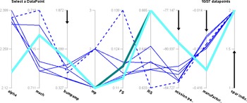
To compare both MOOs more equally, both parallel coordinates plots were filtered then plotted on the same graph. The filters applied were:
-
• limits on minimum mission performance at 80
-
• limits on minimum manufacturability at 0.17
-
• limits on maximum BumpAmplitude at 1.5
The resultant graph is shown in Fig. 17.
Comparison of MOO with and without spar positions.

The range of values for the operating conditions in within these limits are summarised in Table 9.
Comparison of ranges in operating conditions for pareto points

The comparison shows that MOO with spar position still offers more flexibility in manufacturing processes than MOO without spar position does. MOO with spars is more centred on a small range of bump amplitudes that are also lower than the values for MOO without spar positions, which could be interpreted as a positive result in terms of aerodynamic performance as it means the error between the nominal and manufactured aerofoil will be smaller and more controlled. The difference in manufacturability suggests that optimisation without spar positions yielded in more low-cost solutions.
It was alsoobserved, however, that small changes in just the spar positions affected the mission performance and manufacturability very little. Figure 18 highlights two different points with slightly different spar positions and nearly identical values for all other factors. This may potentially be due to the presence of less-dominating points in the pareto front with spar positions, or insufficient data points to analyse the relationship to a satisfactory level of confidence.
Two points (dark green and sky blue) with different front spar positions.

6.0 Conclusion and further considerations
6.1 Study conclusions
The main purpose of this study was to explore the impact of considering manufacturing characteristics in aircraft wing design through machine learning and optimisation-based methodology. The two specific objectives of the study were:
-
• Building a ML model that could predict aero-manufacturing combined data accurately
-
• Performing Multi-Objective Optimisation with and without the influence of spar positions to find the pareto fronts and analysing the effects of spar positions on the optimisation
The study wasa success in building a ML model for the combined aero-manufacturing data utilising XGBoost. The obtained model could predict the combined aero-manufacturing data with high accuracy and reliability, and verified the potential of combining the distant areas of mission performance and manufacturability to consider both factors at the same time. The MOO without spar positions as a variable found a visible trade-off region between high manufacturability and high mission performance, and offered choices of different combinations of manufacturability and mission performance, which can be adjusted according to different needs.
Comparison of MOO with and without spar positions resulted in a trade-off relationship between mission performance and manufacturability, which was different from the trade-off relationship found in MOO without spar positions. The difference in trade-off relationships showed that the inclusion of different variables in the modelling had the potential to find relationships that reflected the real world more accurately. It was also worth noting that the MOO with spar positions offered more flexibility in the choice of manufacturing processes available for a given design.
There was no clearly identified correlation between a small change in spar position and the optimal values for the target objectives; however, the range of bump amplitudes for solutions found by MOO with spar positions was lower and more focused than those found by MOO without spar positions.
6.2 Further considerations
There are also a number of things to be noted as potential future directions of this study.
First, while the study results suggested a meaningful results in modelling of the combined data, a further study on the optimisation with more repetitions and sufficient data could help add confidence to the findings of this study.
Also, there is the inherent uncertainty in the true “continuity” of variables analysed in this study to consider. For example, the locations of spar positions, considered to be truly continuous for this study context, can be subject to physical limitations in manufacturing or assembly. Exploration of this uncertainty can help the results of the study reflect the real world conditions better.
Another point for potential improvement of the current study is the fact that the structural stiffness of the discovered pareto fronts have not been simulated to verify that the corresponding points actually yield a viable wing structure. While a significant problem in the structural stiffness of the part is not expected as the ranges of variability in front and rear spar did not change the structural stiffness of the wing box since the aerodynamic loads do not change, it is definitely worth simulating the actual conditions to further validate the results of the study.
Last but not least, there are numerous other variables not considered in this study that could help build a more accurate model. For example, the necessary shape of the rib and its aerodynamic performance changes according to the position of a rib down the length wing – considering the changes in rib shape and performance according to its position along the wing as additional variables may provide richer interpretation of the design space and new opportunities for improvement.
Acknowledgements
The research leading to these results has received support by members of the consortium of the Advanced Product Concept Analysis Environment (APROCONE) project (Ref no. 113092), which was funded by the Aerospace Technology Institute (ATI) in the UK.