





1. Introduction
Rayleigh–Bénard convection has attracted considerable attention due to its ubiquity in nature and industry. It has been extensively investigated (Manneville Reference Manneville2006), from laminar cells to turbulence (Goluskin Reference Goluskin2016) and from water tanks to stars (Le Bars et al. Reference Le Bars, Lecoanet, Perrard, Ribeiro, Rodet, Aurnou and Le Gal2015). Many works on the convection of weakly compressible fluids apply the Boussinesq approximation (Bodenschatz et al. Reference Bodenschatz, Pesch and Ahlers2000). The equation of state (EOS) of the fluid is often assumed to be linear, leading to the simplest mathematical model of convection. However, nonlinearity of the EOS can be important in certain scenarios (Olsthoorn et al. Reference Olsthoorn, Tedford and Lawrence2021; Wang et al. Reference Wang, Calzavarini, Sun and Toschi2021).
For compressible convection models where the sound speed is required to be resolved, the complete nonlinear form of the EOS is usually applied in a wide range of industrial problems related to gases (Mayeli & Sheard Reference Mayeli and Sheard2021). Nevertheless, the class of fluids exhibiting a nonlinear EOS extends well beyond gaseous media. For weakly compressible fluids, a representative example is pure water at a temperature close to its maximum density point (with temperature
 $ \approx 277\,\mathrm{K}$
). The nonlinear part of the EOS plays a critical role in determining the temperature stratification of freshwater lakes during winter (Boehrer & Schultze Reference Boehrer and Schultze2008; Jansen et al. Reference Jansen2021), thus drawing interest in a quadratic EOS. Veronis (Reference Veronis1963) first conducted a linear stability analysis of a fluid layer with the EOS
 \begin{align} \rho =\rho _0\big [1-\beta (T-T_0)^2\big ] \end{align}
and Dirichlet boundary conditions for the top and bottom boundary temperatures. Here the density is
 $\rho$
and
 $T$
is the temperature, with
 $\rho _0$
and
 $T_0$
representing their respective reference values. The thermal expansion rate is denoted as
 $\beta$
. Two- and three-dimensional numerical simulations have been performed based on an EOS of this form, as reviewed by Wang et al. (Reference Wang, Zhou, Wan and Sun2019) and Olsthoorn et al. (Reference Olsthoorn, Tedford and Lawrence2021). These simulations typically show development of separate stably stratified and convective regions, closely resembling the division between radiative and convective zones in stars and thus lending astrophysical relevance (Le Bars et al. Reference Le Bars, Lecoanet, Perrard, Ribeiro, Rodet, Aurnou and Le Gal2015).
Salt solutions such as seawater also have a nonlinear EOS (Sharqawy et al. Reference Sharqawy, Lienhard and Zubair2010; Nayar et al. Reference Nayar, Sharqawy, Banchik and Lienhard2016). McDougall (Reference McDougall1981) considered double-diffusive convection with a nonlinear EOS, noting that different convection activities can occur in two well-mixed layers because a given heat flux across the sharp interfaces causes different buoyancy fluxes, which can lead to entrainment in one direction. Kim et al. (Reference Kim, Moon, Wells, Wilkinson, Langton, Hwang, Granskog and Rees Jones2018) applied a nonlinear EOS to model saline melt ponds in the Arctic that are heated by radiative absorption. Their simulations show that convection in saline ponds is significantly different from that in freshwater ponds with the same internal heating. They applied a different quadratic approximation of the EOS motivated by practical temperature and salinity ranges observed in melt ponds:
 \begin{align} {\rho }={\rho _0}\big [1+{\alpha }(T-T_0)+{\beta }(T-T_0)^2\big ]. \end{align}
Here
 $\alpha$
and
 $\beta$
depend on the salinity, which is assumed to be uniform. Equation (1.2) is selected as the EOS in this paper because of the motivation for geophysical applications to melt ponds on Arctic sea ice. Furthermore, it provides a method to explore the transition for increasing nonlinearity between the linear EOS and (1.1) by varying
 $\alpha$
and
 $\beta$
. We demonstrate that the phase diagram of the convective instability can exhibit a discontinuous transition as the EOS varies. As the nonlinearity strengthens, the number of unstable regions first transitions from one to two, before reverting to one unstable region for large nonlinearity.
Many geophysical convective systems are driven by solar radiation (e.g. Farmer Reference Farmer1975; Toppaladoddi & Wettlaufer Reference Toppaladoddi and Wettlaufer2018; Yang et al. Reference Yang, Howland, Liu, Verzicco and Lohse2023; Huang et al. Reference Huang, Ouyang and Ding2025). The interaction between radiation and fluid dynamics in the environment occurs through two distinct mechanisms: thermal forcing as an internal energy source and forcing at the phase interface. For the former type, shortwave absorption dominates. A common treatment yields exponential decay of the heating source according to the Beer–Lambert law (Farmer Reference Farmer1975; Grace et al. Reference Grace, Stastna, Lamb and Scott2022), but the heating can exhibit distinct behaviours due to different media and basal properties. For substrates with significant reflectivity like ice, the absorption behaviour is modified by the upward reflected radiation flux (Taylor & Feltham Reference Taylor and Feltham2004). Here we use a two-stream absorption model proposed by Skyllingstad & Paulson (Reference Skyllingstad and Paulson2007) for melt ponds whose substrate is sea ice. Despite the adoption of a specific absorption model as the heat source, our results are expected to be qualitatively consistent with those obtained with other models with similar monotonicity of the heating profile.
The thermal boundary conditions also impact convection dynamics in geophysical settings. At radiatively forced gas–liquid interfaces such as atmosphere–lake or atmosphere–pond interfaces, the heat transfer depends on the net sum of various components, including incoming longwave and shortwave radiation, reflected fluxes, longwave radiative cooling, sensible and latent heat fluxes, as well as conductive fluxes (Maykut & Untersteiner Reference Maykut and Untersteiner1971; Taylor & Feltham Reference Taylor and Feltham2004). In many settings the general thermal boundary condition can be approximated by linearised Robin conditions when the temperature variation is small compared with a reference value (see, e.g. Hitchen & Wells Reference Hitchen and Wells2016). A dimensionless Biot number
 $Bi$
can be used to measure the effective thermal exchange with the gas relative to the conductive flux in the liquid. Formally resembling the Newtonian cooling condition, the Robin condition describes a regime that transitions between the adiabatic and perfectly conducting extremes as
 $Bi$
varies from
 $Bi\rightarrow 0$
to
 $Bi \rightarrow \infty$
. Hurle et al. (Reference Hurle, Jakeman and Pike1967) considered Rayleigh–Bénard convection in a pure liquid with a Robin condition for temperature at the upper boundary. Clarté et al. (Reference Clarté, Schaeffer, Labrosse and Vidal2021) explored the effects of a Robin condition on thermal convection in a rotating spherical shell. Their results show that a Dirichlet or Neumann condition can be applied to replace the Robin condition only when
 $Bi$
lies in an appropriate limit. The Robin condition has also been applied at the solid–fluid interface in engineering problems to simulate more realistic heat transfer (e.g. Errera & Duchaine Reference Errera and Duchaine2016). Besides pure fluids, Hitchen & Wells (Reference Hitchen and Wells2016) showed that
 $Bi$
can significantly influence the critical wavelength and depth of convection for a deep porous medium. Therefore, setting an appropriate condition is important for understanding realistic convective instability. Here we employ a Robin condition on the temperature at the upper boundary. This enables our work to provide insights for a broader range of environmental and engineering problems including both natural and forced cooling (Beckermann et al. Reference Beckermann, Gu and Boettinger2000).
Here we consider the impact of the quadratic EOS (1.2) on convective instability in a fluid layer internally heated by radiative absorption with a Robin condition for temperature at the top and a Dirichlet condition at the bottom. Although this type of system has been simulated for selected parameter sets (Kim et al. Reference Kim, Moon, Wells, Wilkinson, Langton, Hwang, Granskog and Rees Jones2018), its linear and weakly nonlinear behaviour, along with broader parameter regimes, remain unexplored. A dimensionless parameter
 $\kappa _n$
is defined to quantify the relative importance of terms involving
 $\beta$
and
 $\alpha$
in the EOS (1.2). This work assumes that
 $\alpha \gt 0$
and
 $\beta \lt 0$
, so that the model directly represents saline melt ponds on Arctic sea ice (Kim et al. Reference Kim, Moon, Wells, Wilkinson, Langton, Hwang, Granskog and Rees Jones2018). We conduct most of the analysis and simulations in this paper with parameter choices motivated by this specific scenario, but expect the conceptual conclusions to apply more generally to a wider range of convective systems. The system exhibits different flow patterns with different
 $\kappa _n$
, giving rise to variation of the vertical heat transport. Both linear stability analysis and direct numerical simulations (DNS) show that two convective modes are possible within a certain window of
 $\kappa _n$
with different patterns of the dominant energy input. The transition region between them is stable. One of the modes for smaller
 $|\kappa _n|$
consists of strong ascending plumes from the lower boundary, and the other mode for larger
 $|\kappa _n|$
is dominated by weak subsiding plumes from the upper boundary. Both modes are possible for intermediate
 $\kappa _n$
. We also use weakly nonlinear analysis to understand the properties of the possible bifurcations.
The description of the idealised model is detailed in § 2. The methodology is discussed in § 3 with the base-state solution in § 3.1, and the linear stability analysis technique in § 3.2. We introduce the weakly nonlinear analysis method in § 3.3 and the DNS method in § 3.4. The stability results are demonstrated in § 4, including the linear stability and its validation in § 4.1, and weakly nonlinear results in § 4.2. Section 5 outlines the results from DNS for strongly nonlinear convection, consisting of two-dimensional cases in § 5.1 and three-dimensional simulations for representative parameter sets in § 5.2. Section 6 illustrates the main geophysical application of this model to melt ponds on Arctic sea ice. We conclude with a summary of the work in § 7.
2. Model
We consider a horizontally periodic fluid layer, which has a quadratic EOS and is internally heated by radiation absorption, as illustrated in figure 1. The fluid can be understood as an aqueous saline solution of uniform salinity at a temperature within a few degrees of the freezing temperature, with the complete EOS truncated to the lowest order of nonlinearity as given by (1.2), and reference temperature
 $T_0$
set to the temperature of the bottom boundary. For melt ponds,
 $T_0$
is the melting point, maintained by phase equilibrium. For other systems, it should be interpreted as the temperature of a basal thermal reservoir. Note that the coefficients of thermal expansion
 $\alpha \gt 0$
and
 $\beta \lt 0$
, meaning that the volume can either decrease or increase with temperature here due to the density anomaly. For a saline solution, the specific values of
 $\alpha$
and
 $\beta$
depend on the salinity.
With the Boussinesq approximation, the continuity equation, heat transport equation and momentum equation are written as
 \begin{align} {\boldsymbol{\nabla }}\boldsymbol{\cdot }{\boldsymbol{u}^*}=0, \\[-28pt] \nonumber \end{align}
 \begin{align} {\rho _0}c_p\left (\frac {\partial T}{\partial t^*}+{\boldsymbol{u}^*}\boldsymbol{\cdot }{\boldsymbol{\nabla }T}\right )=K{{\nabla} }^2T+R(z^*), \\[-28pt] \nonumber \end{align}
 \begin{align} {\rho _0}\left (\frac {\partial \boldsymbol{u}^*}{\partial t^*}+{\boldsymbol{u}^*}\boldsymbol{\cdot }{\boldsymbol{\nabla }\boldsymbol{u}^*}\right )=-{\boldsymbol{\nabla }}p^*+{\mu }{{\nabla} }^2\boldsymbol{u}^*-({\rho }-{\rho _0})g\boldsymbol{e_z}, \\[0pt] \nonumber \end{align}
where the
 $z^*$
direction is positive upward with
 $\boldsymbol{e_z}$
as the unit vector, and
 $R(z^*)$
represents the internal heat source from shortwave radiation absorption. The pressure is
 $p$
,
 $\mu$
denotes the dynamic viscosity,
 $c_p$
the specific heat at constant pressure,
 $K$
the thermal conductivity,
 $\boldsymbol{u}^*=u^*\boldsymbol{e_x}+v^*\boldsymbol{e_y}+w^*\boldsymbol{e_z}$
the velocity with horizontal unit vectors
 $\boldsymbol{e_x}$
and
 $\boldsymbol{e_y}$
, and
 $g$
the gravitational acceleration. The time is
 $t^*$
.
Diagram illustrating the model setting. Red curves show the monotonicity of the internal heat source
 $R(z^{*})$
and the background temperature profile
 $T(z^{*})$
. The dimensional boundary conditions are also shown.

For the heat source term, we adopt the two-stream radiation absorption model suggested for melt ponds by Skyllingstad & Paulson (Reference Skyllingstad and Paulson2007):
 \begin{align} R(z^*)=F_{SW}\sum _{m=1}^4P_mK_m\left [\textit{e}^{-K_m\left (H-z^*\right )}+a_b\textit{e}^{-K_m\left (H+z^*\right )}\right ]. \end{align}
Incoming solar radiation is spectrally partitioned into four wavelength bands, each characterised by a fractional energy content
 $P_m=\{0.481, 0.194,0.123,0.202\}$
and an absorption coefficient
 $K_m=\{0.18,3.25,27.5,300\}\,\mathrm{m}^{-1}$
for
 $m=1,2,3,4$
, which governs the exponential attenuation of radiation with depth. In addition to the downward flux, the model also accounts for upward reflection from the pond–ice boundary, parameterised by an albedo coefficient
 $a_b=0.7$
.
Within the characteristic convective time scale of interest, phase changes and the resulting boundary movement are assumed to be negligible for both the bottom and top boundaries. The bottom boundary is assumed to be a no-slip wall with a constant temperature, so
 \begin{align} T=T_0,\enspace \boldsymbol{u}^*=\boldsymbol{0},\quad \mbox{at } z^*=0. \end{align}
For a melt pond, this represents a solid–liquid phase boundary at the melting temperature. The top boundary is treated as a free-slip wall, neglecting external stress. We thus focus on natural convection rather than forced convection. The general heat exchange condition at the top of a melt pond is influenced by a combination of shortwave radiation, longwave radiation, sensible heat flux and latent heat flux, while a longwave cooling term from the Stefan–Boltzman law introduces nonlinearity. For simplicity, this work instead assumes that the deviation of the boundary temperature from the reference value remains small, and we employ a linearised heat transfer condition at the top yielding a Robin condition (c.f. Hitchen & Wells Reference Hitchen and Wells2016). In summary,
 \begin{align} w^*=0,\qquad \frac {\partial u^*}{\partial z^*}=\frac {\partial v^*}{\partial z^*}=0,\qquad K\frac {\partial T}{\partial z^*}=-F_0 -\gamma (T-T_0),\quad \mbox{at } z^*=H, \end{align}
where the fluid layer has depth
 $H$
. Here,
 $F_0$
is the reference flux and
 $\gamma$
is the coefficient of the linear term obtained from a Taylor expansion of the full energy flux balance. We have neglected the vertical surface motion caused by a phase change such as evaporation, along with any possible deformation of the upper surface. To measure the strength of the internal radiation forcing, we define the average absorption as
 \begin{align} Q_0=\frac {1}{H}\int _0^H R(z^*)\textit{d}z^*. \end{align}
The lateral boundaries are assumed to be periodic to facilitate theoretical analysis, because the horizontal scale of many radiatively driven convective systems is much larger than their depth. For example, Arctic melt ponds have typical widths of
 $O(10\,\mathrm{m})$
versus a depth of
 $O(0.1\,\mathrm{m})$
(Kim et al. Reference Kim, Moon, Wells, Wilkinson, Langton, Hwang, Granskog and Rees Jones2018).
Convection with the nonlinear EOS (1.2) adds an extra dimension to the usual parameter space for internally heated convection. As usual, the relative significance of viscous versus thermal diffusion is characterised by the Prandtl number
 $ \textit{Pr}=\nu /\kappa _T$
, where
 $\kappa _T={K}/{\rho _0c_p}$
and
 $\nu =\mu /\rho _0$
. We here consider
 $ \textit{Pr}$
values of order
 $10$
, relevant to cold water. It is customary to quantify the strength of buoyancy effects versus viscous and thermal dissipation using a Rayleigh number
 $\Delta \rho g H^3/\rho _0 \kappa _T \nu$
, where
 $\Delta \rho$
is the characteristic density difference controlling the buoyancy force. Here
 $\Delta \rho$
can have contributions from the linear and nonlinear variations of density with temperature in the EOS (1.2). The linear contribution naturally yields
 $\Delta \rho =\rho _0 \alpha \Delta T$
for a temperature scale
 $\Delta T=Q_0 H^2/K$
controlled by the balance of internal heating and conduction, resulting in the linear Rayleigh number
 \begin{align} Ra=\frac {\alpha Q_0H^5g}{K\kappa _T\nu }. \end{align}
The nonlinear contribution has
 $\Delta \rho =\rho _0 \beta \Delta T^2$
. Here we choose to express the relevant Rayleigh number for nonlinear density change as
 \begin{align} \frac {\Delta \rho \,gH^3}{\rho _0 \kappa _T \nu } = \frac {\beta Q_0^2gH^7}{K^2 \kappa _T \nu }=\kappa _n\,\textit{Pr}\,\textit{Ra}^2, \end{align}
in terms of
 $ \textit{Pr}$
,
 $ \textit{Ra}$
and a newly introduced parameter
 \begin{align} \kappa _n=\frac {\beta \kappa _T^2}{\alpha ^2gH^3}, \end{align}
which is a measure of the nonlinearity of the non-dimensional EOS. Note that
 $\kappa _n$
has been defined here to be independent of the nominal heating rate
 $Q_0$
, and only depends on material properties and geometry. The relevant dependence of
 $\Delta \rho$
on
 $\Delta T$
and, hence,
 $Q_0$
is carried via the
 $ \textit{Ra}^2$
term in (2.9). Hence, the significance of nonlinearity will also increase with
 $ \textit{Ra}$
(for example, due to increased internal heating). For simplicity, here we consider cases with
 $ \textit{Ra} \gt 0$
and
 $\kappa _n\lt 0$
. Where specific dimensional parameters are used in the following, we set the constant values
 $\kappa _T=1.5\times 10^{-7} \,\mathrm{m^2\,s^{-1}}$
,
 $g=9.81\,\mathrm{m\,s^{-2}}$
and
 $H=0.1\,\mathrm{m}$
. The values of
 $\alpha$
and
 $\beta$
depend on the specific material considered. For melt ponds on sea ice, we consider a saline solution where
 $\alpha$
and
 $\beta$
are evaluated at a reference temperature of the melting point. Hence,
 $\kappa _n$
will vary with the absolute salinity
 $ \textit{SA}$
of the pond water, which impacts
 $\alpha$
and
 $\beta$
. There is significant monotonic variation with
 $4.9\times 10^{-9}\lt -\kappa _n \lt 2.6 \times 10^{-3}$
as the salinity varies between
 $1\,\mathrm{g\,kg}^{-1} \lt SA \lt 23.9\,\mathrm{g\,kg}^{-1}$
, using data from McDougall & Barker (Reference McDougall and Barker2011).
When non-dimensionalising, Kim et al. (Reference Kim, Moon, Wells, Wilkinson, Langton, Hwang, Granskog and Rees Jones2018) found that the diffusion scale yields poorly conditioned and inefficient numerical simulations of this model when there is vigorous convection. Therefore, to maintain consistency between the scaling in the theoretical calculations and the numerical simulations, we introduce scales depending on a dimensionless parameter
 $\tau = (Ra\,Pr )^{1/3}$
following their work. We see below in (2.12) and (2.13) that
 $\tau$
plays the role of a dimensionless Péclet number, controlling the significance of advection versus thermal diffusion. Using
 $\tau$
we non-dimensionalise using a characteristic length scale
 $H$
, characteristic time scale
 $ H^2/\kappa _T\tau$
, velocity scale
 $\kappa _T\tau /H$
, temperature scale
 $T-T_0\sim Q_0H^2/K\tau$
, density difference scale
 $ \rho _0 \alpha Q_0H^2/K\tau$
and pressure difference scale
 $\rho _0 \kappa _T^2\tau ^2/H^2$
. The resulting dimensionless system is
 \begin{align} \boldsymbol{\nabla }\boldsymbol{\cdot }\boldsymbol{u}=0, \\[-28pt] \nonumber \end{align}
 \begin{align} \frac {\partial \theta }{\partial t}+\boldsymbol{u}\boldsymbol{\cdot }\boldsymbol{\nabla }\theta = \frac {1}{\tau } {\nabla} ^2\theta +r(z), \\[-28pt] \nonumber \end{align}
 \begin{align} \frac {\partial \boldsymbol{u}}{\partial t}+{\boldsymbol{u}}\boldsymbol{\cdot }{\boldsymbol{\nabla }\boldsymbol{u}}= \frac {\textit{Pr}}{\tau }{\nabla} ^2\boldsymbol{u}-\boldsymbol{\nabla }p-\big (\theta +\kappa _n\tau ^2\theta ^2\big )\boldsymbol{e_z}, \\[-28pt] \nonumber \end{align}
 \begin{align} \boldsymbol{u}=0,\qquad \theta =0, \quad \mbox{at} \ z=0, \\[-28pt] \nonumber \end{align}
 \begin{align} w=0,\qquad \frac {\partial {u}}{\partial {z}}= \frac {\partial {v}}{\partial {z}}=0, \quad \mbox{at} \ z=1, \\[-28pt] \nonumber \end{align}
 \begin{align} \frac {\partial \theta }{\partial z}=-f\tau -\textit{Bi}\,\theta \quad \mbox{at} \ z=1, \\[0pt] \nonumber \end{align}
where
 $\boldsymbol{u}$
,
 $\boldsymbol{x}$
and
 $t$
correspond to the dimensionless values,
 $\theta = (T-T_0 )K\tau /Q_0H^2$
,
 $r=R/Q_0$
, and
 $\tau /Pr$
plays a similar role to the Reynolds number in (2.13). Two other dimensionless parameters,
 \begin{align} f=\frac {F_0}{Q_0H}, \qquad Bi=\frac {\gamma H}{K}, \end{align}
naturally emerge during the non-dimensionalisation of the Robin boundary condition. With this particular non-dimensionalisation, the nonlinearity of the EOS plays a role in the buoyancy term depending on
 $\kappa _n \tau ^2$
, where
 $\tau =(\textit{Pr}\,\textit{Ra})^{1/3}$
. Note that although the parameter space of the model is complex, the discussion in the main text is primarily restricted to the influence of
 $\kappa _n$
,
 $ \textit{Ra}$
and
 $ \textit{Pr}$
, which in turn directly impact
 $\tau =(\textit{Pr}\,\textit{Ra})^{1/3}$
. Some sensitivity tests on
 $f$
and
 $Bi$
are presented in Appendix C. In summary, the model becomes a Rayleigh–Bénard convection problem adjusted with one Robin condition, internal radiative heating and a nonlinear buoyancy force. Numerous studies on Rayleigh–Bénard convection (Goluskin Reference Goluskin2016) have shown that stability analysis can provide useful information.
3. Analysis and simulation methods
This section discusses the methods used: namely linear stability analysis, weakly nonlinear analysis and DNS. We add a perturbation to a steady and conductive state. We should acknowledge that, for many radiatively heated geophysical objects (such as lakes, ponds, oceans, etc.), a strictly stationary background state does not exist because of the diurnal and seasonal fluctuations of solar radiation. This work assumes that the time scale of thermal convection (if it can happen) is much smaller than the time scale
 $t_d$
of diurnal evolution. The specific form of the stability theory may depend crucially on the choice of the background state. For simplicity, we consider a system with a static base state.
3.1. Base-state solution
For a steady heat source, a static background temperature profile is obtained by solving the heat conduction equation without time derivatives. The dimensionless heat source is
 \begin{align} r(z)=\sum _{m=1}^4\frac {P_m k_m}{\zeta _b}\big [\textit{e}^{-k_m(1-z)}+a_b\textit{e}^{-k_m(1+z)}\big ], \end{align}
where
 $k_m=K_mH$
and
 $\zeta _b$
is a normalisation constant satisfying
 \begin{align} \zeta _b=\sum _{m=1}^4 P_m \big (1+a_b \textit{e}^{-k_m}\big )\big (1-\textit{e}^{-k_m}\big ). \end{align}
Then the steady solution of (2.12) with the source term (3.1) and boundary conditions (2.14) and (2.16) is
 \begin{align} \frac {\theta }{\tau }\equiv \frac {\theta _0}{\tau }=c_1z+\sum _{m=1}^4\frac {P_m}{\zeta _b k_m}\big [\left (1+a_b\right )\textit{e}^{-k_m} -\textit{e}^{-k_m(1-z)}-a_b\textit{e}^{-k_m(1+z)}\big ], \end{align}
where
 \begin{align} c_1=\frac {-f+\sum _{m=1}^4 ({P_m}/{\zeta _b})\left (1-a_b \textit{e}^{-2k_m}\right )-Bi\sum _{m=1}^4 ({P_m}/{\zeta k_m})\left [\left (1+a_b\right )\textit{e}^{-k_m}-1-a_b\textit{e}^{-2k_m}\right ]}{1+Bi}. \end{align}
The dimensionless background temperature profiles
 $\theta$
scaled with
 $ \textit{Ra}$
and
 $ \textit{Pr}$
, and the corresponding internal heat source
 $r$
, when
 $Bi=1.4$
,
 $f=0.5$
,
 $k_m= [0.018,0.325,2.75,30]$
,
 $\zeta _b\approx 0.4178$
and
 ${P_m}/{\zeta _b k_m}=[63.9594,1.4287,0.1071,0.0161]$
.

Base-state temperature profiles are presented in figure 2 for selected parameters. Most of the heating power is concentrated close to the top boundary, which is a typical characteristic of solar radiation forcing in water. The temperature profile is non-monotonic, due to the internal heating and heat losses from the upper surface and cold isothermal lower boundary.
3.2. Linear perturbations
After perturbation (
 $\theta \rightarrow \theta _0+\theta _1$
,
 $p\rightarrow p_0+p_1$
), we omit the subscript
 $1$
on the perturbation for brevity. The governing equations and boundary conditions are
 \begin{align} \boldsymbol{\nabla }\boldsymbol{\cdot }\boldsymbol{u}=0, \enspace \frac {\partial \theta }{\partial t}+ w\frac {\partial \theta _0}{\partial z}+\boldsymbol{u}\boldsymbol{\cdot }\boldsymbol{\nabla }\theta = \frac {1}{\tau } {\nabla} ^2\theta , \\[-28pt] \nonumber \end{align}
 \begin{align} \frac {\partial \boldsymbol{u}}{\partial t}+{\boldsymbol{u}}\boldsymbol{\cdot }{\boldsymbol{\nabla }\boldsymbol{u}}= \frac {\textit{Pr}}{\tau }{\nabla} ^2\boldsymbol{u}-\boldsymbol{\nabla }p-(1+2\kappa _n\tau ^2\theta _0)\theta \boldsymbol{e_z}-\kappa _n\tau ^2\theta ^2\boldsymbol{e_z}. \\[-28pt] \nonumber \end{align}
 \begin{align} \boldsymbol{u}=0,\qquad \theta =0, \quad \mbox{at} \ z=0, \\[-28pt] \nonumber \end{align}
 \begin{align} w=0,\qquad \frac {\partial {u}}{\partial {z}}= \frac {\partial {v}}{\partial {z}}=0, \qquad \frac {\partial \theta }{\partial z}=-\textit{Bi}\,\theta ,\quad \mbox{at} \ z=1, \\[0pt] \nonumber \end{align}
where
 $\tau =(\textit{Ra}\textit{Pr})^{{1}/{3}}$
. As with three-dimensional classical Rayleigh–Bénard convection, an efficient method for computation of the critical Rayleigh number is to take the double curl of the momentum equation and reformulate as an eigenvalue problem with the Rayleigh number as the eigenvalue (by letting the time derivative be zero). This assumes that the growth rate of the critical state in the linearised system is zero, thereby excluding any oscillatory behaviour represented by a purely imaginary growth rate. Fortunately, our problem satisfies this assumption, which is validated by numerical simulations shown later.
The lateral boundary conditions in the
 $x$
and
 $y$
directions are periodic, so we set
 \begin{align} w=W(t,z)\textit{e}^{ik_1 x+ik_2 y},\qquad \theta = \varTheta (t,z)\textit{e}^{ik_1 x+ik_2 y}. \end{align}
Linearising (3.5) and (3.6), and using
 $\boldsymbol{\nabla }\times (\boldsymbol{\nabla }\times \boldsymbol{u} )$
, we obtain a system for
 $w$
and
 $\theta$
:
 \begin{align} \frac {\partial }{\partial t}{\nabla} ^2 w=\frac {\textit{Pr}}{\tau }{\nabla} ^2{\nabla} ^2 w + k^2\theta \big(1+2\kappa _n\tau ^2\theta _0 \big), \\[-28pt] \nonumber \end{align}
 \begin{align} \frac {\partial \theta }{\partial t}+ w\frac {\partial \theta _0}{\partial z} = \frac {1}{\tau }{\nabla} ^2\theta . \\[0pt] \nonumber \end{align}
Here
 $k^2=k_1^2+k_2^2$
. The boundary conditions are
 \begin{align} w=\frac {\partial w}{\partial z}=0\quad \mbox{at}\ z=0;\qquad w=\frac {\partial ^2 w}{\partial z^2}=0\quad \mbox{at} \ z=1, \\[-28pt] \nonumber \end{align}
 \begin{align} \theta =0\quad \mbox{at}\ z=0;\qquad \frac {\partial \theta }{\partial z}=-Bi\,\theta \quad \mbox{at}\ z=1. \\[0pt] \nonumber \end{align}
The two additional boundary conditions involving derivatives of
 $w$
arise from the boundary conditions on
 $u$
,
 $v$
and the incompressibility condition. Under the combined influence of the Robin boundary condition for temperature at the upper boundary, the fourth-order derivative of the velocity in the governing equation, and the more complex buoyancy term in the current system compared with classical problems, the usual Chebyshev spectral method is not the optimal numerical approach for this problem. Using too few modes results in significant numerical error, while increasing the number of modes leads to a substantial increase in the condition number of the coefficient matrix in the eigenvalue problem. Therefore, the basis functions for expanding
 $W$
and
 $\varTheta$
are here specially chosen, making a trade-off between orthogonality and numerical stability. The method demonstrates good performance in terms of convergence and numerical stability, and its prediction aligns well with the DNS results.
To maintain a coherent flow of presentation, we provide here a brief overview of the modified spectral method, while full details are given in Appendix A. We set
 \begin{align} W=\sum _{n=1}^N \textit{FM}_n\text{sin}(n\pi z), \qquad F(z)=2z-z^2, \end{align}
and
 \begin{align} \varTheta =\sum _{n=1}^N \varTheta _n\theta _n(z), \end{align}
where
 \begin{align} \theta _n = \sin {\lambda _n z},\qquad \lambda _n + \textit{Bi}\,\tan {\lambda _n}=0 \end{align}
are from a Sturm–Liouville problem.
Finally, we obtain an eigenvalue problem that can be formally written in an intuitive way:
 \begin{align} {\nabla} ^2{\nabla} ^2w=-k^2 \textit{Ra}\big \{1+2\kappa _n \textit{Pr} \textit{Ra} \tilde {\theta _0}\big \}\big \{{\nabla} ^{-2}\big \}\left \{\frac {\partial \tilde {\theta _0}}{\partial z}\right \}w,\quad \tilde {\theta _0}=\frac {\theta _0}{\tau }. \end{align}
Here curly brackets represent operators. For certain
 $\kappa _n$
,
 $k^2$
and
 $ \textit{Pr}$
, this is a nonlinear eigenvalue problem for
 $ \textit{Ra}$
. We follow the procedure detailed in Appendix A to solve it for the critical
 $ \textit{Ra}=Ra_c$
.
3.3. Weakly nonlinear analysis
To understand the type of bifurcation predicted by linear stability analysis, we carry out a weakly nonlinear analysis. The principle goal is to distinguish subcritical and supercritical bifurcations. If the bifurcation exhibits subcritical characteristics, the practical relevance of the linear theory is diminished because instability can arise from perturbations within the basin of attraction of the subcritical state. Conversely, if the bifurcation demonstrates supercritical behaviour, the stable region predicted by linear theory has greater direct relevance. The linearised system exhibits horizontal isotropy, i.e. only
 $k^2=k_1^2+k_2^2$
is involved without any differences in
 $x$
and
 $y$
directions. We assume that the bifurcation types of two-dimensional problems can offer insights for three-dimensional problems, though the three-dimensional bifurcations are typically more complicated. Therefore, although the linear theory is applicable to three dimensions, the weakly nonlinear theory considers only the two-dimensional case for simplification.
We adopt a technique analogous to that used by Recktenwald et al. (Reference Recktenwald, Lücke and Müller1993) for Taylor–Couette flow. Similar techniques have been widely applied to plane Poiseuille flow (e.g. Stuart Reference Stuart1960) and thermal convection (e.g. Huang et al. Reference Huang, Ouyang and Ding2025). We take the Péclet number
 $\tau$
as the control parameter to mirror the approach used for shear flows, and show in Appendix B that the perturbation amplitude satisfies a Ginzburg–Landau equation. We denote the critical value of
 $\tau ={(\textit{Ra}\textit{Pr})}^{{1}/{3}}$
as
 $\tau _c$
, consider a perturbation on
 $\tau$
,
 \begin{align} \tau =\tau _c\left (1+\mu \right ), \end{align}
and conduct an asymptotic expansion using
 $\mu ^{{1}/{2}}$
.
A long but standard calculation detailed in Appendix B uses the method of multiple scales to characterise slow variation of the perturbation amplitude
 $A$
in time and space. This leads to a Ginzburg–Landau equation for
 $A$
,
 \begin{align} I_1\frac {\partial A}{\partial t}+I_2\frac {\partial A}{\partial x}=-\mu I_5 A + \left (I_4-I_3\right )\frac {\partial ^2 A}{\partial x^2}-I_N|A|^2A, \end{align}
where
 $I_j$
are parameters determined by the critical linear solution (
 $j=1,\ldots ,5, \mathrm{and} \enspace N$
) according to (B28), (B29), (B42), (B44), (B45) and (B47). The parameter of most concern here is
 ${I_N}/{I_1}$
that controls whether the bifurcation is subcritical or supercritical. For the critical linear solution and parameters, if
 \begin{align} \textit{Re}\left \{\frac {I_N}{I_1}\right \}\gt 0, \end{align}
the bifurcation is regarded as supercritical, which means that the system can only be asymptotically unstable when
 $\tau$
is outside the stable region. When instability occurs, the
 $I_N$
term will play a role in weakening the growth of amplitude.
3.4. Direct numerical simulations
We conducted DNS of the nonlinear model using the open-source pseudo-spectral framework Dedalus v3 (Burns et al. Reference Burns, Vasil, Oishi, Lecoanet and Brown2020). The two-dimensional simulations in § 5.1 are performed in a rectangular domain of size
 $4\times 1$
, with
 $512$
Fourier modes used in the horizontal direction and
 $128$
Chebyshev polynomials used as basis functions in the vertical direction. The three-dimensional results in § 5.2 are limited to a rectangular cavity of size
 $2\times 2\times 1$
, with spatial resolution
 $128\times 128\times 96$
or
 $128\times 128\times 128$
for the different convection modes whose typical structures have different vertical scales. The two-dimensional results used to compare with three-dimensional cases are also obtained in a smaller domain of size
 $2\times 1$
with spatial resolution
 $256\times 128$
. For simulations in § 6, all settings are the same as in § 5.1 unless otherwise specified, with
 $ \textit{Pr}=13$
. The dimensionless parameters adopted in DNS in §§ 4 and 5 are listed in table 1, using a range of
 $\kappa _n$
values motivated by the geophysical application to cold saline water melt ponds as discussed in § 2. Grid-convergence tests were conducted by doubling the spatial resolution. The resulting changes in the mean temperature profiles are below
 $0.14\,\%$
even for the three-dimensional cases with relatively coarse resolution. Owing to the clustering of Chebyshev collocation points near the boundaries, the thermal boundary layers are resolved with at least
 $10$
grid points, while the lateral scales of the plumes are captured by approximately 6–8 grid points.
Parameters of DNS cases shown in §§ 4 and 5, where
 $t_{\textit{end}}$
is the simulation time. The cases named with ‘S’ are used to confirm the existence of the second stable region in figure 5. The cases named with ‘E’ are used to compare the eigenfunction obtained from the linear stability analysis with DNS in figure 6. The cases named with ‘FP’ show typical flow patterns as described in § 5.1, and ‘Np-d’ is for nonlinear simulations in § 5.2 where each set of parameter values is labelled by index ‘p’ for a simulation in ‘d’ dimensions. The
 $ \textit{Ra}$
values are recorded to three significant figures, but can be recreated precisely from
 $ \textit{Ra}=\tau ^3/Pr$
with the given
 $\tau$
and
 $ \textit{Pr}$
. The parameters used in § 6 are given in dimensional form for the discussion of a geophysical application.

Table 1. Long description
The table presents parameters of DNS cases, organized into 20 rows and 8 columns. The columns are labeled Case, Pr, Ra, τ, k_n, t_end, Domain size, and Resolution. Each row lists specific values for these parameters. Row 1: Case, S 1; Pr, 10; Ra, 6.89 × 10^3; τ, 41; k_n, -4.8 × 10^-6; t_end, 50; Domain size, 4 × 1; Resolution, 512 × 128. Row 2: Case, S 2; Pr, 10; Ra, 8.52 × 10^3; τ, 44; k_n, -4.8 × 10^-6; t_end, 50; Domain size, 4 × 1; Resolution, 512 × 128. Row 3: Case, S 3; Pr, 10; Ra, 1.04 × 10^4; τ, 47; k_n, -4.8 × 10^-6; t_end, 50; Domain size, 4 × 1; Resolution, 512 × 128. Row 4: Case, S 4; Pr, 10; Ra, 4.57 × 10^4; τ, 77; k_n, -4.8 × 10^-6; t_end, 50; Domain size, 4 × 1; Resolution, 512 × 128. Row 5: Case, S 5; Pr, 10; Ra, 7.79 × 10^4; τ, 92; k_n, -4.8 × 10^-6; t_end, 50; Domain size, 4 × 1; Resolution, 512 × 128. Row 6: Case, S 6; Pr, 10; Ra, 8.57 × 10^4; τ, 95; k_n, -4.8 × 10^-6; t_end, 50; Domain size, 4 × 1; Resolution, 512 × 128. Row 7: Case, S 7; Pr, 10; Ra, 2.10 × 10^5; τ, 128; k_n, -4.8 × 10^-6; t_end, 50; Domain size, 4 × 1; Resolution, 512 × 128. Row 8: Case, S 8; Pr, 10; Ra, 2.25 × 10^5; τ, 131; k_n, -4.8 × 10^-6; t_end, 50; Domain size, 4 × 1; Resolution, 512 × 128. Row 9: Case, S 9; Pr, 10; Ra, 2.92 × 10^5; τ, 143; k_n, -4.8 × 10^-6; t_end, 50; Domain size, 4 × 1; Resolution, 512 × 128. Row 10: Case, E 1; Pr, 13; Ra, 9.05 × 10^3; τ, 49; k_n, -4.8 × 10^-6; t_end, 10; Domain size, 5.1 × 1; Resolution, 512 × 128. Row 11: Case, E 2; Pr, 13; Ra, 2.11 × 10^5; τ, 140; k_n, -4.8 × 10^-6; t_end, 10; Domain size, 4.9 × 1; Resolution, 512 × 128. Row 12: Case, F P 1; Pr, 13; Ra, 6.52 × 10^6; τ, 439.33; k_n, -4.92 × 10^-9; t_end, 10; Domain size, 4 × 1; Resolution, 512 × 128. Row 13: Case, F P 2; Pr, 13; Ra, 4.32 × 10^5; τ, 177.74; k_n, -3.07 × 10^-6; t_end, 20; Domain size, 4 × 1; Resolution, 512 × 128. Row 14: Case, N 1-2; Pr, 13; Ra, 7.12 × 10^5; τ, 210; k_n, -4.8 × 10^-6; t_end, 100; Domain size, 2 × 1; Resolution, 256 × 128. Row 15: Case, N 1-3; Pr, 13; Ra, 7.12 × 10^5; τ, 210; k_n, -4.8 × 10^-6; t_end, 40; Domain size, 2 × 2 × 1; Resolution, 128 × 128 × 128. Row 16: Case, N 2-2; Pr, 13; Ra, 2.08 × 10^6; τ, 300; k_n, -4.8 × 10^-9; t_end, 270; Domain size, 2 × 1; Resolution, 256 × 128. Row 17: Case, N 2-3; Pr, 13; Ra, 2.08 × 10^6; τ, 300; k_n, -4.8 × 10^-9; t_end, 75; Domain size, 2 × 2 × 1; Resolution, 128 × 128 × 96. Row 18: Case, N 3-2; Pr, 13; Ra, 7.12 × 10^5; τ, 210; k_n, -4.8 × 10^-5; t_end, 100; Domain size, 2 × 1; Resolution, 256 × 128. Row 19: Case, N 3-3; Pr, 13; Ra, 7.12 × 10^5; τ, 210; k_n, -4.8 × 10^-5; t_end, 40; Domain size, 2 × 2 × 1; Resolution, 128 × 128 × 128.
The fourth-order Runge–Kutta method with adaptive step size is used for time integration. The initial condition is a random perturbation with a maximum possible amplitude of
 $0.001$
superimposed on the static background temperature profile of a quiescent fluid.
4. Stability results
This section primarily demonstrates the linear and weakly nonlinear stability results, with some DNS results used to validate the stability theory.
4.1. Linear stability
Here we present the key results from numerically solving the system (A11) for the critical
 $ \textit{Ra}$
for convective onset. For different nonlinearity levels
 $\kappa _n$
characterising nonlinearity of the EOS, scanning
 $ \textit{Pr}$
and
 $ \textit{Ra}$
yields different phase planes (figure 3). The phase plane exhibits significant differences due to the variable
 $\kappa _n$
, but there is relatively weak dependence of the bifurcation on
 $ \textit{Pr}$
. When the magnitude of
 $\kappa _n$
achieves a critical value at approximately
 $\kappa _n\approx 10^{-6}$
for
 $8\leqslant \textit{Pr} \leqslant 13$
, a second stable
 $ \textit{Ra}$
range appears, which means that a higher Rayleigh number (stronger thermal energy input) may play a role in stabilising the system. Within the window where the intermediate stable region exists, there are three critical values of
 $ \textit{Ra}$
and two different instability regions in total. As
 $|\kappa _n|$
keeps growing, eventually the first unstable region disappears and the two stable ranges merge with each other. These phase behaviours imply that the convection pattern with large
 $|\kappa _n|$
may be essentially different from what happens in the fluid layer with small
 $|\kappa _n|$
, as reported in other related works (Kim et al. Reference Kim, Moon, Wells, Wilkinson, Langton, Hwang, Granskog and Rees Jones2018; Huang et al. Reference Huang, Ouyang and Ding2025). During the transition, a non-trivial second stable range emerges and splits the unstable regime, indicating that the system exhibits the property of mode selection within a certain window of
 $\kappa _n$
. Figure 4 illustrates this transition in the instability modes as the nonlinearity becomes stronger, via phase planes with
 $\kappa _n$
and
 $ \textit{Ra}$
as variables. In conclusion,
 $\kappa _n$
is a key parameter that controls the convective instability of the system.
Linear stability phase planes with varied values of the nonlinearity parameter
 $\kappa _n$
. Blue represents the stable region, while yellow represents the unstable region. Note that
 $ \textit{Ra}$
depends on
 $\alpha$
, so
 $ \textit{Ra}$
covaries with
 $\kappa _n$
for fixed
 $Q_0$
and varying
 $\alpha$
. In panels (c–e) there are two windows of stability.

The linear stability phase planes as a function of
 $\kappa _n$
and
 $ \textit{Ra}$
for
 $ \textit{Pr} =10$
and
 $ \textit{Pr}=13$
. Blue represents the stable region, while yellow represents the unstable region. The black contour separating stable and unstable regions implies that there are three possible stability transitions in the system for increasing
 $ \textit{Ra}$
and intermediate
 $\kappa _n$
. The variation of
 $ \textit{Pr}$
slightly changes the phase boundary, but does not affect the system behaviour qualitatively. The red dashed line shows the critical
 $ \textit{Ra}$
predicted by the empirical theory (4.2).

The phase interfaces in figures 3 and 4 exhibit a surprising linearity of
 $\log _{10}Ra_c$
vs
 $ \textit{Pr}$
or
 $\log _{10}\kappa _n$
, implying a possible exponential scaling between the critical
 $ \textit{Ra}$
and
 $ \textit{Pr}$
, and a power-law scaling between the critical
 $ \textit{Ra}$
and
 $|\kappa _n|$
. For instance, when
 $\kappa _n=-2.4\times 10^{-6}$
, the second transition line appears around
 $ \textit{Ra}\sim 10^{-0.05Pr}$
and the third transition line appears approximately at
 $ \textit{Ra}\sim 10^{-0.03Pr}$
. For the data in figure 4, the second boundary is approximately at
 $ \textit{Ra}\sim |\kappa _n|^{-1.23}$
and the third boundary is around
 $ \textit{Ra}\sim |\kappa _n|^{-0.58}$
. The observed exponent may suggest that the nonlinear term in the EOS depending on
 $2\kappa _n \textit{Pr} \textit{Ra}^2 \tilde {\theta _0}$
in (3.17) dominates the instability for the third transition. In this case,
 $\kappa _n Ra^2$
effectively takes the role of a Rayleigh number in classical Rayleigh–Bénard convection, giving the estimate
 $ \textit{Ra}\sim |\kappa _n|^{-0.5}$
for the instability threshold, which is close to the numerically obtained power law. We caution, however, that these fits are determined over a limited range of
 $\kappa _n$
and
 $ \textit{Ra}$
. When
 $ \textit{Pr}=10$
,
 $\kappa _n=-4.8\times 10^{-6}$
, a sensitivity test of the three critical values of
 $ \textit{Ra}$
to
 $f$
and the Biot number
 $Bi$
is presented in Appendix C, showing that the occurrence of three stability transitions is robust across a range of
 $f$
and
 $Bi$
. This includes the approach to the limit of an adiabatic surface boundary condition for small
 $Bi$
and towards an isothermal boundary for large
 $Bi$
.
The modal selectivity predicted by linear stability analysis is validated with two-dimensional DNS, because the linear theory shows that there is no difference in the critical parameters for two- and three-dimensional problems. Because the linear part of the operator in this system is not self-adjoint, transient growth is possible in simulations of the complete nonlinear problem (Reshotko Reference Reshotko2001), making observing growth rates in DNS an inaccurate way to determine the critical parameters. Therefore, we instead focus on observing the existence of the second stable regime.
The maximum
 $|w|$
evolving with
 $t$
for
 $\kappa _n=-4.8 \times 10^{-6}$
,
 $ \textit{Pr}=10$
and different
 $\tau ={(\textit{Ra}\textit{Pr})}^{{1}/{3}}$
. Blue symbols denote simulation data, while the red dashed line shows a piecewise spline interpolation through these points. There is a significant difference in the
 $|w|$
scales between the convective state (panels d, i) and the steady state (panels a, b, f, g). We observe three transitions with increasing
 $\tau$
. The linear theory predicts that these transitions occur when
 $\tau _c=43.07,93.38$
and
 $128.53$
(corresponding to
 $ \textit{Ra}_c=$
 $7.99\times 10^3$
,
 $8.14\times 10^4$
,
 $2.12\times 10^5$
). The weakly nonlinear theory predicts that all the transitions are supercritical, which means in reality the appearance of convection will be deferred due to the time taken to accumulate slow growth near the stability boundary. These predictions align well with the DNS results. We run the simulation until
 $t=50$
to increase the likelihood of integrating beyond the transient growth. In these figures, only
 $\tau =77$
and
 $\tau =143$
reach a stable convection state by
 $t=50$
. The computation domain and the spatial resolution are the same as § 5.1.

For
 $\kappa _n=-4.8 \times 10^{-6}$
and
 $ \textit{Pr}=10$
, we scan different values of
 $\tau ={(\textit{Ra}\textit{Pr})}^{{1}/{3}}$
using the DNS, and the existence of the second stable region and three transitions are confirmed in figure 5. Based on the growth behaviour observed in the DNS results, the critical
 $\tau$
approximately falls within one of three intervals:
 $44\lesssim \tau \lesssim 47$
,
 $92\lesssim \tau \lesssim 95$
and
 $128\lesssim \tau \lesssim 131$
, while the critical values of
 $\tau$
predicted by linear stability analysis are
 $43.07$
,
 $93.38$
,
 $128.53$
(corresponding to
 $ \textit{Ra}_c=$
 $7.99\times 10^3$
,
 $8.14\times 10^4$
,
 $2.12\times 10^5$
). Except for the first bifurcation point, the predictions of the linear theory all fall within these ranges. If the midpoint of the interval is taken as an estimate, the relative discrepancies between DNS and linear theory are approximately
 $5.6\,\%$
,
 $0.12\,\%$
and
 $0.75\,\%$
. The apparent delay in the onset of the first instability compared with the theoretical value in figure 5(b) may indicate that the system exhibits supercritical behaviour in a convective state of small amplitude. This is consistent with the results of weakly nonlinear theory discussed in § 4.2, and the nonlinear state requires a long time scale to develop in the DNS for weakly supercritical growth.
(a) The critical horizontal wavenumber when
 $ \textit{Pr}=13$
predicted by the linear theory. (b,c) The corresponding convection cells obtained in DNS. The red dashed line in panel (a) represents the first transition and the green line shows the third transition. The blue points represent the second transition. For panel (b),
 $\kappa _n=-4.8\times 10^{-6}$
and
 $ \textit{Ra}=2.11\times 10^5$
(
 $\tau =140$
), while for panel (c),
 $\kappa _n=-4.8\times 10^{-6}$
and
 $ \textit{Ra}=9.05\times 10^3$
(
 $\tau =49$
). The two values of
 $ \textit{Ra}$
selected here are chosen to be slightly above the critical
 $ \textit{Ra}$
predicted by linear stability analysis, in order to ensure that the convective cells can develop. The width of the computational domain is determined to accommodate approximately two full wavelengths of the first unstable mode and four full wavelengths of the secondary unstable mode. The colour scale in panels (b) and (c) represents the vorticity field obtained from DNS. The solid red lines denote vorticity isolines extracted from DNS, which are close to overlapping with the black dashed lines corresponding to the vorticity isolines associated with the critical mode predicted by linear stability analysis. Note that owing to the proximity to the critical condition, the growth of vorticity in DNS is slow and its magnitude remains small. The increase in horizontal wavenumber between two types of laminar cells predicted by the linear theory also exhibits good agreement with DNS. Panels (d,e) show the background relative density
 $\rho _b/\rho _0-1$
with parameter values corresponding to the DNS results.

For
 $ \textit{Pr}=13$
, the critical values of
 $k^2=k_1^2+k_2^2=k_c^2$
are presented in figure 6(a), showing that the two distinct convection modes have different horizontal length scales, at least for the linear state. This transition in wavelength of the convection cells is also seen with vorticity fields from the DNS for
 $\kappa _n=-4.8\times 10^{-6}$
outside of the region with the second stable state as shown in figure 6(b,c). The vorticity isolines obtained from DNS are in close agreement with those of the critical eigenmode in linear stability analysis. The characteristic size of the convective cells observed in DNS is consistent with the critical wavelength predicted by the linear theory. The vertical scale of the laminar cells also exhibits notable differences. For the first transition with smaller
 $k_c$
, cells take up almost the full depth shown in figure 6(c), while the vorticity is trapped within a thinner near surface layer and decays with depth for the third transition with larger
 $k_c$
presented in figure 6(b). This difference can be explained by the background relative density profile in figure 6(d,e). Regions of unstable density stratification occur at different depths and have different ranges of influence for the two modes. There is unstable stratification and convection over most of the depth for the first unstable mode (figure 6
c,e), but convection is confined to the largest region of unstable stratification near the surface for the second unstable mode (figure 6
b,d).
The above insight motivates a phenomenological theory to explain the first and third transitions in figure 4 in terms of stability properties of local subsections of the background density stratification where the density increases monotonically with height. They can be explained by defining a local Rayleigh number,
 \begin{align} Ra_{{local},j} = \frac {g\left (\rho _{z_2,j}-\rho _{z_1,j}\right )\left (z_{2,j}-z_{1,j}\right )^3}{\rho _0 \kappa _T \nu } \end{align}
for each subsection, where
 $z_{2,j}$
and
 $z_{1,j}$
denote the heights of the upper and lower endpoints of the
 $j$
th potentially unstably stratified layer in the background density profile, and
 $\rho _{z_{2},j}=\rho _0(z_{2,j})$
and
 $\rho _{z_1,j}=\rho _0(z_{1,j})$
. The value of
 $ \textit{Ra}_{{local},j}$
in (4.1) can be calculated for each
 $ \textit{Ra}$
,
 $\kappa _n$
and
 $ \textit{Pr}$
. We propose a simplified phenomenological stability criterion that the system is unstable if either of the local Rayleigh numbers exceed a threshold, i.e.
 \begin{align} Ra_{{local},1}\gt Ra_B\quad \mathrm{or}\quad Ra_{{local},2}\gt Ra_T, \end{align}
where two empirical thresholds
 $ \textit{Ra}_B$
and
 $ \textit{Ra}_T$
are introduced for unstable regions at the bottom and a potential second unstable region at the top. To determine the optimised
 $ \textit{Ra}_B$
and
 $ \textit{Ra}_T$
values, we minimise the misfit of the stability prediction obtained using the simplified phenomenological theory (4.1) and (4.2) versus the full linear stability calculation. We define Boolean data
 $\mathsf{B}_{{ref}}$
, indicating whether the linear stability analysis shown in figure 4 shows that a particular parameter set is linearly unstable (
 $\mathsf{B}_{{ref}}=1$
) or stable (
 $\mathsf{B}_{{ref}}=0$
). The corresponding Boolean indicator
 $\mathsf{B}(Ra,Pr,\kappa _n; Ra_B, Ra_T)$
then equals unity if the condition (4.2) holds and is zero otherwise. The L2 norm of the residual matrix
 $\mathsf{R}=\mathsf{B}-\mathsf{B}_{{ref}}$
is minimised using the MATLAB function ‘fminsearch’ to determine optimal values for
 $ \textit{Ra}_B$
and
 $ \textit{Ra}_T$
. When
 $ \textit{Pr}=10$
, the optimised
 $ \textit{Ra}_B$
and
 $ \textit{Ra}_T$
are
 $570$
and
 $120$
, while they are approximately
 $558$
and
 $122$
when
 $ \textit{Pr}=13$
. For comparison, the critical Rayleigh number of a uniformly internally heated system with two constant-flux boundaries and a free-slip top is
 $576$
, while that of a system with a linear background temperature profile, two constant-flux and free-slip boundaries is
 $120$
(Goluskin Reference Goluskin2016). Hence, the local stability criterion (4.2) for the lower and upper regions of potentially unstable stratification has similar numerical magnitude to these two classical systems. Figure 4 shows that the simplified criterion reproduces the first and third transitions well but is somewhat less accurate for the second transition, implying non-local interactions may impact the second stable state.
4.2. Weakly nonlinear results: bifurcations
The coefficient
 $I_N/I_1$
is calculated for the critical solutions (eigenfunctions with zero growth rate) in the linear theory, in order to infer whether the bifurcations are supercritical. We plot the eigenfunctions in figure 7(a,b). The representative parameter set
 $\kappa _n=-4.8 \times 10^{-6}$
and
 $ \textit{Pr}=10$
is chosen here, for which there are three transitions at
 $\tau _c=43.07$
,
 $93.38$
and
 $128.53$
(corresponding to
 $ \textit{Ra}_c=$
 $7.99\times 10^3$
,
 $8.14\times 10^4$
,
 $2.12\times 10^5$
). The corresponding
 $I_N/I_1$
are
 $0.0422$
,
 $0.0349$
and
 $0.1673$
respectively, which are positive and, hence, indicate that each transition is supercritical.
The critical linear eigenfunction profiles for
 $\kappa _n=-4.8 \times 10^{-6}$
and
 $ \textit{Pr}=10$
, showing vertical variation of (a) vertical velocity
 $w$
; (b) temperature perturbation
 $\theta$
; (c)
 ${\rho _b}/{\rho _0}-1$
, where
 $ \rho _b$
represents the background density; and (d)
 ${\delta \rho }/{\rho _0}$
for density perturbation
 $\delta \rho$
. For the density perturbation plot, the amplitude is determined by the normalisation of the variable vector applied in Appendix B. The following three transitions exist under these conditions. The first transition sees the onset of convection with velocity perturbations distributed through the full depth (red solid line). With the increase of
 $\tau =(\textit{Ra} \textit{Pr})^{1/3}$
, the core of the convection cell first moves downward (blue dashed line for the second transition), then disappears due to the second stable region and finally reappears close to the top (green dash-dotted line). This means that the two kinds of convection states generate plumes from different directions, corresponding to full depth bottom-up convection and shallow top-down convection. The ratio
 ${I_N}/{I_1}=0.0422, 0.0349$
and
 $\enspace 0.1673$
are positive at each successive transition, corresponding to supercritical bifurcations.

The background density variation
 ${\rho _b}/{\rho _0}-1$
corresponding to these three critical solutions, along with the density perturbation
 $\delta \rho /\rho _0$
, is shown in figure 7(c,d), illustrating how the density gradients contribute to convection patterns at each transition. For the first transition, the density gradient over the lower part of the domain becomes large enough to trigger convection, leading to a deep convection cell. Despite the fact that the density gradient near the bottom is larger for the second transition, the depth of this unstable region is shallow, suppressing the onset of convection. At the third transition, the thin unstable layer near the top has a large enough gradient to induce the top-down convection mode with shallow cells. These structures qualitatively mirror the dominant density gradients driving convection in the phenomenological theory (4.1) and (4.2). Figure 7(c) also shows the small scale of density variation, indicating the relevance of the Boussinesq approximation.
The critical profiles of (a) the vertical velocity eigenfunction
 $w$
, and (b) the temperature perturbation eigenfunction
 $\theta$
for
 $\kappa _n=-4.8 \times 10^{-9}, Pr=13$
and
 $\kappa _n=-4.8 \times 10^{-5}, Pr=13$
. Only one transition exists under these conditions. The weakly nonlinear analysis gives
 $\enspace {I_N}/{I_1}=0.0402,\enspace 0.1121$
, respectively, each corresponding to a supercritical bifurcation. The results mean that for weak nonlinearity, the stability transition for smaller
 $|\kappa _n|$
is similar to the first transition when three possible transitions occur, while for strong nonlinearity, the transition for larger
 $|\kappa _n|$
is similar to the third transition when three transitions occur.

The critical profiles for
 $\kappa _n=-4.8 \times 10^{-9}$
and
 $\enspace -4.8 \times 10^{-5}$
in figure 8 represent the other typical patterns in regimes with a single transition from a stable to a convective state. For better practical relevance to melt ponds,
 $ \textit{Pr}=13$
is applied. There is only one stable region under these conditions, but the convection modes are different, with full depth convection for
 $\kappa _n=-4.8\times 10^{-9}$
and shallow near surface cells for
 $\kappa _n=-4.8\times 10^{-5}$
, which is a key observable distinction between freshwater and saline ponds. At intermediate
 $\kappa _n$
(or intermediate salinities) there are three transitions, but this behaviour happens only over a small salinity range (see § 6). Based on the linear stability analysis, for
 $\kappa _n=-4.8 \times 10^{-9}$
,
 $\tau _c = 45.51$
(corresponding to
 $ \textit{Ra}_c=7.25\times 10^3$
), while for
 $\kappa _n=-4.8 \times 10^{-5}$
,
 $\tau _c = 87.03$
(corresponding to
 $ \textit{Ra}_c=5.07\times 10^4$
). With these parameters, the two bifurcations are supercritical with
 $I_N/I_1=0.0402,0.1121$
, respectively.
In summary, all of the bifurcations predicted by linear stability analysis are supercritical for the parameters tested, which is similar to classical Rayleigh–Bénard convection. The supercritical nature of the second and third possible bifurcations has practical meaning, with an initially small amplitude of convection for weakly supercritical states where
 $ \textit{Ra}$
exceeds the critical value for stability by a moderate amount.
5. Strongly nonlinear convective dynamics
This section presents results obtained from DNS of more strongly nonlinear convective regimes. Most simulations are run in two dimensions, but selected three-dimensional cases demonstrate qualitatively similar results to two-dimensional simulations. All results illustrate snapshots of a transiently evolving flow, with qualitatively similar behaviour observed at other times after the initial development of convection.
5.1. Two-dimensional cases: convection patterns
In the following part, we set
 $ \textit{Pr}=13$
for better geophysical relevance to cold water. Two geophysically motivated parameter sets are applied in the numerical model. Figures 9 and 10 illustrate two different types of convection patterns for small and large values of the nonlinearity parameter
 $|\kappa _n|$
, which correspond to different melt pond salinities. Note that
 $ \textit{Ra}$
differ between the figures in order to maintain convection with small initial perturbations in each case. For melt ponds, the two cases represent relatively fresh water with moderate energy input and saline water with high energy input, respectively.
Evolution of the first type of the convection pattern (case FP1 in table 1) over time, with
 $\kappa _n=-4.92\times 10^{-9},\,Ra=6.52\times 10^6$
(
 $\tau ={(\textit{Ra}\textit{Pr})}^{{1}/{3}}=439.33$
). Plumes emitted from the bottom induce significant mixing, leading to a notable decrease in both the average temperature and air-pond interface temperature after the onset of convection. Plumes continuously form and dissipate, making the flow exhibit a turbulent pattern. Note that the colourbar ranges for
 $\theta _0+\theta$
and vorticity vary between panels to highlight key features, with the maximum temperature significantly modified by convection.

Evolution of the second type of convection pattern (case FP2 in table 1) over time, with
 $\kappa _n=-3.07\times 10^{-6},\,Ra=4.32\times 10^5$
(
 $\tau =177.74$
). Plumes emitted from the top induce weak mixing. The stratification is not significantly disrupted and the air-pond interface temperature does not differ much from the conductive state. The plumes are almost stationary, making the flow exhibit a laminar pattern. Note that the colourbar ranges for
 $\theta _0+\theta$
are identical for different panels because the temperature field is only weakly perturbed by the convection mode, while the vorticity colourbar ranges vary to highlight key features.

We refer to the state presented in figure 9 as bottom-up convection, when the plumes are generated from the bottom. This mode causes strong mixing without the need for a large heat input, and typically results in a lower surface temperature. In figure 10 the plumes are generated from the top, and we call this top-down convection. This mode increases the surface temperature, but does not cause global mixing throughout the depth, so the variation of the surface temperature is not as significant as the former mode. The plumes of this mode can induce internal waves below them as shown in the vorticity field in figure 10 as banded structures below the main vortex pairs, decaying with depth. For those
 $\kappa _n$
when two modes are possible in figure 4, modal selectivity is exhibited: lower energy input at lower
 $ \textit{Ra}$
tends to induce the bottom-up convection, while stronger forcing at higher
 $ \textit{Ra}$
prefers the top-down pattern. Between these two states, there is a transition window regime of
 $ \textit{Ra}$
, where the system is stable.
The dimensional time
 $tH^2/ (\kappa _T \textit{Pr}^{1/3} \textit{Ra}^{1/3} )$
using the nominal melt pond scales from § 2 indicates that the bottom-up mode requires approximately 25 minutes to evolve into turbulence for melt pond convection, while the top-down mode needs a few hours to generate plumes. That is, for the natural convection without any external shear forcing, not only is the second convection state much weaker than the first, but it also tends to develop much more slowly.
The bottom-up mode induces strong mixing on short time scales and rapidly establishes a relatively homogeneous interior temperature as shown in figure 9. There is subsequent slow evolution of the mean and surface temperatures (not shown), whilst maintaining the same qualitative structure of the flow.
5.2. Three-dimensional cases
Selected three-dimensional DNS were also performed for combinations of dimensionless parameters that exhibit representative behaviour in the two-dimensional case. The horizontally averaged temperature profiles are compared at certain values of dimensionless time. For the two convective modes, no qualitative differences are observed between the three- and two-dimensional temperature profiles or plume structures as shown by figures 11, 12 and 13. Note that following the initial transient phase of relatively rapid convection development, the flow reaches a state where the plume morphology remains similar over time, although this is not a statistically steady state for temperature. The snapshots in panels (a) and (b) of figures 11, 12 and 13 correspond to
 $t_{\textit{end}}$
. No significant differences in flow structure are observed.
Temperature perturbation from three-dimensional DNS (case N1-3 in table 1) when
 $t\approx 40$
and two-dimensional DNS (case N1-2 in table 1) when
 $t\approx 100$
for
 $\kappa _n=-4.8\times 10^{-6}, Ra=7.12\times 10^5$
(
 $\tau =(RaPr)^{{1}/{3}}=210$
). Panels (a,b) show snapshots at
 $t_{\textit{end}}$
of three-dimensional (3D) and two-dimensional (2D) temperature perturbations during the simulation, while panel (c) presents the temporally and horizontally averaged temperature profiles. The averaging interval is taken to be
 $\Delta t=0.5$
before the given
 $t$
. The mean temperature profiles indicate that, although both the three-dimensional and two-dimensional profiles continue to evolve in time, the evolution is slow. Moreover, the three- and two-dimensional profiles are highly similar, exhibiting no qualitative differences.

Snapshots of the temperature perturbation at
 $t_{\textit{end}}$
from (a) the three-dimensional DNS (case N3-3 in table 1) when
 $t\approx 40$
, and (b) the two-dimensional DNS (case N3-2 in table 1) when
 $t\approx 100$
for
 $\kappa _n=-4.8\times 10^{-5}, Ra=7.12 \times 10^5$
(
 $\tau =210$
). (c) Comparison of averaged temperature profiles. The formatting of each panel is the same as those in figure 11. When
 $t\approx 40$
, there is only a small deviation in the mean temperature profiles between the two- and three-dimensional cases.

Snapshots of the temperature perturbation at
 $t_{\textit{end}}$
from (a) the three-dimensional DNS (case N2-3 in table 1) when
 $t\approx 75$
, and (b) the two-dimensional DNS (case N2-2 in table 1) when
 $t\approx 270$
for
 $\kappa _n=-4.8\times 10^{-9}, 2.08\times 10^6$
(
 $\tau =300$
). (c) Comparison of averaged temperature profiles. The formatting of each panel is the same as those in figure 11. The temperature of the three-dimensional case decreases faster than the two-dimensional case.

For the top-down convection with
 $\kappa _n=-4.8\times 10^{-6},Ra=7.12\times 10^5$
presented in figure 11, the three-dimensional results closely resemble their two-dimensional counterparts. As plumes are generated in the vicinity of the upper boundary and induce local mixing, the temperature near the surface increases slightly versus the background conducting state, while the underlying layer experiences a corresponding cooling and modest homogenisation. This cooling effect diminishes progressively with depth. For the more turbulent case with
 $\kappa _n=-4.8\times 10^{-5},Ra=7.12\times 10^5$
shown in figure 12, mixing is somewhat more vigorous in three dimensions, but the differences remain modest. The perturbations to the temperature profile are still spatially confined.
The bottom-up mode shows slightly different properties, as illustrated in figure 13. With
 $\kappa _n=-4.8\times 10^{-9},Ra=2.08\times 10^6$
, the rapidly developing large-scale convection effectively homogenises the temperature over a significant range of depth in the interior and leads to a pronounced reduction in surface temperature. The system is not yet in a statistically steady state. The subsequent temperature profiles retain a similar shape with two boundary layers and a uniform interior, yet continue to decrease in magnitude over the simulated time period. In the three-dimensional simulations the cooling proceeds at a faster rate, and the surface temperature at later times falls below that obtained in the two-dimensional case. There is a somewhat larger difference between three-dimensional versus two-dimensional cases for the bottom-up convection mode than that observed for top-down convection. However, the temporal variation of the surface temperature and the differences between three-dimensional and two-dimensional cases all remain substantially smaller than the contrast between the convective surface temperature and that associated with the static conductive profile.
In summary, for the representative cases listed here, the difference between three- and two-dimensional simulations is not as significant as those observed between conductive and convective states, or between distinct convective regimes, indicating that two-dimensional simulations are adequate for practical purposes. This finding is consistent with the linear stability analysis showing no essential distinction between the two- and three-dimensional perturbations. However, we should also note that this comparison between two- and three- dimensional simulations is valid for early times only before three-dimensionalisation occurs.
6. Geophysical application
A direct geophysical application of this model is to estimate the net surface heat flux of Arctic melt ponds with various radiative forcing
 $Q_0$
and salinity
 $ \textit{SA}$
, where the nonlinearity parameter
 $\kappa _n$
is controlled by
 $\alpha$
and
 $\beta$
(see § 2). For pond water, we determine representative
 $\alpha$
and
 $\beta$
by fitting quadratic polynomials to density data for the TEOS-10 (thermodynamic equation of seawater – 2010) EOS for seawater (McDougall & Barker Reference McDougall and Barker2011). Figure 14 shows that the nonlinearity level of the EOS represented by
 $\kappa _n$
increases significantly with salinity
 $ \textit{SA}$
. Note that
 $\kappa _n$
diverges when
 $ \textit{SA}\rightarrow 23.93\,\mathrm{g\,kg}^{-1}$
and
 $\alpha \rightarrow 0$
.
The relationship of
 $\kappa _n$
, which represents the nonlinearity of the EOS with temperature, and the absolute salinity
 $ \textit{SA}$
for cold seawater with reference temperature
 $T_0$
at the salinity-dependent melting point. The coefficients are obtained by fitting the data generated by TEOS-10 (McDougall & Barker Reference McDougall and Barker2011) using a quadratic polynomial. The grey dashed line distinguishes an approximate transition point between two flow regimes for different
 $\kappa _n$
that will be observed later in figure 15.

Using the data in figure 14 and the linear stability boundary presented in § 3, we find that the first unstable region dominates with the linear instability yielding bottom-up convection for lower pond salinity
 $ SA\lesssim 22.2\,\mathrm{g\,kg}^{-1}$
that yields
 $-\kappa _n \lt 8.9\times 10^{-7}$
. For
 $22.2\,\mathrm{g\,kg}^{-1}\lesssim SA \lesssim 23.5\,\mathrm{g\,kg}^{-1}$
,
 $8.9\times 10^{-7}\lt -\kappa _n\lt 1.4\times 10^{-5}$
, leading to the generation and expansion of the second stable region. Finally, the first unstable region disappears when
 $ \textit{SA} \gtrsim 23.5\,\mathrm{g\,kg}^{-1}$
, yielding
 $-\kappa _n\gt 1.4\times 10^{-5}$
and the linear instability is via top-down convection. For strongly nonlinear convection, the DNS results show significant differences in the horizontally averaged temperature profile
 $\theta (z)$
between cases with high and low salinity. Weaker top-down convection at high salinity maintains an interior temperature stratification over a greater range of depths (
 $ \textit{SA}=23.2\,\mathrm{g\,kg}^{-1}$
in figure 11 and
 $ \textit{SA}=23.7\,\mathrm{g\,kg}^{-1}$
in figure 12). Stronger bottom-up convection at lower salinity homogenises the interior temperature over a significant depth range (
 $ \textit{SA}=0.7\,\mathrm{g\,kg}^{-1}$
in figure 13). Additional simulations (not shown here) confirm that the convection is largely insensitive to weak shear and small surface deformations. Note that we demonstrate below that the transition between the nonlinear bottom-up and top-down convective modes depends on the heating rate
 $Q_0$
as well as the salinity
 $ \textit{SA}$
.
The difference in temperature profiles between bottom-up and top-down convection modes echoes the fieldwork of Kim et al. (Reference Kim, Moon, Wells, Wilkinson, Langton, Hwang, Granskog and Rees Jones2018), who observed relatively well-mixed interior temperatures in a low salinity
 $2\,\mathrm{g\,kg}^{-1}$
pond but more strongly stratified temperature profiles in a higher salinity
 $20\,\mathrm{g\,kg}^{-1}$
pond. In the absence of detailed measurements of salinity profiles, Kim et al. (Reference Kim, Moon, Wells, Wilkinson, Langton, Hwang, Granskog and Rees Jones2018) interpreted the latter stratified temperature profile to imply the existence of a stable salinity stratification that maintains primarily conductive heat transfer. However, our results suggest that a weak top-down convection mode in a pond with relatively uniform salinity might provide an alternative interpretation. The transformation of the convection structure causes variation of the heat flux in freshwater and saline ponds (see Kim et al. Reference Kim, Moon, Wells, Wilkinson, Langton, Hwang, Granskog and Rees Jones2018), and is hence of geophysical interest.
Relationship between the net surface heat flux, radiative absorption rate
 $Q_0$
and salinity
 $ \textit{SA}$
. (a) Net surface heat flux over a range of
 $Q_0$
and
 $ \textit{SA}$
. (b) Cross-sections of the heat flux at several representative values of
 $ \textit{SA}$
from panel (a). (c) Cross-sections of the flux at several representative values of
 $Q_0$
. Simulations are run until dimensionless time
 $t=50$
to get a relatively stable surface temperature. The heat flux is obtained by averaging the snapshots over the interval
 $\Delta t=0.5$
before
 $t_{\textit{end}}$
.

The Robin condition (2.16) represents a linearisation of the full surface energy balance (Hitchen & Wells Reference Hitchen and Wells2016), which depends on the surface temperature. Any higher surface temperature arising from weaker mixing corresponds to more energy loss to the atmosphere from the upper surface of the pond. Because of energy conservation, this reduces the heat flux down to drive melting of the underlying ice. A large number of two-dimensional simulations are conducted within the range of parameters pertinent to melt ponds, with the same computational set-up as § 4.1. We compute the spatially and temporally averaged net surface heat flux until the dimensionless time
 $t=50$
, which corresponds to a time scale of several hours for geophysical melt pond convection. During this period the surface temperature and corresponding surface heat flux undergo an initial rapid adjustment as the convective flow develops, followed by a slow and smaller drift as the interior temperature slowly evolves. For example, the surface temperature in figure 13 continues to decrease over the extended interval from
 $t=50$
to
 $t=270$
, but the variation is much smaller than the decrease from
 $t=0$
to
 $t=50$
. The heat flux has hence not reached a statistically steady state. However, in a geophysical setting the incident solar flux would also vary on a diurnal time scale, before the establishment of a statistically steady response to the imposed heating rate
 $Q_0$
. We should therefore view the heat flux values estimated for
 $t\leqslant 50$
as providing an indicative magnitude estimate for the transient response, rather than a steady-state equilibrium.
Figure 15 shows the resulting heat fluxes for modest solar absorption with incident shortwave fluxes
 $F_{SW} \leqslant 84\,\mathrm{W\,m^{-2}}$
yielding nominal heating rate
 $Q_0\leqslant 350 \,\mathrm{W\,m^{-3}}$
for a
 $0.1\,\mathrm{m}$
deep pond. This is representative of late summer or periods of substantial cloud cover (Kim et al. Reference Kim, Moon, Wells, Wilkinson, Langton, Hwang, Granskog and Rees Jones2018). Around the horizontal line
 $ \textit{SA}=20\,\mathrm{g\,kg}^{-1}$
the heat flux has a sharp increase of moderate amplitude. Roughly speaking, below this salinity, the system tends to be in the bottom-up mode, with lower surface temperature. Above this salinity, it tends to remain stable or in the top-down mode. Several representative slices are extracted from the contour plots in figure 15(b,c). Under these conditions, if
 $ \textit{SA}$
is small, the system is in the bottom-up mode, and the net flux and
 $Q_0$
are approximately linear in figure 15(b), which means that the dimensionless heat flux
 $|K({\partial T}/{\partial z})|/Q_0H$
is almost constant. The situation is similar when
 $ \textit{SA}$
is large enough (
 $23\,\mathrm{g\,kg}^{-1}$
), where the system tends to be in the top-down mode. The relationship is more complicated when there is modal selectivity depending on
 $\kappa _n$
and, hence,
 $ \textit{SA}$
. When
 $ \textit{SA}=20\,\mathrm{g\,kg}^{-1}$
, the surface heat flux deviates slightly from linearity with increasing
 $Q_0$
, which means that the transitional state from the bottom-up mode to the second stable regime starts to emerge. A more complete transition with varying
 $Q_0$
is observed at
 $ \textit{SA}=22\,\mathrm{g\,kg}^{-1}$
in figure 15(b). The net surface heat flux of the stable conductive state falls between that of the bottom-up and top-down modes, because the mixing induced by the latter can increase the surface temperature. These results suggest that melt ponds forced by solar radiation representative of late summer or cloudy conditions (Kim et al. Reference Kim, Moon, Wells, Wilkinson, Langton, Hwang, Granskog and Rees Jones2018) are characterised by weak turbulence at most, making it difficult to observe the scaling laws typical of strong turbulence (as used by Taylor & Feltham Reference Taylor and Feltham2004).
When shortwave absorption is stronger (for example,
 $Q_0=350\,\mathrm{W\,m^{-3}}$
), the largest heat flux difference in figure 15(c) is
 $4.4\,\mathrm{W\,m^{-2}}$
between different salinities; whereas when shortwave absorption is weak (for example,
 $Q_0=50\,\mathrm{W\,m^{-3}}$
), this difference is approximately
 $0.5\,\mathrm{W\,m^{-2}}$
. When
 $Q_0$
remains constant, the net flux shows a step-like increase with increasing
 $ \textit{SA}$
. Therefore, the impact on convective heat fluxes of the nonlinearity of the EOS introduced by salinity can introduce residual differences with an order of magnitude of
 $1\,\mathrm{W\,m^{-2}}$
of the net heat flux at the atmosphere–pond interface. Whilst the value may appear small, this magnitude is commensurate with the long-term imbalance of the energy budget needed to explain decadal thinning trends in the Arctic sea ice cover (Kwok & Untersteiner Reference Kwok and Untersteiner2011). Hence, the impact of salinity on melt pond convection may be of practical relevance, although a more detailed quantitative estimate should account for seasonal, synoptic and diurnal variations in radiative forcing, atmosphere conditions and pond coverage.
Parameters and surface heat fluxes of DNS cases for stronger shortwave absorption
 $Q_0=2000\,\mathrm{W\,m^{-3}}$
. The domain size is
 $4\times 1$
,
 $ \textit{Pr}=13$
and
 $t_{\textit{end}}=50$
. The surface heat flux is obtained by averaging the snapshots over the interval
 $\Delta t=0.5$
before
 $t_{\textit{end}}$
.

Table 2. Long description
A table comparing parameters and surface heat fluxes of DNS cases for stronger shortwave absorption. The table has seven rows and eight columns. The columns are labeled Case, Ra, τ, κn, Resolution, Q0 (W m^-2), SA (g kg^-1), and Surface heat flux (W m^-2). Row 1: Case, SR1; Ra, 6.52 x 10^7; τ, 947; κn, -4.92 x 10^-9; Resolution, 1024 x 256; Q0 (W m^-2), 2000; SA (g kg^-1), 1; Surface heat flux (W m^-2), 110.1. Row 2: Case, SR2; Ra, 4.11 x 10^7; τ, 811; κn, -1.18 x 10^-8; Resolution, 1024 x 256; Q0 (W m^-2), 2000; SA (g kg^-1), 9; Surface heat flux (W m^-2), 113.4. Row 3: Case, SR3; Ra, 3.54 x 10^7; τ, 772; κn, -1.57 x 10^-8; Resolution, 1024 x 256; Q0 (W m^-2), 2000; SA (g kg^-1), 11; Surface heat flux (W m^-2), 125.8. Row 4: Case, SR4; Ra, 2.97 x 10^7; τ, 728; κn, -2.21 x 10^-8; Resolution, 1024 x 256; Q0 (W m^-2), 2000; SA (g kg^-1), 13; Surface heat flux (W m^-2), 132.8. Row 5: Case, SR5; Ra, 2.69 x 10^7; τ, 705; κn, -2.68 x 10^-8; Resolution, 1024 x 256; Q0 (W m^-2), 2000; SA (g kg^-1), 14; Surface heat flux (W m^-2), 134.6. Row 6: Case, SR6; Ra, 2.41 x 10^7; τ, 680; κn, -3.31 x 10^-8; Resolution, 1024 x 256; Q0 (W m^-2), 2000; SA (g kg^-1), 15; Surface heat flux (W m^-2), 135.6. Row 7: Case, SR7; Ra, 1.86 x 10^7; τ, 623; κn, -5.51 x 10^-8; Resolution, 1024 x 256; Q0 (W m^-2), 2000; SA (g kg^-1), 17; Surface heat flux (W m^-2), 136.7.
Even larger shortwave fluxes
 $F_{SW}$
and, hence, larger
 $Q_0$
are relevant to clear-sky periods during midsummer. Table 2 lists seven more cases with higher
 $ \textit{Ra}$
, corresponding to
 $Q_0=2000\,\mathrm{W\,m^{-3}}$
and
 $F_{SW}=480\,\mathrm{W\,m^{-2}}$
for a pond of depth
 $H=0.1\,\mathrm{m}$
. With the stronger radiation absorption, the convection and resulting heat flux transition between top-down and bottom-up regimes occurs at a lower salinity threshold (
 $\approx 11\mathrm{g\,kg}^{-1}$
). This is consistent with the trend illustrated in figure 15(c), where the near-plateau behaviour of the surface heat flux for small
 $ \textit{SA}$
is restricted to a smaller range of
 $ \textit{SA}$
when
 $Q_0$
increases. Therefore, the top-down mode is of increasing significance with stronger radiation absorption.
7. Conclusions
We have shown that the nonlinear EOS with a general quadratic form can significantly impact the linear, weakly nonlinear and the fully nonlinear behaviour of an internally heated system with an imperfect heat transfer condition at the upper surface. It can introduce a wider range of bifurcations and convection patterns than classical Rayleigh–Bénard convection, impacting the mixing and the vertical heat flux.
One representative example with a nonlinear EOS is a cold saline solution, which plays an important role for melt ponds on sea ice in polar environments within a few degrees around the melting temperature
 $T_m$
. A dimensionless parameter
 $\kappa _n=\beta \kappa _T^2/\alpha ^2 g H^3$
quantifies the impact of fluid properties (independent of heating rate) on the level of nonlinearity in the system. We investigated the transitional stage from the linear EOS to the pure quadratic form, assuming that
 $\alpha = (\partial \rho /\partial T )|_{T_m}\gt 0$
and
 $\beta = (\partial ^2 \rho /\partial T^2 )|_{T_m}\lt 0$
, so that
 $\kappa _n\lt 0$
. For saline solutions,
 $\kappa _n$
depends significantly on the salinity
 $ \textit{SA}$
(here assumed to be spatially uniform). For a certain range of
 $\kappa _n$
, the system exhibits modal selectivity; as the Rayleigh number increases, a non-trivial second stable regime exists between two contrasting convection modes with distinct length scales and mixing abilities. A bottom-up mode occurs for weak nonlinearity of the EOS, and convection cells extend over most of the depth. In contrast, the top-down mode occurs for strong nonlinearity with shallow convection cells near the surface at onset. The modes thus exert different effects on the heat flux and temperature distribution in the pond. A phenomenological theory captures the shape of the linear instability boundaries for convective onset, based on local Rayleigh numbers evaluated over the depth of each unstably stratified region. The weakly nonlinear analysis indicates that all the bifurcations between conducting and convecting states are supercritical, and hence, the linear theory provides understanding of the consequent laminar flow regime following the onset of convection.
Two-dimensional DNS show good agreement with the theoretical predictions for the stability boundaries and the inferred qualitative patterns of convection. Some representative three-dimensional simulations are also presented, but do not exhibit qualitative deviations from two-dimensional results.
The real-world counterpart of this model is the melt pond on Arctic sea ice. The effect revealed in this work can lead to a net difference in the heat flux at the atmosphere–pond interface with a magnitude of the order of
 $1-10\,\mathrm{W\,m^{-2}}$
, which is potentially non-trivial in comparison to the flux imbalance needed to explain the recent evolution of Arctic sea ice (Kwok & Untersteiner Reference Kwok and Untersteiner2011). For realistic magnitudes of solar radiation in the Arctic, the system would usually only have laminar convection or weakly turbulent plumes, further emphasising the importance of the linear and weakly nonlinear behaviour.
Some factors related to the formation and development of Arctic melt ponds are neglected in this work, such as non-stationarity of the radiation forcing, drainage, and bottom and lateral melting that affects the boundary geometry (Lüthje et al. Reference Lüthje, Feltham, Taylor and Worster2006). These factors can introduce a time-evolving background temperature and boundary conditions, and alter the flow domain (c.f. Yang et al. Reference Yang, Howland, Liu, Verzicco and Lohse2023), thus having the potential to introduce new flow patterns. For a saline solution, double-diffusive effects may also be significant (Rosevear et al. Reference Rosevear, Gayen and Galton-Fenzi2021). Meanwhile, how
 $Bi$
affects the nonlinear system has not been thoroughly studied. These factors may be interesting to explore in future investigations.
Acknowledgements
Whilst drafting the manuscript, ChatGPT-4o and Grammarly were used to provide assistance with linguistic translation of certain pieces of text between Mandarin Chinese and English and improving grammatical syntax, alongside significant manual revision and copy editing by both authors. The data used in this paper are available in the Zenodo repository at https://doi.org/10.5281/zenodo.21026959.
Funding
Yixin Zhang acknowledges the generous support of the Oxford-Richards Graduate Scholarship associated with Wadham College, University of Oxford.
Declaration of interests
The authors report no conflict of interest.
Appendix A. Linear stability analysis techniques and procedure for solving the nonlinear eigenvalue problem
This appendix elaborates on the solution of the linear stability problem. Before introducing the basis, we substitute the Fourier transformation (3.9) into (3.10) and (3.11),
 \begin{align} \frac {\partial }{\partial t}\left (-k^2 +\frac {\partial ^2}{\partial z^2}\right )W=\frac {\textit{Pr}}{\tau }\left (-k^2+\frac {\partial ^2 }{\partial z^2}\right )^2W+k^2\varTheta \big (1+2\kappa _n\tau ^2\theta _0\big ),\nonumber \\\frac {\partial }{\partial t}\varTheta =-\frac {\partial \theta _0}{\partial z}W+\frac {1}{\tau }\left (-k^2 +\frac {\partial ^2}{\partial z^2}\right )\varTheta ,\enspace \enspace \enspace \enspace \enspace \enspace \enspace \enspace \enspace \enspace \enspace \end{align}
where
 $\tau =(RaPr)^{{1}/{3}}$
. For temperature, we construct an orthogonal basis based on a Sturm–Liouville problem:
 \begin{align} \frac {\partial ^2 \theta _n}{\partial z^2}=-\lambda _n^2\theta _n,\qquad \theta _n(0)=0,\qquad \frac {\partial \theta _n}{\partial z}(1)+Bi\,\theta _n(1)=0. \end{align}
The solution set is
 \begin{align} \theta _n = \sin {\lambda _n z},\qquad \lambda _n+Bi\,\tan {\lambda _n}=0, \qquad \varTheta =\sum _n \varTheta _n\theta _n(z), \end{align}
with the normalisation condition
 \begin{align} \int _0^1\theta _n^2\textit{d}z=\frac {1}{2}-\frac {\sin {2\lambda _n}}{4\lambda _n}. \end{align}
The advantage of selecting basis functions in this manner is that it eliminates the need to repeatedly compute the basis set for each horizontal wavenumber, while also avoiding the introduction of unnatural weighting functions.
For the vertical velocity, constructing an orthogonal function set based on the biharmonic operator is theoretically feasible (it can be shown that the biharmonic operator is self-adjoint under the current boundary conditions), but in practice, this approach performs poorly in terms of numerical accuracy. We instead use a change of variables that ensures all the boundary conditions of
 $w$
are satisfied automatically and use Fourier series to expand the new variable. We set
 \begin{align} W=\sum _n fM_n\text{sin}(n\pi z), \qquad f(z)=2z-z^2, \end{align}
where
 $f$
is chosen to satisfy
 $f(0)=0, f'(1)=0$
. One may check that this form of
 $f$
does not impose additional rigid constraints on the Taylor series coefficients of
 $W$
near the boundary.
The expansions (A5) and (A3) are substituted into the linearised governing equations (3.10) and (3.11). Then we take the inner product of the equation with the basis functions of the variable acted upon by the highest-order derivative operator, i.e. for the
 $W$
equation,
 $\int f(z)\sin {m\pi z}\textit{d}z$
are used, while we apply
 $\int f(z)\sin {\lambda _n z}\textit{d}z$
for the
 $\varTheta$
equation. An approximate linear system consisting of the expansion coefficients can be obtained, i.e.
 \begin{align} \mathsf{P}_{\mathsf{1}}\frac {\textit{d} \boldsymbol{M}}{\textit{d}t}=\mathsf{Q}_{\mathsf{1}}\boldsymbol{M}+\mathsf{Q}_{\mathsf{2}}\boldsymbol{\varTheta },\nonumber \\[5pt]\mathsf{P}_{\mathsf{2}}\frac {\textit{d} \boldsymbol{\varTheta }}{\textit{d}t}=\mathsf{Q}_{\mathsf{3}}\boldsymbol{M}+\mathsf{Q}_{\mathsf{4}}\boldsymbol{\varTheta }, \end{align}
with
 \begin{align} Q_{1,mn}=\begin{cases}\frac {\textit{Pr}}{\tau }\left [4n^2\pi ^2+\left (\frac {1}{3}+\frac {1}{4n^2\pi ^2} \right ) \left (k^2+n^2\pi ^2\right )^2\right ] \qquad \mbox{if}\enspace m=n,\\[12pt]-\frac {4\textit{Pr}}{\tau }mn \big(k^2+n^2\pi ^2 \big)\left [\frac {n^2\pi ^2+k^2}{\pi ^2(n^2-m^2)^2}+\frac {2}{m^2-n^2}\right ] \qquad \mbox{if}\enspace m \neq n, \end{cases} \\[-28pt] \nonumber \end{align}
 \begin{align} Q_{2,mn}=k^2\int _0^1 \big(1+2\kappa _n\tau ^2\theta _0 \big)\sin {\lambda _n z} \sin {m\pi z}\textit{d}z, \\[-28pt] \nonumber \end{align}
 \begin{align} Q_{3,mn}=-\int _0^1 \frac {\partial \theta _0}{\partial z}\big (2z-z^2\big )\sin {n\pi z}\sin {\lambda _m z}\textit{d}z, \\[-28pt] \nonumber \end{align}
 \begin{align} Q_{4,mn}=-\frac {1}{\tau }\big (k^2+\lambda _m^2\big )\left (\frac {1}{2}-\frac {\sin {2\lambda _n}}{4\lambda _n}\right )\delta _{mn}. \\[0pt] \nonumber \end{align}
The coefficient matrix of the time-derivative term
 $\mathsf{P}_{\mathsf{1}}$
and
 $\mathsf{P}_{\mathsf{2}}$
can also be explicitly expressed, although it is not used here. Analogous to solving directly for the critical Rayleigh number in Rayleigh–Bénard convection, we set the time-derivative term to zero and solve the eigenvalue problem:
 \begin{align} \big (\mathsf{Q}_{\mathsf{1}}-\mathsf{Q}_{\mathsf{2}}\mathsf{Q}_{\mathsf{4}}^{-1}\mathsf{Q}_{\mathsf{3}}\big )\boldsymbol{M}=\boldsymbol{0}. \end{align}
Qualitatively, the matrices
 $\mathsf{Q}_{\mathsf{2}}$
and
 $\mathsf{Q}_{\mathsf{3}}$
serve as linear operators that map back and forth between the two function spaces (respectively constructed on
 $\{\text{sin}(n\pi z)\}$
and
 $\{\text{sin}(\lambda _n z)\}$
). This is, of course, not strictly valid. Because of differences in boundary conditions, the bases of the two function spaces cannot exactly represent each other without residuals. However, fortunately, at the numerical level, the Riemann–Lebesgue lemma ensures that at sufficiently high frequencies the coefficients obtained through definite integration will approach zero. Meanwhile, as the mode number increases, the diagonal elements grow rapidly, which further diminishes the influence of high-frequency residual disturbances after inversion. Therefore, the solution obtained by the above method can be interpreted as a strict series solution of a ‘weakened’ equation system.
The aforementioned eigenvalue problem can be formally rewritten in a more intuitive way, i.e.
 \begin{align} {\nabla} ^2{\nabla} ^2w=-k^2 \textit{Ra}\big \{1+2\kappa _n \textit{Pr} \textit{Ra} \tilde {\theta _0}\big \}\big \{{\nabla} ^{-2}\big \}\left \{\frac {\partial \tilde {\theta _0}}{\partial z}\right \}w,\qquad \tilde {\theta _0}=\frac {\theta _0}{\tau }, \end{align}
where the terms in curly brackets represent operators
 $\mathsf{Q}_{\mathsf{2}}$
,
 $\mathsf{Q}_{\mathsf{4}}^{-1}$
and
 $\mathsf{Q}_{\mathsf{3}}$
in order.
The nonlinear eigenvalue problem for
 $ \textit{Ra}$
is solved with the following procedure: we set an initial guess for
 $ \textit{Ra}$
to determine the buoyancy term
 $1+\kappa _n \textit{Pr} \textit{Ra} \tilde {\theta _0}$
; numerically find the relationship between the smallest positive eigenvalue
 $ \textit{Ra}_c$
in the linear problem and
 $k^2$
for different
 $k^2$
; then check whether the smallest
 $ \textit{Ra}_c$
for any
 $k^2$
is less than the preset guess
 $ \textit{Ra}$
. If so, the system is categorised as unstable at this
 $ \textit{Ra}$
. The stability boundaries occur when
 $ \textit{Ra}_c=Ra$
.
We also compared the critical
 $ \textit{Ra}$
obtained using this approach with those obtained by calculating the growth rate of the linearised system. When the number of modes
 $N$
is fixed, the two procedures yield virtually identical results, while the former significantly improves computational efficiency. The results obtained through this method also agree well with DNS, so it is unnecessary to expand the size of the matrix to compute the growth rate-
 $ \textit{Ra}$
curve for this problem. Retaining up to
 $64$
modes for each variable is sufficient to obtain results of adequate accuracy. Increasing the order is only meaningful if the sampling densities of
 $ \textit{Pr}$
,
 $ \textit{Ra}$
and
 $\kappa _n$
are enhanced accordingly.
Appendix B. Details of the weakly nonlinear analysis
This appendix summarises the weakly nonlinear analysis. We define the inner product of vector valued functions
 $\boldsymbol{f}$
and
 $\boldsymbol{g}$
by
 \begin{align} \left (\boldsymbol{f},\boldsymbol{g}\right )= \textit{lim}_{L\rightarrow \infty ,T\rightarrow \infty }\frac {1}{2L}\int _{-L}^{L}\textit{d}x\frac {1}{2T}\int _{-T}^{T}\textit{d}t\int _{0}^{1}\textit{d}z \boldsymbol{f}^{*}\boldsymbol{\cdot }\boldsymbol{g}, \end{align}
while the adjoint
 $\mathcal{L}^+$
of an operator
 $\mathcal{L}$
is defined as
 \begin{align} \left (\boldsymbol{f}, \mathcal{L}\boldsymbol{g}\right )=\left (\mathcal{L}^{+}\boldsymbol{f}, \boldsymbol{g}\right ). \end{align}
Introducing new variables,
 \begin{align} \phi = \frac {\partial w}{\partial z}-\frac {\tau }{Pr}p, \qquad \psi =\frac {\partial u}{\partial z}, \end{align}
with
 $\tau =(RaPr)^{{1}/{3}}$
, the original system (2.11)–(2.13) can be rewritten as
 \begin{align} \mathcal{L}Y=\mathcal{N}, \end{align}
where
 \begin{align} \mathcal{L}= \begin{bmatrix} 0&0&\frac {\partial }{\partial x}&\frac {\partial }{\partial z}&0\\[9pt] 0&1&-\frac {\partial }{\partial z}&0&0\\[9pt] -\frac {\textit{Pr}}{\tau }\frac {\partial }{ \partial x}&-\frac {\textit{Pr}}{\tau }\frac {\partial }{ \partial z}&\frac {\partial }{\partial t}-\frac {2 \textit{Pr}}{\tau }\frac {\partial ^2}{\partial x^2}&0&0\\[9pt] -\frac {\textit{Pr}}{\tau }\frac {\partial }{ \partial z}&0&0&\frac {\partial }{\partial t}-\frac {\textit{Pr}}{\tau }\frac {\partial ^2}{ \partial x^2}&1+2\kappa _n\tau ^3\tilde {\theta _0}\\[9pt] 0&0&0&\tau \frac {\partial \tilde {\theta _0}}{\partial z}&\frac {\partial }{\partial t}-\frac {1}{\tau }\frac {\partial ^2}{\partial x^2}-\frac {1}{\tau }\frac {\partial ^2}{\partial z^2} \end{bmatrix}, \end{align}
with
 $\tilde {\theta _0}=\theta _0/\tau$
,
 \begin{align} Y= {\begin{bmatrix} \phi & \psi & u& w& \theta \end{bmatrix}}^T \end{align}
and
 \begin{align} \mathcal{N}= \begin{bmatrix} 0\\[9pt] 0\\[9pt] -u\frac {\partial u}{\partial x}-w\frac {\partial u}{\partial z}\\[9pt] -u\frac {\partial w}{\partial x}-w\frac {\partial w}{\partial z}-\kappa _n\tau ^2\theta ^2\\[9pt] -u\frac {\partial \theta }{\partial x}-w\frac {\partial \theta }{\partial z} \end{bmatrix}. \end{align}
We assume a small perturbation of
 $\tau$
around the critical value
 $\tau _c$
, namely,
 \begin{align} \tau = \tau _c(1+\mu ). \end{align}
Note that, for the second transition
 $\tau =\tau _c(1-\mu )$
, but the subsequent steps are analogous to those shown below, and the expressions for
 $I_1$
and
 $I_N$
are the same as those derived here. Following previous related work for mathematically similar systems (Recktenwald et al. Reference Recktenwald, Lücke and Müller1993), we conduct an asymptotic expansion with
 $\sqrt {\mu }$
:
 \begin{align} \partial _{x} \rightarrow \partial _{x}+\mu ^{\tfrac {1}{2}}\partial _{X_1}+\mu \partial _{X_2}, \qquad \partial _{t} \rightarrow \partial _{t}+\mu ^{\tfrac {1}{2}}\partial _{T_1}+\mu \partial _{T_2}. \end{align}
Therefore, the linear part of our problem can be expanded as
 \begin{align} \mathcal{L}=\mathcal{L}^{\left ({0}\right )}+\mu ^{\tfrac {1}{2}}\mathcal{L}^{\left (1\right )}+\mu \mathcal{L}^{\left (2\right )}, \end{align}
where
 \begin{align} \mathcal{L}^{\left ({0}\right )}= \begin{bmatrix} 0&0&\frac {\partial }{\partial x}&\frac {\partial }{\partial z}&0\\[9pt] 0&1&-\frac {\partial }{\partial z}&0&0\\[9pt] -\frac {\textit{Pr}}{\tau _c}\frac {\partial }{ \partial x}&-\frac {\textit{Pr}}{\tau _c}\frac {\partial }{\partial z}&\frac {\partial }{\partial t}-\frac {2 \textit{Pr}}{\tau _c}\frac {\partial ^2}{\partial x^2}&0&0\\[9pt] -\frac {\textit{Pr}}{\tau _c}\frac {\partial }{ \partial z}&0&0&\frac {\partial }{\partial t}-\frac {\textit{Pr}}{\tau _c}\frac {\partial ^2}{\partial x^2}&1+2\kappa _n\tau _c^3\tilde {\theta _0}\\[9pt] 0&0&0&\tau _c\frac {\partial \tilde {\theta _0}}{\partial z}&\frac {\partial }{\partial t}-\frac {1}{\tau _c}\frac {\partial ^2}{ \partial x^2}-\frac {1}{\tau _c}\frac {\partial ^2}{\partial z^2} \end{bmatrix}, \\[-28pt] \nonumber \end{align}
 \begin{align} \mathcal{L}^{\left ({1}\right )}= \begin{bmatrix} 0&0&\frac {\partial }{\partial X_1}&0&0\\[9pt] 0&0&0&0&0\\[9pt] -\frac {\textit{Pr}}{\tau _c}\frac {\partial }{\partial X_1}&0&\frac {\partial }{\partial T_1}-\frac {4 \textit{Pr}}{\tau _c}\frac {\partial ^2}{ \partial x\partial X_1}&0&0\\[9pt] 0&0&0&\frac {\partial }{\partial T_1}-\frac {2 \textit{Pr}}{\tau _c}\frac {\partial ^2}{ \partial x \partial X_1}&0\\[9pt] 0&0&0&0&\frac {\partial }{\partial T_1}-\frac {2}{\tau _c}\frac {\partial ^2}{ \partial x \partial X_1} \end{bmatrix}, \\[0pt] \nonumber \end{align}
and
 \begin{align} \mathcal{L}^{\left ({2}\right )}= \begin{bmatrix} 0&0&\frac {\partial }{\partial X_2}&0&0\\[10pt] 0&0&0&0&0\\[10pt] -\frac {\textit{Pr}}{\tau _c}\left (\frac {\partial }{\partial X_2}-\frac {\partial }{\partial x}\right )&\frac {\textit{Pr}}{\tau _c}\frac {\partial }{ \partial z}&\frac {\partial }{\partial T_2}-\frac {2\textit{Pr}}{\tau _c}\mathcal{D}^{(2)}&0&0\\[10pt] \frac {\textit{Pr}}{\tau _c}\frac { \partial }{ \partial z}&0&0&\frac {\partial }{\partial T_2}-\frac {\textit{Pr}}{\tau _c}\mathcal{D}^{(2)}&6\kappa _n \tau _c^3 \tilde {\theta _0}\\[10pt] 0&0&0&\tau _c\frac {\partial \tilde {\theta _0}}{\partial z}&\frac {\partial }{\partial T_2}+\frac {1}{\tau _c}\left (\frac {\partial ^2}{\partial z^2}-\mathcal{D}^{(2)}\right ) \end{bmatrix}, \end{align}
with
 \begin{align} \mathcal{D}^{(2)}=\left (2\frac {\partial ^2}{\partial x \partial X_2}+\frac {\partial ^2}{\partial X_1^2}-\frac {\partial ^2}{\partial x^2}\right ). \end{align}
The solution is expanded in a similar way, i.e.
 \begin{align} Y=\mu ^{ {1}/{2}}\big (A_0Y^{(0)}+A_0^*Y^{(0)*}\big )+\mu Y^{(1)}+\mu ^{ {3}/{2}}Y^{(2)}, \end{align}
where
 $A_0$
is the complex amplitude,
 \begin{align} A_0=A_0(X_1,X_2,T_1,T_2,\ldots ), \\[-28pt] \nonumber \end{align}
 \begin{align} Y^{(0)}=\textit{e}^{ik_cx-i\omega _ct} {\begin{bmatrix} \hat {\phi }^{(0)}& \hat {\psi }^{(0)}& \hat {u}^{(0)}& \hat {w}^{(0)}& \hat {\theta }^{(0)} \end{bmatrix}}^T. \\[0pt] \nonumber \end{align}
Note that using the complete zeroth-order solution
 $A_0Y^{(0)}+A_0^*Y^{(0)*}$
, which is real, is key to calculating the nonlinear part. We rewrite the nonlinear part as
 \begin{align} \mathcal{N}=-\mu \mathcal{N}^{(1)}-\mu ^{\tfrac {3}{2}}\mathcal{N}^{(2)}, \\[-28pt] \nonumber \end{align}
 \begin{align} \mathcal{N}^{(1)}= A_0^2e^{2ik_cx-2i\omega _ct}{\begin{bmatrix} 0\\[10pt] 0\\[10pt] \frac {\partial \hat {u}^{(0)}}{\partial z}\hat {w}^{(0)}+ik_c\hat {u}^{(0)2}\\[10pt] ik_c\hat {u}^{(0)}\hat {w}^{(0)}+\hat {w}^{(0)}\frac {\partial \hat {w}^{(0)}}{\partial z}+\kappa _n \tau _c^2\hat {\theta }^{(0)2}\\[10pt] ik_c\hat {u}^{(0)}\hat {\theta }^{(0)}+\hat {w}^{(0)}\frac {\partial \hat {\theta }^{(0)}}{\partial z} \end{bmatrix}}+\ldots \nonumber \\[10pt]+ A_0^{*2}e^{-2ik_cx+2i\omega _ct}{\begin{bmatrix} 0\\[10pt] 0\\[10pt] \frac {\partial \hat {u}^{(0)*}}{\partial z}\hat {w}^{(0)*}-ik_c\hat {u}^{(0)*2}\\[10pt] -ik_c\hat {u}^{(0)*}\hat {w}^{(0)*}+\hat {w}^{(0)*}\frac {\partial \hat {w}^{(0)*}}{\partial z}+\kappa _n \tau _c^2\hat {\theta }^{(0)*2}\\[10pt] -ik_c\hat {u}^{(0)*}\hat {\theta }^{(0)*}+\hat {w}^{(0)*}\frac {\partial \hat {\theta }^{(0)*}}{\partial z} \end{bmatrix}}+\ldots \nonumber \\[10pt]+ |A_0|^2{\begin{bmatrix} 0\\[10pt] 0\\[10pt] \frac {\partial \hat {u}^{(0)}}{\partial z}\hat {w}^{(0)*}+\frac {\partial \hat {u}^{(0)*}}{\partial z}\hat {w}^{(0)}\\[10pt] ik_c\left (\hat {u}^{(0)*}\hat {w}^{(0)}-\hat {u}^{(0)}\hat {w}^{(0)*}\right )+\hat {w}^{(0)*}\frac {\partial \hat {w}^{(0)}}{\partial z}+\hat {w}^{(0)}\frac {\partial \hat {w}^{(0)*}}{\partial z}+2\kappa _n \tau _c^2{|\hat {\theta }^{(0)}|}^2\\[10pt] \hat {w}^{(0)*}\frac {\partial \hat {\theta }^{(0)}}{\partial z}+ \hat {w}^{(0)}\frac {\partial \hat {\theta }^{(0)*}}{\partial z}+ ik_c\left (\hat {u}^{(0)*}\hat {\theta }^{(0)}-\hat {u}^{(0)}\hat {\theta }^{(0)*}\right ) \end{bmatrix}}. \\[0pt] \nonumber \end{align}
We do not specify the complete form of
 $\mathcal{N}^{(2)}$
here, because only the resonant part will be used later.
To continue, we need to define the adjoint operator of
 $\mathcal{L}^{(0)}$
, i.e.
 \begin{align} &\mathcal{L}^{\left ({0}\right )+} \nonumber \\ & = {\begin{bmatrix} 0&0&-\frac {\partial }{\partial x}&-\frac {\partial }{\partial z}&0\\[12pt] 0&1&\frac {\partial }{\partial z}&0&0\\[12pt] \frac {\textit{Pr}}{\tau _c}\frac {\partial }{ \partial x}&\frac {\textit{Pr}}{\tau _c}\frac { \partial }{ \partial z}&-\frac {\partial }{\partial t}-\frac {2 \textit{Pr}}{\tau _c}\frac {\partial ^2}{\partial x^2}&0&0\\[12pt] \frac {\textit{Pr}}{\tau _c}\frac {\partial }{\partial z}&0&0&-\frac {\partial }{\partial t}-\frac {\textit{Pr}}{\tau _c}\frac {\partial ^2}{\partial x^2}&1+2\kappa _n\tau _c^3\tilde {\theta _0}\\[12pt] 0&0&0&\tau _c\frac {\partial \tilde {\theta _0}}{\partial z}&-\frac {\partial }{\partial t}-\frac {1}{\tau _c}\frac {\partial ^2}{\partial x^2}-\frac {1}{\tau _c}\frac {\partial ^2}{\partial z^2} \end{bmatrix}}^{T}, \end{align}
and the adjoint zeroth-order solution
 $Y^{(0)+}+Y^{(0)+*}$
, where
 \begin{align} Y^{(0)+}=\textit{e}^{ik_cx-i\omega _ct} {\begin{bmatrix} \hat {\phi }^{(0)+}& \hat {\psi }^{(0)+}& \hat {u}^{(0)+}& \hat {w}^{0+}& \hat {\theta }^{(0)+} \end{bmatrix}}^T. \end{align}
This
 $Y^{(0)+}$
will be applied to obtain the solvability condition of higher-order problems. The conjugate part can be omitted here because a single complex solution should still satisfy both the equation and the boundary conditions. The actual solution is a linear combination of the two complex solutions. If only half of the adjoint solution (i.e. using the complex rather than the real solution) is substituted during the inner product, the condition that the inner product equals zero should still hold.
Now we arrange our problems of different orders in the form
 \begin{align} \mathcal{L}^{(0)}A_0Y^{(0)}=0\enspace \mathrm{and}\enspace \mathcal{L}^{(0)}A_0^*Y^{(0)*}=0, \\[-28pt] \nonumber \end{align}
 \begin{align} \mathcal{L}^{(0)}Y^{(1)}=-\mathcal{L}^{(1)}A_0Y^{(0)}-\mathcal{L}^{(1)}A_0^*Y^{(0)*}-\mathcal{N}^{(1)}, \\[-28pt] \nonumber \end{align}
 \begin{align} \mathcal{L}^{(0)}Y^{(2)}=-\mathcal{L}^{(1)}Y^{(1)}-\mathcal{L}^{(2)}A_0Y^{(0)}-\mathcal{L}^{(2)}A_0^*Y^{(0)*}-\mathcal{N}^{(2)}. \\[-12pt] \nonumber \end{align}
We can take the inner product of the adjoint function
 $Y^{(0)+}$
with the first-order problem (B23). Because
 $\mathcal{L}^{(0)+}Y^{(0)+}=0$
and using (B2), the first-order solvability condition is obtained as follows with only the resonant part remaining:
 \begin{align} \left (Y^{(0)+},\mathcal{L}^{(1)}A_0Y^{(0)} \right )=0. \end{align}
Here
 \begin{align} \mathcal{L}^{(1)}A_0Y^{(0)}=\textit{e}^{ik_c x-i\omega _c t} {\begin{bmatrix} \frac {\partial A_0}{\partial X_1}\hat {u}^{(0)}\\[12pt] 0\\[12pt] \frac {\partial A_0}{\partial T_1}\hat {u}^{(0)}-\frac {Pr}{\tau _c}\frac {\partial A_0}{\partial X_1}\left (\hat {\phi }^{(0)}+4ik_c\hat {u}^{(0)}\right )\\[12pt] \frac {\partial A_0}{\partial T_1}\hat {w}^{(0)}-\frac {2Pr}{\tau _c}\frac {\partial A_0}{\partial X_1}ik_c\hat {w}^{(0)}\\[12pt] \frac {\partial A_0}{\partial T_1}\hat {\theta }^{(0)}-\frac {2}{\tau _c}\frac {\partial A_0}{\partial X_1}ik_c\hat {\theta }^{(0)} \end{bmatrix}}. \end{align}
An equivalent inner product with
 $Y^{(0)+*}$
simply yields the complex conjugate of (B25). Then from (B25) the solvability condition is
 \begin{align} I_1\frac {\partial A_0}{\partial T_1}+I_2\frac {\partial A_0}{\partial X_1}=0, \end{align}
where
 \begin{align} I_1= \int _{\varOmega }\hat {u}^{(0)+*}\hat {u}^{(0)}\textit{d}\varOmega + \int _{\varOmega }\hat {w}^{(0)+*}\hat {w}^{(0)}\textit{d}\varOmega + \int _{\varOmega }\hat {\theta }^{(0)+*}\hat {\theta }^{(0)}\textit{d}\varOmega , \\[-28pt] \nonumber \end{align}
 \begin{align} I_2=\int _{\varOmega }\hat {\phi }^{(0)+*}\hat {u}^{(0)}\textit{d}\varOmega -\frac {Pr}{\tau _c}\int _{\varOmega }\hat {u}^{(0)+*}\left (\hat {\phi }^{(0)}+4ik_c\hat {u}^{(0)}\right )\textit{d}\varOmega +\ldots \nonumber \\[6pt]-\frac {2Pr}{\tau _c}\int _{\varOmega }\hat {w}^{(0)+*}ik_c\hat {w}^{(0)}\textit{d}\varOmega -\frac {2}{\tau _c}\int _{\varOmega }\hat {\theta }^{(0)+*}ik_c\hat {\theta }^{(0)}\textit{d}\varOmega . \\[0pt] \nonumber \end{align}
Substituting
 \begin{align} \frac {\partial A_0}{\partial T_1}=-\frac {I_2}{I_1}\frac {\partial A_0}{\partial X_1} \end{align}
into the first-order problem (B23), we obtain
 \begin{align} \mathcal{L}^{(1)}A_0Y^{(0)} =\textit{e}^{ik_c x-i\omega _c t}\frac {\partial A_0}{\partial X_1} {\begin{bmatrix} \hat {u}^{(0)}\\[12pt] 0\\[12pt] -\frac {I_2}{I_1}\hat {u}^{(0)}-\frac {Pr}{\tau _c}\left (\hat {\phi }^{(0)}+4ik_c\hat {u}^{(0)}\right )\\[12pt] -\frac {I_2}{I_1}\hat {w}^{(0)}-\frac {2Pr}{\tau _c}ik_c\hat {w}^{(0)}\\[12pt] -\frac {I_2}{I_1}\hat {\theta }^{(0)}-\frac {2}{\tau _c}ik_c\hat {\theta }^{(0)} \end{bmatrix}}. \end{align}
Therefore, the complete real first-order solution of (B23) can be written as
 \begin{align} Y^{(1)}=Y^{(1)}_0+Y^{(1)}_{1,2}+Y^{(1)*}_{1,2}, \end{align}
where
 \begin{align} & \mathcal{L}^{(0)}Y^{(1)}_0 \nonumber \\ & =-|A_0|^2{\begin{bmatrix} 0\\[12pt] 0\\[12pt] \frac {\partial \hat {u}^{(0)}}{\partial z}\hat {w}^{(0)*}+\frac {\partial \hat {u}^{(0)*}}{\partial z}\hat {w}^{(0)}\\[12pt] ik_c\left (\hat {u}^{(0)*}\hat {w}^{(0)}-\hat {u}^{(0)}\hat {w}^{(0)*}\right )+\hat {w}^{(0)*}\frac {\partial \hat {w}^{(0)}}{\partial z}+\hat {w}^{(0)}\frac {\partial \hat {w}^{(0)*}}{\partial z}+2\kappa _n \tau _c^2{|\hat {\theta }^{(0)}|}^2\\[12pt] \hat {w}^{(0)*}\frac {\partial \hat {\theta }^{(0)}}{\partial z}+ \hat {w}^{(0)}\frac {\partial \hat {\theta }^{(0)*}}{\partial z}+ ik_c\left (\hat {u}^{(0)*}\hat {\theta }^{(0)}-\hat {u}^{(0)}\hat {\theta }^{(0)*}\right ) \end{bmatrix}} \end{align}
and
 \begin{align} \mathcal{L}^{(0)}Y^{(1)}_{1,2}= -\textit{e}^{ik_c x-i\omega _c t}\frac {\partial A_0}{\partial X_1} {\begin{bmatrix} \hat {u}^{(0)}\\[12pt] 0\\[12pt] -\frac {I_2}{I_1}\hat {u}^{(0)}-\frac {\textit{Pr}}{\tau _c}\left (\hat {\phi }^{(0)}+4ik_c\hat {u}^{(0)}\right )\\[12pt] -\frac {I_2}{I_1}\hat {w}^{(0)}-\frac {2\textit{Pr}}{\tau _c}ik_c\hat {w}^{(0)}\\[12pt] -\frac {I_2}{I_1}\hat {\theta }^{(0)}-\frac {2}{\tau _c}ik_c\hat {\theta }^{(0)} \end{bmatrix}}+\ldots \nonumber \\[12pt] - A_0^2\textit{e}^{2ik_cx-2i\omega _ct}{\begin{bmatrix} 0\\[12pt] 0\\[12pt] \frac {\partial \hat {u}^{(0)}}{\partial z}\hat {w}^{(0)}+ik_c\hat {u}^{(0)2}\\[12pt] ik_c\hat {u}^{(0)}\hat {w}^{(0)}+\hat {w}^{(0)}\frac {\partial \hat {w}^{(0)}}{\partial z}+\kappa _n \tau _c^2\hat {\theta }^{(0)2}\\[12pt] ik_c\hat {u}^{(0)}\hat {\theta }^{(0)}+\hat {w}^{(0)}\frac {\partial \hat {\theta }^{(0)}}{\partial z} \end{bmatrix}}. \end{align}
The general homogeneous solution is omitted here because it can be absorbed into the zeroth-order solution. Here
 $Y^{(1)}_0$
is a real solution without wave propagation. Hence, letting
 $\textrm{c.c.}$
denote a complex conjugate of the prior term, we can write the complete first-order solution in the form
 \begin{align} Y^{(1)} =-|A_0|^2{\begin{bmatrix} \hat {\phi }^{(1)}_0\\[12pt] \hat {\psi }^{(1)}_0\\[12pt] \hat {u}^{(1)}_0\\[12pt] \hat {w}^{(1)}_0\\[12pt] \hat {\theta }^{(1)}_0 \end{bmatrix}} -\textit{e}^{ik_c x-i\omega _c t}\frac {\partial A_0}{\partial X_1} {\begin{bmatrix} \hat {\phi }^{(1)}_1\\[12pt] \hat {\psi }^{(1)}_1\\[12pt] \hat {u}^{(1)}_1\\[12pt] \hat {w}^{(1)}_1\\[12pt] \hat {\theta }^{(1)}_1 \end{bmatrix}} + \textrm{c.c.}- A_0^2\textit{e}^{2ik_cx-2i\omega _ct}{\begin{bmatrix} \hat {\phi }^{(1)}_2\\[12pt] \hat {\psi }^{(1)}_2\\[12pt] \hat {u}^{(1)}_2\\[12pt] \hat {w}^{(1)}_2\\[12pt] \hat {\theta }^{(1)}_2 \end{bmatrix}} + \textrm{c.c.} \end{align}
Now we can calculate the effective part in
 $\mathcal{N}^{(2)}$
that is a resonant component when calculating the inner product with
 $Y^{(0)+}$
:
 \begin{align} \mathcal{N}^{(2)}_{\textit{eff}}=\textit{e}^{ik_c x-i\omega _c t}|A_0|^2A_0 \begin{bmatrix} 0\\[12pt] 0\\[12pt] N^{(2)}_u\\[12pt] N^{(2)}_w\\[12pt] N^{(2)}_{\theta } \end{bmatrix}. \end{align}
Here
 \begin{align} N^{(2)}_u=-ik_c\hat {u}^{(0)*}\hat {u}^{(1)}_2-ik_c\hat {u}^{(0)}\hat {u}^{(1)}_0-\hat {w}^{(1)}_0\frac {\partial \hat {u}^{(0)}}{\partial z}+\ldots \nonumber \\-\hat {w}^{(1)}_2\frac {\partial \hat {u}^{(0)*}}{\partial z}-\hat {w}^{(0)}\frac {\partial \hat {u}^{(1)}_0}{\partial z}-\hat {w}^{(0)*}\frac {\partial \hat {u}^{(1)}_2}{\partial z}, \\[-28pt] \nonumber \end{align}
 \begin{align} N^{(2)}_w= ik_c\hat {w}^{(0)*}\hat {u}^{(1)}_2-ik_c\hat {w}^{(0)}\hat {u}^{(1)}_0-2ik_c\hat {u}^{(0)*}\hat {w}^{(1)}_2-\hat {w}^{(1)}_0\frac {\partial \hat {w}^{(0)}}{\partial z}-\hat {w}^{(1)}_2\frac {\partial \hat {w}^{(0)*}}{\partial z}+\ldots \nonumber \\-\hat {w}^{(0)}\frac {\partial \hat {w}^{(1)}_0}{\partial z}-\hat {w}^{(0)*}\frac {\partial \hat {w}^{(1)}_2}{\partial z}-2\kappa _n\tau _c^2\left (\hat {\theta }^{(0)}\hat {\theta }^{(1)}_0+\hat {\theta }^{(0)*}\hat {\theta }^{(1)}_2\right ), \\[-28pt] \nonumber \end{align}
 \begin{align} N^{(2)}_{\theta }=ik_c\hat {\theta }^{(0)*}\hat {u}^{(1)}_2-ik_c\hat {\theta }^{(0)}\hat {u}^{(1)}_0-2ik_c\hat {u}^{(0)*}\hat {\theta }^{(1)}_2-\hat {w}^{(1)}_0\frac {\partial \hat {\theta }^{(0)}}{\partial z}+\ldots \nonumber \\-\hat {w}^{(1)}_2\frac {\partial \hat {\theta }^{(0)*}}{\partial z}-\hat {w}^{(0)}\frac {\partial \hat {\theta }^{(1)}_0}{\partial z}-\hat {w}^{(0)*}\frac {\partial \hat {\theta }^{(1)}_2}{\partial z}. \\[0pt] \nonumber \end{align}
Then the inner product of
 $\mathcal{L}^{(0)+}Y^{(0)+}$
and
 $Y^{(2)}$
will give us the second-order solvability condition, which from the adjoint property (B2) is
 \begin{align} \left (Y^{(0)+},\mathcal{L}^{(0)}Y^{(2)}\right )=0. \end{align}
We consider terms on the right-hand side of (B24) in turn. Firstly,
 \begin{align} \left (Y^{(0)+},\mathcal{L}^{(1)}Y^{(1)}\right ) & =\left (Y^{(0)+},\mathcal{L}^{(1)}\left (Y^{(1)}_0+Y^{(1)}_{1,2}+Y^{(1)*}_{1,2}\right )\right )=\left (Y^{(0)+},\mathcal{L}^{(1)}Y^{(1)}_{1,2}\right ) \nonumber \\[5pt] &=I_3\frac {\partial ^2 A_0}{\partial X_1^2}, \end{align}
where the penultimate equality arises because only the resonant part will be left and the final equality applies (B30). Here
 \begin{align} I_3=\int _{\varOmega }-\hat {\phi }^{(0)+*}\hat {u}^{(1)}_1+\frac {Pr}{\tau _c}\hat {u}^{(0)+*}\hat {\phi }^{(1)}_1+\left (\frac {I_2}{I_1}+4ik_c\frac {Pr}{\tau _c}\right )\hat {u}^{(0)+*}\hat {u}^{(1)}_1+\ldots \nonumber \\[6pt] +\left (\frac {I_2}{I_1}+2ik_c\frac {Pr}{\tau _c}\right )\hat {w}^{(0)+*}\hat {w}^{(1)}_1+\left (\frac {I_2}{I_1}+2ik_c\frac {1}{\tau _c}\right )\hat {\theta }^{(0)+*}\hat {\theta }^{(1)}_1 \textit{d}\varOmega . \end{align}
Next we find
 \begin{align} \left (Y^{(0)+},\mathcal{L}^{(2)}A_0 Y^{(0)}\right ) =I_1\frac {\partial A_0}{\partial T_2}+I_2\frac {\partial A_0}{\partial X_2}-I_4\frac {\partial ^2 A_0}{\partial X_1^2}+I_5A_0, \end{align}
where
 $I_1$
and
 $I_2$
are given by (B28) and (B29), and
 \begin{align} I_4=\frac {1}{\tau _c}\int _{\varOmega }2Pr\hat {u}^{(0)+*}\hat {u}^{(0)}+Pr\hat {w}^{(0)+*}\hat {w}^{(0)}+\hat {\theta }^{(0)+*}\hat {\theta }^{(0)}\textit{d}\varOmega , \\[-28pt] \nonumber \end{align}
 \begin{align} I_5=\int _{\varOmega }\frac {Pr}{\tau _c}\hat {u}^{(0)+*}\left (\frac {\partial \hat {\psi }^{(0)}}{\partial z}+ik_c\hat {\phi }^{(0)}-2k_c^2\hat {u}^{(0)}\right )+\ldots \nonumber \\[6pt]+\hat {w}^{(0)+*}\left (\frac {Pr}{\tau _c}\frac {\partial \hat {\phi }^{(0)}}{\partial z}-\frac {Pr}{\tau _c}k_c^2\hat {w}^{(0)}+6\kappa _n\tau _c^3\tilde {\theta _0}\hat {\theta }^{(0)}\right )+\ldots \nonumber \\[6pt] +\hat {\theta }^{(0)+*}\left (\tau _c\frac {\partial \tilde {\theta _0}}{\partial z}\hat {w}^{(0)}-\frac {1}{\tau _c}k_c^2\hat {\theta }^{(0)}+\frac {1}{\tau _c}\frac {\partial ^2 \hat {\theta }^{(0)}}{\partial z^2}\right )\textit{d}\varOmega . \\[0pt] \nonumber \end{align}
The final term is the inner product of the adjoint function and the second-order nonlinear term, yielding
 \begin{align} \big (Y^{(0)+},\mathcal{N}^{(2)}\big )=\left (Y^{(0)+},\mathcal{N}^{(2)}_{\textit{eff}}\right )=I_N |A_0|^2A_0, \end{align}
where
 \begin{align} I_N=\int _{\varOmega }\hat {u}^{(0)+*}N^{(2)}_u+\hat {w}^{(0)+*}N^{(2)}_w+\hat {\theta }^{(0)+*}N^{(2)}_{\theta }\textit{d}\varOmega . \end{align}
In conclusion, the solvability condition at second order is
 \begin{align} I_1\frac {\partial A_0}{\partial T_2}+I_2\frac {\partial A_0}{\partial X_2}-I_4\frac {\partial ^2 A_0}{\partial X_1^2}+I_5A_0=-I_3\frac {\partial ^2 A_0}{\partial X_1^2}-I_N |A_0|^2A_0. \end{align}
Defining
 \begin{align} A(x,t)=\mu ^{\tfrac {1}{2}}A_0(X_1,X_2,T_1,T_2,\ldots ), \end{align}
and combining
 $\mu$
times (B27) and
 $\mu ^{3/2}$
times (B48), we obtain
 \begin{align} I_1\frac {\partial A}{\partial t}+I_2\frac {\partial A}{\partial x}=-\mu I_5 A + \left (I_4-I_3\right )\frac {\partial ^2 A}{\partial x^2}-I_N|A|^2A. \end{align}
Appendix C. Sensitivity test on
 $Bi$
and
$f$


We compute the critical
 $ \textit{Ra}$
for different values of
 $Bi$
based on the linear stability analysis for
 $ \textit{Pr}=10$
and
 $\kappa _n=-4.8\times 10^{-6}$
, for which there are three transitions when
 $Bi=1.4$
.
The critical
 $ \textit{Ra}$
for three possible stability transitions for varying
 $Bi$
, when
 $ \textit{Pr}=10$
and
 $\kappa _n=-4.8\times 10^{-6}$
.

Figure 16 shows that the three stability transitions always exist when
 $Bi$
ranges from
 $0.2$
to
 $10$
. The critical Rayleigh numbers are more sensitive to
 $Bi$
when it is relatively small. The second stable regime becomes narrower as
 $Bi$
increases. For melt ponds,
 $Bi$
depends on sensible and latent heat fluxes, which are controlled by the external wind speed (Kim et al. Reference Kim, Moon, Wells, Wilkinson, Langton, Hwang, Granskog and Rees Jones2018). Hence, for lower wind speeds, the first convection mode is easier to excite, while the second convection mode requires larger
 $ \textit{Ra}$
. Thus, for melt ponds with high
 $ \textit{SA}$
, the nonlinear flow state under the same shortwave radiation absorption may be sensitive to
 $Bi$
.
The sensitivity tests with
 $f$
are constrained to remain within physically meaningful limits, with
 $\theta (z=1)\geqslant 0$
above the freezing temperature of a pond. When
 $\theta (z=1)=0$
, the critical
 $f\approx 0.78$
. All three stability transitions remain for
 $0\leqslant f\lt 0.78$
, with the first convection mode delayed to higher
 $ \textit{Ra}$
as
 $f$
increases, and the second convection mode (third transition) occurring at lower
 $ \textit{Ra}$
with increasing
 $f$
.

 R(z∗)
 T(z∗)
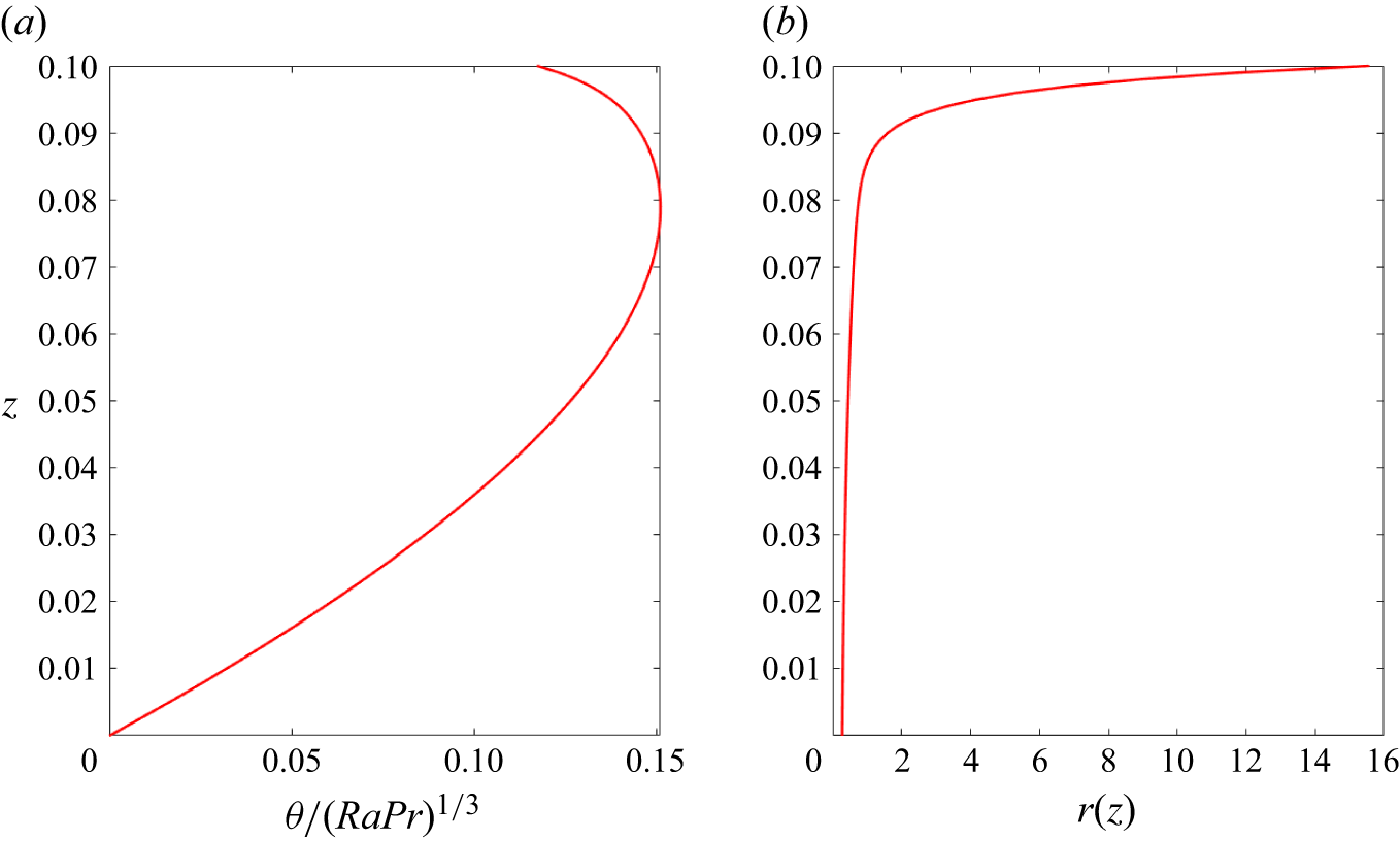
 θ
 Ra
 Pr
 r
 Bi=1.4
 f=0.5
 km=[0.018,0.325,2.75,30]
 ζb≈0.4178
 Pm/ζbkm=[63.9594,1.4287,0.1071,0.0161]
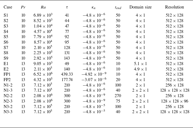
 tend
 Ra
 Ra=τ3/Pr
 τ
 Pr
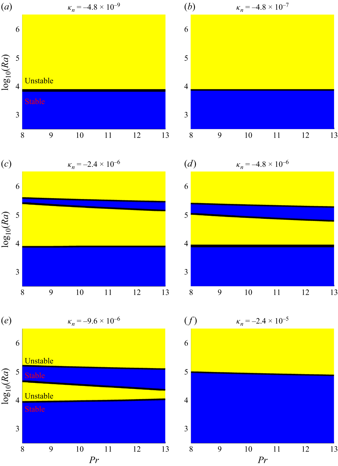
 κn
 Ra
 α
 Ra
 κn
 Q0
 α
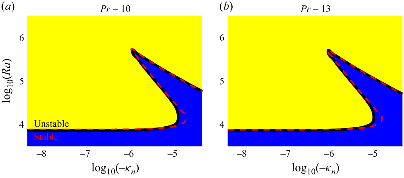
 κn
 Ra
 Pr=10
 Pr=13
 Ra
 κn
 Pr
 Ra
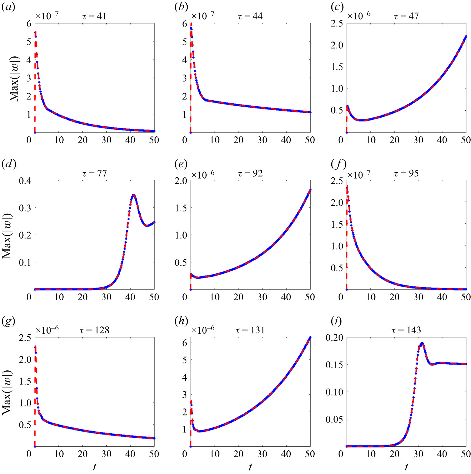
 |w|
 t
 κn=−4.8×10⁻⁶
 Pr=10
 τ=(RaPr)1/3
 |w|
 τ
 τc=43.07,93.38
 128.53
 Rac=
 7.99×10³
 8.14×10⁴
 2.12×10⁵
 t=50
 τ=77
 τ=143
 t=50

 Pr=13
 κn=−4.8×10⁻⁶
 Ra=2.11×10⁵
 τ=140
 κn=−4.8×10⁻⁶
 Ra=9.05×10³
 τ=49
 Ra
 Ra
 ρb/ρ0−1
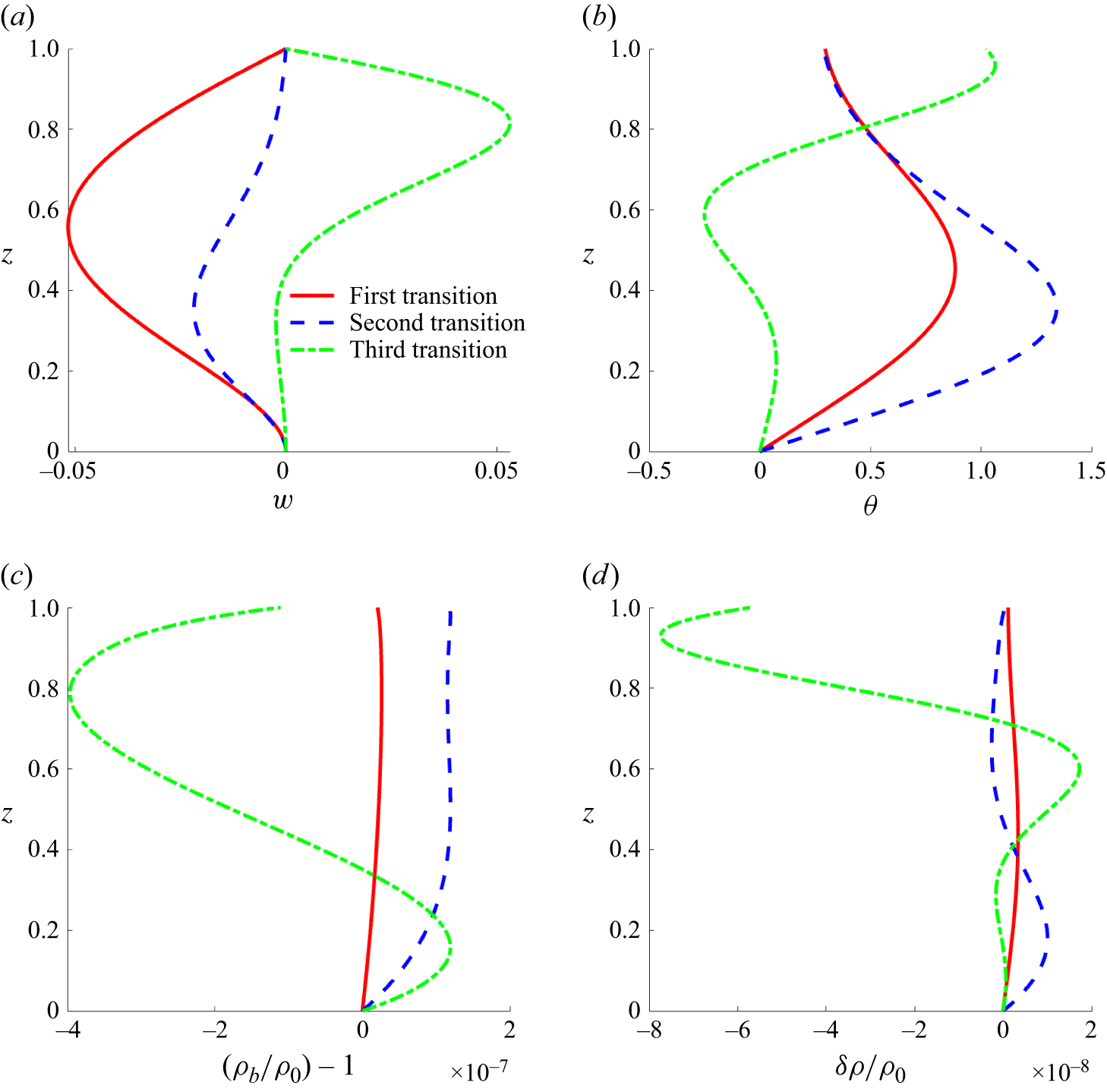
 κn=−4.8×10⁻⁶
 Pr=10
 w
 θ
 ρb/ρ0−1
 ρb
 δρ/ρ0
 δρ
 τ=(RaPr)1/3
 IN/I1=0.0422,0.0349
 0.1673

 w
 θ
 κn=−4.8×10⁻⁹,Pr=13
 κn=−4.8×10⁻⁵,Pr=13
 IN/I1=0.0402,0.1121
 |κn|
 |κn|

 κn=−4.92×10⁻⁹,Ra=6.52×10⁶
 τ=(RaPr)1/3=439.33
 θ0+θ

 κn=−3.07×10⁻⁶,Ra=4.32×10⁵
 τ=177.74
 θ0+θ

 t≈40
 t≈100
 κn=−4.8×10⁻⁶,Ra=7.12×10⁵
 τ=(RaPr)1/3=210
 tend
 Δt=0.5
 t

 tend
 t≈40
 t≈100
 κn=−4.8×10⁻⁵,Ra=7.12×10⁵
 τ=210
 t≈40

 tend
 t≈75
 t≈270
 κn=−4.8×10−9,2.08×106
 τ=300

 κn
 SA
 T0
 κn

 Q0
 SA
 Q0
 SA
 SA
 Q0
 t=50
 Δt=0.5
 tend
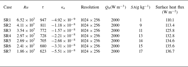
 Q0=2000Wm−3
 4×1
 Pr=13
 tend=50
 Δt=0.5
 tend

 Ra
 Bi
 Pr=10
 κn=−4.8×10⁻⁶

 Open access

