2 Derivation of the stability equation

In this section we first provide details of the contour-dynamics formulation in the 3D axisymmetric geometry, which is the basis of our approach. Then, methods of the shape calculus are used to derive an integro-differential equation characterizing the stability of Hill’s vortex. Finally, we discuss some properties of this equation. Hereafter $\mathscr{A}$ will denote the projection of the axisymmetric vortex region $\mathscr{D}$ onto the meridional plane $\{x,{\it\sigma}\}$ .

The formalism of contour dynamics is a convenient way to study the evolution of inviscid flows with piecewise smooth vorticity distributions (Pullin Reference Pullin1992). Given a time-dependent region $\mathscr{A}(t)$ , where $t$ is time, its evolution can be studied by tracking the points $\boldsymbol{y}(t)$ on its boundary $\partial \mathscr{A}(t)$ via the equation

where $\unicode[STIX]{x1D646}(\boldsymbol{y}(t),\boldsymbol{y}^{\prime })$ is a suitable Biot–Savart kernel, $\boldsymbol{y}$ and $\boldsymbol{y}^{\prime }$ are defined in the absolute frame of reference and $\text{d}s_{\boldsymbol{y}^{\prime }}$ is an arclength element of the vortex boundary in the meridional plane. An equilibrium shape of the vortex boundary, denoted $\partial \mathscr{A}$ (without the argument $t$ ), can be characterized by transforming the coordinates to the translating frame of reference $\boldsymbol{x}(t):=\boldsymbol{y}(t)-Wt\,\boldsymbol{e}_{x}$ and considering the normal component of (2.1),

where $\boldsymbol{n}_{\boldsymbol{x}}$ denotes the unit vector normal to the contour $\partial \mathscr{A}$ at the point $\boldsymbol{x}$ (hereafter we will use the convention that a subscript on a geometric quantity will indicate where this quantity is evaluated). Since we have $\boldsymbol{x}(0)=\boldsymbol{y}(0)$ , the arguments of the kernel $\unicode[STIX]{x1D646}$ in (2.2) can be changed to $\boldsymbol{x}$ and $\boldsymbol{x}^{\prime }$ . Equation (2.2) expresses the vanishing of the normal velocity component on the vortex boundary in relative equilibrium. Since the equilibrium shape of the boundary $\partial \mathscr{A}$ is in general a priori unknown, relation (2.2) reveals the free-boundary aspect of the problem. The Biot–Savart kernel was derived by Wakelin & Riley (Reference Wakelin and Riley1996) with an alternative, but equivalent, formulation also given by Pozrikidis (Reference Pozrikidis1986). Here we will use this kernel in the form rederived and tested by Shariff, Leonard & Ferziger (Reference Shariff, Leonard and Ferziger2008),

where

in which

whereas ${\it\theta}^{\prime }$ denotes the polar angle of the point $\boldsymbol{x}^{\prime }$ , i.e. $\cos {\it\theta}^{\prime }=x^{\prime }/\sqrt{x^{\prime 2}+{\it\sigma}^{\prime 2}}$ and $\sin {\it\theta}^{\prime }={\it\sigma}^{\prime }/\sqrt{x^{\prime 2}+{\it\sigma}^{\prime 2}}$ , and $K(\tilde{r})$ and $E(\tilde{r})$ are the complete elliptic integrals of the first and second kind, respectively (Olver et al. Reference Olver, Lozier, Boisvert and Clark2010). We note that $\tilde{r}\rightarrow 1$ as $x^{\prime }\rightarrow x$ and ${\it\sigma}^{\prime }\rightarrow {\it\sigma}$ , and at $\tilde{r}=1$ function $K(\tilde{r})$ has a logarithmic singularity (more details about the singularity structure of kernel (2.3) will be provided below).

In addition to the circulation, impulse and energy conserved by all classical solutions of Euler’s equations, axisymmetric inviscid flows also conserve Casimirs $\iint _{\mathscr{A}(t)}{\it\Phi}({\it\omega}/{\it\sigma})\,{\it\sigma}\,\text{d}\mathscr{A}$ , where ${\it\Phi}:\mathbb{R}\rightarrow \mathbb{R}$ is an arbitrary function with sufficient regularity (Mohseni Reference Mohseni2001). Since circulation is particularly important from the physical point of view, we will focus on stability analysis with respect to perturbations preserving this quantity, which is the same approach as was also taken by Moffatt & Moore (Reference Moffatt and Moore1978). Circulation ${\it\Gamma}$ of the flow in the meridional plane is defined as

and can also be viewed as the Casimir corresponding to ${\it\Phi}({\it\xi})={\it\xi}$ . We add that, since the flows considered here have the property ${\it\omega}=\mathscr{C}{\it\sigma}$ , cf. (1.1)–(1.2), conservation of circulation (2.7) implies the conservation of the volume of the vortical region.

Following the ideas laid out by Elcrat & Protas (Reference Elcrat and Protas2013), we introduce a parametrization of the contour $\boldsymbol{x}=\boldsymbol{x}(t,s)\in \partial \mathscr{A}(t)$ in terms of its arclength $s$ . We will also adopt the convention that the superscript ${\it\epsilon}$ , where $0<{\it\epsilon}\ll 1$ , will denote quantities corresponding to the perturbed boundary, so that $\boldsymbol{x}=\boldsymbol{x}^{{\it\epsilon}}|_{{\it\epsilon}=0}$ and $\boldsymbol{n}_{\boldsymbol{x}}=\boldsymbol{n}_{\boldsymbol{x}^{{\it\epsilon}}}|_{{\it\epsilon}=0}$ are the quantities corresponding to the (relative) equilibrium. Then, points on the perturbed vortex boundary can be represented as

where $r(t,s)$ represents the ‘shape’ of the perturbation. We note that, without affecting the final result, $\boldsymbol{n}_{\boldsymbol{x}}(s)$ in the last term in (2.8) could be replaced by its perturbed counterpart, $\boldsymbol{n}_{\boldsymbol{x}^{{\it\epsilon}}}(t,s)$ . Using (2.1) we thus deduce

from which the equilibrium condition (2.2) is obtained by setting ${\it\epsilon}=0$ . The perturbation equation is obtained by linearizing relation (2.9) around the equilibrium configuration characterized by (2.2), which is equivalent to expanding (2.9) in powers of ${\it\epsilon}$ and retaining the first-order terms. Since (2.9) involves perturbed quantities defined on the perturbed vortex boundary $\partial \mathscr{A}^{{\it\epsilon}}(t)$ , the proper way to obtain this linearization is using methods of the shape-differential calculus (Delfour & Zolésio Reference Delfour and Zolésio2001). Below we state the main results only and refer the reader to our earlier study (Elcrat & Protas Reference Elcrat and Protas2013) for details of all intermediate transformations. Shape-differentiating the left-hand side (LHS) of relation (2.9) and setting ${\it\epsilon}=0$ we obtain

As regards the right-hand side (RHS) in (2.9), we obtain

where $\boldsymbol{t}_{\boldsymbol{x}}$ is the unit tangent vector and ${\it\varkappa}_{\boldsymbol{x}}$ the curvature of the contour $\partial \mathscr{A}$ (in the present case, with the contour $\partial \mathscr{A}$ given by a half-circle of unit radius, ${\it\varkappa}\equiv 1$ ). The orientation of the unit vectors $\boldsymbol{t}_{\boldsymbol{x}}$ and $\boldsymbol{n}_{\boldsymbol{x}}$ and the sign of the curvature ${\it\varkappa}_{\boldsymbol{x}}$ satisfy Frenet’s convention. As explained by Elcrat & Protas (Reference Elcrat and Protas2013), the three terms on the RHS of (2.11) represent the shape-sensitivity of the RHS of (2.9) to perturbations (2.8) applied separately to the normal vector $\boldsymbol{n}_{\boldsymbol{x}}$ , the evaluation point $\boldsymbol{x}$ and the contour $\partial \mathscr{A}$ over which the integral is defined. Since the flow evolution is subject to constraint (2.7), this will restrict the admissible perturbations $r$ . Indeed, noting that ${\it\omega}=\mathscr{C}{\it\sigma}$ , cf. (1.1)–(1.2), and shape-differentiating relation (2.7), we obtain the following condition (Elcrat & Protas Reference Elcrat and Protas2013):

restricting the class of admissible perturbations to those which do not modify the circulation (2.7), although the vorticity may change locally (analogous conditions can be obtained when the perturbations are constructed to preserve other integral invariants mentioned above). In the case of Hill’s vortex with the assumed parameter values, the equilibrium shape of the vortex boundary is given by the sphere of unit radius, so that $\partial \mathscr{A}=\{(x,{\it\sigma})\;:\;x^{2}+{\it\sigma}^{2}=1\}$ . In such a case, the arclength coordinate $s$ can be identified with the polar angle ${\it\theta}\in [0,{\rm\pi}]$ , so that $x=\cos {\it\theta}$ and ${\it\sigma}=\sin {\it\theta}$ . Therefore, below, we will use ${\it\theta}$ as our independent variable.

Combining (2.10)–(2.12) and replacing the line integrals with the corresponding definite ones, we finally obtain the perturbation equation

where $\mathscr{L}$ denotes the associated linear operator and in which

As regards the singularities of the kernels, one can verify by inspection that

The singularities of the kernels $I_{1}({\it\theta},{\it\theta}^{\prime })$ and $I_{2}({\it\theta},{\it\theta}^{\prime })$ vanish at ${\it\theta}=0$ and ${\it\theta}={\rm\pi}$ . Properties (2.17a )–(2.17d ) will be instrumental in achieving spectral accuracy in the discretization of system (2.13).

Equation (2.13a ) is a first-order integro-differential equation and as such would in principle require only one boundary condition. However, since the kernel (2.3) is obtained via averaging with respect to the azimuthal angle ${\it\phi}$ (due to the axisymmetry assumption (see Shariff et al. Reference Shariff, Leonard and Ferziger2008)), the different terms and integrands in (2.13a ) exhibit the following reflection symmetries:

indicating that (2.13a ) is invariant with respect to the change of the independent variable ${\it\eta}=-{\it\theta}\in [-{\rm\pi},0]$ . This means that when (2.13a ) is considered on an extended periodic domain $[-{\rm\pi},{\rm\pi}]$ subject to even initial data $r(0,{\it\theta})=r(0,-{\it\theta})$ , ${\it\theta}\in (0,{\rm\pi})$ , its solution will also remain an even function of ${\it\theta}$ at all times, i.e. $r(t,{\it\theta})=r(t,-{\it\theta})$ , $t>0$ . In particular, if they are smooth enough, these solutions will satisfy the symmetry conditions

Thus, system (2.13) with even initial data (which is consistent with the axisymmetry assumption) and subject to boundary conditions (2.19) is not an over-determined problem. These observations will be used in the next section to construct a spectral discretization of (2.13a ).

After introducing the ansatz

where $\text{i}:=\sqrt{-1}$ and ${\it\lambda}\in \mathbb{C}$ , system (2.13) together with the boundary conditions (2.19) takes the form of a constrained eigenvalue problem:

where the operator $\mathscr{L}$ is defined in (2.13a ). The eigenvalues ${\it\lambda}$ and the eigenfunctions $u$ characterize the stability of Hill’s vortex to axisymmetric perturbations.

3 Numerical approach

In this section we describe the numerical approach with a focus on the discretization of system (2.21) and the solution of the resulting algebraic eigenvalue problem. We will also provide some details about how this approach has been validated. We are interested in achieving the highest possible accuracy and, in principle, eigenvalue problems for operators defined in the continuous setting on one-dimensional (1D) domains can be solved with machine precision using chebfun (Driscoll, Hale & Trefethen Reference Driscoll, Hale and Trefethen2014). However, at present, chebfun does not have the capability to deal with singular integral operators such as $\mathscr{L}$ . We have therefore implemented an alternative hybrid approach relying on a representation of the operator $\mathscr{L}$ in a trigonometric basis in which kernel singularities are treated analytically and chebfun is used to evaluate the remaining definite integrals with high precision.

The eigenfunctions $u$ are approximated with the truncated series

where ${\it\alpha}_{0},\ldots ,{\it\alpha}_{N-1}\in \mathbb{R}$ are unknown coefficients, which satisfies exactly the boundary conditions (2.19). The interval $[0,{\rm\pi}]$ is discretized with equispaced grid points,

(both endpoints are included in the grid). After substitution of ansatz (3.1), equation (2.21a ) is collocated on grid (3.2), whereas constraint (2.21c ) takes the form

in which the integrals are evaluated as

(we note that these integrals vanish for all odd values of $k$ ). As a result, we obtain the following discrete eigenvalue problem:

in which

is the (invertible) collocation matrix, whereas the matrices $\unicode[STIX]{x1D63D}$ , $\unicode[STIX]{x1D63E}$ and $\unicode[STIX]{x1D63F}$ correspond to the three terms in operator $\mathscr{L}$ , cf. (2.13a ). We remark that the terms corresponding to all values $k=0,\ldots ,N-1$ have to be included in expansion (3.1), even though their sum might not satisfy constraint (2.13b ), as otherwise the collocation problem is not well posed (i.e. matrix (3.6) is singular). Constraint (2.12) is then imposed through the generalized formulation (3.5).

The entries of matrix $\unicode[STIX]{x1D63D}$ , corresponding to the first term in operator $\mathscr{L}$ , are defined as follows:

The entries of matrix $\unicode[STIX]{x1D63E}$ , corresponding to the second term in operator $\mathscr{L}$ , are defined as follows:

where the coefficient is given by an improper integral evaluated using the property (2.17d ) to separate the singular part of the kernel (Hackbusch Reference Hackbusch1995)

Here $\mathscr{T}({\it\theta})$ has a bounded and continuous integrand expression and can therefore be accurately evaluated using the function sum from chebfun (for ${\it\theta}^{\prime }\approx {\it\theta}$ the integrand is represented in terms of a generalized series expansion), whereas $\mathscr{S}({\it\theta})$ can be computed analytically as

The entries of matrix $\unicode[STIX]{x1D63F}$ , corresponding to the last term in operator $\mathscr{L}$ , are defined as follows:

which represents the action of a weakly singular integral operator on trigonometric functions. In the light of the property (2.17c ), they are evaluated similarly to (3.9) by separating the singular part of the kernel. We thus obtain

Here $\mathscr{T}_{k}({\it\theta})$ has a bounded and continuous integrand expression and can therefore be accurately evaluated using the function sum from chebfun (for ${\it\theta}^{\prime }\approx {\it\theta}$ the integrand is represented in terms of a generalized series expansion). As regards $\mathscr{S}_{k}({\it\theta})$ , for $k=0$ , it is already given in (3.10). For $k>0$ , we obtain

where $\mathscr{E}_{1}(z)$ , $z\in \mathbb{C}$ , is the exponential integral defined as the complex extension of the function $\mathscr{E}_{1}(x):=\int _{x}^{\infty }(\text{e}^{-t}/t)\,\text{d}t$ , $x>0$ (Olver et al. Reference Olver, Lozier, Boisvert and Clark2010). We note that, while the LHS of relation (3.13) is real-valued, it is evaluated in terms of a combination of complex-valued expressions. Since the exponential integral is multi-valued in the complex plane, care must be taken that its values used in (3.13) are taken from the same sheath.

The eigenvalue problem (3.5a ) needs to be restricted to eigenfunctions satisfying condition (3.5b ) and this is done with a projection approach. Defining $\boldsymbol{u}=[{\it\alpha}_{0},\ldots ,{\it\alpha}_{N-1}]^{\text{T}}$ and the matrix $\unicode[STIX]{x1D648}:=-\text{i}\,\unicode[STIX]{x1D63C}^{-1}(\unicode[STIX]{x1D63D}+\unicode[STIX]{x1D63E}+\unicode[STIX]{x1D63F})$ , equation (3.5a ) can be expressed as

Introducing operator $\boldsymbol{b}:\mathbb{R}^{N}\longrightarrow \mathbb{R}$ defined as

the constraint (3.5b ) can be expressed as $\boldsymbol{b}\boldsymbol{u}=0$ . The kernel space of this operator, $\mathscr{N}(\boldsymbol{b})$ , thus corresponds to the subspace of functions satisfying condition (3.5b ). The projection onto this subspace is realized by the operator $\mathscr{P}_{\!\!\mathscr{N}(\boldsymbol{b})}:=\unicode[STIX]{x1D644}-\boldsymbol{b}^{\dagger }\boldsymbol{b}$ , where $\unicode[STIX]{x1D644}$ is the $N\times N$ identity matrix and $\boldsymbol{b}^{\dagger }:=\boldsymbol{b}^{\text{T}}(\boldsymbol{b}\boldsymbol{b}^{\text{T}})^{-1}=\boldsymbol{b}^{\text{T}}/\Vert \boldsymbol{b}\Vert _{2}$ is the Moore–Penrose pseudo-inverse of the operator $\boldsymbol{b}$ (Laub Reference Laub2005). Defining the restricted variable $\boldsymbol{z}:=\mathscr{P}_{\!\!\mathscr{N}(\boldsymbol{b})}\,\boldsymbol{u}$ , problem (3.14) transforms to

where $\mathscr{P}_{\!\!\mathscr{N}(\boldsymbol{b})}^{\dagger }$ is the Moore–Penrose pseudo-inverse of the projector $\mathscr{P}_{\!\!\mathscr{N}(\boldsymbol{b})}$ , which can now be solved using standard techniques. We note that the dimension of this problem is $N-1$ . An alternative approach to impose constraint (3.5b ) is to frame (3.5) as a generalized eigenvalue problem (Laub Reference Laub2005).

We now offer some comments about the accuracy and validation of the computational approach described above. The accuracy of approximation of singular integrals in (3.9) and (3.12) was tested by applying this approach to the integral operator in (2.2), which has the same singularity structure as $\mathscr{T}({\it\theta})$ in (3.9) and $\mathscr{T}_{k}({\it\theta})$ in (3.12), and for which an exact formula is available, cf. (1.3). In addition, an analogous test was conducted for the tangential velocity component given by $\mathscr{C}\,\boldsymbol{t}_{{\it\theta}}\boldsymbol{\cdot }[\int _{0}^{{\rm\pi}}\unicode[STIX]{x1D646}({\it\theta},{\it\theta}^{\prime })\,\text{d}{\it\theta}^{\prime }-W\,\boldsymbol{e}_{x}]$ . Using $\mathtt{maxLength}=10^{6}$ (which controls the length of the Chebyshev series in chebfun) resulted in $L_{\infty }$ errors of order $\mathit{O}(10^{-12})$ , which is close to the machine precision. The rather complicated analytical expression (3.13) used in $\mathscr{S}_{k}({\it\theta})$ , involving multi-valued functions with branch cuts in the complex plane, was validated by comparing it against a numerical approximation of the weakly singular integral defining $\mathscr{S}_{k}({\it\theta})$ . With the high precision of the numerical quadratures thus verified, the shape differentiation results in (2.11) were validated by comparing them against simple forward finite-difference approximations of the shape derivatives. For example, the consistency of the first term on the RHS in (2.11) was checked by comparing it (as a function of ${\it\theta}$ ) to

in the limit of vanishing ${\it\epsilon}$ . In the same spirit, the consistency of the second and third terms on the RHS of (2.11) was verified by perturbing the evaluation point $\boldsymbol{x}$ and the contour $\partial \mathscr{A}$ , respectively. We also checked computationally that the projection formulation (3.16) of the constrained eigenvalue problem (2.21) gives essentially the same results as its formulation in terms of a generalized eigenvalue problem (the former approach was in fact found to be somewhat more sensitive to round-off errors owing to the conditioning of the projection operator $\mathscr{P}_{\!\!\mathscr{N}(\boldsymbol{b})}$ ). The algebraic eigenvalue problem was solved in Matlab with the QR and Cholesky methods producing essentially identical results.

Anticipating the results of § 4, we now introduce a regularized version of eigenvalue problem (3.16) in which it is ensured that the coefficients ${\it\alpha}_{k}$ decay with the wavenumber $k$ sufficiently rapidly, thus guaranteeing the required regularity of the eigenvectors $\boldsymbol{u}$ . We introduce the following diagonal operator acting as a low-pass filter:

where ${\it\delta}>0$ is the cut-off length scale and $p$ a positive integer, and define $\boldsymbol{z}^{{\it\delta}}:=\unicode[STIX]{x1D641}^{{\it\delta}}\,\boldsymbol{z}$ . This filter can be regarded as the discretization of the elliptic operator $[\text{Id}-(-1)^{p+1}{\it\delta}^{2p}\,\partial ^{2p}/\partial {\it\theta}^{2p}]^{-1}$ in the trigonometric basis. We then obtain from (3.16)

from which the original problem is clearly recovered when ${\it\delta}\rightarrow 0$ . The regularized eigenvectors $\boldsymbol{u}^{{\it\delta}}$ corresponding to $\boldsymbol{z}^{{\it\delta}}$ are therefore guaranteed to be smoother than the original eigenvectors $\boldsymbol{u}$ (the actual improvement of smoothness depends on the value of $p$ ). In the next section, among other results, we will study the behaviour of solutions to eigenvalue problem (3.19) for a decreasing sequence of regularization parameters  ${\it\delta}$ .

Figure 1.

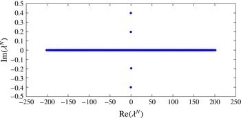
Eigenvalue spectrum of problem (3.19) obtained with $N=1024$ and ${\it\delta}=1/32$ .

4 Computational results

In this section we first summarize the numerical parameters used in the computations and then present the results obtained by solving eigenvalue problem (3.19) for different values of the regularization parameter ${\it\delta}$ . All computations were conducted setting $p=4$ in the regularization operator (3.18) and using the resolutions $N=64,128,256,512,1024$ in (3.1). We allowed the regularization parameter to take a wide range of values ${\it\delta}=1,1/2,1/4,\ldots ,1/1024$ . We note that, with the smallest values from this range, regularization barely affects the eigenvalue problem (3.19) even when the highest resolutions are used. Therefore, these values may be considered small enough to effectively correspond to the limit ${\it\delta}\rightarrow 0$ .

In our analysis below we will first demonstrate that, for a fixed parameter ${\it\delta}$ , the solutions of the regularized problem (3.19) converge as the numerical resolution $N$ is refined. Then, we will study the behaviour of the eigenvalues and eigenfunctions as the regularization parameter ${\it\delta}$ is reduced. A typical eigenvalue spectrum obtained by solving problem (3.19) is shown in figure 1. The fact that the spectrum is symmetric with respect to the lines $\text{Re}({\it\lambda})=0$ and $\text{Im}({\it\lambda})=0$ reflects the Hamiltonian structure of the problem. Given the ansatz for the perturbations introduced in § 2, eigenvalues with negative imaginary parts correspond to linearly unstable eigenmodes, and we see in figure 1 that there are two such eigenvalues in addition to two eigenvalues associated with linearly stable eigenmodes. We will refer to the eigenvalues with the larger and the smaller magnitudes as the first and the second, respectively. In addition to these four purely imaginary eigenvalues, there is also a large number of purely real eigenvalues covering a segment of the axis $\text{Im}({\it\lambda})=0$ , which can be interpreted as the continuous spectrum. The spectrum shown in figure 1 was found to be essentially independent of the regularization parameter ${\it\delta}$ , and its dependence on the numerical resolution $N$ is discussed below. In this analysis we will set ${\it\delta}=1/32$ .

Figure 2.

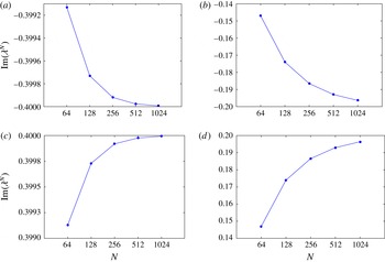
Dependence of the four purely imaginary eigenvalues on the resolution $N$ with a fixed regularization parameter ${\it\delta}=1/32$ . The eigenvalues shown in (a) and (b) correspond to the two unstable eigenmodes, whereas those shown in (c) and (d) correspond to the two stable eigenmodes.

The dependence of the four purely imaginary eigenvalues on the resolution $N$ is shown in figure 2(a–d), where we see that the eigenvalues all converge to well-defined limits. However, as will be discussed below, problem (3.5) does not admit smooth solutions (eigenvectors) and therefore the convergence of eigenvalues ${\it\lambda}^{N}$ with $N$ is only algebraic rather than spectral. Thus, the numerical approximation error for an eigenvalue ${\it\lambda}$ can be represented as $|{\it\lambda}^{N}-{\it\lambda}|=cN^{{\it\beta}}$ for some $c>0$ and ${\it\beta}<0$ . 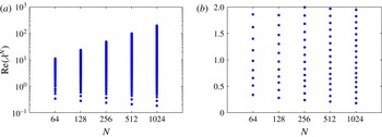Using the data from figure 2 to evaluate $({\it\lambda}^{N}-{\it\lambda}^{2N})$ as a function of the resolution $N$ , one can estimate the order of convergence using a least-squares fit as ${\it\beta}\approx -1.72$ for the first eigenvalue (both stable and unstable) and ${\it\beta}\approx -0.99$ for the second (both stable and unstable). This confirms that the first eigenvalues converge much faster than the second. The dependence of the purely real eigenvalues on the resolution $N$ is illustrated in figure 3(a,b). First of all, we notice that the purely real eigenvalues do not appear to converge to any particular limit as $N$ is increased and instead fill an interval of the axis $\text{Im}({\it\lambda})=0$ with increasing density (figure 3 b). From figure 3(a) we can infer that the lower and upper bounds of this interval approximately scale with the resolution as

where ${\it\lambda}_{i}^{N}$ denotes the $i$ th eigenvalue computed with the resolution $N$ . All these observations allow us to conclude that the continuous eigenvalue problem (2.21) has four purely imaginary eigenvalues and a continuous spectrum coinciding with the axis $\text{Im}({\it\lambda})=0$ .

Figure 3.

Dependence of the purely real eigenvalues on the resolution $N$ with a fixed regularization parameter ${\it\delta}=1/32$ plotted (a) using the logarithmic scale and (b) within the interval $[0,2]$ using the linear scale for the vertical axis. For clarity, only the eigenvalues with positive real parts ( $\text{Re}({\it\lambda}_{i}^{N})>0$ ) are shown.

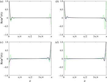
We now move on to discuss the eigenvectors corresponding to the purely imaginary eigenvalues. The linearly unstable and stable eigenvectors are shown as functions of the polar angle ${\it\theta}$ for different resolutions $N$ in figure 4(a–d). In this figure we only show the real parts of the eigenvectors, since, given our ansatz (2.20) for the perturbation, the imaginary parts do not play any role when the eigenvalues are purely imaginary. Hence, below, the term ‘eigenvector’ will refer to $\text{Re}(\boldsymbol{u}^{N}({\it\theta}))$ . We note that, as the resolution $N$ increases, the unstable and stable eigenvectors associated with a given eigenvalue become reflections of each other with respect to the midpoint ${\it\theta}={\rm\pi}/2$ , with the unstable eigenvectors exhibiting a localized peak near the rear stagnation point ( ${\it\theta}=0$ ) and the stable eigenvectors exhibiting such a peak near the front stagnation point ( ${\it\theta}={\rm\pi}$ ). In figure 4(a–d) we also observe that, for a fixed regularization parameter ${\it\delta}$ , the numerical approximations $\text{Re}(\boldsymbol{u}^{N}({\it\theta}))$ of eigenfunctions converge uniformly in ${\it\theta}$ for increasing $N$ , although this convergence is significantly slower for points ${\it\theta}$ close to the endpoint opposite to where the eigenvector exhibits a peak. We remark that the same behaviour of spectral approximations to eigenfunctions was also observed by Rozi (Reference Rozi1999). The two unstable eigenvectors $\text{Re}(\boldsymbol{u}_{1}^{N})$ and $\text{Re}(\boldsymbol{u}_{2}^{N})$ are strongly non-normal, with $\langle \,\text{Re}(\boldsymbol{u}_{1}^{N}),\text{Re}(\boldsymbol{u}_{2}^{N})\,\rangle _{L_{2}}/(\Vert \text{Re}(\boldsymbol{u}_{1}^{N})\Vert _{L_{2}}\Vert \text{Re}(\boldsymbol{u}_{2}^{N})\Vert _{L_{2}})\approx 0.96$ , where $\langle \cdot ,\cdot \rangle _{L_{2}}$ and $\Vert \cdot \Vert _{L_{2}}$ are, respectively, the inner product and the norm in the space $L_{2}(0,{\rm\pi})$ , when ${\it\delta}=1/32$ and $N=1024$ . Consequently, the two unstable eigenvectors appear quite similar as functions of ${\it\theta}$ , especially near the peak (cf. 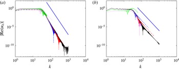figure 4 a,b). On the other hand, the Fourier spectra of their expansion coefficients shown in figure 5(a,b) exhibit quite distinct properties. More specifically, we see that the slope of the Fourier spectra for $k>1/{\it\delta}$ is quite different in the two cases: it is close to $-7$ and $-5$ for the eigenvectors associated with, respectively, the first and second eigenvalue. 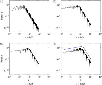We emphasize however that the specific slopes are determined by the choice of the parameter $p$ in the regularizing operator (3.18) and here we are interested in the relative difference of the slopes in the two cases. Further distinctions between the eigenvectors associated with the first and the second eigenvalue will be elucidated below when discussing their behaviour in the limit of decreasing regularization parameter  ${\it\delta}$ .

Figure 4.

Unstable eigenvectors corresponding to the first (a) and second (b) eigenvalue, and stable eigenvectors corresponding to the first (c) and second (d) eigenvalue for different resolutions: $N=64$ (green solid line), $N=128$ (magenta dotted line), $N=256$ (blue dash-dotted line), $N=512$ (red dashed line) and $N=1024$ (thick black solid line) with ${\it\delta}=1/32$ . The eigenvectors are normalized such that $\sup _{{\it\theta}\in [0,{\rm\pi}]}|\text{Re}(\boldsymbol{u}^{N}({\it\theta}))|=1$ .

Figure 5.

Fourier coefficient spectra $|\text{Re}({\it\alpha}_{k})|$ , $k=1,\ldots ,N$ , characterizing the eigenvectors associated with the first (a) and the second (b) eigenvalue for different resolutions: $N=64$ (green solid line), $N=128$ (magenta dotted line), $N=256$ (blue dash-dotted line), $N=512$ (red dashed line) and $N=1024$ (thick black solid line). The spectra of the stable and unstable eigenvectors corresponding to eigenvalues with the same magnitude are identical. The straight blue solid lines show the slopes of $-7$  (a) and  $-5$  (b).

Figure 6.

Dependence of the unstable eigenvectors associated with the first (black solid line) and the second (red dashed line) eigenvalue on the polar angle ${\it\theta}$ near the rear (a) and the front (b) stagnation point for different values of the regularization parameter ${\it\delta}=1/32,1/64,1/96,1/128$ with $N=1024$ (smaller values of ${\it\delta}$ correspond to more localized eigenvectors). The eigenvectors are normalized such that $\sup _{{\it\theta}\in [0,{\rm\pi}]}|\text{Re}(\boldsymbol{u}^{N}({\it\theta}))|=1$ .

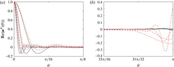
Having established the convergence of the numerical approximations of the eigenfunctions with the resolution $N$ for a fixed regularization parameter ${\it\delta}$ , we now go on to characterize their behaviour when ${\it\delta}$ is decreased. Unless indicated otherwise, the results presented below were obtained with the resolution $N=1024$ . In figure 6(a,b) we show the behaviour of the two unstable eigenvectors near the rear and front stagnation points for different values of the regularization parameter ${\it\delta}$ . We see that, as this parameter is decreased, the peak near the rear stagnation point (figure 6 a) becomes steeper and more localized, especially for the eigenvector associated with the first eigenvalue. 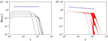Likewise, the oscillation of the unstable eigenvectors near the front stagnation point (figure 6 b) also becomes more intense and localized as ${\it\delta}$ decreases, although this effect is more pronounced in the case of the eigenvector corresponding to the second eigenvalue. These properties are further characterized in the plots of the Fourier spectra of the two eigenvectors shown in figure 7(a,b) for different values of the regularization parameter ${\it\delta}$ . In these plots it is clear that, as the regularization effect vanishes (corresponding to decreasing values of ${\it\delta}$ ), the point where the slope of the spectrum changes moves towards larger wavenumbers $k$ . For $k<1/{\it\delta}$ the approximate slopes of the coefficient spectra are, respectively, $0$ and $-1/8$ for the eigenvectors associated with the first and second eigenvalue (this difference of slopes may explain the different behaviours in the physical space already observed in figure 6(b)). Extrapolating from the trends evident in figure 7(a,b) it can be expected that these slopes will remain unchanged in the limit ${\it\delta}\rightarrow 0$ . With this behaviour of the Fourier coefficients, involving no decay at all for the first eigenvector and a slow decay for the second, expansion (3.1) does not converge in the limit of $N\rightarrow \infty$ , indicating that the stable and unstable eigenvectors do not have the form of smooth functions, but rather are ‘distributions’. As regards the nature of their singularity, the slopes observed in figure 7(a,b), i.e. $0$ and $-1/8$ , indicate that the eigenvector associated with the first eigenvalue is consistent with the Dirac delta (whose spectral slope is also 0), whereas the eigenvector associated with the second eigenvalue is intermediate between the Dirac delta and the Heaviside step function (whose spectral slope is  $-1$ ).

Figure 7.

Fourier coefficient spectra $|\text{Re}({\it\alpha}_{k})|$ , $k=1,\ldots ,N$ , of the eigenvectors associated with the first (a) and second (b) eigenvalue for different values of the regularization parameter ${\it\delta}=1/32,1/64,1/96,1/128$ with $N=1024$ (smaller values of ${\it\delta}$ correspond to the plateau in $|\text{Re}({\it\alpha}_{k})|$ extending to larger wavenumbers). The straight blue solid lines represent the slopes of $0$  (a) and $-1/8$  (b).

Finally, we go on to discuss the eigenvectors associated with the purely real eigenvalues forming the continuous part of the spectrum. Since, as demonstrated in figure 3, for increasing resolutions $N$ different eigenvalues are actually computed in the continuous spectrum, there is no sense of convergence with $N$ . We will therefore analyse here the effect of decreasing the regularization parameter ${\it\delta}$ at a fixed resolution $N=1024$ . As above, we will focus on the real parts of the eigenvectors (with the imaginary parts having similar properties). To fix attention, we consider the neutrally stable eigenvector associated with the eigenvalue ${\it\lambda}\approx 1.0502$ . 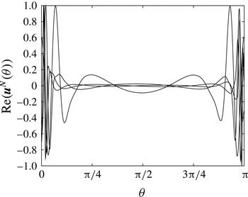In figure 8 we show the dependence of $\text{Re}(\boldsymbol{u}^{N}({\it\theta}))$ on the polar angle ${\it\theta}$ with $N=1024$ and for different values of the regularization parameter ${\it\delta}$ . We observe that, as ${\it\delta}$ decreases, the oscillations move away from the centre of the domain $[0,{\rm\pi}]$ towards the endpoints. The number of oscillations, however, remains approximately constant. The corresponding Fourier coefficient spectra are shown in figure 9(a–d). We see in these plots that the Fourier coefficients increase with $k$ as $|\text{Re}({\it\alpha}_{k})|\sim k^{3/4}$ when $k<1/{\it\delta}$ , which demonstrates that the neutrally stable eigenvectors are actually more singular objects than the stable and unstable eigenvectors discussed above. We note that, in the regularized regime (i.e. for $k>1/{\it\delta}$ ), the Fourier coefficient spectrum of the neutrally stable eigenvectors vanishes with the slope of $-7$ (see figure 9 d). Extrapolating from the trends evident in figures 8 and 9 to the limit ${\it\delta}\rightarrow 0$ , we can anticipate that the neutrally stable eigenfunctions will have the form of a finite number of oscillations localized in an infinitesimal neighbourhood of the stagnation points ${\it\theta}=0$ and ${\it\theta}={\rm\pi}$ . The number of these oscillations appears to be an increasing function of the eigenvalue magnitude  $|{\it\lambda}|$ .

Figure 8.

Real part of the neutrally stable eigenvector corresponding to the eigenvalue ${\it\lambda}\approx 1.0502$ computed with the resolution $N=1024$ and with different values of the regularization parameter ${\it\delta}=1/32,1/64,1/96,1/128$ (smaller values of ${\it\delta}$ correspond to $\text{Re}(\boldsymbol{u}^{N}({\it\theta}))$ exhibiting oscillations closer to the endpoints of the domain). The eigenvectors are normalized such that $\sup _{{\it\theta}\in [0,{\rm\pi}]}|\text{Re}(\boldsymbol{u}^{N}({\it\theta}))|=1$ .

Figure 9.

Fourier coefficient spectra $|\text{Re}({\it\alpha}_{k})|$ , $k=1,\ldots ,N$ , of the neutrally stable eigenvectors $\boldsymbol{u}^{N}$ shown in figure 8 for the indicated values of the regularization parameter ${\it\delta}$ . In (d) the blue solid lines represent the slopes of $3/4$ and $-7$ , respectively, for $k<1/{\it\delta}$ and for $k>1/{\it\delta}$ .