I. Introduction
Assessing the impact of weather on wine quality and prices has gained considerable attention. The quality of wine fundamentally depends on the quality of grapes, which is determined in part by variations in weather conditions, such as temperature and rainfall (Ashenfelter, Reference Ashenfelter2008). This recognition has led to a body of literature that examines how climate change has and may potentially affect vine yield, wine quality, and prices (Ferrise et al., Reference Ferrise, Trambi, Moriondo and Bindi2016; Jones et al., Reference Jones, White, Cooper and Storchmann2005; van Leeuwen and Darriet, Reference Ferrise, Trambi, Moriondo and Bindi2016; Webb et al., Reference Webb, Whetton and Barlow2008). The current and expected ongoing influence of climate change worldwide makes the examination of the impact of weather on wine quality and prices one of the most important and pressing issues for wine markets (Ashenfelter and Storchmann, Reference Ferrise, Trambi, Moriondo and Bindi2016).
Previous studies have examined the impact of weather on wine quality and prices at various levels and across many countries. Some studies focus on single iconic wines and examine vintage variations (Byron and Ashenfelter, Reference Byron and Ashenfelter1995); some examine a significant cross section of wines over time for a single region (Ramirez, Reference Ramirez2008); some examine the impact of weather on a particular grape variety (Haeger and Storchmann, Reference Haeger and Storchmann2006); and others have looked at the issue across countries (Jones et al., Reference Jones, White, Cooper and Storchmann2005).
This paper examines the impact of weather on the quality and prices of Australian premium wines. Significant increases in exports over the past 25 years have made Australia the fourth-largest wine exporter in the world (OIV, 2012). Australia is the largest importer to the United Kingdom (UK) (WSTA, 2012) and the third-largest importer to the United States (U.S.) market (USDA, 2012). This indicates the importance of examining the impact of weather on Australian wines. Unlike most previous price studies, ours has a wide-ranging focus and employs data from a cross section of Australian wines available in 2014. We employ a wine-quality measure from a prominent wine guide and assess the impact of weather for several wine varieties across numerous Australian wine-growing regions.
Unlike previous wine price studies, we draw on the flow of information requirements of the theoretical hedonic foundation of Rosen (Reference Rosen1974). This paper emphasizes the impact of weather on wine quality and then indirectly on price. For the general wine-buying public of retail wines, it is argued that consumers will not typically devote resources toward gaining weather-quality information about many regions and vintages to help make purchase decisions. Rather, it is argued, weather information may only possibly affect retail prices through easily accessible and publicly available wine-quality scores.
The next section provides an overview of existing literature, which supports the use of an indirect modeling approach and the weather variables employed in the model. The data set and proposed econometric model are described in section III. The results are presented and discussed in section IV, and section V is the conclusion.
II. Theoretical Considerations and Previous Literature
A significant body of literature on the hedonic pricing of wines exists; for a summary and a meta-analysis of previous studies, see Estrella Orrego et al. (Reference Estrella Orrego, De Francesco and Gennari2012) and Oczkowski and Doucouliagos (Reference Oczkowski and Doucouliagos2015). In general, these studies regress the price of wine against a series of demand and supply factors, a dominant factor being a measure of the wine's quality. An important feature of the underlying Rosen (Reference Rosen1974) hedonic theoretical foundation is that factors about which agents have knowledge are most appropriate for hedonic price models. As argued by Oczkowski (Reference Oczkowski1994) and demonstrated by Combris, Lecocq, and Visser (Reference Combris, Lecocq and Visser1997), factors relating to technical aspects, such as chemical measures (sugar, acid) and individual sensory attributes (e.g., complexity, fatness, fine tannins), may not influence prices from the demand side, as consumers have no or limited knowledge of these attributes. As a consequence, easily identifiable “objective” attributes, such as the wine's region, variety, vintage, and some publicly accessible measure of wine quality, are typically found to be the most important drivers of price variations.
The application of the perfect flow of information assumption of the Rosen (Reference Rosen1974) framework suggests that without adequate knowledge of weather variations, variables such as temperature and rainfall may not be suitable candidates for direct inclusion in hedonic price functions. It is unlikely that typical wine-buying consumers would be willing to devote resources toward identifying weather conditions of specific regions on a seasonal basis. This recognition, however, does not theoretically invalidate an examination of how weather can affect publicly available measures of wine quality and hence, indirectly, price. Even though a number of studies have examined the relation between a measure of wine quality and weather, and others have examined the direct influence of weather on price, few have examined the indirect relation of weather on price using wine quality . To facilitate the specification of the appropriate framework, we consider previous literature, which has examined the effects of weather on wine quality and prices.
A. Wine Quality and Weather
A number of studies have employed different measures of wine quality when assessing the impact of weather. Jones et al. (Reference Jones, White, Cooper and Storchmann2005) and Sadras, Soar, and Petrie (Reference Sadras, Soar and Petrie2007) employ vintage scores for various regions and their relation with temperature. Phonologically, at low temperatures, difficulties may occur in ripening grapes sufficiently for quality-wine production, and as such increasing temperature levels are expected to improve wine quality. However, in warmer regions, a quadratic relation in temperature may be important to capture the notion that, beyond an “optimal” temperature, grapes become overripe and may produce lower-quality unbalanced wines.
Jones et al. (Reference Jones, White, Cooper and Storchmann2005) examine vintage scores over a 50-year period and their relation with growing-season average temperatures and a trend variable for various countries and wine types. They find that the importance of temperature varies across countries and wine types. In general, the relation between vintage scores and temperature was stronger in Europe than in the New World. For Australian wines, the explanatory power of the trend and temperature variables in explaining vintage scores ranged between 9% and 46% and averaged 28%. In the Australian context of the six region/variety types, only white wines in the Barossa Valley had a statistically significant (10% level) quadratic relation with temperature, estimating an optimal temperature of 19.9°. Sadras, Soar, and Petrie (Reference Sadras, Soar and Petrie2007) examined vintage scores for 24 Australian regions over 25 years and found that changes in average temperature had a significant and negative impact on changes in vintage scores for red wines across regions, but an insignificant impact for white wines.
Webb et al. (Reference Webb, Whetton and Barlow2008) examined wine-grape prices as a measure of wine quality because of its relation to temperature. The examination considered 35 Australian wine regions over five vintages. Numerous weather variables were considered for analysis, and in terms of best explanatory power the mean January temperature (MJT) was chosen as the most appropriate. The R 2s for the models ranged from 0.27 to 0.83 and averaged 0.60. A significant quadratic relation between wine-grape prices and MJT was identified for four varieties, while negative and significant linear relations were identified for ten other varieties.
Finally, some studies have considered the effects of weather on quality ratings from wine guides (Cardebat et al., Reference Cardebat, Figuet and Paroissien2014; Ramirez, Reference Ramirez2008). These studies examined both temperature and rainfall variables. Rainfall near harvest time is generally considered to have a detrimental impact on wine quality as it makes harvesting difficult and increases the chances of fungal and other diseases impacting on grape quality.
Ramirez (Reference Ramirez2008) examined the impact of a trend, temperature, and rainfall on Wine Spectator quality scores for Napa Valley wines over a 35-year period. In general, only about 3% of the variation in wine quality was due to weather effects. Increasing average temperatures and higher rainfall before harvest were both associated with falling ratings, while some other temperature and rainfall variables had counterintuitive results. The quadratic form was considered inferior to a linear form.
Cardebat et al. (Reference Cardebat, Figuet and Paroissien2014) focus primarily on the impact that different expert ratings have on wine quality and prices. Wines from 11 vintages covering wineries in Bordeaux, Napa Valley, and Spain using ratings from nine experts were examined. Employing a linear specification, the average growing-season temperature is estimated to be positive and statistically significant, while the harvest rainfall is shown to be negative and significant. These findings result, irrespective of which expert rating is employed.
Both Cardebat et al. (Reference Cardebat, Figuet and Paroissien2014) and Ramirez (Reference Ramirez2008) examine the impact of weather on ratings in a single pooled analysis for wines produced from different varieties. Neither of these studies performed analyses for individual varieties and hence possibly ignore important differences due to varying growing and maturing grape variety patterns.
B. Wine Prices and Weather
The sample design for estimating the relation between weather and wines prices varies across studies. Some studies focus on a particular individual wine over its numerous vintages (Byron and Ashenfelter, Reference Byron and Ashenfelter1995; Wood and Anderson, Reference Wood and Anderson2006); others on a particular region, such as Bordeaux or Napa Valley, over numerous vintages (Ashenfelter, Reference Ashenfelter2008; Ramirez, Reference Ramirez2008); and others are predominately cross section in their focus over a region such as Médoc (Ginsburgh et al., Reference Ginsburgh, Monzak and Monzak2013) or variety such as Pinot Noir (Haeger and Storchmann, Reference Haeger and Storchmann2006).
Two Australian studies (Byron and Ashenfelter, Reference Byron and Ashenfelter1995; Wood and Anderson, Reference Wood and Anderson2006) have examined the weather effects on auction prices for single iconic wines over numerous vintages. The key employed weather variables are average growing-season temperature, the average temperature differential over the season, rain leading up to harvest, and wind. Differences in temperature over the season are expected to have a negative impact on wine quality and hence prices, as extreme variations in temperature may cause significant damage to vines and hence grape quality (Gladstones, Reference Gladstones1992). The dominant variable in these models is the age of the wine, which explains up to 60% of the price variation, with weather typically accounting for 10%–20% of total variation. For Grange, Byron and Ashenfelter (Reference Byron and Ashenfelter1995) find a quadratic relation fits the data well and identify an optimal growing-season temperature of 19°. Harvest rainfall and the temperature difference were also both found to have important negatives influences on Grange prices. Wood and Anderson (Reference Wood and Anderson2006) examined three iconic wines and found that, for growing temperature, a linear positive relation performed best for Grange and St Henri, while the quadratic fit best for Hill of Grace and an optimal temperature of 18.6°. Cubic relations for wine age and other variables such as wind, temperature difference, and harvest rain were also found to have some impact on the prices of Grange, St Henri, and Hill of Grace.
Ashenfelter (Reference Ashenfelter2008) examined Bordeaux auction prices over approximately 30 years and found that age, temperature, and rainfall explain over 80% of price variation. Unlike for the Australian iconic wines, however, weather accounts for over 60% of the variation in prices. Similarly, Ramirez (Reference Ramirez2008) examined Napa Valley prices over 35 years, explaining over 80% of the price variation using a time trend, fixed producer effects, and weather impacts. He found that 45% of the price variation is due to rain and temperature effects.
Ginsburgh, Monzak, and Monzak (Reference Ginsburgh, Monzak and Monzak2013) conducted a detailed predominately cross-section study of wines from Médoc. Price was regressed against a whole series of wine-making variables related to picking, crushing, racking, and so on; a series of weather variables including rainfall, temperature, and hail; and other variables relating to wines’ growth classification, soil, sun exposure, and so forth. The analysis revealed that climate was the second-most-important factor, after the wine's growth classification, in explaining prices .
Finally, Haeger and Storchmann (Reference Haeger and Storchmann2006) conducted a predominantly cross-section analysis of Pinot Noir prices for wines from California and Oregon. Statistically significant impacts were identified for age, production levels, growing-season temperature (quadratic), and harvest and winter rain. The addition of weather and production-level variables adds approximately 30% to the explained variation. Interestingly, the addition of quality rating points to the price equation, which examines all variables (including weather, regional and producer variables), only improves the explanatory power of the model by approximately 3%.
In summary, this review suggests that weather variables relating to growing-season temperature, seasonal temperature difference, and harvest rainfall may have an important impact on wine quality. In the relatively warmer Australian context, a negative linear or quadratic growing-season temperature relationship with wine quality is expected. It is also expected that a focus on single varieties will identify weather impacts better than an analysis that combines varieties. Further, there is a theoretical expectation that weather predominantly affects prices through accessible wine-quality ratings, rather than directly, given the high costs of attaining location- and vintage-specific weather information.
III. Data and Model
A. Data
To appropriately focus on the impact of weather on wine quality and prices, a specific sample design that examines only wines from single varieties, regions, and vintages is employed. The use of wines blended from multiple varieties and regions and across vintages potentially conflates the impact of any particular attribute, given that the proportional constituents of each blend are typically not available.
The quality rating for wines is derived from Halliday (Reference Halliday2014), whose publication is generally regarded as the most definitive, authoritative, and best selling for Australian wines. As such, Halliday (Reference Halliday2014) provides important opinion leadership in the marketplace, disseminating information about a wine's quality widely. Halliday typically tastes wines from December to March for each annual edition of his publication, and hence the wines are representative of what is currently (2014) available on the market. Prices are those listed for 2014. The use of a single year quality rating and price data source alleviates problems with inconsistency of wine evaluation over time and avoids problems in appropriately correcting price inflation effects.
From approximately 9,000 reviewed wines, the focus on wines from single varieties, regions, and vintages reduces the potential sample to 6,314 wines, made by 1,284 producers, covering 66 regions and 44 varieties (with at least 10 wines). To examine weather effects, each model focuses on a single variety, given the different growing season and maturity patterns of varieties (Dry, Reference Dry, Dry and Coombe2004). The nature of the data implies that many wines with similar weather characteristics (same region and vintage) are reviewed. This potentially limits the ability of weather characteristics to explain variations in wine quality. As a consequence, a relatively large number of sampled wines is required to identify important weather effects, typically over 150 wines for an individual variety. This requirement substantially reduces the number of varieties that can be meaningfully analyzed. Statistically significant weather effects were identified only for the eight most dominant varieties. Most of the examined wines (75% to 98% for individual varieties) came from two vintages: 2011 and 2012 for Cabernet Sauvignon, Merlot, and Shiraz; and 2012 and 2013 for Chardonnay, Pinot Noir, Riesling, Sauvignon Blanc, and Semillon.
Data for the weather variables relating to seasonal temperature and rainfall are accessed from the Australian Bureau of Meteorology (www.bom.gov.au). Weather stations most closely located to each individual winery or identified vineyard are used to generate weather information for each vintage. This was achieved by comparing the land coordinates of vineyard locations and weather stations. Even though Lecocq and Visser (Reference Lecocq and Visser2006) find that more refined weather station information for Bordeaux wines does not significantly alter the marginal weather impacts on prices, they find that information from refined stations explain an additional 7% variation in prices compared to generic Bordeaux weather locations. Similarly, for Rhine wines, Storchmann (Reference Storchmann2005) finds that the use of weather data more closely located to vineyards produces superior results. In our case, the number of weather stations per region ranges from one (for 16 regions) to seven and averages 2.8 stations per region. In cases where vineyard locations were unclear, generic region weather stations were employed. Hall and Jones (Reference Hall and Jones2009) provide evidence suggesting that available weather stations provide generally good coverage of weather conditions in the viticultural regions of Australia. In a few cases, stations were excluded as they were clearly inappropriate (e.g., being at unrepresentative extreme altitudes).
B. Econometric Model
Based on the flow of information assumption underpinning the Rosen (Reference Rosen1974) framework, we employ a two-equation recursive model. First, we estimate the relation between wine quality and weather variables and then the relation between wine prices and quality and other factors. Given the recursive nature of the model, the equations can be consistently estimated using least squares. We employ robust standard errors to account for possible heteroscedasticity. The recursive model is similar in spirit to that of Jones and Storchmann (Reference Jones and Storchmann2001), who first model a wine's physical characteristics (sugar and acid) and then use these variables to explain price.
To examine wine quality, we primarily follow the weather variables employed in previous literature. For each variety, we use the following equation for wine i:
 $$\left( {Rating} \right)_i = \; \alpha _0 + \alpha _1 \left( {Rain} \right)_i + \alpha _2 \left( {Diff} \right)_i + \alpha _3 \left( {Temp} \right)_i + \alpha _4 \left( {Temp} \right)_i^2 + \varepsilon _i $$
where Rating is the quality rating (out of 100) accessed from Halliday (Reference Halliday2014): Rain is the average monthly rain (mls) during the harvest months (January to March); Diff is the average difference between the maximum and minimum temperatures (degrees Celsius) over the growing season (October to March) based on monthly averages; Temp is average temperature over the growing season based on monthly averages (October to March) and employs the average daily temperature as (maximum + minimum)/2. A quadratic specification for growing-season temperature is employed, and for the expected coefficient signs of α 3>0 and α 4<0, the optimal growing-season temperature is –α 3/2α 4.
To examine the robustness of equation (1), variants of the temperature and rainfall variables were considered. The use of mean January temperature (Webb et al., Reference Webb, Whetton and Barlow2008) and modifications to the harvest rainfall period and warmest temperature month to capture the variations in ripening patterns for both varieties (Dry, Reference Dry, Dry and Coombe2004) and regions (Hall and Jones, Reference Hall and Jones2009) were examined. In general, estimates from equation (1) produced the best results in terms of both overall explanatory power and individual statistical significance of weather variables. Further, given the predominant cross-section nature of the sample, vintage effects (which reflects the age of the wine) are expected to be unimportant for wine quality. For the analyzed varieties, vintage typically added no more than 1% to the explained variation for the models. It appears that any impact on wine quality due to differences between vintages is likely to be captured through weather variations. Regional variables are excluded from equation (1), as they are highly correlated with the weather variables, and their inclusion significantly reduces the statistical significance of the weather variables. The dominant argument for including region variables is that they account for weather impacts and, given that we are directly including weather variables, no important need arises for including regional variables in equation (1) .
As a further consideration for modeling wine quality, given that the weather data are sourced from weather stations not located at individual vineyards a winery fixed-effects model for equation (1) was also examined. Even though for our sample about five wines are produced by each producer on average, when the analysis occurs at the individual variety level, this falls to an average of 1.48 wines per producer. As a consequence, for each variety, compared to the sample size, a significant number of degrees of freedom are lost, and high degrees of multicollinearity result in inefficient and insignificant estimates for the fixed-effects estimator (Nelson and Kennedy, Reference Nelson and Kennedy2009). For example, for the fixed-effects specification only two out of eight Temp variables were significant (at the 10% level). Similarly, only two out of eight Temp 2 variables were statistically significant.
For modeling wine prices, we employ the standard log-linear specification:
 $$ln\left( {Price} \right)_i = \; \beta _0 + \beta _1 \left( {Rating} \right)_i + \beta _2 \left( {Vintage} \right)_i + \gamma '\left( {Region} \right)_i + u_i$$
where Price is the recommended retail price in 2014 measured in Australian dollars (Halliday, Reference Halliday2014); Vintage is the year from which the grapes were crushed (this reflects the age of the wine); Region is a series of dummy variables depicting the region from where the grapes were sourced. Information on these variables is readily available to consumers. To avoid the potential outlier impact of some very expensive wines, four wines priced over A$500 were excluded from the analysis. Unlike in the wine-quality equation, in this equation the inclusion of vintage for prices proved important, being statistically significant for seven of the eight dominant varieties.
Consistent with the bulk of the hedonic wine-price literature, we employ least squares for estimating equation (2) rather than an instrumental variables (IV) estimator. The reason for using IV estimation typically comes from two sources (Oczkowski and Doucouliagos, Reference Oczkowski and Doucouliagos2015). First, the employed rating variable may not adequately capture the quality of the wine, and other expert ratings are employed as instruments. Second, the quality rating is determined with regard to price, and, as a consequence, simultaneous equation bias exists. In our case, other rating scores from alternative experts as instruments are not available for the range of the wines in the sample. Employing multiple rating scores reduces the sample size to levels that are not likely to produce significant estimates. Third, the expert ratings employed are developed without knowledge of price, and hence endogeneity due to reverse causation is also not likely.
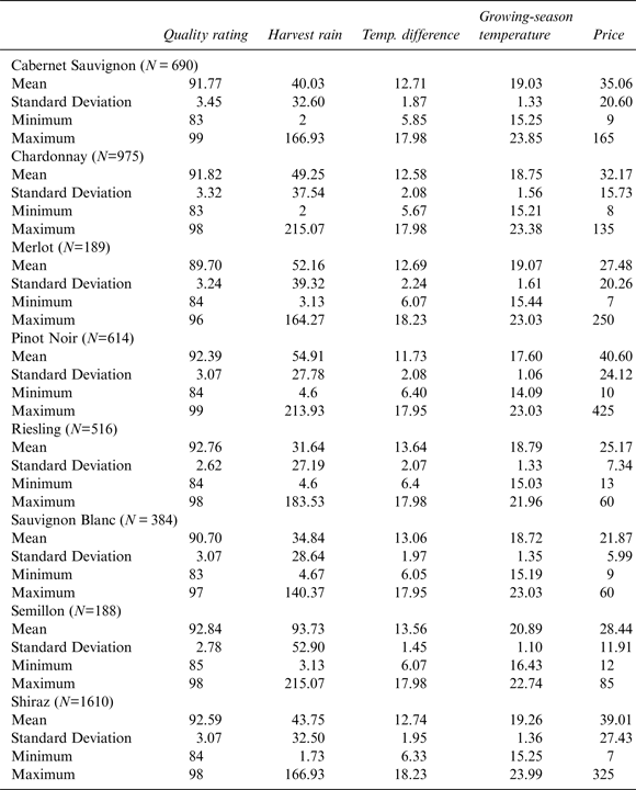
The summary statistics for the key variables and the eight varieties are provided in Table 1. Some of the main sample differences between varieties include higher average harvest rainfall for Semillon, which is predominantly grown in the Hunter Valley; lower average growing season temperature for Pinot Noir; and lower average prices for Sauvignon Blanc.
Summary Statistics

IV. Results
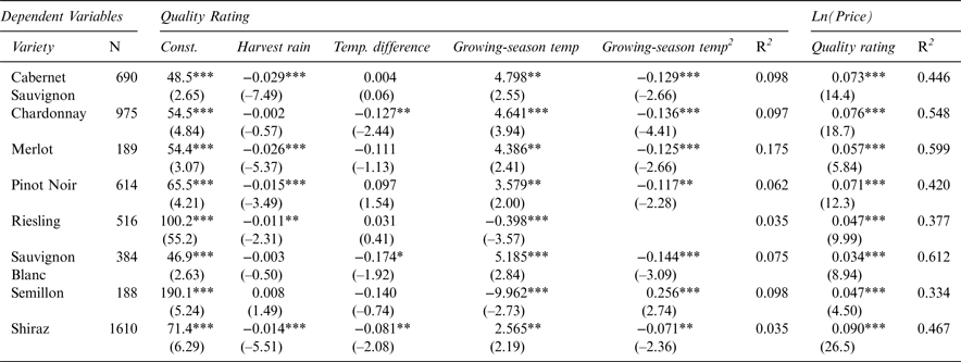
Parameter estimates for equation (1) and the marginal wine-quality impact on prices (β 1) for equation (2) are presented in Table 2. For equation (1) and quality ratings, the quadratic form for growing-season temperature was statistically significant for all varieties except Riesling, for which the linear form was appropriate. The explanatory power of the models ranges from 4% to 18% and averages about 8%, which tends to be at the lower range of results in other studies. This general result might confirm the relatively lower importance of weather in explaining quality variations in Australia compared to European countries. Harvest rain and the temperature differential have a statistically significant negative impact for five and three varieties, respectively. The negative impact of harvest rain appears to be most important for Cabernet Sauvignon and Merlot, while extreme temperature variations appear to affect Chardonnay and Sauvignon Blanc most.
Wine Quality Rating and Price Estimates
Notes: Robust t-ratios are in parentheses. ***, ** and * denote statistical significance at the 1%, 5%, and 10% respectively.
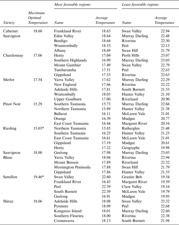
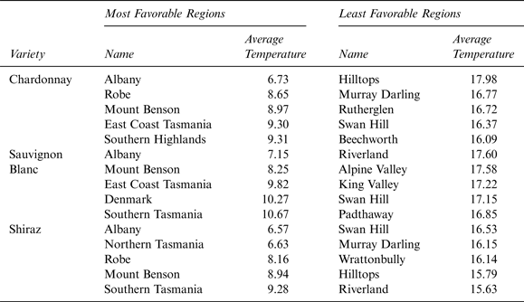
To examine the impact of growing-season temperature on wine quality, Table 3 presents the most and least favorable regions in relation to optimal growing temperatures for each variety. For six of the seven quadratic models (leaving out Semillon) the optimal temperature varies from 15.3° for Pinot Noir to 18.6° for Cabernet Sauvignon and averages 17.4°. These optimal temperatures are lower than sample average temperatures (see Table 1). Cabernet Sauvignon (–0.43) and Sauvignon Blanc (–0.72) have the closest to optimal average temperatures, while Pinot Noir (–2.31) has the largest difference between optimal and average temperatures. Interestingly, the optimal temperature for Shiraz (18.1°) is only slightly lower than that identified for the iconic Hill of Grace (18.6°) and Grange (19°). As expected, Pinot Noir and Chardonnay, being relatively early-ripening varieties, have lower optimal temperatures, while Cabernet Sauvignon and Shiraz, being midseason or relatively later-ripening varieties, have higher optimal temperatures. This variation points to the importance of modeling varieties separately in the analysis of temperature effects on wine quality.
Wine Quality and Growing-Season Temperature
* The lowest sample temperature is listed for Riesling given the negative linear specification. The minimum optimal temperature is listed for Semillon. Season average temperature (degrees Celsius) covers the months October to March, averaging the maximum and minimum average monthly temperatures.
In general, there appears to be significant variation between the varieties for the best growing-temperature regions, but most regions are in a relatively cool climate in the Australian context. There is much more consistency for the warmer least favorable regions for the various varieties, with Murray Darling and Riverina being prominent. Except for Pinot Noir and Riesling, the most favorable regions have average temperatures that are no more than 0.5° different from optimal temperatures. For Semillon, a minimum optimal temperature is listed given its estimates (Table 2), which implies that at low temperatures increasing temperature reduces quality, while at high temperatures increasing temperature increases quality. As a consequence, the best regions for quality Semillon production occur in both low and high seasonal-temperature regions, for example, Frankland River with 16.4° and Swan Valley with 22.6°. These differences reflect different styles of wine, which both result in high-quality scores. The negative linear relation for Riesling implies the lowest sample temperatures are optimal, and this is typical of Tasmanian regions.
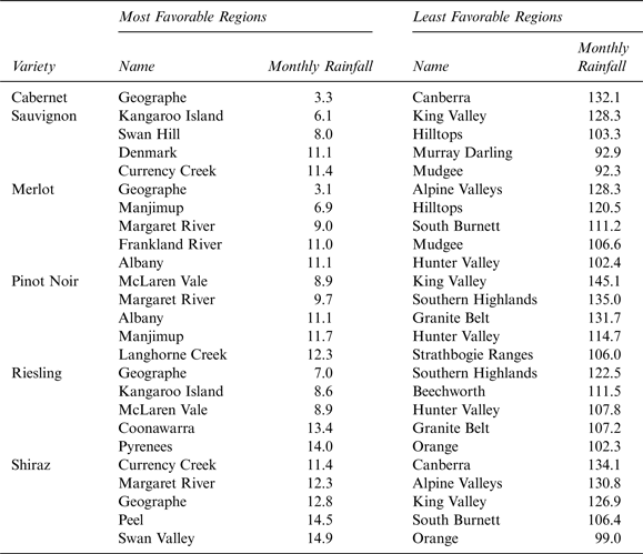
The most and least favorable regions for harvest rain and temperature differences are presented in Tables 4 and 5. These tables list the largest regional impacts of harvest rain and temperature differences on wine quality. Only varieties that have statistically significant effects (Table 2) are listed. For harvest rain, there is some relative consistency of regions across varieties. The southern part of Western Australia (Geographe, Manjimup, Margaret River) received relatively little harvest rain for the examined vintages, and hence wine quality suffered least due to excessive rain. The Hunter and King Valleys appear to be the areas affected most adversely from harvest rain for the vintages analyzed. There is significant consistency across varieties for the regions that suffer least because of excessive temperature variations, including Albany, Robe, Mount Benson, and parts of Tasmania. Wine quality in Swan Hill, Hilltops, Riverland, and the Murray Darling appears to be affected most adversely by temperature variations across the varieties analyzed.
Wine Quality and Harvest Rain
Average monthly rainfall (ml) for the months January to March.
Wine Quality and Temperature Difference
Temperature difference (degrees Celsius) covers the months October to March, averaging the difference between maximum and minimum average monthly temperatures.
As indicated in Table 2, all the quality-rating estimates on wine prices are highly significant, with prices estimated to increase by an average of 6.2% per rating point across all varieties. The smallest quality impact for price is 3.4% for Sauvignon Blanc, and the largest is 9.0% for Shiraz. The R 2s for equation (2) range from 0.33 to 0.60, which is broadly consistent with hedonic price models generally. The region and vintage variables are also relatively important for explaining price variations. Across all varieties, approximately 50% of regions are estimated to have a significant impact (10% level) compared to average sample prices. While vintage was statistically significant for all varieties except Merlot, vintage effects (measured using the vintage year) range from –4.3% for Pinot Noir to –13.2% for Shiraz per year, averaging –8.6% across all varieties.
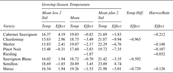
To examine the effects of weather on wine prices, we consider the indirect effect of weather on price using wine quality . This is estimated as the product of parameter estimates from equation (1) and β 1 from equation (2). These weather effects on prices are presented in Table 6. Given the quadratic relation for growing-season temperature for all varieties except Riesling, then its impact on price depends on the temperature level. As a consequence, seasonal temperature effects are presented at the mean and +/– two standard deviations . At sample mean seasonal temperature levels, all effects are negative (except on Semillon), which implies that a one-degree–Celsius-increase in temperature reduces prices by less than 1% for Cabernet Sauvignon and Sauvignon Blanc and by more than 3% for Chardonnay and Pinot Noir. At the low-end range of temperature levels (mean minus two standard deviations), increases in temperature increase prices for all varieties except for Pinot Noir and Semillon. For Pinot Noir, even lower temperature levels are needed for price rises. At the high-end range of temperature levels (mean plus two standard deviations) further increases in temperatures can have a large impact. Price falls of more than 5% for a one-degree increase in temperature are estimated for five of the varieties, and up to a 10% price fall for Chardonnay.
Weather Effects on Prices
Weather effects represents the percentage change impact on price from a unit change in the variable. Std represents the standard deviation.
For temperature differences, with sample standard deviations of about two, a one-standard-deviation increase in temperature difference reduces prices by 1.2% for Sauvignon Blanc and up to 2% for Chardonnay. The sample standard deviation for harvest rain is approximately 30 mls, and a one-standard-deviation increase in harvest rain reduces prices by from 1.4% for Riesling to 6.9% for Cabernet Sauvignon.
Finally, it is worth examining the veracity of the indirect modeling approach of weather effects on prices represented by equations (1) and (2), against alternatives. The average R 2 for explaining wine prices for equation (2) is 0.475. Adding the weather variables to equation (2), as considered by Haeger and Storchmann (Reference Haeger and Storchmann2006) and Ramirez (Reference Ramirez2008), raises the average R 2 by less than 1% to 0.484, with only harvest rainfall statistically significant (and positive) for three varieties. This implies that weather effects on prices are adequately captured by the quality ratings variable.
An alternative representation in which quality ratings are excluded from equation (2) and weather variables are included (in the spirit of Ashenfelter [2008], Byron and Ashenfelter [1985], and others) results in an average R 2 of 0.316, which explains approximately 16% less of the price variation than equation (2). Further, only harvest rain is statistically significant (and positive) for some varieties in the weather effects, region, and vintage model. The mean-encompassing non-nested test (Mizon and Richard, Reference Mizon and Richard1986), which develops a comprehensive model (both quality and weather) and tests for the alternative models using subset F tests, confirms the superiority of equation (2). For the comprehensive model, two F tests are conducted: a joint F test for the significance of all the weather variables from equation (1); and an F test for the significance of the quality-rating variable. Equation (2) strongly rejects the price model that directly includes weather for all varieties, with F statistics ranging from 24.7 to 714.7 and averaging 208.9. In contrast, equation (2) is rejected (at the 5% level) only by the direct weather model for Shiraz, with F statistics ranging from 0.55 to 3.40 and averaging 1.70. These results support the adopted indirect weather effects modeling approach for our data set.
V. Conclusion
This paper highlights a number of issues that may have wider applicability for the analysis of the impact of weather on wine prices. Serious consideration needs to be given to the assumed information set about weather conditions held by wine buyers. For very expensive iconic wines, for which auction prices dominate, given the expected significant financial outlay buyers are likely to have devoted, significant resources in ascertaining vintage weather information and weather conditions as such are likely to affect prices directly. In contrast, for a broad spectrum of different quality and generally available retail wines, it appears unlikely that consumers have specific knowledge of weather conditions, and as such these are less likely to affect prices directly. For our cross-section Australian data set, we demonstrate how wine-guide quality ratings explain retail prices significantly better than they do weather conditions. Effectively, among other things, quality ratings capture the impact of weather on prices.
The analysis of the impact of weather on prices needs to be monitored on a regular basis, given evidence that for some wines the impact of weather on prices may strengthen over the very long term (Chevet et al., Reference Chevet, Lecocq and Visser2011). In addition to year-on-year vintage changes, weather differences between regions are important for explaining wine-quality variations. The results in Tables 3 to 5 clearly point to the differential weather impact of Australian growing regions. Further, the results highlight the importance of analyzing wine varieties separately. Clear important differences with regard to growing-season temperatures emerge between varieties, with optimal temperatures varying as much as 3°. We show (Table 6) that changes in temperatures have differential impacts on prices, highly dependent on grape variety.
Finally, we note that for most varieties, the estimated optimal temperature was lower than sample average temperatures. This implies that, on average, most production occurs at seasonal temperatures that are higher than optimal. Over time, as average temperatures increase as a consequence of climate change, further differences between optimal and average temperatures may occur. This may necessitate the relocation of certain grape varieties to more suitable growing regions if wine prices are to be maintained. This and related weather issues will continue to demand significant attention as the impact of climate change on wine gains increasing prominence worldwide.