1 Introduction
Fluid flows of practical interest typically exhibit complex spatio-temporal behaviour, and the analysis of such flows frequently relies upon interrogating large collections of high-dimensional velocity field snapshots. A widely employed strategy is to attempt to extract coherent structures from the snapshots, that is, spatial features of dynamic importance to the flow that can be used to facilitate its analysis, modelling or control. For canonical flows, coherent structures such as vortex-shedding modes of bluff bodies flows (Choi and Kim Reference Choi, Jeon and Kim2008) or spatial streaks in wall-bounded flows (Orlandi Reference Orlandi1994) are well known, and the suppression of such structures may motivate a flow control strategy. However, for less-studied flows, coherent structures may not be known a priori and must therefore be sought directly from the snapshot data, necessitating the development of automatic, data-driven, structure extraction algorithms.
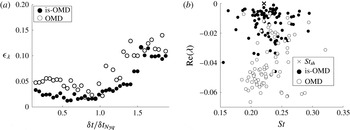
Perhaps the most widely used structure extraction methodology is proper orthogonal decomposition (POD) (Holmes, Lumley & Berkooz Reference Holmes, Lumley and Berkooz1996), which decomposes an ensemble of snapshots into orthogonal flow fields ranked by their energetic content. However, POD does not make use of the fact that underlying data are sampled from a dynamical system, meaning that low-energy, low-ranked structures may still be of importance to the system’s behaviour (Noack et al. Reference Noack, Afanasiev, Morzynski, Tadmor and Thiele2003). If the data are sampled at a constant time step, however, the dynamic mode decomposition (DMD) (Schmid Reference Schmid2010) can be applied to incorporate temporal information when extracting modes. DMD can be viewed either as fitting a low-order linear model to the evolution of temporal POD coefficients (Wynn et al. Reference Wynn, Pearson, Ganapathisubramani and Goulart2013) or, alternatively, as an approximation to the underlying Koopman operator of the system (Rowley et al. Reference Rowley, Mezic, Bagheri, Schlatter and Henningson2009). DMD has received much recent interest both in terms of its application to analysis of different classes of flows (such as bluff body flows (Muld, Efraimsson & Henningson Reference Muld, Efraimsson and Henningson2012; Bagheri Reference Bagheri2013; Tissot et al. Reference Tissot, Cordier, Benard and Noack2014), boundary layers (Grilli et al. Reference Grilli, Schmid, Hickel and Adams2012; Sayadi et al. Reference Sayadi, Schmid, Nichols and Moin2014), cavity flows (Schmid Reference Schmid2010; Seena & Sung Reference Seena and Sung2011; Vinha et al. Reference Vinha, Meseguer-Garrido, De Vicente and Valero2016) or jet flows (Rowley et al. Reference Rowley, Mezic, Bagheri, Schlatter and Henningson2009; Schmid Reference Schmid2010; Schmid, Violato & Scarano Reference Schmid, Violato and Scarano2012; Semeraro, Bellani & Lundell Reference Semeraro, Bellani and Lundell2012)) but also in terms of its theoretical development. In particular, a number of generalisations of the DMD algorithm have recently been proposed, with each seeking to address various deficiencies of the algorithm. Examples of the recent developments include: establishing an appropriate way of selecting the most important DMD modes (Chen, Tu & Rowley Reference Chen, Tu and Rowley2012; Jovanovic, Schmid & Nichols Reference Jovanovic, Schmid and Nichols2014), finding an optimal low-order projection basis (Wynn et al. Reference Wynn, Pearson, Ganapathisubramani and Goulart2013), improving the robustness of the method to observation noise (Wynn et al. Reference Wynn, Pearson, Ganapathisubramani and Goulart2013; Hemati, Rowley & Nichols Reference Hemati, Rowley and Nichols2017), establishing a stronger link to the Koopman operator (Williams, Kevrekidis & Rowley Reference Williams, Kevrekidis and Rowley2015) or accounting for input/output systems (Proctor, Brunton & Kutz Reference Proctor, Brunton and Kutz2014).
A fundamental requirement of dynamic mode extraction algorithms is that they must be applied to a data set of flow snapshots sampled at a constant time step
 $\unicode[STIX]{x1D6FF}t$
between subsequent snapshots. However, once
 $\unicode[STIX]{x1D6FF}t$
has been chosen, the Nyquist sampling criterion (Nyquist Reference Nyquist1928) indicates that an inherent limitation is placed upon the maximum frequency that can be extracted from a data set. This issue was discussed in Tu et al. (Reference Tu, Rowley, Kutz and Shang2014) in terms of current capabilities of PIV systems. The acquisition rate of a classical PIV system does not typically exceed 15 Hz, implying an upper limit upon the sampling rate which is not sufficient to investigate temporal characteristics of turbulent flows. Time-resolved PIV (TRPIV) systems exist that are capable of producing sampling rates in the range of 1–10 kHz (Adrian and Westerweel Reference Adrian and Westerweel2011), nonetheless, they still may not be sufficient to investigate frequencies of interest. Additionally, tomographic PIV (tomo-PIV) was introduced recently (Elsinga et al.
Reference Elsinga, Scarano, Wieneke and van Oudheusden2006), allowing the measurement of three velocity components. In such a case, the number of measurements drastically increases, especially in a combination with TRPIV systems, leading to high computational cost of the data processing and consequently establishing a need to obtain dynamical information from potentially undersampled data.
An attempt to extend the DMD algorithm to regularly undersampled data sets is presented in Leroux & Cordier (Reference Leroux and Cordier2016), where a low-dimensional state space is constructed using POD modes, missing snapshots are reconstructed using an Expectation–Maximisation algorithm and DMD modes are estimated as a solution to a multiple regression problem. However, perhaps the most widely employed methodology to extract coherence from temporally downsampled data is compressive sampling (Candes & Tao Reference Candes and Tao2006a ,Reference Candes, J. and Tao b ; Donoho Reference Donoho2006). Now, as will be discussed in § 2.2, compressive sampling is most effective at extracting sub-Nyquist frequency information in the situations where data snapshots are sampled randomly in time. This is at odds with the requirement of DMD-based modal extraction methodologies of a constant separation time step. In Tu et al. (Reference Tu, Rowley, Kutz and Shang2014) this problem was addressed by first performing compressive sampling directly on a temporally downsampled velocity field data ensemble, then subsequently using DMD to extract coherent structures. However, applying the compressive sampling algorithm requires one to pre-specify a basis such that representation of the data in the chosen basis is approximately sparse (see § 2.2). Such knowledge is often not available a priori. In this paper we propose an alternative to this strategy, the irregularly sampled optimal mode decomposition (is-OMD) algorithm. The motivation for our approach is to extend traditional modal extraction methods so that they can be applied to data sampled at non-constant time steps. Thus, the arbitrary choice of projection basis implied by a direct use of compressive sampling can be avoided, meaning that is-OMD provides a more flexible method for the analysis of high-dimensional temporally subsampled data ensembles. Further on, a proposed method makes use of already existing DMD-like algorithms, making is-OMD readily and easily implementable.
We discuss the performance of the is-OMD algorithm in terms of its ability to extract coherent spatial features with associated and accurate dynamical information, and whether such information can be used to reconstruct the instantaneous state of the flow from subsampled data. Section 2.1 provides an outline of the is-OMD algorithm followed by a rigorous stability analysis in § 3. A robust extension to the algorithm in terms of estimation of mode shapes and instantaneous unknown snapshots is presented in § 4. Section 5 demonstrates an example of a synthetic system for which is-OMD provides an improvement over compressive sampling in terms of frequency estimation, whilst § 6 provides a practical discussion of implementation of the algorithm to the canonical example of the cylinder wake. The demonstration of the applicability of the is-OMD algorithm to dynamically more complicated turbulent axisymmetric wake is presented in § 7.
2 Dynamic modes of downsampled and irregularly sampled data
Let
 $f(\boldsymbol{x},t)$
denote the state of a dynamical system which depends upon a spatial variable
 $\boldsymbol{x}$
and temporal variable
 $t$
. Suppose first that the system is sampled at
 $p$
spatial locations
 $(x_{i})_{i=1}^{p}$
and at equally spaced time steps
 $t_{n}=n\unicode[STIX]{x1D6FF}t$
to provide a data ensemble
 $$\begin{eqnarray}\boldsymbol{w}_{n}=(f(x_{i},t_{n}))_{i=1}^{p}\in \mathbb{R}^{p},\quad n=0,\ldots ,N.\end{eqnarray}$$
The DMD algorithm extracts dynamical information by approximating the evolution between subsequent snapshots. In particular, letting
 $\unicode[STIX]{x1D650}_{p}\in \mathbb{R}^{p\times N}$
be the matrix whose columns are the POD modes of the first
 $N$
snapshots
 $\{\boldsymbol{w}_{0},\ldots ,\boldsymbol{w}_{N-1}\}$
, DMD produces (Wynn et al.
Reference Wynn, Pearson, Ganapathisubramani and Goulart2013) a matrix
 $\unicode[STIX]{x1D64E}\in \mathbb{R}^{N\times N}$
which minimises the residual error
 $$\begin{eqnarray}\mathop{\sum }_{i=1}^{N}\Vert \boldsymbol{w}_{i+1}-\unicode[STIX]{x1D650}_{p}\unicode[STIX]{x1D64E}\unicode[STIX]{x1D650}_{p}^{\text{T}}w_{i}\Vert ^{2}.\end{eqnarray}$$
In other words, DMD searches for the optimal linear model to describe the evolution of a set of temporal POD coefficients over the time step
 $\unicode[STIX]{x1D6FF}t$
. Upon taking an eigenvalue decomposition
 $\unicode[STIX]{x1D64E}=\unicode[STIX]{x1D64B}\unicode[STIX]{x1D71F}\unicode[STIX]{x1D64B}^{-1}$
, the DMD modes of the system are defined to be the columns of
 $\unicode[STIX]{x1D650}_{p}\unicode[STIX]{x1D64B}$
, with each mode corresponding to an eigenvalue of
 $\unicode[STIX]{x1D64E}$
describing the mode’s growth rate and frequency.
Now, increasing the time step
 $\unicode[STIX]{x1D6FF}t$
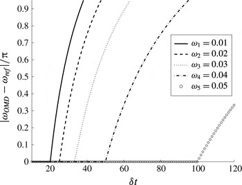
between sample points may decrease the accuracy of the extracted dynamical information. For a simple illustrative example, figure 1 shows the error between the true frequencies
 $(\unicode[STIX]{x1D714}_{j})_{j=1}^{5}=(j\unicode[STIX]{x03C0}10^{-2})_{j=1}^{5}$
and those identified by DMD from snapshots sampled from the one-dimensional sinusoidal system
 $$\begin{eqnarray}f(x,t)=\mathop{\sum }_{i=1}^{5}\sin (x+\unicode[STIX]{x1D714}_{i}t),\quad 0\leqslant x\leqslant 2\unicode[STIX]{x03C0},t\geqslant 0,\end{eqnarray}$$
for varying snapshot spacings
 $10\leqslant \unicode[STIX]{x1D6FF}t\leqslant 120$
. It can be seen that the error in each of the five system frequencies is zero until, respectively,
 $\unicode[STIX]{x1D6FF}t$
exceeds
 $100,50,33,25$
and
 $20$
. This corresponds exactly to the Nyquist condition that the sampling rate must be at least twice the frequency to be identified, that is,
 $\unicode[STIX]{x1D6FF}t\leqslant \unicode[STIX]{x03C0}/\unicode[STIX]{x1D714}_{j}=100/j$
. This presents the natural question of whether it is possible to reduce this error and correctly identify a system’s dynamical information in the case of undersampling. In signal processing, the established method for achieving such an aim is compressive sampling, which is typically applied to irregularly sampled data ensembles.
The error in frequency estimation for a range of uniform time steps between consecutive snapshots.

2.1 Irregularly sampled data
Consider the snapshots
 ${\mathcal{W}}=(\boldsymbol{w}_{n})_{n=0}^{N}\subset \mathbb{R}^{p}$
described in (2.1), sampled with constant time step
 $\unicode[STIX]{x1D6FF}t$
. An alternative to varying
 $\unicode[STIX]{x1D6FF}t$
, as discussed above, is to instead view
 $\unicode[STIX]{x1D6FF}t$
as a minimal time step representing the highest possible frequency of data collection, but assume that only a subset
 ${\mathcal{U}}\subset {\mathcal{W}}$
of snapshots may be used for analysis. We refer to
 ${\mathcal{U}}$
as the analysis data ensemble and define it by choosing a subset
 ${\mathcal{J}}\subset \{0,1,\ldots ,N\}$
, re-labelling
 $\boldsymbol{u}_{i}:=w_{i}$
for each index
 $i\in {\mathcal{J}}$
, and setting
 ${\mathcal{U}}=\{\boldsymbol{u}_{i}:i\in {\mathcal{J}}\}$
. Finally, let
 $\unicode[STIX]{x0394}t_{i}$
be the sample times between successive snapshots in
 ${\mathcal{U}}$
which are, possibly non-constant, integer multiples of
 $\unicode[STIX]{x1D6FF}t$
. The schematic representation of such a sampling strategy is presented in figure 2.
Downsampled and regularly sampled data.

It will be assumed that
 ${\mathcal{W}}$
is sampled at a sufficiently high rate that it contains all dynamical information of interest concerning the state trajectory
 $f(\boldsymbol{x},t)$
. The question which we aim to address is to what extent
 ${\mathcal{W}}$
can be reconstructed from knowledge of the analysis data set
 ${\mathcal{U}}$
only. Compressive sampling presents a standard method of answering such a problem.
2.2 Compressive sampling
Extracting coherent dynamical information from a downsampled data ensemble
 ${\mathcal{U}}$
may be possible if the underlying system is sparse, or compressible, when expressed in particular temporal basis. To describe this, first collect the high-frequency sampled snapshots
 ${\mathcal{W}}$
into a matrix
 $$\begin{eqnarray}\unicode[STIX]{x1D652}:=\left[\begin{array}{@{}ccc@{}}\uparrow & & \uparrow \\ \boldsymbol{w}_{0} & \cdots \, & \boldsymbol{w}_{N}\\ \downarrow & & \downarrow \end{array}\right]\in \mathbb{R}^{p\times (N+1)}.\end{eqnarray}$$
The state trajectory
 $\unicode[STIX]{x1D652}$
is said to be compressible if there exists a matrix
 $\unicode[STIX]{x1D729}=(\unicode[STIX]{x1D709}_{ij})\in \mathbb{R}^{(N+1)\times (N+1)}$
such that it can be approximately represented in the form
 $$\begin{eqnarray}\unicode[STIX]{x1D652}\approx \hat{\unicode[STIX]{x1D652}}\unicode[STIX]{x1D729},\end{eqnarray}$$
where
 $\hat{\unicode[STIX]{x1D652}}\in \mathbb{R}^{p\times N}$
is sparse in the sense that it has only
 $k$
non-zero columns, with
 $k\ll N$
. Letting
 $\hat{\boldsymbol{w}}_{i}$
denote the columns of
 $\hat{\boldsymbol{w}}$
, and rewriting the decomposition (2.5) as
 $$\begin{eqnarray}\boldsymbol{w}_{i}\approx \mathop{\sum }_{j=0}^{N}\hat{\boldsymbol{w}}_{j}\unicode[STIX]{x1D709}_{ji},\quad i=0,\ldots ,N,\end{eqnarray}$$
it is clear that the each column
 $\hat{\boldsymbol{w}}_{j}\in \mathbb{R}^{p}$
represents a spatial structure, while the respective row
 $(\unicode[STIX]{x1D709}_{ji})_{i=0}^{N}$
of
 $\unicode[STIX]{x1D729}$
describes its temporal evolution. For this discussion we make the assumption that a temporal basis
 $\unicode[STIX]{x1D729}$
is known for which a columnwise sparse solution
 $\hat{\unicode[STIX]{x1D652}}$
to (2.5) exists.
Next, write the analysis data ensemble
 ${\mathcal{U}}$
in matrix form
 $$\begin{eqnarray}\unicode[STIX]{x1D650}=\left[\begin{array}{@{}ccc@{}}\uparrow & & \uparrow \\ \boldsymbol{u}_{1} & \cdots \, & \boldsymbol{u}_{m}\\ \downarrow & & \downarrow \end{array}\right]=\unicode[STIX]{x1D652}\unicode[STIX]{x1D723},\end{eqnarray}$$
by defining an appropriate binary matrix
 $\unicode[STIX]{x1D723}\in \mathbb{R}^{N+1\times m}$
,
 $m=|{\mathcal{J}}|$
, which encodes the particular time steps at which data are available. The aim of compressive sampling is to determine
 $\unicode[STIX]{x1D652}$
from knowledge of
 $\unicode[STIX]{x1D650}$
only. In view of (2.5) and (2.7), one way to achieve this is to seek a columnwise sparse solution
 $\hat{\unicode[STIX]{x1D652}}$
to
 $$\begin{eqnarray}\unicode[STIX]{x1D650}=\hat{\unicode[STIX]{x1D652}}\unicode[STIX]{x1D729}\unicode[STIX]{x1D723},\end{eqnarray}$$
which would then provide an approximation to the full signal via
 $\unicode[STIX]{x1D652}\approx \hat{\unicode[STIX]{x1D652}}\unicode[STIX]{x1D729}$
.
Note that, since
 $m\leqslant N$
, equation (2.8) is overdetermined, meaning that the imposition of sparsity is necessary to obtain a well-posed problem. The most widely used approach to sparsity promotion is to penalise the
 $\ell ^{1}$
-norm of
 $\hat{\unicode[STIX]{x1D652}}$
subject to the constraint (2.8). However, apart from in the scalar-valued case
 $p=1$
, this will impose entrywise sparsity rather than the desired columnwise sparsity of
 $\hat{\unicode[STIX]{x1D652}}$
. Methods to avoid this problem typically use greedy algorithms such as orthogonal matching pursuit (OMP) (Tropp & Gilbert Reference Tropp and Gilbert2007) or compressive sampling matching pursuit (CoSaMP) (Needell & Tropp Reference Needell and Tropp2009). Rather than minimising the
 $\ell ^{1}$
-norm of
 $\hat{\unicode[STIX]{x1D652}}$
, such methodologies analyse the correlation of the matrix
 $\unicode[STIX]{x1D729}\unicode[STIX]{x1D723}$
with the downsampled data ensemble
 $\unicode[STIX]{x1D650}$
. They are iterative algorithms in which, upon each iteration, one sparse vector (a column of
 $\unicode[STIX]{x1D729}$
) is added to the solution. Hence, the outputs of the algorithms are sparse, with the sparsity of the solution equal to the number of iterations.
An important fact is that the sampling strategy, encoded by
 $\unicode[STIX]{x1D723}$
, plays a significant role in determining the performance of compressive sampling algorithms. In particular, a known requirement is that the chosen temporal basis
 $\unicode[STIX]{x1D729}$
has a low coherence with the sampling strategy
 $\unicode[STIX]{x1D723}$
(where coherence is defined
 $\max _{j,k}|\langle (\unicode[STIX]{x1D703}_{ji})_{i=0}^{N},(\unicode[STIX]{x1D709}_{ik})_{i=0}^{N}\rangle |$
) (Candes & Wakin Reference Candes and Wakin2008). A common way to achieve this is to use Bernoulli and Gaussian random measurements, which are known to be incoherent with many canonical bases, including the typical Fourier basis (Candes & Wakin Reference Candes and Wakin2008). That is, if periodic structures are sought in time, then an aperiodic sampling strategy is beneficial for extracting them from downsampled data. We reiterate that DMD-type modal extraction methods do not currently support sampling at non-constant time intervals, meaning that any potential benefits of such a strategy may not be realised using current techniques. We now expand upon this observation and propose an extension to DMD to enable its application to a general irregularly sampled data ensemble of the form
 ${\mathcal{U}}$
described in figure 2.
2.3 Dynamic decomposition of irregularly sampled data
The application of DMD to the regularly sampled data set
 ${\mathcal{W}}$
, as discussed above, can be obtained by minimising the cost (2.2) with respect to the dynamics matrix
 $\unicode[STIX]{x1D64E}$
. This cost function corresponds to projecting each snapshot
 $\boldsymbol{w}_{i}$
onto its POD coefficients via
 $\unicode[STIX]{x1D650}_{p}^{\text{T}}\boldsymbol{w}_{i}$
, transforming these coefficients under the mapping
 $\unicode[STIX]{x1D64E}$
, lifting the result back to create a modified flow field
 $\unicode[STIX]{x1D650}_{p}\unicode[STIX]{x1D64E}\unicode[STIX]{x1D650}_{p}^{\text{T}}\boldsymbol{w}_{i}$
, and finally comparing this flow field to the snapshot
 $\boldsymbol{w}_{i+1}$
. Consequently, DMD can be viewed in terms of constructing an optimal model of the form
 $\boldsymbol{w}_{i}\mapsto \unicode[STIX]{x1D650}_{p}\unicode[STIX]{x1D64E}\unicode[STIX]{x1D650}_{p}^{\text{T}}\boldsymbol{w}_{i}$
which best approximates the one-step snapshot evolution across the entire data ensemble. Solving the DMD optimisation problem is computationally undemanding: the calculation of
 $\unicode[STIX]{x1D650}_{p}$
is simply
 $\text{POD}(\boldsymbol{w}_{0},\ldots ,\boldsymbol{w}_{N-1})$
; while, since (2.2) is quadratic, an analytical solution for
 $\unicode[STIX]{x1D64E}$
can easily be obtained by differentiating the cost and solving the resulting linear equation (Wynn et al.
Reference Wynn, Pearson, Ganapathisubramani and Goulart2013).
Now, if one attempts to apply a similar approach to the irregularly sampled data ensemble
 ${\mathcal{U}}$
, a natural generalisation of (2.2) is to consider the modified cost function
 $$\begin{eqnarray}\mathop{\sum }_{i=0}^{N}\Vert \boldsymbol{u}_{i+1}-\unicode[STIX]{x1D650}_{p}\unicode[STIX]{x1D64E}^{n_{i}}\unicode[STIX]{x1D650}_{p}^{\text{T}}\boldsymbol{u}_{i}\Vert ^{2}=\mathop{\sum }_{i=0}^{N}\Vert \boldsymbol{w}_{i+n_{i}}-\unicode[STIX]{x1D650}_{p}\unicode[STIX]{x1D64E}^{n_{i}}\unicode[STIX]{x1D650}_{p}^{\text{T}}\boldsymbol{w}_{i}\Vert ^{2},\end{eqnarray}$$
where
 $n_{i}:=\unicode[STIX]{x0394}t_{i}/\unicode[STIX]{x1D6FF}t\in \mathbb{N}$
is the number of minimal time steps
 $\unicode[STIX]{x1D6FF}t$
between each sample point in
 ${\mathcal{U}}$
. In other words, if there are
 $n_{i}$
minimal time steps between available data vectors
 $\boldsymbol{u}_{i+1}$
and
 $\boldsymbol{u}_{i}$
we seek to model the system evolution over an interval of length
 $\unicode[STIX]{x0394}t_{i}=n_{i}\unicode[STIX]{x1D6FF}t$
by the iterated linear mapping
 $(\unicode[STIX]{x1D650}_{p}\unicode[STIX]{x1D64E}\unicode[STIX]{x1D650}_{p}^{\text{T}})^{n_{i}}=\unicode[STIX]{x1D650}_{p}\unicode[STIX]{x1D64E}^{n_{i}}\unicode[STIX]{x1D650}_{p}^{\text{T}}$
.
Such a formulation encounters two immediate problems. First, the DMD choice of
 $\unicode[STIX]{x1D650}_{p}=\text{POD}(\boldsymbol{w}_{0},\ldots ,\boldsymbol{w}_{N-1})$
cannot be made since
 ${\mathcal{U}}$
may not contain all such data snapshots. Second, and more importantly, since in general
 $n_{i}>1$
, the modified cost (2.9) is at least of quartic order with respect to
 $\unicode[STIX]{x1D64E}$
, meaning that an analytical solution is no longer available. To attempt to avoid these problems, consider the related optimisation problem
 $$\begin{eqnarray}\displaystyle & \displaystyle \underset{\hat{\unicode[STIX]{x1D74E}}_{i},\unicode[STIX]{x1D647},\unicode[STIX]{x1D648}}{\min }\mathop{\sum }_{i=0}^{N}\Vert \hat{\unicode[STIX]{x1D74E}}_{i+1}-\unicode[STIX]{x1D647}\unicode[STIX]{x1D648}\unicode[STIX]{x1D647}^{\text{T}}\hat{\unicode[STIX]{x1D74E}}_{i}\Vert ^{2}, & \displaystyle\end{eqnarray}$$
 $$\begin{eqnarray}\displaystyle & \displaystyle \text{s.t. }\hat{\unicode[STIX]{x1D74E}}_{i}\in \mathbb{R}^{p},\quad i=0,\ldots ,N, & \displaystyle\end{eqnarray}$$
 $$\begin{eqnarray}\displaystyle & \displaystyle \hat{\unicode[STIX]{x1D74E}}_{i}=\boldsymbol{u}_{i},\quad i\in {\mathcal{J}}, & \displaystyle\end{eqnarray}$$
 $$\begin{eqnarray}\displaystyle & \displaystyle \unicode[STIX]{x1D647}^{\text{T}}\unicode[STIX]{x1D647}=\unicode[STIX]{x1D644},\quad \unicode[STIX]{x1D647}\in \mathbb{R}^{p\times r},\quad \unicode[STIX]{x1D648}\in \mathbb{R}^{r\times r}. & \displaystyle\end{eqnarray}$$
Now, the variable space of (2.10) is considerably extended with respect to DMD. The low-order model
 $\hat{\unicode[STIX]{x1D74E}}_{i}\mapsto \unicode[STIX]{x1D647}\unicode[STIX]{x1D648}\unicode[STIX]{x1D647}^{\text{T}}\hat{\unicode[STIX]{x1D74E}}_{i}$
approximating snapshot evolution over one minimal time step
 $\unicode[STIX]{x1D6FF}t$
now has both its projective component
 $\unicode[STIX]{x1D647}$
and dynamics matrix
 $\unicode[STIX]{x1D648}$
as optimisation variables. This is the approach taken in the OMD algorithm (Wynn et al.
Reference Wynn, Pearson, Ganapathisubramani and Goulart2013) and avoids the need to calculate POD modes. More importantly, higher powers of the dynamics matrix
 $\unicode[STIX]{x1D648}$
are avoided by introducing ‘slack’ state variables
 $\hat{\unicode[STIX]{x1D74E}}_{\boldsymbol{j}}\in \mathbb{R}^{p}$
corresponding to each underlying minimal time step
 $j\unicode[STIX]{x1D6FF}t$
. The analysis data ensemble
 ${\mathcal{U}}$
is then employed by enforcing the constraint
 $\hat{\unicode[STIX]{x1D74E}}_{i}=\boldsymbol{u}_{i},i\in {\mathcal{J}}$
. Finally, again following the OMD formulation, the user-defined parameter
 $r\leqslant N-1$
specifies the rank of the sought approximating dynamics
 $\unicode[STIX]{x1D647}\unicode[STIX]{x1D648}\unicode[STIX]{x1D647}^{\text{T}}$
. For completeness, we note that (2.10) reduces to the DMD algorithm in the case that
 ${\mathcal{W}}={\mathcal{U}},r=N-1$
and
 $\unicode[STIX]{x1D647}=\text{POD}(\boldsymbol{w}_{0},\ldots ,\boldsymbol{w}_{N-1})$
. The OMD algorithm is recovered in the case that
 ${\mathcal{W}}={\mathcal{U}}$
.
Schematic representation of a single iteration of the is-OMD algorithm. Given an initial guess for the dynamics
 $\unicode[STIX]{x1D647}\unicode[STIX]{x1D648}\unicode[STIX]{x1D647}^{\text{T}}$
– represented by solid lines – over each time step and the slack variables (step 1), the slack variables are first updated (step 2) before being fixed to allow an update of
 $\unicode[STIX]{x1D647}$
and
 $\unicode[STIX]{x1D648}$
(step 3).

Despite the removal of higher orders of
 $\unicode[STIX]{x1D648}$
from the cost function, (2.10) cannot be solved directly. Indeed, the inclusion of the slack state variables
 $\hat{\unicode[STIX]{x1D74E}}_{i}\in \mathbb{R}^{p}$
makes the problem overdetermined, while the products of decision variables – for example, in the
 $\unicode[STIX]{x1D647}\unicode[STIX]{x1D648}\unicode[STIX]{x1D647}^{\text{T}}\hat{\unicode[STIX]{x1D74E}}_{i}$
term – indicate that the problem is non-convex. To begin to address these difficulties, we propose a two-step iterative solution method indicated schematically in figure 3: first, the model variables
 $\unicode[STIX]{x1D647}$
and
 $\unicode[STIX]{x1D648}$
are fixed and the slack variables
 $\hat{\unicode[STIX]{x1D74E}}_{i}$
are updated by solving a least-squares problem; second, the updated slack state variables are fixed, allowing
 $\unicode[STIX]{x1D648}$
and
 $\unicode[STIX]{x1D647}$
to be updated using the standard OMD algorithm applied to the regularly temporally sampled fields
 $\hat{\unicode[STIX]{x1D74E}}_{i}$
.
The first of these steps – minimising (2.10a
) with respect to
 $\hat{\unicode[STIX]{x1D74E}}_{i}$
only, subject to constraints (2.10b
), (2.10c
) – is simply a least-squares problem. However, since typically
 $p=\mathit{O}(10^{5-6})$
, the problem is memory-intensive and likely to be ill-conditioned. Instead, we only seek to minimise the model error over the subspace
 $\text{Im}(\unicode[STIX]{x1D647})\subset \mathbb{R}^{p}$
, where
 $\unicode[STIX]{x1D647}$
is fixed within the slack variable update subiteration. This is achieved by considering the projected quadratic cost
 $$\begin{eqnarray}\Vert \unicode[STIX]{x1D647}\unicode[STIX]{x1D647}^{\text{T}}\left(\hat{\unicode[STIX]{x1D74E}}_{i+1}-\unicode[STIX]{x1D647}\unicode[STIX]{x1D648}\unicode[STIX]{x1D647}^{\text{T}}\hat{\unicode[STIX]{x1D74E}}_{i}\right)\Vert ^{2}=\Vert \unicode[STIX]{x1D647}\left(\unicode[STIX]{x1D647}^{\text{T}}\hat{\unicode[STIX]{x1D74E}}_{i}-\unicode[STIX]{x1D648}\unicode[STIX]{x1D647}^{\text{T}}\hat{\unicode[STIX]{x1D74E}}_{i}\right)\Vert ^{2}=\Vert \boldsymbol{c}_{i+1}-\unicode[STIX]{x1D648}\boldsymbol{c}_{i}\Vert ^{2},\end{eqnarray}$$
where
 $\boldsymbol{c}_{i}:=\unicode[STIX]{x1D647}^{\text{T}}\hat{\unicode[STIX]{x1D74E}}_{i}\in \mathbb{R}^{r}$
. Since
 $r\ll p$
, minimising (2.11) with respect to
 $\boldsymbol{c}_{i}$
is advantageous to minimising (2.10a
) with respect to
 $\hat{\unicode[STIX]{x1D74E}}_{i}$
. Consequently, the first step of the pairwise optimisation is to solve the constrained least-squares problem
 $$\begin{eqnarray}\displaystyle & \displaystyle \underset{\boldsymbol{c}_{i}}{\min }\mathop{\sum }_{i=0}^{N}\Vert \boldsymbol{c}_{i+1}-\unicode[STIX]{x1D648}\boldsymbol{c}_{i}\Vert ^{2}, & \displaystyle\end{eqnarray}$$
 $$\begin{eqnarray}\displaystyle & \displaystyle \text{s.t. }\boldsymbol{c}_{i}=\unicode[STIX]{x1D647}^{\text{T}}\boldsymbol{u}_{i},\text{if}\;i\in {\mathcal{J}}, & \displaystyle\end{eqnarray}$$
 $$\begin{eqnarray}\displaystyle & \displaystyle \boldsymbol{c}_{i}\in \mathbb{R}^{r}, & \displaystyle\end{eqnarray}$$
 $\hat{\unicode[STIX]{x1D74E}}_{i}\leftarrow \unicode[STIX]{x1D647}\boldsymbol{c}_{i}$
. After this update, the
 $\hat{\unicode[STIX]{x1D74E}}_{i}$
are fixed and
 $\unicode[STIX]{x1D647},\unicode[STIX]{x1D648}$
are updated via the OMD algorithm
 $[\unicode[STIX]{x1D647},\unicode[STIX]{x1D648}]\leftarrow \text{OMD}((\hat{\unicode[STIX]{x1D74E}}_{i})_{i=0}^{N})$
. It is proved in appendix A that this two-step procedure is guaranteed to decrease the cost (2.10a
) which, being bounded below, implies that it will converge asymptotically.
A subtle characteristic of the OMD algorithm (step 6 in algorithm 1) is that the cost function of the minimisation problem (2.13) is invariant under rotations of
 $\unicode[STIX]{x1D647}$
(Wynn et al.
Reference Wynn, Pearson, Ganapathisubramani and Goulart2013). In particular, for any orthogonal matrix
 $\tilde{\unicode[STIX]{x1D64D}}$
such that
 $\tilde{\unicode[STIX]{x1D64D}}^{\text{T}}\tilde{\unicode[STIX]{x1D64D}}=\unicode[STIX]{x1D644}$
, the pairs
 $[\unicode[STIX]{x1D647},\unicode[STIX]{x1D648}]$
and
 $[\unicode[STIX]{x1D647}\tilde{\unicode[STIX]{x1D64D}},\tilde{\unicode[STIX]{x1D64D}}^{\text{T}}\unicode[STIX]{x1D648}\tilde{\unicode[STIX]{x1D64D}}]$
have equivalent costs. The explanation of this behaviour is that OMD identifies a subspace
 $\text{Im}(\unicode[STIX]{x1D647})\subset \mathbb{R}^{p}$
upon which a low-order representation of the system dynamics can be provided, and that each
 $\unicode[STIX]{x1D647}\tilde{\unicode[STIX]{x1D64D}}$
is just a member of the same equivalence class describing this subspace. For visualisation purposes, we therefore propose in steps 10–12 of algorithm 1 to choose a rotation of
 $\unicode[STIX]{x1D647}$
which ranks its columns by their energetic contribution to the known data.
The is-OMD procedure is summarised in algorithm 1 which outputs: (i) estimated intermediate snapshots
 $\boldsymbol{w}_{i},i\notin {\mathcal{J}}$
; (ii) a projection matrix
 $\unicode[STIX]{x1D647}$
and (iii) an approximate dynamics matrix
 $\unicode[STIX]{x1D648}$
. The appropriate choice of initial projection and dynamics matrices,
 $\unicode[STIX]{x1D647}_{0}$
,
 $\unicode[STIX]{x1D648}_{0}$
, will be discussed in detail in § 6.1 where it is demonstrated that a sensible choice is to set the initial dynamics matrix to be a small perturbation of the identity matrix with normal distribution of standard deviation
 $\unicode[STIX]{x1D70E}$
,
 $(\unicode[STIX]{x1D648}_{0})_{ij}=N(0,\unicode[STIX]{x1D70E}^{2})+\unicode[STIX]{x1D6FF}_{ij}$
, and the projection space to be POD modes of the analysis data ensemble
 ${\mathcal{U}}$
,
 $\unicode[STIX]{x1D647}_{0}=\text{POD}({\mathcal{U}})$
. Additionally, the beneficial impact of choosing a large value of
 $r$
will be established in § 6.2.

A natural variant of algorithm 1 is to use DMD in place of OMD in step 6, in which case
 $\unicode[STIX]{x1D647}_{k}:=\text{POD}((\boldsymbol{w}_{i}^{k})_{i=0}^{N})$
would be fixed in step 6 within each iteration. Note that in this case, a final rotation of
 $\unicode[STIX]{x1D647}$
in steps 10–12 is unnecessary. Finally, it should be noted that the notion of dynamic modes has not yet been defined in the context of algorithm 1. This will be discussed subsequently in § 4.1.
3 Algorithmic considerations
We now discuss feasibility of the slack variable subproblem (2.13) and computational complexity of the algorithm 1. Since the model update subproblem (2.14) is an application of OMD or DMD, we refer to (Wynn et al.
Reference Wynn, Pearson, Ganapathisubramani and Goulart2013) for a discussion of this step’s performance. Furthermore a detailed proof demonstrating that the cost
 $(S_{k})$
is monotone decreasing (and hence, convergent) is presented in appendix A.
3.1 Convexity of the slack variable update
The equality constrains
 $\boldsymbol{c}_{i}=\unicode[STIX]{x1D647}^{\text{T}}\boldsymbol{u}_{i},i\in {\mathcal{J}}$
of (2.13) represent time steps at which data are available. Without loss of generality, we consider the problem in which
 ${\mathcal{J}}=\{0,N\}$
, since the general optimisation problem can be broken into a number of independent subproblems of this form. Now, it is not difficult to prove that (2.13) can be written as the unconstrained least-squares problem
 $$\begin{eqnarray}\underset{\unicode[STIX]{x1D743}}{\min }\Vert \unicode[STIX]{x1D63C}\unicode[STIX]{x1D743}-\boldsymbol{b}\Vert _{2}^{2},\end{eqnarray}$$
where
 $$\begin{eqnarray}\unicode[STIX]{x1D63C}=\left[\begin{array}{@{}cccc@{}}\unicode[STIX]{x1D648} & 0 & \ldots \, & 0\\ -\unicode[STIX]{x1D644} & \ddots & \ddots & \vdots \\ 0 & \ddots & \ddots & 0\\ \vdots & \ddots & \ddots & \unicode[STIX]{x1D648}\\ 0 & \ldots \, & 0 & -\unicode[STIX]{x1D644}\\ \end{array}\right]\in \mathbb{R}^{Nr\times (N-1)r},\quad \boldsymbol{b}=\left[\begin{array}{@{}c@{}}\unicode[STIX]{x1D647}^{\text{T}}\boldsymbol{u}_{N}\\ 0\\ \vdots \\ 0\\ -\unicode[STIX]{x1D648}\unicode[STIX]{x1D647}^{\text{T}}\boldsymbol{u}_{1}\\ \end{array}\right]\in \mathbb{R}^{Nr},\end{eqnarray}$$
and
 $\unicode[STIX]{x1D743}=\left(\begin{array}{@{}c@{}}\boldsymbol{c}_{N-1}^{\text{T}}\cdots \boldsymbol{c}_{1}^{\text{T}}\end{array}\right)^{\text{T}}\in \mathbb{R}^{(N-1)r}$
. Consequently, (2.13) is convex and admits the solution
 $\unicode[STIX]{x1D743}=(\unicode[STIX]{x1D63C}^{\text{T}}\unicode[STIX]{x1D63C})^{-1}\unicode[STIX]{x1D63C}^{\text{T}}\boldsymbol{b}$
provided the matrix
 $\unicode[STIX]{x1D63C}$
is full rank. This is true, and follows from the easily shown fact that
 $\unicode[STIX]{x1D63C}\unicode[STIX]{x1D743}=0\Leftrightarrow \unicode[STIX]{x1D743}=0$
. Finally, we note that solving a series of independent subproblems has significant advantages in terms of computational memory savings and improved numerical stability due to a reduced condition number of
 $(\unicode[STIX]{x1D63C}^{\text{T}}\unicode[STIX]{x1D63C})$
compared to the case where
 $\unicode[STIX]{x1D743}$
and
 $\boldsymbol{b}$
contain
 $\unicode[STIX]{x1D647}^{\text{T}}\boldsymbol{u}_{i}$
and
 $\boldsymbol{c}_{i}$
for all
 $i\in {\mathcal{J}}$
.
3.2 Computational complexity
The computational cost of the algorithm 1 consists of that associated with the two optimisation subproblems; the least-squares problem (2.13) and the modal optimisation (2.14) where dynamic model is updated via OMD (or DMD). Solving the least-squares problem using, for example, the Moore–Penrose pseudoinverse of
 $\unicode[STIX]{x1D63C}\in \mathbb{R}^{Nr\times (N-1)r}$
has complexity
 $\mathit{O}(N^{3}r^{3})$
. Moreover, as discussed in § 3.1 the full least-squares problem can be broken down into a number of smaller, independent, subproblems corresponding to
 $N_{i}$
intermediate time steps, each of which can be solved at a low computation burden. For example,
 $(N_{i}=10,r=40)$
and
 $(N_{i}=20,r=60)$
can be solved in
 $0.01~\text{s}$
and
 $0.3~\text{s}$
on a standard desktop computer, respectively, and each subproblem could be parallelised, if required.
For the modal optimisation subproblem (2.14), a discussion of the computational performance of OMD and DMD can be found in (Wynn et al.
Reference Wynn, Pearson, Ganapathisubramani and Goulart2013). Both the total number of slack variables
 $N$
and the approximation rank
 $r$
affect computation time in addition to the underlying dynamic characteristics of the specific system to which the each algorithm is applied. With respect to the examples considered subsequently: for the cylinder flow in § 6, the is-OMD algorithm converges with a tolerance of
 $10^{-2}$
after
 $80$
iterations of algorithm 1, with each call of OMD in subproblem (2.14) requiring
 $8.0~\text{s}~(N=500,r=50)$
, giving a total computation time for is-OMD of
 $640~\text{s}$
; for the application to PIV snapshots of turbulent flow past an axisymmetric bluff body in § 7, is-OMD converges to the same tolerance in only
 $10$
iterations but with a higher cost of
 $13.8~\text{s}~(N=120,r=30)$
for each OMD subproblem, resulting in a total computation time of
 $138~\text{s}$
.
Finally, we note that since both OMD and algorithm 1 are iterative, a possible method to improve algorithmic efficiency would be to apply a (small) fixed number of OMD iterates at each subproblem (2.14). Alternatively, one may apply DMD in place of OMD in subproblem (2.14) to reduce the computational cost. This will be explored in future work. All computations were performed using MATLAB on a standard desktop PC with a 3.4 GHz quad-core Intel i7 processor and 16 GB RAM.
4 Mode extraction and approximation of intermediate snapshots
In order to describe the performance of algorithm 1, consider first a one-dimensional synthetic sinusoidal system
 $$\begin{eqnarray}f(\boldsymbol{x},t)=\mathop{\sum }_{j}A_{j}\sin (k_{i}\boldsymbol{x}+\unicode[STIX]{x1D714}_{j}t)\exp (\unicode[STIX]{x1D6FE}_{j}t),\quad 0\leqslant \boldsymbol{x}\leqslant 1,t>0,\end{eqnarray}$$
with exponential growth rates
 $\unicode[STIX]{x1D6FE}_{j}$
, amplitudes
 $A_{j}>0$
, frequencies
 $\unicode[STIX]{x1D714}_{j}>0$
and wavenumbers
 $k_{j}>0$
. A reference data set
 ${\mathcal{W}}=\{\boldsymbol{w}_{i}\}_{i=1}^{900}$
is created where each snapshot
 $$\begin{eqnarray}\boldsymbol{w}_{i}=\left(f\left(\frac{j}{N_{x}},i\unicode[STIX]{x1D6FF}t\right)\right)_{j=0}^{N_{x}},\quad i=1,\ldots ,900,\end{eqnarray}$$
is sampled at
 $N_{x}=10^{4}$
equally spaced points.
Downsampled, analysis data sets
 ${\mathcal{U}}=\{\boldsymbol{w}_{i}\}_{i\in {\mathcal{J}}}\subset {\mathcal{W}}$
are created by defining a subsampling strategy
 ${\mathcal{J}}\subset \{1,\ldots ,N\}$
, and associated with each downsampled set is an average sampling time step
 $$\begin{eqnarray}\unicode[STIX]{x0394}t_{av}:=\frac{1}{|{\mathcal{J}}|}\mathop{\sum }_{i\in {\mathcal{J}}}\unicode[STIX]{x0394}t_{i},\end{eqnarray}$$
where
 $\unicode[STIX]{x0394}t_{i}$
is the time step between subsequent elements of
 ${\mathcal{U}}$
. For each frequency
 $\unicode[STIX]{x1D714}_{j}$
, let
 $\unicode[STIX]{x1D6FF}t_{j}^{\ast }:=\unicode[STIX]{x03C0}/\unicode[STIX]{x1D714}_{j}$
denote the largest sampling time step which satisfies the Nyquist criterion for that particular frequency. Of interest will be the situations in which
 $\unicode[STIX]{x0394}t_{av}/\unicode[STIX]{x1D6FF}t_{j}^{\ast }>1$
, indicating cases where, on average, downsampling may prevent accurate frequency identification.
We consider data sampled from (4.1) in the case of two frequencies
 $\unicode[STIX]{x1D714}_{1}=\unicode[STIX]{x03C0}/20,\unicode[STIX]{x1D714}_{2}=2\unicode[STIX]{x03C0}/25$
, respective amplitudes
 $A_{1}=1,A_{2}=0.5$
, wavenumbers
 $k_{1}=10,k_{2}=100$
, growth rates
 $\unicode[STIX]{x1D6FE}_{1}=0.01,\unicode[STIX]{x1D6FE}_{2}=0.05$
and minimal time step
 $\unicode[STIX]{x1D6FF}t=1$
. The analysis data ensemble
 ${\mathcal{U}}$
is selected with an average sampling time step satisfying
 $$\begin{eqnarray}\frac{\unicode[STIX]{x0394}t_{av}}{\unicode[STIX]{x1D6FF}t_{1}^{\ast }}=\frac{7}{8},\quad \frac{\unicode[STIX]{x0394}t_{av}}{\unicode[STIX]{x1D6FF}t_{2}^{\ast }}=\frac{6}{5},\end{eqnarray}$$
meaning that we would expect, according to the Nyquist criterion, to accurately extract
 $\unicode[STIX]{x1D714}_{1}$
but not
 $\unicode[STIX]{x1D714}_{2}$
. Such a selection of an average sampling time step provides a downsampled data ensemble
 ${\mathcal{U}}$
of cardinality
 $|{\mathcal{U}}|=45$
, i.e. only 5 % of the time-resolved ensemble
 ${\mathcal{W}}$
is retained. Algorithm 1 is initialised with
 $(\unicode[STIX]{x1D648}_{0})_{ij}=N(0,\unicode[STIX]{x1D70E}^{2})+\unicode[STIX]{x1D6FF}_{ij}$
, that is, a small perturbation of the identity matrix with
 $\unicode[STIX]{x1D70E}=\sqrt{0.3}$
, and
 $\unicode[STIX]{x1D647}_{0}=\text{POD}(\unicode[STIX]{x1D650})$
, where
 $\unicode[STIX]{x1D650}$
is the analysis data ensemble in a matrix form.
Figure 4 presents the eigenvalues of the matrix
 $\unicode[STIX]{x1D648}$
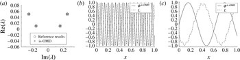
obtained from the is-OMD algorithm, demonstrating that the is-OMD algorithm accurately identifies the oscillatory and exponential parts of the dynamics corresponding to both resolved and undersampled frequencies. For results presented in figure 4 the proportional eigenvalue error is
 $\mathit{O}(10^{-6})$
for both
 $\unicode[STIX]{x1D706}_{1}$
and
 $\unicode[STIX]{x1D706}_{2}$
. Additionally, figure 4 presents the most energetic columns of
 $\unicode[STIX]{x1D647}$
. These structures have the shape of sinusoids with an amplitude and wavenumber specified by
 $A_{j}$
and
 $k_{j}$
. Columns of
 $\unicode[STIX]{x1D647}$
retain the prescribed values of
 $k_{j}$
, albeit with a visible interaction between
 $k_{1}$
and
 $k_{2}$
.
Dynamic matrix
 $\unicode[STIX]{x1D648}$
obtained using the is-OMD algorithm for the synthetic sinusoidal system with exponential dynamics (a), structures present in the system corresponding to
 $k=100$
(b) and to
 $k=10$
(c) represented by most energetic columns of
 $\unicode[STIX]{x1D647}$
and is-OMD modes
 $\unicode[STIX]{x1D731}^{is\text{-}OMD}$
obtained using algorithm 2.

As discussed in § 2.3, the columns of
 $\unicode[STIX]{x1D647}$
should be viewed as spanning a subspace of
 $\mathbb{R}^{p}$
appropriate to the system dynamics and, consequently, there is no direct correspondence between eigenvalues of
 $\unicode[STIX]{x1D648}$
and columns of
 $\unicode[STIX]{x1D647}$
. In the OMD algorithm, dynamic modes
 $\unicode[STIX]{x1D731}$
are defined as the embedding of the eigenvectors of
 $\unicode[STIX]{x1D648}$
into a high-dimensional vector space using projection
 $\unicode[STIX]{x1D647}$
, i.e.
 $\unicode[STIX]{x1D731}=\unicode[STIX]{x1D647}\unicode[STIX]{x1D64B}$
, where
 $\unicode[STIX]{x1D648}=\unicode[STIX]{x1D64B}\unicode[STIX]{x1D6EC}\unicode[STIX]{x1D64B}^{-1}$
, indicating that each mode corresponds directly to a particular eigenvalue. Now, despite the identification of accurate spectral information and projection basis vectors indicated in figure 4, it is the case that the columns of
 $\unicode[STIX]{x1D647}\unicode[STIX]{x1D64B}$
lack coherence. In particular, the lack of time-resolved data manifests itself in corrupting the eigenvectors of
 $\unicode[STIX]{x1D648}$
. Although
 $\unicode[STIX]{x1D647}$
and
 $\unicode[STIX]{x1D648}$
may still be of sufficient quality to construct an approximate low-order model of the system, if one would like to define dynamic modes the following alternative mode extraction post-processing step is proposed.
4.1 Dynamic mode extraction
Given a data ensemble
 $(\boldsymbol{w}_{i})_{i=0}^{N}$
, a typical description (Rowley et al.
Reference Rowley, Mezic, Bagheri, Schlatter and Henningson2009; Schmid Reference Schmid2010; Chen et al. Reference Chen, Tu and Rowley2012) of dynamic modes
 $\unicode[STIX]{x1D731}_{i}$
and eigenvalues
 $\unicode[STIX]{x1D706}_{i}$
is that they describe the evolution of the first
 $N-1$
snapshots according to
 $$\begin{eqnarray}\boldsymbol{w}_{i}=\mathop{\sum }_{j=1}^{N}\unicode[STIX]{x1D706}_{j}^{i}\unicode[STIX]{x1D731}_{j}\Rightarrow \unicode[STIX]{x1D652}=\unicode[STIX]{x1D731}\unicode[STIX]{x1D651},\end{eqnarray}$$
where
 $\unicode[STIX]{x1D652}=[\boldsymbol{w}_{0},\ldots ,\boldsymbol{w}_{N-1}],\unicode[STIX]{x1D731}=[\unicode[STIX]{x1D731}_{1},\ldots ,\unicode[STIX]{x1D731}_{N}]$
and
 $\unicode[STIX]{x1D651}$
is the Vandermonde matrix
 $$\begin{eqnarray}\unicode[STIX]{x1D651}:=\left[\begin{array}{@{}ccccc@{}}1 & \unicode[STIX]{x1D706}_{1} & \unicode[STIX]{x1D706}_{1}^{2} & \cdots \, & \unicode[STIX]{x1D706}_{1}^{N-1}\\ 1 & \unicode[STIX]{x1D706}_{2} & \unicode[STIX]{x1D706}_{2}^{2} & \cdots \, & \unicode[STIX]{x1D706}_{2}^{N-1}\\ \vdots & \vdots & \vdots & \ddots & \vdots \\ 1 & \unicode[STIX]{x1D706}_{N} & \unicode[STIX]{x1D706}_{N}^{2} & \cdots \, & \unicode[STIX]{x1D706}_{N}^{N-1}\end{array}\right].\end{eqnarray}$$
In particular, for
 $\unicode[STIX]{x1D651}$
constructed using DMD eigenvalues, DMD modes can be interpreted as arising from the solution to the minimisation problem
 $$\begin{eqnarray}\underset{\unicode[STIX]{x1D731}^{DMD}}{\min }\Vert \unicode[STIX]{x1D652}-\unicode[STIX]{x1D731}^{DMD}\unicode[STIX]{x1D651}\Vert .\end{eqnarray}$$
In view of the observation that accurate spectral information may be identified by algorithm 1, we seek to adapt this approach to calculate dynamic modes from the output of algorithm 1. In particular, consider the output
 $\unicode[STIX]{x1D648}$
with eigenvalues
 $\unicode[STIX]{x1D706}_{i}$
obtained from a data ensemble with known data only at points
 ${\mathcal{J}}\subset \{0,\ldots ,N\}$
. From this, construct a reduced Vandermonde matrix
 $\unicode[STIX]{x1D651}_{{\mathcal{J}}}$
containing
 $r$
rows and only the columns whose indices are in
 ${\mathcal{J}}$
. The dynamic modes associated with algorithm 1 are given in terms of the solution to the reduced minimisation problem
 $$\begin{eqnarray}\underset{\unicode[STIX]{x1D731}}{\min }\Vert \unicode[STIX]{x1D650}-\unicode[STIX]{x1D731}\unicode[STIX]{x1D651}_{{\mathcal{J}}}\Vert ^{2}.\end{eqnarray}$$
This is a least-squares problem with solution,
 $\unicode[STIX]{x1D731}$
, from which the dynamic is-OMD modes are defined as
 $$\begin{eqnarray}\unicode[STIX]{x1D731}_{j}^{is\text{-}OMD}=\frac{\unicode[STIX]{x1D731}_{j}}{\Vert \unicode[STIX]{x1D731}_{j}\Vert }.\end{eqnarray}$$
It is noted that computation of the dynamic modes through an inversion of
 $\unicode[STIX]{x1D651}_{{\mathcal{J}}}$
can be restrictive in the sense that it is assumed that temporal evolution corresponding to coherent structures is highly periodic. In applications where this is not case an alternative approach may be required: an example is presented in § 7 where dynamic modes are obtained by introducing rate constraints to the low-dimensional dynamics.
A technical consideration is that an accurate solution to the problem (4.8) requires
 $\unicode[STIX]{x1D651}$
to be full rank. However, it is known that Vandermonde matrices are typically ill-conditioned (Williams Reference Williams2011). For this reason, it is also desirable to remove rows of the Vandermonde matrix corresponding to eigenvalues which are of comparative unimportance to the system dynamics. This can be achieved by taking a QR decomposition with column pivoting
 $\unicode[STIX]{x1D651}_{{\mathcal{J}}}^{\text{T}}=\unicode[STIX]{x1D64C}\unicode[STIX]{x1D64D}\tilde{\unicode[STIX]{x1D64B}}^{\text{T}}$
, where
 $\unicode[STIX]{x1D64C}^{\mathsf{T}}\unicode[STIX]{x1D64C}=\unicode[STIX]{x1D644}$
,
 $\unicode[STIX]{x1D64D}$
is an upper triangular matrix and
 $\tilde{\unicode[STIX]{x1D64B}}$
is a column permutation matrix such that absolute diagonal values of
 $\unicode[STIX]{x1D64D}$
,
 $|r_{ii}|$
, are decreasing. A tolerance,
 $0<\tilde{t}<1$
, is chosen, and the number or rows retained,
 $n$
, is set to
 $n=\max \{i:|r_{ii}|>\tilde{t}|r_{11}|\}$
. The intention is that the condition number of the reduced matrix is decreased since rows corresponding to dynamically unimportant eigenvalues (which typically possess a large negative real part) are discarded. The number of removed rows will depend on the tolerance
 $\tilde{t}$
, which has to be set such that majority of dynamically irrelevant eigenvalues are discarded but all of the dynamically relevant features are retained. An appropriate way to select
 $\tilde{t}$
is outlined in § 6.2, and the post-processing step is summarised in algorithm 2.

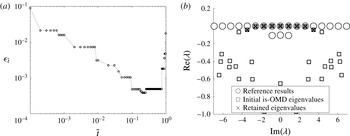
Using the eigenvalues obtained previously, the is-OMD modes of the system (4.1) are obtained from (4.8) for a Vandermonde matrix conditioned with
 $\tilde{t}=0.01$
. Figure 4 shows modes corresponding to identified eigenvalues, which accurately match the prescribed spatial wavenumbers
 $k_{1}$
and
 $k_{2}$
. Note the difference between the columns of
 $\unicode[STIX]{x1D647}$
in figure 4, where there is a visible interaction between both wavenumbers, a phenomenon which is not evident in
 $\unicode[STIX]{x1D731}^{is\text{-}OMD}$
. Although
 $\unicode[STIX]{x1D647}$
is not used in the calculation of
 $\unicode[STIX]{x1D731}^{is\text{-}OMD}$
, its inclusion in the variable space of algorithm 1 allows for greater freedom in the estimation, which may lead to more accurate
 $\unicode[STIX]{x1D706}_{i}$
and, hence, more accurate dynamical modes.
4.2 Intermediate snapshot reconstruction
Despite the fact that the intermediate snapshot variables
 $w_{i}$
in algorithm 1 provide the freedom with which accurate spectral information can be obtained, these variables typically contain high-frequency content not present in the reference data. However, using the eigenvalues
 $\unicode[STIX]{x1D726}^{is\text{-}OMD}=[\unicode[STIX]{x1D706}_{1},\ldots ,\unicode[STIX]{x1D706}_{n}]$
and dynamic modes
 $\unicode[STIX]{x1D731}^{is\text{-}OMD}=[\unicode[STIX]{x1D731}_{1},\ldots ,\unicode[STIX]{x1D731}_{n}]$
obtained from algorithm 2, it is possible to obtain an improved approximation of intermediate snapshots corresponding to time steps
 $i\notin {\mathcal{J}}$
.
To do this, consider the interpretation of the modal decomposition output described through (4.5). At each of the known analysis data snapshots
 $(\boldsymbol{u}_{k})_{k\in {\mathcal{J}}}$
we consider the projection
 $(\unicode[STIX]{x1D731}^{is\text{-}OMD})^{\text{T}}\boldsymbol{u}_{k}=:(a_{j})_{j=1}^{r}\in \mathbb{R}^{r}$
and subsequently extrapolate via
 $$\begin{eqnarray}\tilde{\boldsymbol{w}}_{i}=\mathop{\sum }_{j=1}^{n}\unicode[STIX]{x1D706}_{j}^{i}a_{j}\unicode[STIX]{x1D731}_{j},\quad k=1,\ldots ,n_{k}-1,\end{eqnarray}$$
where
 $n_{k}$
is the number of minimal time steps
 $\unicode[STIX]{x1D6FF}t$
between successive snapshots
 $\boldsymbol{u}_{k}$
and
 $\boldsymbol{u}_{k+1}$
.
The above technique is applied to the system (4.1) with the same parameters as in § 4.1, with eigenvalues
 $\unicode[STIX]{x1D706}_{j}$
and dynamic modes
 $\unicode[STIX]{x1D731}_{j}$
obtained with algorithm 2, to produce intermediate snapshots
 $\tilde{\boldsymbol{w}}_{i}$
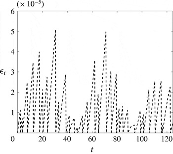
. Figure 5 presents the temporal evolution of the snapshot error
 $\unicode[STIX]{x1D716}_{i}=\Vert \tilde{\boldsymbol{w}}_{i}-\boldsymbol{w}_{i}^{ref}\Vert ^{2}/\Vert \boldsymbol{w}_{i}^{ref}\Vert ^{2}$
, where it can be seen that due to the linear nature of the system, the error increases linearly when
 $\tilde{\boldsymbol{w}}_{i}$
is estimated further away from known snapshots
 $\boldsymbol{u}_{i}$
. However, since the eigenvalues
 $\unicode[STIX]{x1D706}$
are estimated accurately, snapshot extrapolation gives a small error
 $\unicode[STIX]{x1D716}_{i}<10^{-4}$
.
Temporal evolution of the snapshots reconstruction error
 $\unicode[STIX]{x1D716}_{i}=\Vert \tilde{\boldsymbol{w}}_{i}-\boldsymbol{w}_{i}^{ref}\Vert ^{2}/\Vert \boldsymbol{w}_{i}^{ref}\Vert ^{2}$
, where
 $\tilde{\boldsymbol{w}}_{i}$
is defined by (4.10).

5 A comparison with compressive sampling
The statistical performance of both is-OMD and compressive sampling in terms of the ability to extract frequency content from undersampled data will be analysed on the one-dimensional synthetic sinusoidal flow
 $$\begin{eqnarray}f(\boldsymbol{x},t)=\mathop{\sum }_{j}A_{j}\sin (k_{j}\boldsymbol{x}+\unicode[STIX]{x1D714}_{j}t),\quad 0\leqslant \boldsymbol{x}\leqslant 1,t>0,\end{eqnarray}$$
with amplitudes
 $A_{j}>0$
, frequencies
 $\unicode[STIX]{x1D714}_{j}>0$
and wavenumbers
 $k_{j}>0$
. Similarly to the system in § 4, reference data set
 ${\mathcal{W}}=\{\boldsymbol{w}_{i}\}_{i=1}^{900}$
is generated where each snapshot
 $$\begin{eqnarray}\boldsymbol{w}_{i}=\left(f\left(\frac{j}{N},\text{i}\unicode[STIX]{x1D6FF}t\right)\right)_{j=0}^{N_{x}},\quad 0=1,\ldots ,900,\end{eqnarray}$$
is sampled at
 $N_{x}=10^{4}$
equally spaced points in
 $0\leqslant \boldsymbol{x}\leqslant 1$
. Algorithm 1 will be compared with the compressive sampling approach developed in Tu et al. (Reference Tu, Rowley, Kutz and Shang2014), which will be referred to here as CS-DMD. CS-DMD is implemented by first obtaining an approximation of the fully resolved data set,
 ${\mathcal{W}}$
, from the analysis data set
 ${\mathcal{U}}$
using a CoSaMP algorithm (Needell & Tropp Reference Needell and Tropp2009). Subsequently, the DMD eigenvalues corresponding to
 ${\mathcal{W}}$
are obtained. Accuracy is described by the proportional error in extracted frequency
 $$\begin{eqnarray}\unicode[STIX]{x1D716}_{\unicode[STIX]{x1D706}}:=\frac{|\unicode[STIX]{x1D714}_{j}-\text{Im}(\unicode[STIX]{x1D706})|}{\unicode[STIX]{x1D714}_{j}},\end{eqnarray}$$
where
 $\unicode[STIX]{x1D706}$
are the eigenvalues obtained by each of the two methods.
5.1 Robustness of CS-DMD and is-OMD
We consider data sampled from (5.1) in the case of two frequencies
 $\unicode[STIX]{x1D714}_{1}=\unicode[STIX]{x03C0}/20,\unicode[STIX]{x1D714}_{2}=2\unicode[STIX]{x03C0}/25$
, with respective amplitudes
 $A_{1}=1,A_{2}=0.5$
, and minimal time step
 $\unicode[STIX]{x1D6FF}t=1$
. The analysis data ensemble
 ${\mathcal{U}}$
is selected with an average sampling time step satisfying
 $$\begin{eqnarray}\frac{\unicode[STIX]{x0394}t_{av}}{\unicode[STIX]{x1D6FF}t_{1}^{\ast }}=\frac{7}{8},\quad \frac{\unicode[STIX]{x0394}t_{av}}{\unicode[STIX]{x1D6FF}t_{2}^{\ast }}=\frac{6}{5},\end{eqnarray}$$
as in § 4.
The first step of CS-DMD is to apply compressive sampling to
 ${\mathcal{U}}$
to form an approximation
 $\hat{{\mathcal{W}}}$
to the fully resolved data ensemble
 ${\mathcal{W}}$
. Recall from § 2.2 that this is achieved by (i) choosing and fixing a temporal basis
 $\unicode[STIX]{x1D729}$
, then (ii) successively adding a number,
 $k$
say, of elements of this basis which best correlate with the available data. Motivated by the fact that the underlying data sampled from (5.1) are sparse in the Fourier basis, we set
 $\unicode[STIX]{x1D729}$
to be the inverse Fourier Transform and obtain approximations
 $\hat{{\mathcal{W}}}_{k}\approx {\mathcal{W}}$
corresponding to extracting
 $k=4,8$
and
 $20$
dominant basis vectors. DMD is then applied to each
 $\hat{{\mathcal{W}}}_{k}$
to determine the identified eigenvalue information.
Since we do not want to assume a priori the number of dynamically important structures present in a given data set, it is desirable that the accuracy of the frequency information provided by CS-DMD behaves predictably with the requested number of basis elements
 $k$
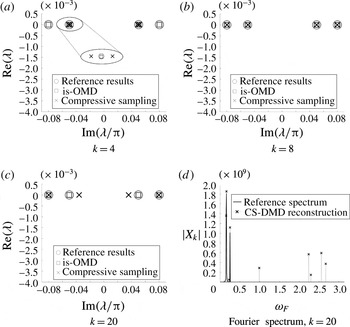
. Figure 6 indicates that this is not the case. Indeed, the frequencies
 $\unicode[STIX]{x1D714}_{i}$
are accurately identified only in the case
 $k=8$
, with
 $k=4$
failing to identify the higher frequency
 $\unicode[STIX]{x1D714}_{2}$
, while the choice
 $k=20$
results in an underapproximation of
 $\unicode[STIX]{x1D714}_{1}$
.
For
 $k=4$
, inaccuracy arises from the discrete Fourier frequencies implied by the chosen basis
 $\unicode[STIX]{x1D729}$
. Since the fully resolved data ensemble contains
 $900$
samples, the chosen basis contains only discrete frequencies
 $\unicode[STIX]{x1D714}_{F}=(2\unicode[STIX]{x03C0}n/900)_{n=0}^{900}$
,
 $k$
of which are used to express the data. For this particular example, no single
 $\unicode[STIX]{x1D714}_{F}$
coincides with
 $\unicode[STIX]{x1D714}_{1}=\unicode[STIX]{x03C0}/20$
. Instead there are multiple values of
 $\unicode[STIX]{x1D714}_{F}$
in a small neighbourhood of
 $\unicode[STIX]{x1D714}_{1}$
and, since
 $A_{1}>A_{2}$
, the CoSamp algorithm applied with
 $k=4$
(incorrectly) identifies a pair of frequencies
 $\unicode[STIX]{x1D714}_{F}$
close to
 $\unicode[STIX]{x1D714}_{1}$
. The result is improved for
 $k=8$
, which is sufficiently large to resolve both
 $\unicode[STIX]{x1D714}_{1}$
and the higher frequency
 $\unicode[STIX]{x1D714}_{2}$
. However, for
 $k=20$
it is shown in figure 6(d) that compressive sampling identifies Fourier frequencies
 $\unicode[STIX]{x1D714}_{F}$
not present in the underlying system, in addition to those close to the true values
 $\unicode[STIX]{x1D714}/\unicode[STIX]{x03C0}=0.05,0.08$
. Upon application of DMD to
 ${\mathcal{W}}_{k}$
, these extra frequencies result in an incorrect identification of
 $\unicode[STIX]{x1D714}_{1}$
.
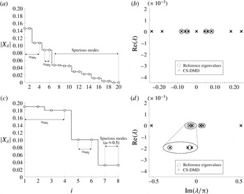
The DMD eigenvalue lattice obtained using snapshots reconstructed with CS-DMD for different numbers of sparse structures (a–c), with
 $\unicode[STIX]{x1D706}_{is\text{-}OMD}$
, is given for
 $r=45$
. The Fourier spectrum obtained by compressive sampling for
 $k=20$
is shown in (d).

Such a lack of robustness with respect to
 $k$
is not evident in the application of algorithm 1 to this example, which, as can be seen in figure 6(a–c), correctly identifies the two underlying frequencies in the data using a model of order
 $r=45$
. The is-OMD results in figure 6(a–c) present only four eigenvalues of interest. The eigenvalues of relevance were chosen based on the energetic criterion similar to approaches in Rowley et al. (Reference Rowley, Mezic, Bagheri, Schlatter and Henningson2009), Chen et al. (Reference Chen, Tu and Rowley2012), Jovanovic et al. (Reference Jovanovic, Schmid and Nichols2014), where the magnitudes of the DMD modes are examined. Here, the magnitude of a solution to (4.8),
 $\Vert \unicode[STIX]{x1D731}_{k}\Vert _{2}$
, is assessed and eigenvalues with the largest magnitude of the associated modes are selected. Note that, if
 $\unicode[STIX]{x1D651}_{{\mathcal{J}}}$
contains dynamically unimportant eigenvalues with large decay rate, the associated modes will have an excessively large magnitude in order to compensate for the low value of
 $\unicode[STIX]{x1D706}_{j}^{i-1}$
at later time steps. Therefore, in order to obtain a meaningful ranking of modes based on the energy criterion, it is important to remove dynamically unimportant rows of
 $\unicode[STIX]{x1D651}_{{\mathcal{J}}}$
using algorithm 2. Here, (4.8) is solved using
 $\unicode[STIX]{x1D651}_{{\mathcal{J}}}$
conditioned with
 $\tilde{t}=10^{-3}$
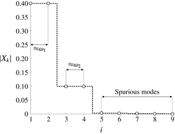
retaining nine rows of Vandermonde matrix, and consequently nine structures. Figure 7 shows a relative energetic contribution of each mode to the system dynamics defined as
 $|X_{k}|=\Vert \unicode[STIX]{x1D731}_{k}\Vert _{2}/\!\sum _{j}\Vert \unicode[STIX]{x1D731}_{k}\Vert _{2}$
, demonstrating a clearly visible drop in
 $\Vert \tilde{\unicode[STIX]{x1D731}}_{k}\Vert _{2}$
between dynamically important and unimportant eigenvalues and allowing the identification of frequencies presented in figure 6(a–c).
The relative contribution of the is-OMD modes.

Note that another variable prescribed a priori in the CS-DMD methodology is the rank
 $r$
of the DMD approximation, which is upper bounded by the number of extracted basis vectors
 $k$
. The CS-DMD results presented in figure 6 were obtained with DMD approximation of rank
 $r=4$
as opposed to
 $r=45$
of the is-OMD results. The reason for selecting this rank for the CS-DMD approximation can be explained if the maximal case
 $r=k$
is instead considered. With this choice, DMD eigenvalue information will replicate the Fourier frequencies which most accurately correlate with the analysis data ensemble,
 ${\mathcal{U}}$
. Figure 8(a) presents the relative contribution of each mode for
 $r=k=20$
. Although the frequencies corresponding to the most dominant modes are close to the true values, it is nonetheless not clear from figure 8(a) how to choose a threshold which will allow frequencies of dynamical importance to be retained. A similar situation occurs in figure 8(c) for
 $r=k=8$
.
For
 $r=k=8$
eigenvalues coincide with
 $\unicode[STIX]{x1D714}_{F}$
which lie in a small neighbourhood of
 $\unicode[STIX]{x1D714}_{1}$
and
 $\unicode[STIX]{x1D714}_{2}$
with a small error
 $\unicode[STIX]{x1D716}_{\unicode[STIX]{x1D706}}$
corresponding to those frequencies. However, it is shown in figure 6(b) that if a combination
 $k=8,r=4$
is used,
 $\unicode[STIX]{x1D716}_{\unicode[STIX]{x1D706}}$
decreases further. Based on these observations, in § 5.2 where a statistical sample of sinusoidal flows is investigated, for CS-DMD methodology a combination of
 $k=8$
and
 $r=4$
is utilised.
The output of the CS-DMD methodology for different values of
 $k$
and
 $r$
where
 $k=r$
. The importance of modes and corresponding eigenvalue spectrum for
 $k=r=20$
is shown in (a,b) while those corresponding to
 $k=r=8$
are presented in (c,d).

5.2 Frequency estimation analysis: statistical comparison between compressive sampling and is-OMD
To study the differences in performance of is-OMD and compressive sampling, both methodologies were applied to the system (5.1) for a range of frequencies and average sampling rates. In particular, the lower frequency is fixed, as above, to
 $\unicode[STIX]{x1D714}_{1}=\unicode[STIX]{x03C0}/20$
, while the higher system frequency takes one of values
 $$\begin{eqnarray}\unicode[STIX]{x1D714}_{2}(n)=\unicode[STIX]{x1D714}_{1}+\frac{n\unicode[STIX]{x03C0}}{100},\quad n=1,\ldots ,20.\end{eqnarray}$$
Subsequently, for each of value of
 $\unicode[STIX]{x1D714}_{2}(n)$
a number of downsampled analysis data ensembles
 ${\mathcal{U}}_{nm}$
are constructed whose average sampling rates satisfy
 $$\begin{eqnarray}\frac{\unicode[STIX]{x0394}t_{av}({\mathcal{U}}_{nm})}{\unicode[STIX]{x1D6FF}t_{2}^{\ast }}=1+\frac{m}{20},\quad m=1,\ldots ,55,\end{eqnarray}$$
that is, each exceeds the Nyquist criterion to differing degrees. This is achieved by constructing fully resolved data sets
 $$\begin{eqnarray}{\mathcal{W}}_{nm}=\left\{f\left(\boldsymbol{x},i\left(\frac{1+m/20}{1+n/5}\right)\right):0\leqslant \boldsymbol{x}\leqslant 1,\;i=1,\ldots ,900\right\}\end{eqnarray}$$
and sampling non-uniform analysis data ensembles
 ${\mathcal{U}}_{nm}\subset {\mathcal{W}}_{nm}$
, each of cardinality
 $|{\mathcal{U}}_{nm}|=45$
. Note that the fully resolved data set is varied for each pair
 $(n,m)$
in order that analysis data sets with different average downsampling rates (as a proportion of
 $\unicode[STIX]{x1D6FF}t_{2}^{\ast }$
) can be constructed to possess the same proportion, 5 %, of elements to the fully resolved ensemble.
The CS-DMD and is-OMD algorithms are applied to each data set
 ${\mathcal{U}}_{nm}$
. Motivated by § 5, we apply the CoSamp algorithm with sparse basis matrix
 $\unicode[STIX]{x1D729}$
as the inverse Fourier transform and set the sparsity level to
 $k=8$
. Algorithm 1 is initialised with
 $(\unicode[STIX]{x1D648}_{0})_{ij}=N(0,\unicode[STIX]{x1D70E}^{2})+\unicode[STIX]{x1D6FF}_{ij}$
, that is, a small perturbation of the identity matrix with
 $\unicode[STIX]{x1D70E}=\sqrt{0.3}$
, and
 $\unicode[STIX]{x1D647}_{0}=\text{POD}({\mathcal{U}}_{nm})$
, with the modelling dimension set as
 $r=|{\mathcal{U}}_{nm}|=45$
.
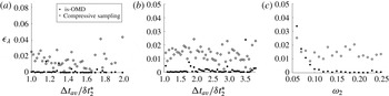
Figures 9(a) and 9(b) show the proportional frequency error
 $\unicode[STIX]{x1D716}_{\unicode[STIX]{x1D706}}$
corresponding to
 $\unicode[STIX]{x1D714}_{1},\unicode[STIX]{x1D714}_{2}$
, respectively, averaged over the different values of
 $\unicode[STIX]{x0394}t_{av}({\mathcal{U}}_{nm})/\unicode[STIX]{x1D6FF}t_{2}^{\ast }$
. Note that, since the data are sampled in such a way to achieve a particular value of
 $\unicode[STIX]{x0394}t_{av}/\unicode[STIX]{x1D6FF}t_{2}^{\ast }$
, the corresponding downsampling ratio for
 $\unicode[STIX]{x1D6FF}t_{1}^{\ast }$
is
 $\unicode[STIX]{x0394}t_{av}/\unicode[STIX]{x1D6FF}t_{1}^{\ast }=(\unicode[STIX]{x0394}t_{av}/\unicode[STIX]{x1D6FF}t_{2}^{\ast })(\unicode[STIX]{x1D714}_{1}/\unicode[STIX]{x1D714}_{2})$
, meaning that
 $\unicode[STIX]{x0394}t_{av}/\unicode[STIX]{x1D6FF}t_{1}^{\ast }$
are not similarly grouped. Consequently, a discrete set of values is defined,
 ${\mathcal{S}}=\{1.02,1.04,\ldots ,1.92\}$
, and for each element
 ${\mathcal{S}}_{i}$
results satisfying
 $|\unicode[STIX]{x0394}t_{av}/\unicode[STIX]{x1D6FF}t_{1}^{\ast }-{\mathcal{S}}_{i}|<0.01$
are grouped together and averaged accordingly. It is clear from figure 9(a,b) that the proportional frequency error is reduced by application of algorithm 1 in comparison to CS-DMD.
Average proportional frequency error
 $\unicode[STIX]{x1D716}_{\unicode[STIX]{x1D706}}$
corresponding to
 $\unicode[STIX]{x1D714}_{1}$
(a) and
 $\unicode[STIX]{x1D714}_{2}$
(b) for each
 $\unicode[STIX]{x0394}t_{av}/\unicode[STIX]{x1D6FF}_{2}^{\ast }$
; and corresponding to each
 $\unicode[STIX]{x1D714}_{2}$
when
 $\unicode[STIX]{x1D716}_{\unicode[STIX]{x1D706}}$
is averaged over a range of different downsampling ratios
 $\unicode[STIX]{x0394}t_{av}/\unicode[STIX]{x1D6FF}_{2}^{\ast }$
(c).

Figure 9(c) shows the proportional frequency error
 $\unicode[STIX]{x1D716}_{\unicode[STIX]{x1D706}}$
corresponding to
 $\unicode[STIX]{x1D714}_{2}$
, as
 $\unicode[STIX]{x1D714}_{2}$
is varied, each averaged over the
 $55$
different values of the downsampling ratio
 $\unicode[STIX]{x0394}t_{av}/\unicode[STIX]{x1D6FF}t_{2}^{\ast }$
. The CS-DMD error is approximately constant, while to is-OMD error decays as
 $|\unicode[STIX]{x1D714}_{1}-\unicode[STIX]{x1D714}_{2}|$
increases. It should be noted that such a pattern can be observed if the OMD algorithm is applied to fully time-resolved snapshots
 ${\mathcal{W}}$
which contain observation noise. This is, pairs of eigenvalues satisfying
 $|\text{Im}(\unicode[STIX]{x1D706}_{i})-\text{Im}(\unicode[STIX]{x1D706}_{j})|\ll 1$
are sensitive to observation noise.
6 Numerical example: cylinder wake
Algorithms 1 and 2 are applied to the numerical results of the circular cylinder flow at
 $\mathit{Re}=60$
and their performance is analysed on the limit cycle regime. The numerical data were obtained using the in-house solver called Pantarhei, which was validated for the cylinder flow in Lu & Papadakis (Reference Lu and Papadakis2011, Reference Lu and Papadakis2014). The code uses the finite volume method in an unstructured grid. The spatial terms of Navier–Stokes equations were discretised using a second-order central scheme and the system was advanced in time using a second-order, three-point backward scheme. The domain used for the simulations was 48
 $D$
long and 32
 $D$
wide, where
 $D$
is the cylinder diameter. The distance between cylinder location and upstream and downstream boundaries is respectively 16
 $D$
and 32
 $D$
. The total number of cells was 62 791. The grid was non-uniform with the minimum grid spacing
 $h\approx D/60$
near the cylinder boundary. Uniform inflow (
 $U_{\infty }=1$
), convective outflow and symmetric boundary conditions on the lateral sides of the domain were imposed. Additionally, a no-slip condition was imposed on the cylinder boundary. Density and viscosity of the flow were modified accordingly to achieve the desired Reynolds number. This dynamical system exhibits a pair of vortices oscillating at a shedding frequency together with the series of higher harmonics; each oscillating at an integer multiple of the shedding frequency. These values can be extracted by applying the OMD algorithm to time-resolved data.
The performance of is-OMD will be assessed by comparing the eigenvalue information between eigenvalues retained in the post-processing algorithm 2,
 $\unicode[STIX]{x1D726}^{is\text{-}OMD}$
, and
 $\unicode[STIX]{x1D706}_{OMD}$
from the OMD algorithm applied to time-resolved data. Three aspects of algorithm initialisation and their impact on the extraction of dynamic information are discussed here: the initialisation of
 $\unicode[STIX]{x1D647}_{0}$
and
 $\unicode[STIX]{x1D648}_{0}$
; the projection rank
 $r$
; and sampling strategy
 ${\mathcal{J}}$
. A downsampled data set
 ${\mathcal{U}}$
is extracted randomly from a reference data set
 ${\mathcal{W}}$
uniformly sampled at
 $\unicode[STIX]{x1D6FF}t=0.25s$
containing 30 snapshots per shedding period. Here, it is convenient to introduce the following quantities related to the sampling strategy:
 $\unicode[STIX]{x0394}t_{av}=\sum _{i\in {\mathcal{J}}}\unicode[STIX]{x0394}t_{i}/|{\mathcal{J}}|$
,
 $\unicode[STIX]{x0394}t_{min}=\min \{\unicode[STIX]{x0394}t_{i}\;|\;i\in {\mathcal{J}}\}$
and
 $\unicode[STIX]{x0394}t_{max}=\max \{\unicode[STIX]{x0394}t_{i}\;|\;i\in {\mathcal{J}}\}$
. Unless stated otherwise,
 ${\mathcal{U}}$
is sampled such that
 $\unicode[STIX]{x0394}t_{av}=10\unicode[STIX]{x1D6FF}t$
without constraints on
 $\unicode[STIX]{x0394}t_{min}$
and
 $\unicode[STIX]{x0394}t_{max}$
. Applying a Nyquist criterion to data downsampled at a constant
 $\unicode[STIX]{x0394}t=10\unicode[STIX]{x1D6FF}t$
, such downsampling is sufficient to resolve the vortex-shedding frequency but not satisfactory if the objective is to identify higher-frequency modes.
6.1 Initial condition analysis
To assess the most appropriate properties of
 $\unicode[STIX]{x1D647}_{0}$
and
 $\unicode[STIX]{x1D648}_{0}$
to initialise is-OMD, three classes of initial condition are considered:
-
(i)
 $\unicode[STIX]{x1D647}_{0}$
is set to POD modes of the known data,
$\unicode[STIX]{x1D650}$
, and an identity matrix chosen to approximate
$\unicode[STIX]{x1D648}_{0}$
, i.e.
$\unicode[STIX]{x1D647}_{0}=\text{POD}(\unicode[STIX]{x1D650})$
,
$\unicode[STIX]{x1D648}_{0}=\unicode[STIX]{x1D644}_{r}$
;
-
(ii)
$\unicode[STIX]{x1D647}_{0}=\text{POD}(\unicode[STIX]{x1D650})$
and an identity matrix with entries perturbed by noise used for
$\unicode[STIX]{x1D648}_{0}$
:
$(\unicode[STIX]{x1D648}_{0})_{ij}=N(0,\unicode[STIX]{x1D70E})+\unicode[STIX]{x1D6FF}_{ij}$
; -
(iii) OMD is applied to data undersampled with a constant time step
$\unicode[STIX]{x0394}t$
,
$\overline{\unicode[STIX]{x1D650}}$
, to obtain
$\unicode[STIX]{x1D647}_{0}$
and
$\unicode[STIX]{x1D648}_{0}$
, i.e.
$[\unicode[STIX]{x1D648}_{0},\unicode[STIX]{x1D647}_{0}]=\text{OMD}(\overline{\unicode[STIX]{x1D650}})$
.






The motivation for
 $[\unicode[STIX]{x1D648}_{0},\unicode[STIX]{x1D647}_{0}]=\text{OMD}(\overline{\unicode[STIX]{x1D650}})$
is that in systems exhibiting limit cycle behaviour, their dynamics does not qualitatively change with time. In such a case, two sets of data can be acquired, one with non-uniform
 $\unicode[STIX]{x0394}t$
which is used as an input to is-OMD,
 $\unicode[STIX]{x1D650}$
, and a second one which is uniformly subsampled,
 $\overline{\unicode[STIX]{x1D650}}$
. In such a case
 $\overline{\unicode[STIX]{x1D650}}$
is not sufficient to obtain all the dynamics of interest; however, the output of OMD can still be used for
 $\unicode[STIX]{x1D647}_{0}$
and
 $\unicode[STIX]{x1D648}_{0}$
.
In order to consider the role of the initial conditions, the same downsampling strategy and approximation rank
 $r$
are used for all three cases. In particular,
 ${\mathcal{U}}$
is sampled non-uniformly, with
 $\unicode[STIX]{x0394}t_{av}=10\unicode[STIX]{x1D6FF}t$
and without constraints on
 $\unicode[STIX]{x0394}t_{min}$
and
 $\unicode[STIX]{x0394}t_{max}$
, while the projection rank is set to
 $r=75$
. The dimensions of both data sets
 ${\mathcal{W}}$
,
 ${\mathcal{U}}$
are
 $\unicode[STIX]{x1D652}\in \mathbb{R}^{p\times 750}$
,
 $\unicode[STIX]{x1D650}\in \mathbb{R}^{p\times 75}$
, i.e.
 $|{\mathcal{I}}|=750$
and
 $|{\mathcal{J}}|=75$
. The
 $\overline{\unicode[STIX]{x1D650}}\in \mathbb{R}^{p\times 75}$
was sampled such that
 $\unicode[STIX]{x0394}t_{av}=10\unicode[STIX]{x1D6FF}t$
, which is sufficient to resolve a time scale of
 $2/3T$
, where
 $T$
is a shedding frequency. Note that cylinder flow contains harmonics with time scales of
 $T/n$
for
 $n\in \mathbb{Z}^{+}$
, meaning that
 $2/3T$
is not sufficient to resolve the subharmonic with a time scale of
 $T/2$
.
The extracted dynamical information for
 $\unicode[STIX]{x1D648}_{0}=\unicode[STIX]{x1D644}_{r}$
,
 $[\unicode[STIX]{x1D648}_{0},\unicode[STIX]{x1D647}_{0}]=\text{OMD}(\overline{\unicode[STIX]{x1D650}})$
and
 $(\unicode[STIX]{x1D648}_{0})_{ij}=N(0,\unicode[STIX]{x1D70E})+\unicode[STIX]{x1D6FF}_{ij}$
with
 $\unicode[STIX]{x1D70E}=10^{-2},10^{-3}$
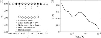
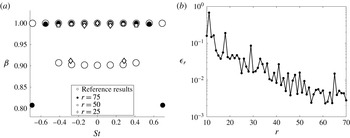
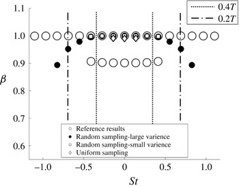
are presented in figure 10. In all of the analysed cases, only the eigenvalues retained in algorithm 2 for
 $\tilde{t}=0.3$
are presented. The Strouhal number is defined as
 $St=fD/U_{\infty }$
, where
 $D$
is the cylinder diameter and
 $U_{\infty }$
is the inflow velocity. Assuming that flow field was non-dimensionalised using a cylinder diameter and an inflow velocity, the Strouhal number can be extracted from the phase information of each eigenvalue,
 $St=\text{Im}(\unicode[STIX]{x1D706})/(2\unicode[STIX]{x03C0})$
. The magnitude of the eigenvalue provides the information about the growth rate, which is expressed in such a way so that growth rate,
 $\unicode[STIX]{x1D6FD}$
, follows
 $\unicode[STIX]{x1D6FD}^{t}$
, i.e.
 $\unicode[STIX]{x1D6FD}=\exp (\text{Re}(\unicode[STIX]{x1D706}))$
. The reference eigenvalues in figure 10 were obtained by applying the OMD algorithm to
 $\unicode[STIX]{x1D652}$
for
 $r=30$
, and consist of the asymptotic eigenvalues representing the limit cycle behaviour and eigenvalues at
 $\unicode[STIX]{x1D6FD}=0.9$
characterising relaxation of the flow onto its limit cycle (Bagheri Reference Bagheri2013). The primary objective is to assess the accuracy at which the is-OMD algorithm approximates the asymptotic eigenvalues, since the values at
 $\unicode[STIX]{x1D6FD}=0.9$
correspond to dynamics at extremely low energy for the chosen data set
 $\unicode[STIX]{x1D652}$
.
Eigenvalues of the dynamic matrix
 $\unicode[STIX]{x1D648}$
obtained using the is-OMD algorithm for different initial conditions (a). The error in eigenvalue magnitude for identity matrices with
 $\unicode[STIX]{x1D748}\in [10^{-9},10^{-2}]$
(b), obtained for the projection rank
 $r=75$
.

In the case where
 $\unicode[STIX]{x1D648}_{0}=\unicode[STIX]{x1D644}_{r}$
, a majority of the eigenvalues of
 $\unicode[STIX]{x1D648}$
are characterised by
 $\text{Re}(\unicode[STIX]{x1D706})\ll 0$
and are discarded in algorithm 2 due to the choice of
 $\tilde{t}$
. None of the frequencies present in the system are recovered. For
 $[\unicode[STIX]{x1D648}_{0},\unicode[STIX]{x1D647}_{0}]=\text{OMD}(\overline{\unicode[STIX]{x1D650}})$
, only frequencies within time-scale range of
 $\overline{\unicode[STIX]{x1D650}}$
are correctly estimated (i.e.
 $St\in [-0.2,0.2]$
). Figure 10 demonstrates that noise must be added to
 $\unicode[STIX]{x1D648}_{0}$
in order to extract high-frequency harmonics. It is interesting to note that as the standard deviation increases, more frequency information is recovered. In particular, for an order of magnitude increase in
 $\unicode[STIX]{x1D70E}$
, an additional conjugate pair of eigenvalues is correctly identified and the growth rate of all eigenvalues,
 $\unicode[STIX]{x1D6FD}$
, is more accurate.
In order to further demonstrate a beneficial influence of noise addition, a repeated analysis was performed for
 $(\unicode[STIX]{x1D648}_{0})_{ij}=N(0,\unicode[STIX]{x1D70E})+\unicode[STIX]{x1D6FF}_{ij}$
with
 $\unicode[STIX]{x1D70E}\in [10^{-9},10^{-2}]$
. Accuracy in the estimation of seven most dominant eigenvalues is analysed and the proportional error is defined as
 $\unicode[STIX]{x1D716}:=\sum _{i=1}^{7}|\unicode[STIX]{x1D706}_{i}^{true}-\unicode[STIX]{x1D706}_{i}^{is\text{-}OMD}|/\sum _{i=1}^{7}|\unicode[STIX]{x1D706}_{i}^{true}|$
. Figure 10 demonstrates that
 $\unicode[STIX]{x1D716}$
decreases as
 $\unicode[STIX]{x1D70E}$
increases. It is clear that, in order for the is-OMD algorithm to successfully recover dynamical information, a certain degree of flexibility has to be included in
 $\unicode[STIX]{x1D648}_{0}$
. For
 $\unicode[STIX]{x1D648}_{0}=\unicode[STIX]{x1D644}_{r}$
and
 $[\unicode[STIX]{x1D648}_{0},\unicode[STIX]{x1D647}_{0}]=\text{OMD}(\overline{\unicode[STIX]{x1D650}})$
, the dynamics corresponding to dominant structures present in the system, i.e. constant mean mode and shedding vortices, are strongly embedded in the initial matrix structure. In such cases the objective function can be significantly reduced in few iterations, indicating that such a
 $\unicode[STIX]{x1D648}_{0}$
predetermines a local minimum of (2.10). This problem appears to be avoided simply by randomly perturbing the initial matrices. Note that it is possible to adjust a frequency range of the eigenvalue spectrum of
 $(\unicode[STIX]{x1D648}_{0})_{ij}=N(0,\unicode[STIX]{x1D70E})+\unicode[STIX]{x1D6FF}_{ij}$
by adjusting a value of
 $\unicode[STIX]{x1D70E}$
, where larger value of
 $\unicode[STIX]{x1D70E}$
will cover larger range of frequencies. If the system exhibits primarily low-frequency dynamics it is desirable to set
 $\unicode[STIX]{x1D70E}$
to a lower value such that an eigenvalue spectrum of
 $\unicode[STIX]{x1D648}_{0}$
is in a neighbourhood of the expected range of the frequencies of interest.
6.2 Rank size analysis
It was demonstrated in § 5.1 that setting a high value of
 $k$
in the CS-DMD approach induces Fourier modes corresponding to high-frequency oscillations not present in time-resolved data. It is therefore important to consider the impact of the equivalent parameter in the is-OMD algorithm, that is, the dimension
 $r$
of
 $\text{Im}(\unicode[STIX]{x1D647})$
. It will be demonstrated here that larger
 $r$
improves accuracy in the recovered eigenvalues, which consequently leads to an improved accuracy of
 $\unicode[STIX]{x1D731}^{is\text{-}OMD}$
in algorithm 2. An analysis in terms of the eigenvalue and mode estimation is performed for
 $r=[25,50,75]$
using the same sampling strategy as in § 6.1 and setting
 $(\unicode[STIX]{x1D648}_{0})_{ij}=N(0,0.3)+\unicode[STIX]{x1D6FF}_{ij}$
,
 $\unicode[STIX]{x1D647}_{0}=\text{POD}(\unicode[STIX]{x1D650})$
.
Figure 11 presents eigenvalue lattices for different values of
 $r$
and demonstrates a positive impact of increasing
 $r$
on the accuracy of the dynamic estimation. When
 $r$
increases, a progressively greater number of asymptotic eigenvalues is recovered and their growth rates
 $\unicode[STIX]{x1D6FD}$
converge towards the correct value of 1. The number of modes which can be calculated is proportional to the number of recovered eigenvalues. For
 $r$
of 25, 50 and 75 there are respectively one, three and four conjugate pairs of eigenvalues that are estimated with small error, and with growth rate
 $\unicode[STIX]{x1D6FD}>0.95$
. The dynamic modes are estimated as a solution to (4.8) which in turn depends upon
 $\unicode[STIX]{x1D651}_{{\mathcal{J}}}$
being constructed using accurate eigenvalues. Figure 13 shows dynamic modes corresponding to eigenvalues with
 $\unicode[STIX]{x1D6FD}>0.95$
obtained for
 $r=75$
, and it demonstrates that the mode shapes closely resemble the coherent structures obtained from time-resolved data (figure 12). The dynamic modes of similar precision can be obtained for other eigenvalues presented in 11, where
 $\unicode[STIX]{x1D6FD}>0.95$
, therefore mode shapes for
 $r=25$
and
 $r=50$
are omitted here.
Note that for
 $r=25$
and
 $r=75$
a pair of eigenvalues is recovered which contains an error in
 $\unicode[STIX]{x1D6FD}$
. Figure 14 shows the corresponding dynamic modes. Although these structures are not as coherent as for eigenvalues where
 $\unicode[STIX]{x1D6FD}>0.95$
, there is nonetheless a resemblance to the structures present in the flow (figure 12). It is expected that when
 $r$
is increased even further the eigenvalue accuracy improves, leading to better precision in the estimation of the dynamic modes. In practice, when
 $\unicode[STIX]{x1D647}_{0}=POD(\unicode[STIX]{x1D650})$
and
 $(\unicode[STIX]{x1D648}_{0})_{ij}=N(0,\unicode[STIX]{x1D70E})+\unicode[STIX]{x1D6FF}_{ij}$
are used,
 $r$
is only limited by
 $|{\mathcal{J}}|$
. This quantity is usually much higher than for the results presented here, and the choice of
 $r$
would be limited only by the processing cost.
Eigenvalues of the dynamic matrix
 $\unicode[STIX]{x1D648}$
for
 $r=[25,50,75]$
(a). The error
 $\unicode[STIX]{x1D716}_{r}=(1/|{\mathcal{I}}|)\sum _{i\in {\mathcal{I}}}\Vert \tilde{\unicode[STIX]{x1D652}}-\unicode[STIX]{x1D652}^{ref}\Vert ^{2}/\Vert \unicode[STIX]{x1D652}^{ref}\Vert ^{2}$
for
 $(\unicode[STIX]{x1D648}_{0})_{ij}=N(0,0.3)+\unicode[STIX]{x1D6FF}_{ij}$
with different
 $r$
(b).

Modes
 $\unicode[STIX]{x1D731}=\unicode[STIX]{x1D647}\unicode[STIX]{x1D64B}$
obtained by applying the OMD algorithm to a time-resolved cylinder flow data.

Modes
 $\unicode[STIX]{x1D731}^{is\text{-}OMD}$
corresponding to eigenvalues with
 $\unicode[STIX]{x1D6FD}>0.95$
obtained using the is-OMD algorithm for
 $r=75$
.

Modes
 $\unicode[STIX]{x1D731}^{is\text{-}OMD}$
corresponding to eigenvalues presented in figure 11 with
 $\unicode[STIX]{x1D6FD}<0.95$
;
 $St=0.28$
,
 $\unicode[STIX]{x1D6FD}=0.91$
for
 $r=25$
(a) and
 $St=0.69$
,
 $\unicode[STIX]{x1D6FD}=0.81$
for
 $r=75$
(b).

When unknown data sets are reconstructed using (4.10), the value of
 $r$
impacts the accuracy of estimated snapshots,
 $\tilde{\unicode[STIX]{x1D652}}=[\tilde{\boldsymbol{w}}_{1},\ldots ,\tilde{\boldsymbol{w}}_{N}]$
for
 $i\notin {\mathcal{J}}$
, through the precision and number of reconstructed eigenvalues
 $\unicode[STIX]{x1D706}_{j}$
and dynamic modes
 $\unicode[STIX]{x1D731}_{j}$
, and is expected to improve when
 $r$
is increased. This fact is confirmed in figure 11, which presents the evolution of the error norm,
 $\unicode[STIX]{x1D716}_{r}=(1/|{\mathcal{I}}|)\sum _{i\in {\mathcal{I}}}\Vert \tilde{\unicode[STIX]{x1D652}}-\unicode[STIX]{x1D652}^{ref}\Vert ^{2}/\Vert \unicode[STIX]{x1D652}^{ref}\Vert ^{2}$
for
 $r\in [10,70]$
. There is a visible decay in the value of
 $\unicode[STIX]{x1D716}_{r}$
, where
 $\unicode[STIX]{x1D716}_{r}$
is less than 5 % for
 $r\geqslant 30$
. Note that, despite being governed by nonlinear Navier–Stokes equations, cylinder flow in the limit cycle is known to be well approximated by a linear model consisting of oscillating structures. For more dynamically complex systems, the value of
 $\unicode[STIX]{x1D716}_{r}$
is expected to have a larger magnitude than values presented in figure 11.
Finally, we note that the accuracy of
 $\tilde{\unicode[STIX]{x1D652}}$
depends upon the value of
 $\unicode[STIX]{x1D706}_{j}$
used in (4.10). The number and choice of
 $\unicode[STIX]{x1D706}_{j}$
is determined based on the number of retained rows in
 $\unicode[STIX]{x1D651}_{{\mathcal{J}}}$
, which is conditioned with an appropriate value of
 $\tilde{t}$
. When
 $\tilde{t}$
is small, a majority of
 $\unicode[STIX]{x1D706}_{j}$
in
 $\unicode[STIX]{x1D651}_{{\mathcal{J}}}$
are retained, including dynamically unimportant values, introducing an error in
 $\tilde{\unicode[STIX]{x1D652}}$
. On the other hand, if
 $\tilde{t}$
is large, dynamically relevant
 $\unicode[STIX]{x1D706}_{j}$
are removed. In order to find an appropriate value of
 $\tilde{t}$
, and consequently number of retained
 $\unicode[STIX]{x1D706}_{j}$
, let us compare snapshots estimated using (4.10) with reference measurements. Starting an extrapolation at each
 $i\in {\mathcal{J}}$
a snapshot is estimated at the time step when the next measurements is acquired, i.e.
 $\tilde{\boldsymbol{w}}_{i+n_{i}}$
, where
 $n_{i}:=\unicode[STIX]{x0394}t_{i}/\unicode[STIX]{x1D6FF}t$
is the number of minimal time steps
 $\unicode[STIX]{x1D6FF}t$
between the next element of
 ${\mathcal{U}}$
. Performing a comparison with all of the available measurements, a proportional error metric
 $\unicode[STIX]{x1D716}_{\tilde{t}}=(1/|{\mathcal{J}}|)\sum _{i\in {\mathcal{J}}}\Vert \tilde{\boldsymbol{w}}_{i+n_{i}}-\boldsymbol{u}_{i+n_{i}}\Vert /\Vert \boldsymbol{u}_{i+n_{i}}\Vert$
is defined, and
 $\tilde{t}$
is estimated such that the resulting
 $\tilde{\boldsymbol{w}}_{i+n_{i}}$
minimises
 $\unicode[STIX]{x1D716}_{\tilde{t}}$
.
An example for the cylinder flow is-OMD results with
 $r=70$
is presented in figure 15, which shows
 $\unicode[STIX]{x1D716}_{\tilde{t}}$
for
 $\tilde{\boldsymbol{w}}_{i+n_{i}}$
estimated with
 $\tilde{t}\in [10^{-4},1]$
. For this particular case,
 $\unicode[STIX]{x1D716}_{\tilde{t}}$
is minimised at
 $\tilde{t}=0.21$
, where
 $\tilde{\unicode[STIX]{x1D652}}$
is calculated using the nine most dominant eigenvalues (figure 15). Although
 $\tilde{t}=0.21$
gives the smallest values of
 $\unicode[STIX]{x1D716}_{\tilde{t}}$
, there is a clear trough visible for
 $\tilde{t}\in [0.01,0.75]$
, and setting
 $\tilde{t}$
to any value in that range will give a good estimation of snapshots at
 $i\notin {\mathcal{J}}$
. In figure 11, each value of
 $\unicode[STIX]{x1D716}_{r}$
was obtained for
 $\tilde{\unicode[STIX]{x1D652}}$
estimated with the smallest value of
 $\tilde{t}$
.
The error
 $\unicode[STIX]{x1D716}_{\tilde{t}}=(1/|{\mathcal{J}}|)\sum _{i\in {\mathcal{J}}}\Vert \tilde{\boldsymbol{w}}_{i+n_{i}}-\boldsymbol{u}_{i+n_{i}}\Vert /\Vert \boldsymbol{u}_{i+n_{i}}\Vert$
for different
 $\tilde{t}$
(a) and retained is-OMD eigenvalue spectrum for
 $\tilde{t}=0.21$
(b).

6.3 The importance of random sampling
One of the key properties of the compressive sampling methodology, described in § 2.2, is its reliance on non-uniform sampling (Candes & Tao Reference Candes, J. and Tao2006b
). Here, it is demonstrated that is-OMD can also be improved by random sampling. Three different sampling strategies are analysed, with approximately the same
 $|{\mathcal{J}}|$
and
 $\unicode[STIX]{x0394}t_{av}$
for different
 $\unicode[STIX]{x0394}t_{min}$
and
 $\unicode[STIX]{x0394}t_{max}$
. Depending on
 $\unicode[STIX]{x0394}t_{min}$
, it is possible to use the Nyquist sampling criterion to estimate the range of different time scales that can be recovered as a multiple of shedding time scale
 $T$
. Setting
 $(\unicode[STIX]{x1D648}_{0})_{ij}=N(0,0.3)+\unicode[STIX]{x1D6FF}_{ij}$
,
 $\unicode[STIX]{x1D647}_{0}=POD(\unicode[STIX]{x1D650})$
and
 $r=70$
, is-OMD is applied to the following sampling strategies.
-
(i) Uniform sampling:
${\mathcal{U}}$
is sampled uniformly with
$\unicode[STIX]{x0394}t=10\unicode[STIX]{x1D6FF}t$
. Such a sampling strategy corresponds to three snapshots per shedding period and is sufficient to resolve time scales greater than
$2/3T$
. In particular
$|{\mathcal{J}}|=79$
and
$|{\mathcal{I}}|=781$
. -
(ii) Random sampling (large variance):
${\mathcal{U}}$
is sampled non-uniformly such that
$\unicode[STIX]{x0394}t_{min}=3\unicode[STIX]{x1D6FF}t$
(
$0.2T$
) and
$\unicode[STIX]{x0394}t_{max}=17\unicode[STIX]{x1D6FF}t$
(
$1.15T$
), which results in
$|{\mathcal{J}}|=80$
and
$|{\mathcal{I}}|=783$
. Together
$\unicode[STIX]{x0394}t_{min}$
and
$\unicode[STIX]{x0394}t_{max}$
encompass 3 % of
$|{\mathcal{J}}|$
. -
(iii) Random sampling (small variance):
${\mathcal{U}}$
is sampled non-uniformly such that
$\unicode[STIX]{x0394}t_{min}=6\unicode[STIX]{x1D6FF}t$
(
$0.4T$
) and
$\unicode[STIX]{x0394}t_{max}=14\unicode[STIX]{x1D6FF}t$
(
$0.95T$
), which results in
$|{\mathcal{J}}|=79$
and
$|{\mathcal{I}}|=783$
. Together
$\unicode[STIX]{x0394}t_{min}$
and
$\unicode[STIX]{x0394}t_{max}$
encompass 5 % of
$|{\mathcal{J}}|$
.


Figure 16 shows the eigenvalues retained using the algorithm 2 with
 $\tilde{t}=0.1$
for all three cases. Recall that the limit cycle dynamics of the cylinder flow are characterised by structures oscillating with frequency
 $n/T$
, where
 $n\in \mathbb{Z}^{+}$
, and having corresponding time scales of
 $T/n$
. For the cylinder data used at in the analysis, a uniform time step
 $\unicode[STIX]{x0394}t=10\unicode[STIX]{x1D6FF}t$
is high enough to recover
 $T$
but not sufficient to extract higher-frequency dynamics. Figure 16 shows that when the is-OMD algorithm is applied to uniformly sampled data, high-frequency dynamics are not recovered. When non-uniform sampling strategies are used, although
 $\unicode[STIX]{x0394}t_{av}=10\unicode[STIX]{x1D6FF}t$
, there is enough phase variation due to changes in
 $\unicode[STIX]{x0394}t$
to extract further frequencies. Both random strategies recover the dynamics within ranges determined by the Nyquist sampling criterion corresponding to
 $\unicode[STIX]{x0394}t_{min}$
, which are indicated in figure 16 with dotted lines. In both cases an additional pair of eigenvalues corresponding to frequencies beyond recoverable bounds is identified. Additionally, it can be observed that higher deviation from
 $\unicode[STIX]{x0394}t_{av}$
positively impacts the accuracy of the recovered dynamics, not only in terms of number of recovered frequencies but also in the estimation of
 $\unicode[STIX]{x1D6FD}$
.
Eigenvalue lattice for different sampling strategies.

7 Application to the turbulent wake of an axisymmetric bluff body
The ability of the is-OMD algorithm to recover the frequency information from subsampled data was demonstrated in §§ 5 and 6 for systems with dominant periodicity. For a more challenging test case, we consider the application of is-OMD to PIV snapshots of the turbulent wake of an axisymmetric bluff body. The experimental set-up is detailed in Oxlade et al. (Reference Oxlade, Morrison, Qubain and Rigas2015) and consists of a bullet-shaped model with base diameter
 $D=0.1965~\text{m}$
and a length-to-diameter ratio of
 $L/D=6.48$
. The inflow velocity is
 $U_{\infty }=15~\text{m}~\text{s}^{-1}$
, which gives the diameter Reynolds number of
 $Re_{D}=1.88\times 10^{5}$
. The wake velocity is measured inside a PIV interrogation window extending
 $1.72D$
in the streamwise direction and being
 $1.5D$
wide. A schematic representation of the experimental set-up is shown in figure 17. Time-resolved data are collected in a series of independent experiments lasting 3.79 s, each with a frequency of 720 Hz.
Schematic representation of the experimental model and PIV field of view.

It is known Sevilla & Martínez-Bazán (Reference Sevilla and Martínez-Bazán2004), Grandemange et al. (Reference Grandemange, Gohlke, Parezanović and Cadot2012), Rigas et al. (Reference Rigas, Oxlade, Morgans and Morrison2014) that a large-scale anti-symmetric structure corresponding to vortex shedding is present in the wake and oscillates at the approximate vortex-shedding frequency
 $St_{sh}\approx 0.22$
. This is confirmed by examining the power spectrum in figure 18(h) of the streamwise velocity, averaged over the region
 $D\leqslant x\leqslant 1.72D,-0.375D\leqslant y\leqslant 0.375D$
in which the shedding is expected to be observed. It is possible to identify this frequency and its associated structure by applying the OMD algorithm to the time-resolved data. Indeed, applying OMD to a data ensemble of
 $N=1000$
snapshots, sampled at 720 Hz and setting
 $r=30$
produces an OMD mode with frequency
 $(D/2\unicode[STIX]{x03C0}U_{\infty })\text{Im}(\unicode[STIX]{x1D706})=0.21$
whose real and imaginary parts are shown in figure 18(a,d).
The OMD mode
 $\unicode[STIX]{x1D731}^{OMD}$
corresponding to
 $St_{D}\approx 0.22$
obtained from time-resolved data is shown in (a,d); the corresponding is-OMD mode
 $\unicode[STIX]{x1D731}_{sh}$
in (b,e); and its projection
 $\unicode[STIX]{x1D731}_{sh}^{\ast }$
onto first 30 POD modes of
 $\unicode[STIX]{x1D650}$
in (c,f). Eigenvalues of the corresponding dynamic matrix
 $\unicode[STIX]{x1D648}^{is\text{-}OMD}$
are shown in (g) with the pair of shedding eigenvalues highlighted; (h) shows the mean power spectrum of streamwise velocities in a selected wake region.

It should be noted that, even when applied to the highly resolved data ensemble, the frequency content is somewhat sensitive to the particular implementation of the OMD algorithm. For example, varying the length of the data ensemble
 $100\leqslant N\leqslant 1000$
and the model rank
 $20\leqslant r\leqslant 200$
provides OMD eigenvalues
 $\unicode[STIX]{x1D706}$
satisfying
 $0.18\leqslant (D/2\unicode[STIX]{x03C0}U_{\infty })\text{Im}(\unicode[STIX]{x1D706})\leqslant 0.26$
. Such behaviour is not unexpected due to the relatively broad peak in the spectrum observed in figure 18(h), and we note that similar sensitivity was observed when applying the more widely employed DMD algorithm.
We now undersample the data to determine if is-OMD is able to extract the dominant vortex-shedding frequency at
 $St_{sh}\approx 0.22$
. In particular, it is assumed that only every 12th snapshot is available, resulting in a data ensemble sampled at 60 Hz. Following § 6.3 we apply the is-OMD algorithm to an analysis ensemble
 $\unicode[STIX]{x1D650}$
formed by taking a random sample of the 60 Hz data. Specifically, we let the time-step snapshots in
 $\unicode[STIX]{x1D650}$
be one of the values
 $\unicode[STIX]{x0394}t=j/60$
, where
 $j\in \{1,2,3\}$
, with a uniform probability of choosing any of the three possible values of
 $\unicode[STIX]{x0394}t$
. This approach provides an undersampled data ensemble satisfying
 $\unicode[STIX]{x0394}t_{av}/\unicode[STIX]{x1D6FF}t_{Nyq}\approx 1.12$
– that is, the average time step
 $\unicode[STIX]{x0394}t_{av}$
is greater than the one specified by the Nyquist criterion corresponding to the
 $St_{sh}$
.
Frequency identification: the spectrum
 $\unicode[STIX]{x1D706}(\unicode[STIX]{x1D648})$
obtained by is-OMD is shown in figure 18(g) and contains an eigenvalue pair corresponding to the shedding frequency at
 $St=0.23$
. This eigenvalue pair was selected based upon the proportion of data spanned by each of the modes (see appendix B) and, in this case, the shedding eigenvalue pair is ranked as the third most important. Two other dynamically significant eigenvalue pairs correspond to low-frequency structures with
 $St=0.006$
and
 $St=0.07$
, an order of magnitude smaller than
 $St_{Sh}$
. It is interesting to note that wake structures are known to possess frequency content at approximately these values (Rigas et al.
Reference Rigas, Oxlade, Morgans and Morrison2014), specifically a random reorientation of the shedding reflectional plane (
 $St\approx 0.002$
) and an axisymmetric pulsation of the vortex cores (
 $St\approx 0.06$
).
Mode extraction: for this example, the contribution of the shedding mode to the total energy of the wake is approximately 75 % lower than that of the cylinder wake studied in § 6. Furthermore, although a (relatively wide) spectral peak at
 $St_{sh}\approx 0.22$
is visible in figure 18(h), a projection of the shedding structure onto the underlying data will not produce a purely periodic signal. For this reason, obtaining dynamic modes through an inversion of the Vandermonde matrix, which essentially assumes periodic evolution of the temporal coefficients between known snapshots, is overly restrictive. Instead, it is more appropriate to impose a looser rate constraint upon the unknown mode coefficients
 $\boldsymbol{c}_{i}$
appearing in the least-squares problem of the is-OMD algorithm. Specifically, by replacing step 3 of Algorithm 1 by
 $$\begin{eqnarray}\displaystyle & \displaystyle \boldsymbol{c}_{i}^{k}=\underset{\boldsymbol{c}_{i}\in \mathbb{R}^{r}}{\text{arg min}} & \displaystyle \mathop{\sum }_{i=1}^{N}\Vert \boldsymbol{c}_{i}-\unicode[STIX]{x1D648}\boldsymbol{c}_{i-1}\Vert ^{2},\end{eqnarray}$$
 $$\begin{eqnarray}\displaystyle & \displaystyle \text{s.t.} & \displaystyle \boldsymbol{c}_{i}=\unicode[STIX]{x1D647}^{T}\boldsymbol{u}_{i},\text{if}\;i\in {\mathcal{J}},\end{eqnarray}$$
 $$\begin{eqnarray}\displaystyle & \displaystyle & \displaystyle |(\boldsymbol{c}_{i+1})_{n}-(\boldsymbol{c}_{i})_{n}|\leqslant \unicode[STIX]{x1D6FE}\max _{j\in {\mathcal{J}}}|(\boldsymbol{c}_{j})_{n}|,\quad n=1,\ldots ,r,\end{eqnarray}$$
 $(\boldsymbol{c}_{i})_{n}$
denotes the
 $n\text{th}$
element of
 $\boldsymbol{c}_{i}\in \mathbb{R}^{r}$
and
 $\unicode[STIX]{x1D6FE}>1$
is a parameter. In other words, a restriction is placed upon the coefficients
 $\boldsymbol{c}_{i}$
to ensure that between each minimal time step, each of its elements does not vary by more than a proportion
 $\unicode[STIX]{x1D6FE}$
of its largest observed value on the known data. Subsequently, we let
 $\unicode[STIX]{x1D731}=\unicode[STIX]{x1D647}\unicode[STIX]{x1D64B}$
, where
 $\unicode[STIX]{x1D648}=\unicode[STIX]{x1D64B}^{-1}\unicode[STIX]{x1D6EC}\unicode[STIX]{x1D64B}$
.
The real and imaginary parts of the mode
 $\unicode[STIX]{x1D731}_{Sh}$
associated with
 $St=0.23$
are presented in figure 18(b,e) and were obtained by setting
 $\unicode[STIX]{x1D6FE}=3.75$
. Although less coherent than the OMD modes obtained from time-resolved data, both
 $\text{Re}(\unicode[STIX]{x1D731}_{sh})$
and
 $\text{Im}(\unicode[STIX]{x1D731}_{sh})$
possess anti-symmetric and spatially out-of-phase structures present in the modes obtained from time-resolved data. For comparison, the spatial locations of the anti-symmetric structures visible in figure 18(a,d) are overlaid and indicate reasonable agreement between the OMD and is-OMD modes. Furthermore, coherency of the mode can be improved through a projection
 $\unicode[STIX]{x1D731}_{Sh}^{\ast }=\unicode[STIX]{x1D650}_{p}\unicode[STIX]{x1D650}_{p}^{\text{T}}\unicode[STIX]{x1D731}_{Sh}$
, where
 $\unicode[STIX]{x1D650}_{p}\subset \text{POD}(\unicode[STIX]{x1D650})$
, suppressing the spatial noise present in the structure. An example of
 $\unicode[STIX]{x1D731}_{Sh}^{\ast }$
obtained through a projection using first 30 POD modes of
 $\unicode[STIX]{x1D650}$
is presented in figure 18(c,f). We emphasise that the constraint (7.1c
) is significantly less restrictive than the one imposed in the Vandermonde-based post-processing Algorithm 2. An interesting direction of future research will be to determine the optimal form of constraint required for effective spectral and mode information, dependent upon the intermittency of the underlying data ensemble.
(a) Proportional eigenvalue error
 $\unicode[STIX]{x1D716}_{\unicode[STIX]{x1D706}}$
for a range of
 $\unicode[STIX]{x1D6FF}t/\unicode[STIX]{x1D6FF}t_{Nyq}$
; (b) the eigenvalues obtained for
 $\unicode[STIX]{x1D6FF}t/\unicode[STIX]{x1D6FF}t_{Nyq}<1$
, where the x-axis represents
 $St=(D/2\unicode[STIX]{x03C0}U_{\infty })\text{Im}(\unicode[STIX]{x1D706})$
.

Statistical analysis: To quantify the improvement of is-OMD over OMD applied to downsampled data, a statistical analysis akin to that presented in § 5.2 is performed. The experimental data are undersampled using a range of uniform time steps
 $\unicode[STIX]{x1D6FF}t$
to obtain data sets sampled at frequencies in the range 18–240 Hz, which in terms of
 $\unicode[STIX]{x1D6FF}t_{Nyq}$
is equivalent to
 $0.141\leqslant \unicode[STIX]{x1D6FF}t/\unicode[STIX]{x1D6FF}t_{Nyq}\leqslant 1.875$
. Subsequently, randomly sampled data ensembles
 $\unicode[STIX]{x1D650}$
are created in an analogous manner to the one used to obtain results in figure 18(b,g), i.e. the time step between known snapshots is
 $\unicode[STIX]{x0394}t=j\unicode[STIX]{x1D6FF}t$
, where
 $j\in \{1,2,3\}$
, which gives the average time step
 $\unicode[STIX]{x0394}t_{av}\approx 2\unicode[STIX]{x1D6FF}t$
. The is-OMD algorithm is applied to
 $\unicode[STIX]{x1D650}$
and the eigenvalue corresponding to the shedding structure is identified using the methodology described in appendix B. Note that, due to the chosen sampling strategy,
 $\unicode[STIX]{x1D650}$
contains 50 % of data used to obtain the OMD approximation. Finally, the error
 $\unicode[STIX]{x1D716}_{\unicode[STIX]{x1D706}}=|\unicode[STIX]{x1D706}_{sh}-\unicode[STIX]{x1D706}|/|\unicode[STIX]{x1D706}_{sh}|$
is computed, where
 $\unicode[STIX]{x1D706}$
corresponds to the eigenvalues obtained using either OMD algorithm applied to the uniformly downsampled data or the is-OMD algorithm applied to
 $\unicode[STIX]{x1D650}$
. The reference shedding eigenvalue
 $\unicode[STIX]{x1D706}_{sh}$
is defined as
 $\unicode[STIX]{x1D706}_{sh}=\text{i}(2\unicode[STIX]{x03C0}U_{\infty }/D)St_{sh}$
.
The eigenvalues obtained for
 $\unicode[STIX]{x1D6FF}t/\unicode[STIX]{x1D6FF}t_{Nyq}<1$
and the values of
 $\unicode[STIX]{x1D716}_{\unicode[STIX]{x1D706}}$
for the considered range of
 $\unicode[STIX]{x1D6FF}t/\unicode[STIX]{x1D6FF}t_{Nyq}$
are presented in figure 19. Due to the identified sensitivity of the OMD algorithm to the approximation rank
 $r$
and of the is-OMD algorithm to the analysis data ensemble, figure 19(a) presents an average value of
 $\unicode[STIX]{x1D716}_{\unicode[STIX]{x1D706}}$
corresponding to results obtained for
 $r\in [20,30,\ldots ,60]$
in the case of the OMD algorithm and, in the case of the is-OMD algorithm, for five different values of
 $\unicode[STIX]{x1D650}$
each satisfying
 $\unicode[STIX]{x0394}t_{av}\approx 2\unicode[STIX]{x1D6FF}t$
. Figure 19(a) demonstrates that the is-OMD algorithm provides a visible improvement for all values of
 $\unicode[STIX]{x1D6FF}t$
except when
 $\unicode[STIX]{x1D6FF}t/\unicode[STIX]{x1D6FF}t_{Nyq}\approx 1$
, where both methods are similarly accurate. Further insight into the differences between both results can be obtained from figure 19(b), where the OMD output gives eigenvalues which are concentrated around a lower frequency than
 $\text{Im}(\unicode[STIX]{x1D706}_{sh})$
and have more negative growth rate than is-OMD results. It is reiterated that the is-OMD results were obtained using only half of the data used to obtain the OMD approximation with
 $\unicode[STIX]{x0394}t_{av}>\unicode[STIX]{x1D6FF}t$
, implying a beneficial impact of the randomness in the data acquisition on the accuracy of the eigenvalue estimation.
8 Conclusions
Here, a methodology was presented which provides a way to extract dynamical information from data sampled at irregular time steps, below the Nyquist–Shannon criterion. Information concerning temporal dynamics is obtained using the proposed is-OMD algorithm, which can be interpreted as solving an OMD optimisation problem where the majority of snapshots are treated as unknowns. It is assumed that no a priori information about the dynamics is available and at each iteration two problems are solved in a pairwise manner; modal decomposition (using DMD or OMD) to update an estimate of the dynamics and reconstruction of intermediate snapshot with a least-squares technique. Further, mode recovery is improved by assuming that the system can be approximated using a Vandermonde matrix and by solving an appropriate minimisation problem. The is-OMD methodology’s performance is analysed on synthetic sinusoidal flow and on flow past a circular cylinder at a low Reynolds number, showing improvement over compressive-sampling-based mode extraction methodologies. Furthermore, the analysis on the turbulent flow demonstrated a potential of the is-OMD algorithm to be applicable to more complicated dynamical systems.
Acknowledgements
The authors are grateful to George Papadakis and Liang Lu for sharing their finite volume solver. This work was supported by the Engineering and Physical Sciences Research Council grant EP/N015398/1.
Appendix A. Monotonicity of
$(S_{k})$

To facilitate the analysis let
 ${\mathcal{I}}=\{0,1,\ldots ,N\}$
denote all time steps of interest, recall that
 ${\mathcal{J}}\subset {\mathcal{I}}$
denotes points of known data and introduce two new subsets:
 ${\mathcal{J}}^{-}$
contains time step indices immediately preceding those in
 ${\mathcal{J}}$
; and
 ${\mathcal{J}}^{+}$
which contains indices representing time steps immediately after those in
 ${\mathcal{J}}$
. This assignment is indicated in figure 20. It is assumed for simplicity that
 ${\mathcal{J}}^{-}\cap {\mathcal{J}}^{+}=\emptyset$
and we note that if
 $|{\mathcal{J}}|=m$
then
 $|{\mathcal{J}}^{-}\cup {\mathcal{J}}^{+}|=2(m-1)$
. Recalling that
 $\boldsymbol{w}_{i}^{k}=\boldsymbol{u}_{i},i\in {\mathcal{J}}$
and letting
 ${\mathcal{J}}^{0}:={\mathcal{I}}\setminus ({\mathcal{J}}\cup {\mathcal{J}}^{+}\cup {\mathcal{J}}^{-})$
, the residual
 $S_{k}$
can be written
 $$\begin{eqnarray}\displaystyle S_{k} & = & \displaystyle \mathop{\sum }_{i\in {\mathcal{J}}^{0}}\left\Vert \boldsymbol{w}_{i}^{k}-\unicode[STIX]{x1D647}_{k}\unicode[STIX]{x1D648}_{k}\unicode[STIX]{x1D647}_{k}^{\text{T}}\boldsymbol{w}_{i-1}^{k}\right\Vert ^{2}+\mathop{\sum }_{i\in {\mathcal{J}}^{+}}\left\Vert \boldsymbol{w}_{i}^{k}-\unicode[STIX]{x1D647}_{k}\unicode[STIX]{x1D648}_{k}\unicode[STIX]{x1D647}_{k}^{\text{T}}\boldsymbol{u}_{i-1}\right\Vert ^{2}\nonumber\\ \displaystyle & & \displaystyle +\mathop{\sum }_{i\in {\mathcal{J}}^{-}}\left\Vert \boldsymbol{u}_{i+1}-\unicode[STIX]{x1D647}_{k}\unicode[STIX]{x1D648}_{k}\unicode[STIX]{x1D647}_{k}^{\text{T}}\boldsymbol{w}_{i}^{k}\right\Vert ^{2}.\end{eqnarray}$$
A representation of an allocation of indices to different sets in the is-OMD problem.

Theorem 1. Let
 $S_{k}$
be the residual (2.15) from algorithm 1. Then
 $S_{k}\geqslant S_{k+1}\geqslant 0$
and there exists
 $S^{\ast }\geqslant 0$
such that
 $S_{k}\rightarrow S^{\ast },k\rightarrow \infty$
.
Proof. For each
 $k\geqslant 0$
,
 $\unicode[STIX]{x1D647}_{k}\unicode[STIX]{x1D647}_{k}^{\text{T}}:\mathbb{R}^{p}\rightarrow \mathbb{R}^{p}$
is a projection. Estimating the first two terms of (A 1) from below by their projections onto
 $\text{Im}(\unicode[STIX]{x1D647}_{k})$
and decomposing the final term into contributions from the image and kernel of
 $\unicode[STIX]{x1D647}_{k}$
give
 $$\begin{eqnarray}\displaystyle S_{k} & {\geqslant} & \displaystyle \mathop{\sum }_{i\in {\mathcal{J}}^{0}}\Vert \unicode[STIX]{x1D647}_{k}\unicode[STIX]{x1D647}_{k}^{\text{T}}\left(\boldsymbol{w}_{i}^{k}-\unicode[STIX]{x1D647}_{k}\unicode[STIX]{x1D648}_{k}\unicode[STIX]{x1D647}_{k}^{\text{T}}\boldsymbol{w}_{i-1}^{k}\right)\Vert ^{2}+\mathop{\sum }_{i\in {\mathcal{J}}^{+}}\Vert \unicode[STIX]{x1D647}_{k}\unicode[STIX]{x1D647}_{k}^{\text{T}}\left(\boldsymbol{w}_{i}^{k}-\unicode[STIX]{x1D647}_{k}\unicode[STIX]{x1D648}_{k}\unicode[STIX]{x1D647}_{k}^{\text{T}}\boldsymbol{u}_{i-1}\right)\Vert ^{2}\nonumber\\ \displaystyle & & \displaystyle +\mathop{\sum }_{i\in {\mathcal{J}}^{-}}\left[\Vert \unicode[STIX]{x1D647}_{k}\unicode[STIX]{x1D647}_{k}^{\text{T}}\left(\boldsymbol{u}_{i+1}-\unicode[STIX]{x1D647}_{k}\unicode[STIX]{x1D648}_{k}\unicode[STIX]{x1D647}_{k}^{\text{T}}\boldsymbol{w}_{i}^{k}\right)\Vert ^{2}+\Vert \left(\unicode[STIX]{x1D644}-\unicode[STIX]{x1D647}_{k}\unicode[STIX]{x1D647}_{k}^{\text{T}}\right)\boldsymbol{u}_{i+1}\Vert ^{2}\right].\end{eqnarray}$$
Now, since
 $\unicode[STIX]{x1D647}_{k}^{\text{T}}\unicode[STIX]{x1D647}_{k}=\unicode[STIX]{x1D644}$
, it follows that
 $\Vert \unicode[STIX]{x1D647}_{k}\boldsymbol{v}\Vert =\Vert \boldsymbol{v}\Vert$
, for any
 $\boldsymbol{v}\in \mathbb{R}^{r}$
. Hence,
 $$\begin{eqnarray}\displaystyle S_{k} & {\geqslant} & \displaystyle \mathop{\sum }_{i\in {\mathcal{J}}^{0}}\Vert \unicode[STIX]{x1D647}_{k}^{\text{T}}\boldsymbol{w}_{i}^{k}-\unicode[STIX]{x1D648}_{k}\unicode[STIX]{x1D647}_{k}^{\text{T}}\boldsymbol{w}_{i-1}^{k}\Vert ^{2}+\mathop{\sum }_{i\in {\mathcal{J}}^{+}}\Vert \unicode[STIX]{x1D647}_{k}^{\text{T}}\boldsymbol{w}_{i}^{k}-\unicode[STIX]{x1D648}_{k}\unicode[STIX]{x1D647}_{k}^{\text{T}}\boldsymbol{u}_{i-1}\Vert ^{2}\nonumber\\ \displaystyle & & \displaystyle +\,\mathop{\sum }_{i\in {\mathcal{J}}^{-}}\left[\Vert \unicode[STIX]{x1D647}_{k}^{\text{T}}\boldsymbol{u}_{i+1}-\unicode[STIX]{x1D648}_{k}\unicode[STIX]{x1D647}_{k}^{\text{T}}\boldsymbol{w}_{i}^{k}\Vert ^{2}+\Vert \left(\unicode[STIX]{x1D644}-\unicode[STIX]{x1D647}_{k}\unicode[STIX]{x1D647}_{k}^{\text{T}}\right)\boldsymbol{u}_{i+1}\Vert ^{2}\right].\end{eqnarray}$$
Recalling that
 $\boldsymbol{c}_{i}^{k}=\unicode[STIX]{x1D647}_{k}^{\text{T}}\boldsymbol{w}_{i}^{k}$
and writing
 $\boldsymbol{d}_{i}=\unicode[STIX]{x1D647}_{k}^{\text{T}}\boldsymbol{u}_{i}$
,
 $$\begin{eqnarray}\displaystyle S_{k} & {\geqslant} & \displaystyle \mathop{\sum }_{i\in {\mathcal{J}}^{0}}\Vert \boldsymbol{c}_{i}^{k}-\unicode[STIX]{x1D648}_{k}\boldsymbol{c}_{i-1}^{k}\Vert ^{2}+\mathop{\sum }_{i\in {\mathcal{J}}^{+}}\Vert \boldsymbol{c}_{i}^{k}-\unicode[STIX]{x1D648}_{k}\boldsymbol{d}_{i-1}\Vert ^{2}\nonumber\\ \displaystyle & & \displaystyle +\,\mathop{\sum }_{i\in {\mathcal{J}}^{-}}\left[\Vert \boldsymbol{d}_{i+1}-\unicode[STIX]{x1D648}_{k}\boldsymbol{c}_{i}^{k}\Vert ^{2}+\Vert \left(\unicode[STIX]{x1D644}-\unicode[STIX]{x1D647}_{k}\unicode[STIX]{x1D647}_{k}^{\text{T}}\right)\boldsymbol{u}_{i+1}\Vert ^{2}\right].\end{eqnarray}$$
Now, the first three terms of (A 4) are exactly of the form of the optimisation problem (2.13) of algorithm 1. Hence, by optimality,
 $$\begin{eqnarray}\displaystyle S_{k} & {\geqslant} & \displaystyle \mathop{\sum }_{i\in {\mathcal{J}}^{0}}\Vert \boldsymbol{c}_{i}^{k+1}-\unicode[STIX]{x1D648}_{k}\boldsymbol{c}_{i-1}^{k+1}\Vert ^{2}+\mathop{\sum }_{i\in {\mathcal{J}}^{+}}\Vert \boldsymbol{c}_{i}^{k+1}-\unicode[STIX]{x1D648}_{k}\boldsymbol{d}_{i-1}\Vert ^{2}\nonumber\\ \displaystyle & & \displaystyle +\,\mathop{\sum }_{i\in {\mathcal{J}}^{-}}\left[\Vert \boldsymbol{d}_{i+1}-\unicode[STIX]{x1D648}_{k}\boldsymbol{c}_{i}^{k+1}\Vert ^{2}+\Vert \left(\unicode[STIX]{x1D644}-\unicode[STIX]{x1D647}_{k}\unicode[STIX]{x1D647}_{k}^{\text{T}}\right)\boldsymbol{u}_{i+1}\Vert ^{2}\right].\end{eqnarray}$$
Note that values of
 $\boldsymbol{d}_{i}$
do not change between subsequent iterations due to constraints imposed in the optimisation problem (2.13).
The subsequent step 4 in the algorithm consists of approximating time-resolved snapshots
 $\boldsymbol{w}_{i}$
with the ‘backwards’ embedding using the columns of
 $\unicode[STIX]{x1D647}_{k}$
. Again, using the identity
 $\Vert \unicode[STIX]{x1D647}_{k}\boldsymbol{v}\Vert ^{2}=\Vert \boldsymbol{v}\Vert ^{2}$
, for
 $\boldsymbol{v}\in \mathbb{R}^{r}$
,
 $$\begin{eqnarray}\displaystyle S_{k} & {\geqslant} & \displaystyle \mathop{\sum }_{i\in {\mathcal{J}}^{0}}\Vert \unicode[STIX]{x1D647}_{k}\boldsymbol{c}_{i}^{k+1}-\unicode[STIX]{x1D647}_{k}\unicode[STIX]{x1D648}_{k}\boldsymbol{c}_{i-1}^{k+1}\Vert ^{2}+\mathop{\sum }_{i\in {\mathcal{J}}^{+}}\Vert \unicode[STIX]{x1D647}_{k}\boldsymbol{c}_{i}^{k+1}-\unicode[STIX]{x1D647}_{k}\unicode[STIX]{x1D648}_{k}\boldsymbol{d}_{i-1}\Vert ^{2}\nonumber\\ \displaystyle & & \displaystyle +\mathop{\sum }_{i\in {\mathcal{J}}^{-}}\left[\Vert \unicode[STIX]{x1D647}_{k}\boldsymbol{d}_{i+1}-\unicode[STIX]{x1D647}_{k}\unicode[STIX]{x1D648}_{k}\boldsymbol{c}_{i}^{k+1}\Vert ^{2}+\Vert \left(\unicode[STIX]{x1D644}-\unicode[STIX]{x1D647}_{k}\unicode[STIX]{x1D647}_{k}^{\text{T}}\right)\boldsymbol{u}_{i+1}\Vert ^{2}\right].\end{eqnarray}$$
In step 4 of Algorithm 1,
 $\boldsymbol{w}_{i}^{k+1}=\unicode[STIX]{x1D647}_{k}\boldsymbol{c}_{i}^{k+1}$
, and, hence, it is true that
 $\unicode[STIX]{x1D647}_{k}^{\text{T}}\boldsymbol{w}_{i}^{k+1}=\boldsymbol{c}_{i}^{k+1}$
, which implies that the above expression is equivalent to
 $$\begin{eqnarray}\displaystyle S_{k} & {\geqslant} & \displaystyle \mathop{\sum }_{i\in {\mathcal{J}}^{0}}\Vert \boldsymbol{w}_{i}^{k+1}-\unicode[STIX]{x1D647}_{k}\unicode[STIX]{x1D648}_{k}\unicode[STIX]{x1D647}_{k}^{\text{T}}\boldsymbol{w}_{i-1}^{k+1}\Vert ^{2}+\mathop{\sum }_{i\in {\mathcal{J}}^{+}}\Vert \boldsymbol{w}_{i}^{k+1}-\unicode[STIX]{x1D647}_{k}\unicode[STIX]{x1D648}_{k}\unicode[STIX]{x1D647}_{k}^{\text{T}}\boldsymbol{u}_{i-1}\Vert ^{2}\nonumber\\ \displaystyle & & \displaystyle +\mathop{\sum }_{i\in {\mathcal{J}}^{-}}\left[\Vert \unicode[STIX]{x1D647}_{k}\unicode[STIX]{x1D647}_{k}^{\text{T}}\boldsymbol{u}_{i+1}-\unicode[STIX]{x1D647}_{k}\unicode[STIX]{x1D648}_{k}\unicode[STIX]{x1D647}_{k}^{\text{T}}\boldsymbol{w}_{i}^{k+1}\Vert ^{2}+\Vert \left(\unicode[STIX]{x1D644}-\unicode[STIX]{x1D647}_{k}\unicode[STIX]{x1D647}_{k}^{\text{T}}\right)\boldsymbol{u}_{i+1}\Vert ^{2}\right].\end{eqnarray}$$
Again, using the fact that
 $\Vert \boldsymbol{v}\Vert ^{2}=\Vert \unicode[STIX]{x1D647}_{k}\unicode[STIX]{x1D647}_{k}^{\text{T}}\boldsymbol{v}\Vert ^{2}+\Vert (\unicode[STIX]{x1D644}-\unicode[STIX]{x1D647}_{k}\unicode[STIX]{x1D647}_{k}^{\text{T}})\boldsymbol{v}\Vert ^{2}$
for any
 $\boldsymbol{v}\in \mathbb{R}^{p}$
, the final two terms in the above inequality can be combined to show that
 $$\begin{eqnarray}\displaystyle S_{k} & {\geqslant} & \displaystyle \mathop{\sum }_{i\in {\mathcal{J}}^{0}}\Vert \boldsymbol{w}_{i}^{k+1}-\unicode[STIX]{x1D647}_{k}\unicode[STIX]{x1D648}_{k}\unicode[STIX]{x1D647}_{k}^{\text{T}}\boldsymbol{w}_{i-1}^{k+1}\Vert ^{2}+\mathop{\sum }_{i\in {\mathcal{J}}^{+}}\Vert \boldsymbol{w}_{i}^{k+1}-\unicode[STIX]{x1D647}_{k}\unicode[STIX]{x1D648}_{k}\unicode[STIX]{x1D647}_{k}^{\text{T}}\boldsymbol{u}_{i-1}\Vert ^{2}\nonumber\\ \displaystyle & & \displaystyle +\mathop{\sum }_{i\in {\mathcal{J}}^{-}}\Vert \boldsymbol{u}_{i+1}-\unicode[STIX]{x1D647}_{k}\unicode[STIX]{x1D648}_{k}\unicode[STIX]{x1D647}_{k}^{\text{T}}\boldsymbol{w}_{i}^{k+1}\Vert ^{2}.\end{eqnarray}$$
Finally, invoking optimality of the
 $[\unicode[STIX]{x1D647},\unicode[STIX]{x1D648}]$
-update optimisation subproblem (2.14) gives
 $$\begin{eqnarray}\displaystyle S_{k} & {\geqslant} & \displaystyle \mathop{\sum }_{i\in {\mathcal{J}}^{0}}\Vert \boldsymbol{w}_{i}^{k+1}-\unicode[STIX]{x1D647}_{k+1}\unicode[STIX]{x1D648}_{k+1}\unicode[STIX]{x1D647}_{k+1}^{\text{T}}\boldsymbol{w}_{i-1}^{k+1}\Vert ^{2}+\mathop{\sum }_{i\in {\mathcal{J}}^{+}}\Vert \boldsymbol{w}_{i}^{k+1}-\unicode[STIX]{x1D647}_{k+1}\unicode[STIX]{x1D648}_{k+1}\unicode[STIX]{x1D647}_{k+1}^{\text{T}}\boldsymbol{u}_{i-1}\Vert ^{2}\nonumber\\ \displaystyle & & \displaystyle +\mathop{\sum }_{i\in {\mathcal{J}}^{-}}\Vert \boldsymbol{u}_{i+1}-\unicode[STIX]{x1D647}_{k+1}\unicode[STIX]{x1D648}_{k+1}\unicode[STIX]{x1D647}_{k+1}^{\text{T}}\boldsymbol{w}_{i}^{k+1}\Vert ^{2}\nonumber\\ \displaystyle & = & \displaystyle S_{k+1}.\end{eqnarray}$$
Hence,
 $(S_{k})_{k\geqslant 0}$
is a monotone decreasing sequence which is bounded below by
 $0$
. Therefore, there exists
 $S^{\ast }\geqslant 0$
such that
 $S_{k}\rightarrow S^{\ast },k\rightarrow \infty$
.☐
Appendix B. Scaling of the modes and eigenvalues
To provide a ranking of the OMD modes, recall that OMD seeks matrices
 $\unicode[STIX]{x1D647}\in \mathbb{R}^{p\times r},\unicode[STIX]{x1D648}\in \mathbb{R}^{r\times r}$
which minimise the sum of squares of the residuals
 $\boldsymbol{r}_{i}=\boldsymbol{w}_{i+1}-\unicode[STIX]{x1D647}\unicode[STIX]{x1D648}\unicode[STIX]{x1D647}^{\text{T}}\boldsymbol{w}_{i}$
, given a data ensemble
 $[\begin{smallmatrix}\boldsymbol{w}_{1} & \cdots \, & \boldsymbol{w}_{N}\end{smallmatrix}]$
. This provides an approximation
 $$\begin{eqnarray}\displaystyle \left[\begin{array}{@{}ccc@{}}\boldsymbol{w}_{2} & \cdots \, & \boldsymbol{w}_{N}\end{array}\right] & {\approx} & \displaystyle \unicode[STIX]{x1D647}\unicode[STIX]{x1D648}\unicode[STIX]{x1D647}^{\text{T}}\left[\begin{array}{@{}ccc@{}}\boldsymbol{w}_{1} & \cdots \, & \boldsymbol{w}_{N-1}\end{array}\right]\nonumber\\ \displaystyle & = & \displaystyle \unicode[STIX]{x1D647}\unicode[STIX]{x1D64B}\cdot \unicode[STIX]{x1D726}\unicode[STIX]{x1D64B}^{-1}\unicode[STIX]{x1D647}^{\text{T}}\left[\begin{array}{@{}ccc@{}}\boldsymbol{w}_{1} & \cdots \, & \boldsymbol{w}_{N-1}\end{array}\right]\nonumber\\ \displaystyle & =: & \displaystyle \unicode[STIX]{x1D731}\boldsymbol{{\mathcal{A}}},\end{eqnarray}$$
where the columns of
 $\unicode[STIX]{x1D731}=\unicode[STIX]{x1D647}\unicode[STIX]{x1D64B}$
are the OMD modes,
 $\unicode[STIX]{x1D648}=\unicode[STIX]{x1D64B}\unicode[STIX]{x1D726}\unicode[STIX]{x1D64B}^{-1}$
is an eigendecomposition of
 $\unicode[STIX]{x1D648}$
and
 $\boldsymbol{{\mathcal{A}}}=(\unicode[STIX]{x1D6FC}_{ij}):=\unicode[STIX]{x1D726}\unicode[STIX]{x1D64B}^{-1}\unicode[STIX]{x1D647}^{\text{T}}[\begin{smallmatrix}\boldsymbol{w}_{1} & \cdots \, & \boldsymbol{w}_{N-1}\end{smallmatrix}]\in \mathbb{R}^{r\times N}$
. Noting that the coefficients multiplying
 $i\text{th}$
OMD mode correspond to the
 $i\text{th}$
row of
 $\boldsymbol{{\mathcal{A}}}$
, we define the modal ranking in terms of the constants
 $$\begin{eqnarray}\mathop{\sum }_{j=1}^{N}|\unicode[STIX]{x1D6FC}_{ij}|^{2}.\end{eqnarray}$$
Such a scaling incorporates the energetic contribution of each mode to the underlying data ensemble in addition to the magnitude of each mode’s corresponding eigenvalue, implying, for example, that rapidly decaying modes will be penalised.