1. Introduction
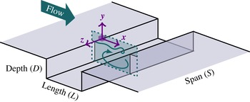
A separated flow over an open cavity (figure 1) is primarily characterised by the enhancement of self-sustained oscillations. As the incoming flow passes successively backward- and forward-facing steps – making a rectangular cavity – Kelvin–Helmholtz travelling waves arise in the shear layer and lock on the cavity length
 $L$
due to an acoustic feedback loop between impingement and separation (Powell Reference Powell1953, Reference Powell1995). These locked-on waves translate into self-sustained oscillations of the shear layer. Spectrally, they correspond to a series of well-defined peaks, whose non-harmonic distribution has been empirically modelled in the compressible regime by Rossiter (Reference Rossiter1964). When the flow is incompressible, the acoustic feedback can be considered as instantaneous. The locked-on frequencies
 $f_{n}$
thus approximately satisfy the simple expression
 $$\begin{eqnarray}f_{n}L/U_{0}\approx n/2,\end{eqnarray}$$
where
 $U_{0}$
is the external velocity and
 $n\in \mathbb{N}^{\ast }$
is the number of cycles between separation and reattachment. Consider a laminar incoming flow, for which
 ${\it\theta}_{0}$
is the momentum thickness of the boundary layer at separation. The dimensionless cavity length
 $L/{\it\theta}_{0}$
is the primary control parameter of the self-sustaining phenomenon (Powell Reference Powell1961; Sarohia Reference Sarohia1977; Rockwell & Naudascher Reference Rockwell and Naudascher1978; Yamouni, Sipp & Jacquin Reference Yamouni, Sipp and Jacquin2013).
Sketch of the geometry under study. Flow features are illustrated in the (
 $x,y$
)-plane (normal to the bottom of the cavity).

1.1. Motivation
Self-sustained oscillations and vortex–edge interactions are responsible for noise generation and drag. They can also lead to structural damage. As such, impinging shear layer waves and associated amplitude modulations (AMs) have been of primary interest in the literature, notably in the extensive work of Rockwell and coworkers (Rockwell Reference Rockwell1977; Knisely & Rockwell Reference Knisely and Rockwell1982; Ziada & Rockwell Reference Ziada and Rockwell1982). On the other hand, very low modulating frequencies – more than 10 times lower than locked-on frequencies – are generally disregarded. AMs at such very low frequencies have still been unambiguously identified in several studies (Neary & Stephanoff Reference Neary and Stephanoff1987; Kegerise et al.
Reference Kegerise, Spina, Garg and Cattafesta III2004; Delprat Reference Delprat2006; Malone et al.
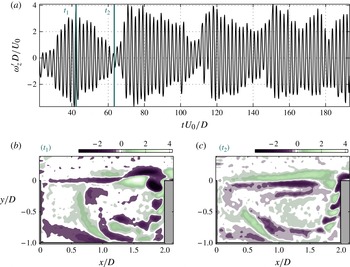
Reference Malone, Debiasi, Little and Samimy2009; Delprat Reference Delprat2010; Vikramaditya & Kurian Reference Vikramaditya and Kurian2012). An illustration of such a phenomenon is given in figure 2. In terms of signal processing, the shear layer locked-on mode constitutes a carrier wave with an envelope evolving over much larger time scales. In dimensionless time based on external velocity and cavity depth,
 $t\,U_{0}/D$
, the period of the carrier wave is 2 while the period of the envelope is around 40; that is, 20 times larger. The snapshots of the vorticity fluctuations in figure 2(b,c) show the spatial dynamics of the flow corresponding respectively to high- and low-amplitude oscillations in the time series. Intense vortices impinging onto the cavity edge are observed when the envelope is maximal, while shear layer waves are drastically damped when the envelope is close to zero.
Vorticity fluctuations
 ${\it\omega}_{z}^{\prime }D/U_{0}$
of time-resolved particle image velocimetry (TRPIV) data in an (
 $x,y$
)-plane, for
 $L/D=2.0$
and
 $L/{\it\theta}_{0}=82$
(
 $U_{0}=1.38\ \text{m}\ \text{s}^{-1}$
). (a) Time series extracted at
 $(x,y)=(1.5\,D,0)$
. (b,c) Two snapshots characteristic of high-amplitude and low-amplitude oscillations, respectively.

This work demonstrates that similar AMs by very low frequencies occur consistently in different experiments and for a wide range of control parameters. An understanding of such a consistent pattern related to severe flow variations could turn out to be crucial for the quantification and control of the shear layer locked-on waves. To this end, the present work identifies the source of the lowest frequencies in open cavity flows, as well as their effects on the self-sustained oscillations of the impinging shear layer.
1.2. Three-dimensional dynamics in cavity flows
In studies dealing with self-sustained oscillations of the shear layer, open cavity flows are often considered as two-dimensional to a first approximation. The spanwise extension of the flow may still have non-negligible influence on the secondary features. This was notably developed by Larchevêque, Sagaut & Labbé (Reference Larchevêque, Sagaut and Labbé2007), who addressed the occurrence of symmetry breakings, associated with spanwise fluctuations of the inner flow. In Neary & Stephanoff (Reference Neary and Stephanoff1987) and more recently in Delprat (Reference Delprat2010), the three-dimensional organisation of the flow was also pointed out to interpret AMs of shear layer waves by very low frequencies.
The first three-dimensional effects are concerned with the influence of the spanwise boundary conditions. In strict terms, spanwise-invariant basic states require that endwalls be non-existent; that is, either periodical spanwise boundary conditions or infinite span (
 $S\rightarrow \infty$
). However, in practice, the presence of endwalls is prevalent, which makes the basic state three-dimensional. The influence of the endwalls depends on the cavity span/depth ratio
 $S/D$
. We state that cavity geometries can be split into two classes.
-
(i) Cavities where
 $S\sim D$
constitute fully three-dimensional geometries with no salient direction in the flow. Such systems are not treated here but have notably been investigated in Larchevêque et al. (Reference Larchevêque, Sagaut, Lê and Comte2004) and Woo, Kim & Lee (Reference Woo, Kim and Lee2007).
-
(ii) Cavities with larger spanwise extensions – basically where
$S/D>4$
– involve almost two-dimensional flows; that is, mainly streamwise–crosswise dynamics. Nevertheless, no-slip spanwise boundary conditions do have secondary effects. According to observations of Koseff & Street (Reference Koseff and Street1984b
), Guermond et al. (Reference Guermond, Migeon, Pineau and Quartapelle2002) and Migeon, Pineau & Texier (Reference Migeon, Pineau and Texier2003) in lid-driven cavities, a steady centripetal flow forms at the endwalls. Similarly to what is observed in Bödewadt layers (Bödewadt Reference Bödewadt1940; Fernandez-Feria Reference Fernandez-Feria2000), the outer flow of the main recirculation is drawn towards the endwalls while a counter-flow is reinjected along the centreline. In Albensoeder, Kuhlmann & Rath (Reference Albensoeder, Kuhlmann and Rath2001), endwalls result in buffer regions encompassing about a quarter of the span. In open cavities, the suction induced by endwall layers is also reported by Faure et al. (Reference Faure, Adrianos, Lusseyran and Pastur2007, Reference Faure, Pastur, Lusseyran, Fraigneau and Bisch2009), but the buffer regions are much smaller.


From now on, we only consider cavities with large spanwise extension. These primarily two-dimensional flows are subject to basically two types of three-dimensional instabilities: secondary instabilities in the impinging shear layer and centrifugal instabilities within the recirculating flow.
The first type of three-dimensional (3D) instability is intrinsic to the shear layer developing over the cavity. Shear flows are known to bifurcate from 2D vortex shedding towards three-dimensionally organised dynamics through secondary instabilities (Taylor Reference Taylor1923). In particular, the three-dimensional nature of impinging flows was first reported by Görtler (Reference Görtler1955). Following the work of Benney & Lin (Reference Benney and Lin1960), Miksad (Reference Miksad1972) demonstrated that 3D dynamics can be produced by nonlinear wave interactions in free shear layers. Rockwell and coworkers applied the same approach to shear layers impinging onto an edge, notably in Rockwell & Naudascher (Reference Rockwell and Naudascher1979). Very low frequencies were not specifically mentioned, but the perturbation of the locked-on waves by three-dimensional dynamics was incontestable. In Rockwell & Knisely (Reference Rockwell and Knisely1980), shear layer travelling waves underwent important spanwise distortions in the form of streamwise vortices. Streamwise vorticity was described as ‘three-dimensionalities enhanced and mitigated in the impingement region’. The ‘upstream convection of non-uniformities’ was only mentioned as a secondary effect. Although experimental techniques could not give access to the precise characteristics of 3D dynamics at the time, spanwise wavelengths were approximated to the order or half the order of the streamwise wavelength.
Since then, the secondary instability of free shear layers has continued to be the subject of numerous experimental studies, among which are the works by Jimenez (Reference Jimenez1983) and Lasheras & Choi (Reference Lasheras and Choi1988). The physical mechanism at play was described as the strain induced between two shed vortices giving rise to streamwise vortex tubes. The spanwise length scale associated with these streamwise vortex tubes largely depends on the initial conditions. The sensibility to the initial conditions at separation was notably demonstrated by Lasheras & Choi (Reference Lasheras and Choi1988). They made use of corrugated plates to initialise the free shear layers with sinusoidal perturbation of various spanwise wavelengths. These conclusions were supported by the numerical investigation of Metcalfe et al. (Reference Metcalfe, Orszag, Brachet, Menon and Riley1987), who showed that plane shear layers are unstable with regards to 3D perturbations for a wide range of spanwise wavenumbers.
Another three-dimensional instability is at play in cavity flows regardless of the shear layer vortex shedding. The recirculating flow inside the cavity can undergo centrifugal instabilities. For the past three decades, the bifurcation of initially two-dimensional recirculating flows towards three-dimensional states has indeed received noticeable attention.
Over the years, linear stability analyses have consistently shown that recirculating flows become globally unstable with regards to spanwise-periodic disturbances for relatively low Reynolds numbers. The recirculating flow bifurcates from a steady (two-dimensional) basic state towards a three-dimensionally structured flow. The onset of such 3D disturbances is attributed to centrifugal instabilities (Sipp & Jacquin Reference Sipp and Jacquin2000). This was notably observed in the case of a recirculation induced by a backward-facing step; see, for instance, Barkley, Gomes & Henderson (Reference Barkley, Gomes and Henderson2002) and Beaudoin et al. (Reference Beaudoin, Cadot, Aider and Wesfreid2004). Cavity flows belong to the same class of recirculating flows. Lid-driven cavities are subject to the rise of spanwise waves along the steady recirculation (Ramanan & Homsy Reference Ramanan and Homsy1994; Albensoeder et al.
Reference Albensoeder, Kuhlmann and Rath2001; Theofilis Reference Theofilis2003; Gonzalez et al.
Reference Gonzalez, Ahmed, Kühnen, Kuhlmann and Theofilis2011) as well as open cavities (Brès & Colonius Reference Brès and Colonius2008; Meseguer-Garrido et al.
Reference Meseguer-Garrido, de Vicente, Valero and Theofilis2011; de Vicente et al.
Reference de Vicente, Basley, Meseguer-Garrido, Soria and Theofilis2014; Meseguer-Garrido et al.
Reference Meseguer-Garrido, de Vicente, Valero and Theofilis2014). Global stability analyses have shown that marginal stability curves actually depend on multiple control parameters, all based on the cavity depth
 $D$
, from the Reynolds number
 $\mathit{Re}_{D}$
to the dimensionless boundary layer thickness
 ${\it\theta}_{0}/D$
and the cavity shape ratio
 $L/D$
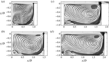
. The underlying control parameter is in fact the Rayleigh discriminant along the recirculating flow inside the cavity. Indeed, Rayleigh discriminant distributions demonstrate that basic states are centrifugally unstable within the shear regions between the curved streamlines of the recirculation and the cavity walls. This is evidenced notably in Brès & Colonius (Reference Brès and Colonius2008) for open cavity flows. Based on experimental mean flows, figure 3 reproduces similar results but shows at the impingement another strongly centrifugally unstable region, probably due to higher control parameters. One should note also the spiral-like streamlines that entail an out-of-plane flow within the main recirculation. Unstable eigenmodes resulting from centrifugal instabilities organise as spanwise waves, either steady or travelling. The growing disturbances wind around the main recirculation and scale on the cavity depth
 $D$
. The corresponding wavenumbers
 ${\it\beta}$
are typically such that
 $$\begin{eqnarray}4\lesssim {\it\beta}=\frac{2{\rm\pi}D}{{\it\lambda}_{z}}\lesssim 15,\end{eqnarray}$$
where
 ${\it\lambda}_{z}$
is the spanwise wavelength (Albensoeder et al.
Reference Albensoeder, Kuhlmann and Rath2001; Brès & Colonius Reference Brès and Colonius2008; Meseguer-Garrido et al.
Reference Meseguer-Garrido, de Vicente, Valero and Theofilis2011; Basley Reference Basley2012; de Vicente et al.
Reference de Vicente, Basley, Meseguer-Garrido, Soria and Theofilis2014; Meseguer-Garrido et al.
Reference Meseguer-Garrido, de Vicente, Valero and Theofilis2014). It is important to note that all unstable travelling eigenmodes reported in the literature are associated with particularly low frequencies – see Chiang, Sheu & Hwang (Reference Chiang, Sheu and Hwang1998), Theofilis (Reference Theofilis2003), Theofilis, Duck & Owen (Reference Theofilis, Duck and Owen2004), Brès & Colonius (Reference Brès and Colonius2008) and references therein. Very recently, the extensive parametric study presented by Meseguer-Garrido et al. (Reference Meseguer-Garrido, de Vicente, Valero and Theofilis2014) has identified the unstable and least stable branches of oscillating eigenmodes for a wide range of parameters. In brief, the frequencies
 $f_{ci}$
entailed by centrifugal instabilities are comprised in the range of Strouhal numbers based on cavity depth
 $$\begin{eqnarray}\mathit{St}_{ci}=f_{ci}D/U_{0}\lesssim 0.05.\end{eqnarray}$$
Streamlines and distribution of the Rayleigh discriminant
 ${\it\eta}$
calculated using the mean flow computed from PIV data in a plane normal to the bottom of the cavity (see § 2.1 for details). Shaded areas correspond to
 ${\it\eta}>0$
. (a)
 $L/D=1.0$
,
 $L/{\it\theta}_{0}=54$
; (b)
 $L/D=1.5$
,
 $L/{\it\theta}_{0}=70$
; (c)
 $L/D=1.75$
,
 $L/{\it\theta}_{0}=96$
; (d)
 $L/D=2.0$
,
 $L/{\it\theta}_{0}=96$
. See the similar study in Brès & Colonius (Reference Brès and Colonius2008) for details and comparison.

In the saturated regime, the spanwise waves embodied by the eigenmodes develop into alleys of counter-rotating vortex pairs coiled around the recirculating flow. Numerous studies on both lid-driven and shear-driven cavities have reported the appearance of such salient spiral eddies – often referred to as Taylor–Görtler-type vortices – spanwise-distributed within the inner flow. Lid-driven cavities have often been preferred as they offer controlled and simple boundary conditions, avoiding any external influence. Various geometries have been investigated, from one-sided lid-driven rectangular cavities (Koseff & Street Reference Koseff and Street1984a
,Reference Koseff and Street
b
,Reference Koseff and Street
c
; Aidun, Triantafillopoulos & Benson Reference Aidun, Triantafillopoulos and Benson1991; Chiang et al.
Reference Chiang, Sheu and Hwang1998; Albensoeder et al.
Reference Albensoeder, Kuhlmann and Rath2001; Migeon et al.
Reference Migeon, Pineau and Texier2003; Theofilis et al.
Reference Theofilis, Duck and Owen2004; Albensoeder & Kuhlmann Reference Albensoeder and Kuhlmann2006) to two-sided driven cavities (Kuhlmann, Wanschura & Rath Reference Kuhlmann, Wanschura and Rath1997; de Vicente Reference de Vicente2010), from triangular cavities (Gonzalez et al.
Reference Gonzalez, Ahmed, Kühnen, Kuhlmann and Theofilis2011) to periodically driven cavities (Blackburn & Lopez Reference Blackburn and Lopez2003; Vogel, Hirsa & Lopez Reference Vogel, Hirsa and Lopez2003). In every case, spanwise-periodic dynamics spontaneously arise and organise as Taylor–Görtler-type vortices whose wavelengths
 ${\it\lambda}_{z}\sim D$
fairly match those of the eigenmodes. Open cavity flows involve more complexity caused by shear layer vortex shedding. However, the inner flow remains mainly steady and still resembles that of a lid-driven cavity for sufficiently low
 $L/{\it\theta}_{0}$
. Recent studies dealing with open cavities have indeed reported spanwise wave alleys of Taylor–Görtler-type vortices, both experimentally (Faure et al.
Reference Faure, Adrianos, Lusseyran and Pastur2007; Douay et al.
Reference Douay, Guéniat, Pastur, Lusseyran and Faure2011; Basley Reference Basley2012; Basley et al.
Reference Basley, Soria, Pastur and Lusseyran2014; de Vicente et al.
Reference de Vicente, Basley, Meseguer-Garrido, Soria and Theofilis2014) and in simulations (Brès & Colonius Reference Brès and Colonius2008; Faure et al.
Reference Faure, Pastur, Lusseyran, Fraigneau and Bisch2009).
When the dimensionless cavity length
 $L/{\it\theta}_{0}$
increases, the shear layer that develops above an open cavity becomes strongly unstable. Self-sustained oscillations induce unsteadiness, mixing with the inner flow. An unsteady base flow entails different stability properties as the fast-scale disturbances from the shear layer might disrupt the growth of slower three-dimensional dynamics. On the other hand, the mixing implied by shear layer flapping motion amplifies the recirculation; hence, it enhances the centrifugal effects inside the cavity. In fact, observations suggest that Taylor–Görtler vortices actually endure in spite of the shear layer disturbances. For instance, the direct numerical simulations by Chang, Constantinescu & Park (Reference Chang, Constantinescu and Park2006), Podvin et al. (Reference Podvin, Fraigneau, Lusseyran and Gougat2006) and Brès & Colonius (Reference Brès and Colonius2008) reveal inner-flow spanwise waves coexisting with Kelvin–Helmholtz vortex shedding. Recently, this coexistence was also observed in an experimental study by the authors (Basley et al.
Reference Basley, Pastur, Delprat and Lusseyran2013) and in Guéniat, Pastur & Lusseyran (Reference Guéniat, Pastur and Lusseyran2014).
If both phenomena can coexist, nonlinear interactions between inner-flow centrifugal instabilities and shear layer waves are likely to occur. To the best of the authors’ knowledge, the link between the spanwise dynamics inside the cavity and AMs of the shear layer oscillations was first observed in Neary & Stephanoff (Reference Neary and Stephanoff1987). There, oscillations at the locked-on frequency were modulated by a frequency about ten times lower. The modulating frequency was interpreted as the result of spanwise time variations of the main recirculation. Later, Pereira & Sousa (Reference Pereira and Sousa1995) also attributed low-frequency modulations to the recirculating flow inside the cavity. In addition, the works of Delprat (Reference Delprat2006, Reference Delprat2010) used a signal processing approach to highlight the impact of AMs on compressible cavity flows. In Delprat (Reference Delprat2006), the Rossiter formula was reinterpreted through modulations by a low frequency. Then, Delprat (Reference Delprat2010) proposed a model based on the combination of two modulation mechanisms to connect Rossiter modes with low frequencies. Interestingly, the lowest modulating frequencies identified in Delprat (Reference Delprat2010) were systematically consistent with time scales typically associated with inner-flow centrifugal instabilities (expression (1.3)). These studies and observations all suggest that some AM process of the shear layer oscillations might be directly induced by Taylor–Görtler vortices inside the cavity.
Should such a connection between inner-flow centrifugal instabilities and shear layer waves exist, the nonlinear coupling may be either (i) local, that is, dependent on the position in the flow, or (ii) global. Scenario (i) relies on local nonlinearities at play between the shear layer vortices – the carrier wave – and the slow-moving 3D vortices filling the inner flow – the low-frequency source. As this source implies both temporal and spanwise fluctuations, the AM is expected to vary along the span. In contrast, hypothesis (ii) involves a global modulation, for which the envelope of the shear layer remains basically spanwise-invariant. In this respect the coupling takes place regardless of the spatial extension of the flow and the AM is temporal only.
1.3. Outline of the study
The previous section has reviewed the three-dimensional instabilities at play in open cavity flows. The 3D effects are generally investigated apart from the self-sustaining mechanism. In contrast, this work focuses on the influence of 3D instabilities on the locked-on waves of the shear layer.
The study is based on two experimental campaigns, which are described in § 2. The 3D organisation of the flow is investigated using time-resolved particle image velocimetry (TRPIV) measurements in two planes.
The discussion of the results encompasses §§ 3–5. We demonstrate that centrifugal instabilities arising in the inner flow are responsible for drastic modulations of the self-sustained oscillations.
In § 3, the lowest frequencies of the flow are identified throughout the parameter space. Nonlinear interactions between these very low frequencies and the shear layer locked-on modes are ascertained and correspond to AMs of the self-sustained oscillations of the shear layer.
In § 4, the spatial dynamics associated with the very low modulating frequencies is identified as slow-moving large-scale structures that coil up inside the cavity. The spanwise extension of the flow is investigated: the inner flow experiences highly coherent spanwise undulations. These three-dimensional waves are characteristic of the centrifugal instabilities along the recirculating flow.
In § 5, the study concentrates on the mechanism of interaction between centrifugal instabilities and shear layer waves. The results show unvaryingly a strong time correlation between the AM of the shear layer and the slow dynamics of the inner flow. The modulation is almost strictly temporal, which indicates a global coupling. The spanwise time correlations suggest that the coupling is related to a beating induced by interference of the spanwise travelling waves.
Our conclusions are presented in § 6.
2. Experiments
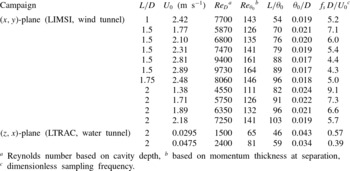
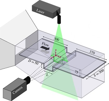
This work is based on experimental results obtained from two TRPIV campaigns, whose parameters are listed in table 1. On the one hand, wind-tunnel experiments (LIMSI) focus on the primary dynamics of the flow, that is the shear layer waves and the recirculating flow inside the cavity. On the other hand, the water-tunnel campaign (LTRAC) is concerned with the spanwise extension of the flow.
Characteristics and control parameters of the TRPIV campaigns.

2.1. High-frame-rate PIV in a normal plane
For the experimental campaign at the LIMSI, high-speed PIV measurements are performed in an (
 $x,y$
)-plane, streamwise and normal to the bottom of the cavity, with a frame rate of 500 Hz (figure 4). The velocity field sampling frequency is 250 Hz. The Shannon criterion is satisfied since all frequencies of the flow are typically below 100 Hz. The cavity depth of
 $D=50\ \text{mm}$
and the span of
 $S=6\,D$
are fixed. By changing both the cavity length
 $L$
and the incoming velocity
 $U_{0}$
, a wide range of the parameter space is encompassed (table 1). The experimental set-up and datasets are described in detail in Basley et al. (Reference Basley, Pastur, Lusseyran, Faure and Delprat2011), Basley (Reference Basley2012) and Basley et al. (Reference Basley, Pastur, Delprat and Lusseyran2013).
Sketch of the experimental set-up used for high-frame-rate PIV measurements in the wind tunnel at LIMSI. The frame of reference is centred in the leading edge at half-span. The cavity length can be varied so that
 $L/D=\{1.0;1.5;1.75;2.0\}$
. TRPIV is performed in an (
 $x,y$
)-plane (normal to the bottom of the cavity) at
 $z=-0.4\,D$
.

2.2. High-resolution PIV in a spanwise plane
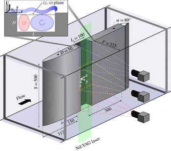
The experiments conducted at the LTRAC aim at identifying the spanwise dynamics of the flow. Details can be found in Basley (Reference Basley2012) and de Vicente et al. (Reference de Vicente, Basley, Meseguer-Garrido, Soria and Theofilis2014). The results consist of high-resolution PIV data of a (
 $z,x$
)-plane, parallel to the bottom of the cavity at
 $y/D=-0.1$
(figure 5). The cavity depth
 $D=50\ \text{mm}$
is unchanged and
 $L/D$
is set to 2. The cavity span,
 $S=10\,D$
, is larger than that of the LIMSI experiments, so as to better identify spanwise wavelengths. However, it is worth remarking that in both cases the spanwise extension is large enough to ensure that the mean flow is primarily two-dimensional, with the influence of the endwalls remaining secondary to the intrinsic stability properties of the recirculating inner flow. Particle images are recorded by three synchronised
 $4904\times 3280\ \text{px}$
cameras, then are processed by an advanced cross-correlation algorithm (Soria Reference Soria1996, Reference Soria1998; Soria, Cater & Kostas Reference Soria, Cater and Kostas1999). The resulting velocity fields (
 $164\times 823$
vectors) are obtained through data merging.
The experimental set-up used for high-resolution PIV measurements in the water tunnel at LTRAC. Time-resolved PIV is performed in a (
 $z,x$
)-plane (spanwise) at
 $y=-0.1\,D$
.

The two investigated cases
 $\mathit{Re}_{D}=\{1500;2400\}$
correspond to low incoming velocities
 $U_{0}$
in water, as reported in table 1. As a result, the two dimensionless sampling frequencies
 $f_{s}\,D/U_{0}=\{0.57,0.39\}$
fully satisfy the Shannon criterion with regards to spanwise dynamics of the inner flow (expression (1.3)) in spite of the low repetition rate – the time interval between velocity fields is typically 3 s. Regarding the shear layer oscillations, control parameters such that
 $L/{\it\theta}_{0}\leqslant 60$
imply that the first locked-on mode (
 $n=1$
) is selected (Sarohia Reference Sarohia1977; Basley et al.
Reference Basley, Pastur, Delprat and Lusseyran2013). In other words, the shear layer experiences only one cycle of oscillation within the cavity length
 $L$
, corresponding to the wavelength
 ${\it\lambda}_{n=1}\sim L$
. The associated frequencies are thus
 $f_{n=1}\,L/U_{0}\sim 0.5$
– see (1.1) – and the corresponding Strouhal number based on
 $D$
is
 $f_{n=1}\,D/U_{0}\sim 0.25$
. As reported in table 1, the first case (
 $\mathit{Re}_{D}=1500$
,
 $L/{\it\theta}_{0}=46$
) is sampled at
 $f_{s}\,D/U_{0}=0.57$
, making the shear layer oscillations time-resolved. On the other hand, the second investigated case (
 $\mathit{Re}_{D}=2400$
,
 $L/{\it\theta}_{0}=59$
) is sampled at
 $f_{s}\,D/U_{0}=0.39$
. This results in aliasing the shear layer oscillations at the apparent frequency
 $(\,f_{s}-f_{n=1})\,D/U_{0}\sim 0.39-0.25\sim 0.14$
. It should be noted, however, that such an aliasing has limited damage since it does not overlap with other frequencies of the flow.
3. Spectral signature and AM
This section focuses on characterising the slowest dynamics of the flow, in relation to the severe modulations of the shear layer waves. The very low frequencies are identified in power spectra of velocity fluctuations. Their nonlinear interactions with the shear layer oscillations are then revealed using bicoherence.
3.1. The lowest frequencies of the flow
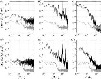
Although shear layer vortex shedding constitutes the most salient phenomenon of open cavity flows, high energy is also typically observed for low frequencies in the spectrum. This signature is notably exhibited by time series of velocity fluctuations, as illustrated by figure 6. The power spectra are obtained using the window-averaging method (Welch Reference Welch1967) out of TRPIV data from the LIMSI campaign. One recognises narrow-banded peaks associated with the self-sustained oscillations of the shear layer in figure 6(b,e). However, another range of much lower frequency spikes becomes apparent as the only salient feature of the spectrum inside the cavity (figure 6 c, f). Indeed, the lowest frequencies of the spectrum have often been disregarded as they can correspond to fluctuations of the upstream flow inherent to experimental facilities. In order to rule out any effect due to forcing of disturbances in the incoming flow, figure 6 compares normalised spectra of an open cavity flow (black curves) with the spectrum in the absence of the cavity (gray curve). The results demonstrate that the free stream exhibits energy levels far lower than those of the cavity flow: about three orders of magnitude with respect to the noticeable peaks of the spectrum, both within the shear layer and inside the cavity. One also notes that there is no correspondence between the highest energy levels of the free stream and any of the peaks observed in the spectra of the flow. The low frequencies spiking in the spectra of figure 6 can only be attributed to the intrinsic dynamics of the open cavity flow.
Comparative plots of power spectra in the wind tunnel at LIMSI, with
 ${\it\delta}f$
the frequency step. Streamwise velocity fluctuations are extracted from
 $(x,y)$
-planar TRPIV datasets at three different locations (black), to be compared with the free stream (gray); that is, when the cavity is removed. Two cases are presented: (a–c)
 $L/D=2.0$
,
 $U_{0}=1.71\ \text{m}\ \text{s}^{-1}$
,
 $L/{\it\theta}_{0}=91$
and (d–f)
 $L/D=1.5$
,
 $U_{0}=2.32\ \text{m}\ \text{s}^{-1}$
,
 $L/{\it\theta}_{0}=79$
. (a) Incoming flow (
 $x=0;y=0.4\,D$
). (b) Shear layer (
 $x=1.7\,D;y=0$
). (c) Inner flow (
 $x=0.6\,D;y=-0.8\,D$
). (d) Incoming flow (
 $x=0;y=0.4\,D$
). (e) Shear layer (
 $x=1.4\,D$
;
 $y=0$
). ( f) Inner flow (
 $x=1.1\,D$
;
 $y=-0.9\,D$
).

Such a highly energetic low-frequency range is in fact commonly encountered for all investigated cases. To support this assertion, streamwise laser Doppler velocimetry (LDV) measurements were performed for various control parameters. Time series were acquired near the impingement over 3 min, i.e.
 ${\sim}4000$
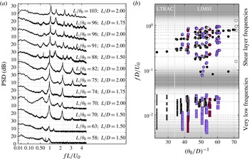
shear layer cycles. Details are given in Basley et al. (Reference Basley, Pastur, Lusseyran, Faure and Delprat2011, Reference Basley, Pastur, Delprat and Lusseyran2013). The resulting power spectral densities are plotted in figure 7(a). On top of the narrow-peaked frequencies of the shear layer, scaling on
 $L$
, the spectra consistently exhibit a broad-band component at very low frequencies. As mentioned in the introduction, the occurrence of very-low-frequency peaks has been reported in earlier works, but the nature of the underlying physics remains unclear.
Spectral signature of the flow throughout the parameter space. (a) Power spectral densities are computed out of streamwise LDV measurements
 $u^{\prime }(t)$
in the impinging shear layer, at
 $(x_{ldv},y_{ldv})\simeq (0.95\,L,0.1\,D)$
. For the sake of clarity, each curve is incremented by 30 dB. It should be noted that the curve thickness represents the 95 % confidence interval. (b) Dominant frequencies of the flow are extracted out of both LDV and TRPIV data from both LIMSI and LTRAC campaigns (see the text for more details):
 $D$
-based Strouhal numbers corresponding to most energetic local maxima are plotted against
 $({\it\theta}_{0}/D)^{-1}$
for, from light to dark symbols,
 $L/D=1$
,
 $L/D=1.5$
,
 $L/D=1.75$
,
 $L/D=2$
.

3.2. Two scales in the spectrum
In order to identify the source of these broad-banded low frequencies and their interactions with the shear layer, space-extended data are required to observe the associated dynamics wherever it is the most energetic. That is the reason why figure 7(b) uses TRPIV data to complete the LDV measurements. The use of TRPIV time series allows us to extract time spectra throughout the flow. The spectrum can hence be integrated in space to determine unambiguously the most significant frequencies. This is particularly useful when dealing with broad-banded signatures such as the very low frequencies discussed herein. The results of this analysis are presented in figure 7(b), which reports the salient frequencies of the flow within the parameter space. It should be noted that the shear layer frequency
 $f\,DU_{0}=0.245$
reported for
 $({\it\theta}_{0}/D)^{-1}=29.6$
(LTRAC campaign) has been dealiased, as explained in the previous section. The diagram reveals that the spectral signature consistently splits into two distinct time scales.
The first scale –
 $f\,D/U_{0}\gtrsim 0.2$
– classically corresponds to fast dynamics dominated by the self-sustained oscillations of the shear layer. These frequencies are primarily associated with locked-on cycles of vortex shedding. The shear layer dynamics also often entails edge frequencies: secondary peaks related to AMs at the impingement. Other works by the authors (Pastur et al.
Reference Pastur, Lusseyran, Fraigneau and Podvin2005; Lusseyran, Pastur & Letellier Reference Lusseyran, Pastur and Letellier2008; Basley et al.
Reference Basley, Pastur, Lusseyran, Faure and Delprat2011, Reference Basley, Pastur, Delprat and Lusseyran2013) were devoted to these AMs of the impinging shear layer. For instance, one may remark that several frequencies are sensibly lower than the typical shear layer frequencies, basically around
 $f\,D/U_{0}\sim 0.1$
. These spectral components departing from the rest were specifically treated in Basley et al. (Reference Basley, Pastur, Delprat and Lusseyran2013). The reader may refer to the extensive literature concerning shear layer locked-on waves for greater detail, but the present study aims at far lower modulating frequencies, as introduced in § 1.1.
The second scale represents broad-banded slow dynamics and is far less documented. It consists of scattered frequencies such that
 $0.005\lesssim f\,D/U_{0}\lesssim 0.04$
, for which no simple pattern can be deduced. It should be noted that only the most energetic and statistically pertinent peaks of the low-frequency range are reported. Low-presence-rate components and FFT-induced noise are removed using window-averaging (Welch Reference Welch1967) and confidence intervals are estimated by
 ${\it\chi}$
-functions. If no clear local maximum can be found (even in the inner flow), no frequency is reported. Unlike shear layer waves, the very low frequencies do not scale on
 $L$
since no separation appears between different
 $L/D$
ratios. On the other hand, frequencies such that
 $f\,D/U_{0}\sim 0.02$
are consistent with centrifugal instabilities (expression (1.3)). In the following, Strouhal numbers are always based on the cavity depth
 $D$
.
3.3. Modulating frequencies in the inner flow
The separation of the dynamics into the two aforementioned scales can also be illustrated by the spatial evolution of the spectrum throughout the (
 $x,y$
)-plane, using the two-component two-dimensional velocity field
 $$\begin{eqnarray}\boldsymbol{U}(\boldsymbol{x},t)=[\overline{u}(\boldsymbol{x})+u^{\prime }(\boldsymbol{x},t)]\boldsymbol{e}_{x}+[\overline{v}(\boldsymbol{x})+v^{\prime }(\boldsymbol{x},t)]\boldsymbol{e}_{y},\end{eqnarray}$$
where
 $\{\overline{u},\overline{v}\}$
are the streamwise and crosswise mean velocities and
 $\{u^{\prime }(t),v^{\prime }(t)\}$
are the streamwise and crosswise velocity fluctuations, at the point
 $\boldsymbol{x}=(x,y)$
. Velocity time series can hereby be extracted from any location in the flow. Figure 8 presents two time series extracted at the impingement and near the bottom of the cavity, respectively, for parameters
 $L/{\it\theta}_{0}=82$
,
 $L/D=2$
,
 $\mathit{Re}_{D}=4550$
.
Velocity fluctuations extracted from TRPIV datasets for
 $L/D=2.0$
,
 $L/{\it\theta}_{0}=82$
(LIMSI campaign); gray,
 $v^{\prime }(1.70\,D,0,t)/U_{0}$
; black,
 $u^{\prime }(D,-0.75\,D,t)/U_{0}$
. (a) Time series are plotted along with (b) the associated power spectra (window averaged). (c) A sketch of the extraction points in the (
 $x,y$
)-plane.

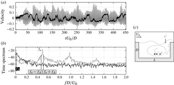
The velocity fluctuations measured at the bottom of the cavity (black curves) are basically free of shear layer waves. The spectral signature is restricted to the low-frequency range, with a broad-banded peak more than 30 dB higher than the rest of the spectrum. More specifically, the spectrum reaches its maximum at a frequency denoted
 $f_{{\it\Delta}}$
, such that
 $\mathit{St}_{{\it\Delta}}=f_{{\it\Delta}}\,D/U_{0}=0.024$
. This signature suggests that the source of low frequencies lies within the inner flow rather than in the shear layer.
In contrast, the crosswise velocity fluctuations near the impingement (grey curves) predominantly reflect the self-sustained oscillations of the shear layer. The associated power spectrum indeed shows the locked-on frequency
 $f_{a}$
, such that
 $\mathit{St}_{a}=f_{a}\,D/U_{0}=0.49$
, and its harmonics
 $2\,f_{a}$
,
 $3\,f_{a}$
. However, we assert that the low frequencies are indirectly present through the sideband peaks denoted
 $f_{a}\pm f_{{\it\Delta}}$
. The appearance of combination frequencies
 $f_{a}\pm f_{{\it\Delta}}$
is the signature of the AM of a carrier wave at the frequency
 $f_{a}$
by a modulating signal, entailing the frequency
 $f_{{\it\Delta}}$
. In terms of flow dynamics, linear combinations of frequencies in the Fourier space correspond to nonlinear interactions in the physical space: the frequencies
 $f_{a}\pm f_{{\it\Delta}}$
indicate quadratic nonlinearities coupling the dynamics associated with
 $f_{a}$
(shear layer oscillations) to a second phenomenon associated with the broad-banded peak around
 $f_{{\it\Delta}}$
.
The third-order spectrum, also known as the bispectrum, enables independent spectral components to be distinguished from nonlinearly coupled modes (Kim et al.
Reference Kim, Beall, Powers and Miksad1980). This tool has been applied to the study of open cavity flows on many occasions, from Knisely & Rockwell (Reference Knisely and Rockwell1982) and Isaacson & Marshall (Reference Isaacson and Marshall1983) to Larchevêque et al. (Reference Larchevêque, Sagaut, Lê and Comte2004) and Gloerfelt (Reference Gloerfelt2006), but only a handful of works have focused the high-order spectral analysis on very low frequencies. Kegerise et al. (Reference Kegerise, Spina, Garg and Cattafesta III2004) and recently Vikramaditya & Kurian (Reference Vikramaditya and Kurian2012) highlighted the occurrence of nonlinear interactions between such low frequencies and the dominant frequencies of the shear layer in the compressible regime. The bispectrum of a temporal signal
 $x(t)$
is the two-dimensional Fourier transform of the third-order cumulant, which is also written as
 $$\begin{eqnarray}B_{xxx}(\,f_{1},f_{2})=\text{E}\left[X(\,f_{1})\,X(\,f_{2})\,X^{\ast }(\,f_{1}+f_{2})\right],\end{eqnarray}$$
where
 $\text{E}[\centerdot ]$
represents the expectation value,
 $X(\,f)$
is the Fourier transform of
 $x(t)$
and
 $\text{}^{\ast }$
denotes the complex conjugate. The bispectrum quantifies the energy exchanges within a triad of waves
 $\{\,f_{1},f_{2},f_{1}+f_{2}\}$
. More precisely, a non-zero value of
 $B_{xxx}(\,f_{1},f_{2})$
implies that
 $f_{1}$
and
 $f_{2}$
waves transfer energy to the third frequency
 $f_{1}+f_{2}$
through quadratic nonlinearities. The bispectrum is often normalised by the power spectrum
 $P_{xx}(\,f)$
to obtain the bicoherence:
 $$\begin{eqnarray}b_{xxx}^{2}(\,f_{1},f_{2})={\displaystyle \frac{|B_{xxx}(\,f_{1},f_{2})|^{2}}{P_{xx}(\,f_{1})\,P_{xx}(\,f_{2})\,P_{xx}(\,f_{1}+f_{2})}}.\end{eqnarray}$$
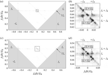
Fourier transform symmetry and the commutativity of expressions (3.2) and (3.3) imply redundancies so that the bispectrum can be fully represented with a triangular domain. The bicoherence diagrams presented in figure 9 confirm the existence of the nonlinearities hypothesised earlier. For different control parameters, the dominant locked-on frequency, denoted
 $f_{a}$
, interacts nonlinearly with the very low frequencies, around
 $f_{{\it\Delta}}$
. As expected, one also observes that the nonlinear saturation of the wave at
 $f_{a}$
conveys energy towards the harmonic
 $2f_{a}$
through the coupling
 $\{\,f_{a},f_{a}\}$
. The characteristics of the coupling mechanism between shear layer waves and slow dynamics of the inner flow are addressed further in § 5. Prior to that, the study focuses on identifying the spatial dynamics associated with the broad-band low frequencies.
Bicoherence computed out of time series of vorticity fluctuations for two cases (LIMSI): (a,b)
 $L/{\it\theta}_{0}=79$
,
 $L/D=1.5$
and (c,d)
 $L/{\it\theta}_{0}=82$
,
 $L/D=2$
. The bispectrum is integrated over space near the impingement along the cavity wall (
 $L-0.15\,D\leqslant x\leqslant L,-0.25\,D\leqslant y\leqslant -0.05\,D$
). Panels (b,d) show close-ups of the nonlinearities between the two frequencies
 $f_{a}$
and
 $f_{{\it\Delta}}$
.

4. Space–time dynamics of the three-dimensional flow
This section makes extensive use of modal decompositions in both space and time to associate each feature of the spectral signature with its underlying spatial structures. The analysis is first conducted in the plane (
 $x,y$
) to deal with the dominant dynamics of the flow (§ 4.1). The spanwise extension of the flow is then investigated using the plane (
 $z,x$
) so as to characterise the three-dimensional waves resulting from centrifugal instabilities (§ 4.2).
4.1. Space–time decomposition in an (
$x,y$
)-plane

The spatial structures associated with the two aforementioned scales – shear layer modes and very low frequencies – are investigated through proper orthogonal decomposition (POD), which is commonly used to extract the most coherent structures of the flow. The detail and generalities about the methodology are not the subject here, but the reader may find helpful information, for instance, in Holmes, Lumley & Berkooz (Reference Holmes, Lumley and Berkooz1996) and Cordier & Bergmann (Reference Cordier and Bergmann2003). For examples of POD applications and developments in fluid mechanics, one may notably refer to the recent works of Iungo & Lombardi (Reference Iungo and Lombardi2011), Kitsios et al. (Reference Kitsios, Cordier, Bonnet, Ooi and Soria2011), Buchmann, Atkinson & Soria (Reference Buchmann, Atkinson and Soria2013), Cammilleri et al. (Reference Cammilleri, Gueniat, Carlier, Pastur, Memin, Lusseyran and Artana2013) and Guéniat et al. (Reference Guéniat, Pastur and Lusseyran2014). In the present case, the decomposition is applied to the vorticity fields
 $$\begin{eqnarray}{\it\omega}_{z}(\boldsymbol{x},t)=\overline{{\it\omega}_{z}}(\boldsymbol{x})+{\it\omega}_{z}^{\prime }(\boldsymbol{x},t),\end{eqnarray}$$
issued from the same (
 $x,y$
)-plane TRPIV measurements as in the previous section (§ 3.3). Proper orthogonal decomposition is performed on vorticity fluctuations
 ${\it\omega}_{z}^{\prime }(\boldsymbol{x},t)$
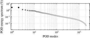
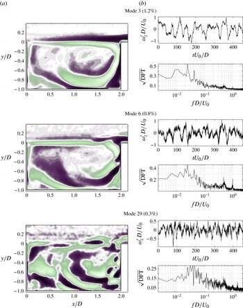
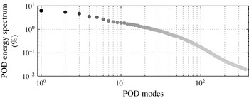
. In brief, the dataset is contained in a single matrix such that snapshots are successively stacked along rows while columns correspond to time series at every point of the field. By applying singular value decomposition to such a matrix, one splits up space and time dynamics into orthogonal modes associating spatial structures with time series. The decomposition leads to the eigenvalues plotted in figure 10. After the first two equally energetic modes, eigenvalues are significantly lower and decrease smoothly. Several examples among the most salient modes are displayed in figures 11 and 12 for shear layer and inner-flow dynamics, respectively.
Proper orthogonal decomposition eigenvalues, out of TRPIV data for
 $L/D=2.0$
,
 $L/{\it\theta}_{0}=82$
in an (
 $x,y$
)-plane; 2048 modes are computed using vorticity fluctuations
 ${\it\omega}_{z}^{\prime }\,D/U_{0}$
.

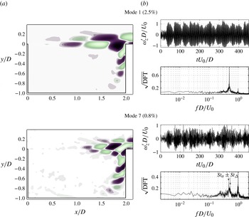
Proper orthogonal decomposition modes representing shear layer dynamics, out of TRPIV data for
 $L/D=2.0$
,
 $L/{\it\theta}_{0}=82$
in an (
 $x,y$
)-plane. Spatial modes (a) are associated with temporal modes (b) plotted as both time series and amplitude spectra.

POD modes representing inner flow slow dynamics, out of TRPIV data for
 $L/D=2.0$
,
 $L/{\it\theta}_{0}=82$
in an (
 $x,y$
)-plane. Spatial modes (a) are associated with temporal modes (b) plotted as both time series and amplitude spectra.

The first two (most energetic) modes represent the dominant shear layer wave, see figure 11 (top). The spatial structure of mode 1 exhibits a locked-on mode consisting of two cycles of vortices shed along
 $L$
. Temporally, mode 1 is restricted to the single narrow-peaked frequency at
 $\mathit{St}_{a}=0.49$
. Mode 2 is in quadrature of phase to mode 1, which denotes a travelling wave. Shear layer dynamics then reappears in mode 7, see figure 11 (bottom). Along with mode 8 in quadrature, they convey a fast travelling wave characteristic of the first harmonic to the dominant shear layer wave (mode 1). As such, the streamwise wavelength entailed by mode 7 is half that of mode 1 and the time power spectrum peaks at the frequency
 $\mathit{St}_{a2}=0.98=2\,\mathit{St}_{a}$
. These POD modes are perfectly consistent with other POD studies from the literature on cavity flows (Rowley, Colonius & Murray Reference Rowley, Colonius and Murray2000; Podvin et al.
Reference Podvin, Fraigneau, Lusseyran and Gougat2006; Gloerfelt Reference Gloerfelt2008). One may also notice the similarity with global Fourier modes obtained in Rowley, Colonius & Basu (Reference Rowley, Colonius and Basu2002), Basley et al. (Reference Basley, Pastur, Lusseyran, Faure and Delprat2011) and Basley et al. (Reference Basley, Pastur, Delprat and Lusseyran2013). It is worth highlighting that AM by very low frequencies is recovered in both shear layer waves. One remarks notably the sideband peaks
 $\mathit{St}_{a}\pm \mathit{St}_{{\it\Delta}}$
in the time spectrum of mode 7.
The slow dynamics of the inner flow is first observed in mode 3, see figure 12. The spatial structures depict large-scale fluctuations carried by the main recirculation and the associated temporal features recover the broad-banded low frequencies peaking at
 $\mathit{St}_{{\it\Delta}}=0.024$
with a secondary peak at
 $\mathit{St}=0.041$
. Modes 4 and 5 exhibit similar dynamics. These modes do not represent streamwise travelling eddies but rather organise as layers of alternate shear vorticity wrapped around the main recirculation. This organisation denotes non-negligible out-of-plane fluctuations. Furthermore, one may notice that the signature is particularly intense within the centrifugally unstable regions – earlier revealed in figure 3 – suggesting three-dimensional dynamics. The three-dimensionality of this slow dynamics is also demonstrated by its absence in 2D simulations. For instance, the salient POD modes reported in Rowley et al. (Reference Rowley, Colonius and Murray2000), Gloerfelt (Reference Gloerfelt2006) and Gloerfelt (Reference Gloerfelt2008) exclusively reflect shear layer waves. On the other hand, the 3D numerical study conducted in Podvin et al. (Reference Podvin, Fraigneau, Lusseyran and Gougat2006) showed similar slow dynamics, actually connected to spanwise oscillations inside the cavity. The latter modes can be compared with results from global Fourier decomposition to bring further insight. Recently, the experimental investigation in Basley et al. (Reference Basley, Pastur, Delprat and Lusseyran2013) used global Fourier modes to identify the low-frequency dynamics in a flow presenting an unusual multi-modulated signature. The extensive study was focused on a single configuration (
 $L/D=1.5$
,
 $L/{\it\theta}_{0}=76$
). The dynamics associated with a very-low-frequency
 $f_{{\it\Delta}}\,D/U_{0}\simeq 0.02$
was consistent with figure 12 and involved spanwise variations.
The present results as well as previous works point to centrifugal instabilities arising along the main recirculation. Such a spatio-temporal signature would result from three-dimensional waves described notably in Brès & Colonius (Reference Brès and Colonius2008), de Vicente et al. (Reference de Vicente, Basley, Meseguer-Garrido, Soria and Theofilis2014) and Meseguer-Garrido et al. (Reference Meseguer-Garrido, de Vicente, Valero and Theofilis2014). Three-dimensional eddies winding around the main vortex, confined in the outer regions along the walls, would travel spanwise across the (
 $x,y$
)-plane.
The rest of the modes do not strictly represent either inner-flow dynamics or shear layer oscillations. Both temporal and spatial modes involve fast-moving structures related to slower events. For instance, modes 6 and 29 – in figure 12 – mix the energetic broad-banded signature of slow dynamics around the main recirculation with features reminiscent of shear layer oscillations. More specifically, the time spectrum associated with mode 6 highlights the broad-banded low frequencies and the shear layer frequency
 $\mathit{St}_{a2}\simeq 1.0$
. For mode 29, the shear layer dynamics is present through the second harmonic at
 $\mathit{St}_{a3}\simeq 1.5$
. Of particular interest is the recurring presence of the sideband peaks
 $\mathit{St}_{a}\pm \mathit{St}_{{\it\Delta}}$
, denoting the AM by
 $\mathit{St}_{{\it\Delta}}$
. This coherence of the slow dynamics inside the cavity with amplitude-modulated fast dynamics of the shear layer confirms the importance of nonlinear interactions between the two phenomena.
4.2. Space–time decomposition in a (
$z,x$
)-plane

The focus is now on the spanwise extension of the flow to investigate the three-dimensional dynamics at play inside the cavity. The subsequent analysis is based on TRPIV measurements performed in a (
 $z,x$
)-plane spanning the cavity at
 $y=-0.1\,D$
for
 $\mathit{Re}_{D}=2400$
,
 $L/{\it\theta}_{0}=59$
,
 ${\it\theta}_{0}/D=0.034$
,
 $L/D=2$
for the experiments described in § 2.2. Since the recordings are time-resolved, space–time decomposition can be used to identify the spanwise dynamics associated with the characteristic frequencies. In a previous study (de Vicente et al.
Reference de Vicente, Basley, Meseguer-Garrido, Soria and Theofilis2014) the analysis was conducted using global Fourier decomposition of crosswise vorticity fluctuations
 ${\it\omega}_{y}^{\prime }$
. The saturated three-dimensional dynamics was characterised with regards to the onset of centrifugal instabilities along the recirculating inner flow. Sets of spanwise-travelling waves were identified in the experiments and the global Fourier modes exhibited patterns that matched locally the eigenmodes that arose from linear stability analysis. As expected, the identified spanwise-travelling waves involved frequencies consistent with centrifugal instabilities (expression (1.3)).
The present investigation aims to relate the spanwise dynamics of the inner flow to AMs of the shear layer waves. The space–time decomposition is achieved using POD applied to the streamwise velocity fluctuations
 $u^{\prime }(z,x,y=-0.1\,D,t)$
. This plane of study offers an ideal location encompassing the shear layer oscillations as well as the recirculating inner flow.
4.2.1. Proper orthogonal decomposition and the Hilbert–Huang transform
Proper orthogonal decomposition eigenvalues are plotted in figure 13. It should be noted that the energy decreases smoothly and that more than two orders of magnitude separate the first from the last of the 365 computed modes. Once spatial and temporal POD modes are obtained, spectral analysis is undertaken to determine the spanwise wavelengths
 ${\it\lambda}_{z}$
and Strouhal numbers characterising this flow. Application of a space Fourier transform provides statistical (integrated) information since it relies on a scalar product. Local estimation of the wave properties of the POD modes brings further insight into the modulations of the identified coherent structures (Basley Reference Basley2012). In that context, the Hilbert–Huang transforms (HHTs) are computed from the POD modes both spanwise and timewise.
Proper orthogonal decomposition eigenvalues out of TRPIV data for
 $\mathit{Re}_{D}=2400$
,
 $L/D=2.0$
,
 $L/{\it\theta}_{0}=59$
,
 ${\it\theta}_{0}/D=0.034$
, in a (
 $z,x$
)-plane, using streamwise velocity fluctuations
 $u^{\prime }$
from 365 snapshots.

Since its development by Huang (Huang, Long & Shen Reference Huang, Long and Shen1996; Huang et al. Reference Huang, Shen, Long, Wu, Shih, Zheng, Yen, Tung and Liu1998; Huang, Shen & Long Reference Huang, Shen and Long1999), the HHT has been extensively utilised to investigate distorted signals resulting from multi-scale and/or modulated dynamics, in particular, nonlinearly saturated waves which involve a non-constant frequency and where the instantaneous frequency varies over one period of oscillation. In that context, HHT is a powerful tool as it enables the precise identification of the instantaneous frequency. The reader may refer to Basley (Reference Basley2012) for the basics of HHT methodology, and an exhaustive discussion is available in Huang et al. (Reference Huang, Shen, Long, Wu, Shih, Zheng, Yen, Tung and Liu1998). In principle, the HHT uses the empirical mode decomposition (EMD) to extract zero-mean oscillatory functions, on which the classical Hilbert transform is applied. The originality of EMD comes from its model-free a posteriori-defined basis. The decomposition relies entirely and directly on the data, without any pre-requirement for the modes resulting from the process. One only assumes that a signal can be decomposed into a set of zero-mean oscillatory modes, referred to as intrinsic mode functions (IMFs). Such functions are obtained by a sifting process, which consists in subtracting from the signal its running average, defined as the local mean value of the inferior and superior envelopes. By applying the same process recursively, the running average eventually tends to zero, with oscillations ending up properly centred. Once an IMF is extracted, the same sifting process is applied to the remaining signal until the residue becomes a constant or contains one oscillation at the most. In brief, an IMF constitutes an oscillating signal, not necessarily sinusoidal, that may involve various length scales and amplitudes but whose mean is always zero. One can thus appreciate that such an oscillatory function can meet the requirements for a Hilbert transform (Pastur et al. Reference Pastur, Lusseyran, Faure, Fraigneau, Pethieu and Debesse2008). Construction of an analytic signal provides the local amplitude and phase of the IMF under consideration. From the phase gradient, the local frequency is estimated, or the local wavenumber if the signal is a function of space. As a result, each IMF provides a Hilbert–Huang spectrum, a function that associates local frequency with local amplitude. In the following, only the most energetic IMF is considered.
4.2.2. Analysis of the spanwise dynamics
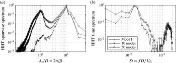
Prior to analysing the POD modes separately, characteristic wavelengths are estimated using the marginal spectrum of the spatial modes altogether. This marginal spectrum is obtained by integrating the Hilbert–Huang spectrum over
 $z$
and summing up the contributions from all spanwise rows. The marginal spectrum is plotted in figure 14(a). The spanwise spectrum highlights two main wavelengths. The first salient wavelength
 ${\it\lambda}_{z}\simeq 10\,D$
represents the cavity span. This corresponds to quasi-two-dimensional dynamics restricted by the endwalls at
 $z=\pm 5\,D$
. This signature is mostly carried by mode I. The rest of the POD modes exhibit wavelengths around
 ${\it\lambda}_{z}=D$
, which is consistent with patterns generated by centrifugal instabilities.
Hilbert–Huang marginal spectra for both spatial (a) and temporal (b) POD modes in a (
 $z,x$
)-plane for
 $\mathit{Re}_{D}=2400$
,
 $L/D=2.0$
,
 $L/{\it\theta}_{0}=59$
,
 ${\it\theta}_{0}/D=0.034$
.

We proceed similarly to identify characteristic frequencies out of the temporal POD modes. The resulting time marginal spectrum is presented in figure 14(b). It involves the two same characteristic scales, one order of magnitude apart, as pointed out in the previous section (§ 3). The dominant Strouhal number at
 $f\,D/U_{0}\sim 0.015$
represents the very low frequencies implied by the inner flow, while the second salient peak observed around
 $f\,D/U_{0}\sim 0.14$
is likely to correspond to aliased frequencies associated with shear layer oscillations. More insight is available through mode-to-mode analysis of the most energetic POD modes. These are illustrated in figures 15–17 along with the corresponding spanwise and timewise Hilbert–Huang spectra.
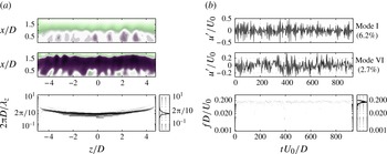
Proper orthogonal decomposition modes
 $\{\text{I,VI}\}$
computed out of TRPIV data for
 $L/D=2.0$
,
 $L/{\it\theta}_{0}=59$
,
 ${\it\theta}_{0}/D=0.034$
, in the (
 $z,x$
)-plane (
 $y=-0.1\,D$
). The spatial modes (a) are associated with the temporal modes (b). Homologous POD modes are brought together and analysed using HHT (bottom) to identify locally the associated wavenumbers and frequencies, along with the marginal (integrated) spectra.

Proper orthogonal decomposition modes
 $\{\text{II,III}\}$
and
 $\{\text{IV,V}\}$
computed out of TRPIV data for
 $L/D=2.0$
,
 $L/{\it\theta}_{0}=59$
,
 ${\it\theta}_{0}/D=0.034$
, in the (
 $z,x$
)-plane (
 $y=-0.1\,D$
). See the caption to figure 15 for more detail.

Modes I and VI recover shear layer vortex shedding, with spatial structures dominated by streamwise-travelling waves spanning the cavity, as seen in figure 15. This pair of modes is characterised by a quasi-constant spanwise wavenumber
 ${\it\beta}=2{\rm\pi}D/{\it\lambda}_{z}\simeq 2{\rm\pi}/10$
(
 ${\it\lambda}_{z}\simeq 10\,D$
), mentioned above with regard to the total marginal HHT spectrum in figure 14. The streamwise wavelength associated with shear layer oscillations can be estimated to be approximately equal to the cavity length, implying one cycle of oscillation (
 $n=1$
) as expected for a dimensionless cavity length of
 $L/{\it\theta}_{0}=59$
. Timewise, such a locked-on mode is associated with a frequency
 $f_{1}\,L/U_{0}\sim 0.5$
(1.1), that is,
 $f_{1}\,D/U_{0}\sim 0.25$
. With a Nyquist frequency at
 $f_{Nyq}=f_{s}/2=0.195\ U_{0}/D$
– see table 1 – such a frequency is aliased at
 $(2\,f_{Nyq}-f_{1})\,D/U_{0}\sim 0.14$
, matching precisely the Strouhal numbers identified by HHT from the POD modes.
Proper orthogonal decomposition modes
 $\{\text{VII,IX,XI}\}$
computed out of TRPIV data for
 $L/D=2.0$
,
 $L/{\it\theta}_{0}=59$
,
 ${\it\theta}_{0}/D=0.034$
, in the (
 $z,x$
)-plane
 $y=-0.1\,D$
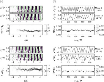
. See the caption to figure 15 for more detail.

The primarily two-dimensional organisation of modes I and VI appears superimposed with spanwise oscillations of lower amplitude. These are more visible in the upstream half of the cavity before being overridden by the growing shear layer oscillations. Furthermore, the temporal signature is once again amplitude modulated by very low frequencies around
 $0.015\,U_{0}/D$
, confirming that this AM occurs consistently for various control parameters.
Modes II, III and IV, V organise as two pairs of homologous patterns in phase quadrature (figure 16). Each pair conveys a highly coherent monochromatic spanwise-travelling wave. The well-defined phase fronts are parallel, yet slightly skewed, as they stand for helical structures coiling up the recirculating flow. Modes II and III represent a left-travelling wave associated with, on average, the wavenumber
 ${\it\beta}\approx 2{\rm\pi}$
and Strouhal number
 $f\,D/U_{0}\approx 0.016$
, while modes III and IV depict a right-travelling wave associated with a similar wavenumber and a slightly lower Strouhal number of
 $f\,D/U_{0}\approx 0.014$
. For both waves, nonlinear distortion is revealed by wavenumber fluctuations along the span. These saturated spanwise waves of wavelengths
 ${\it\lambda}_{z}\sim D$
result from centrifugal instabilities onset along the recirculation inside the cavity.
In fact, these two pairs of POD modes entail the same dynamics as the global Fourier modes in Basley (Reference Basley2012) and de Vicente et al. (Reference de Vicente, Basley, Meseguer-Garrido, Soria and Theofilis2014). This is fully consistent with other experimental results by Douay et al. (Reference Douay, Guéniat, Pastur, Lusseyran and Faure2011) and Basley et al. (Reference Basley, Pastur, Delprat and Lusseyran2013): the primary spanwise disturbances of the inner flow are quasi-symmetric counter-propagating spanwise waves. When such counter-propagating waves overlap, their interference leads locally to a (quasi) standing wave (Douay et al. Reference Douay, Guéniat, Pastur, Lusseyran and Faure2011; Basley Reference Basley2012).
It is also important to note the correspondence with the modulating frequency in the time series of modes I and VI, inferring the key role played by the salient spanwise-travelling waves of modes II–V in the drastic AM of the shear layer waves.
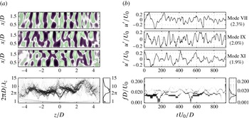
From mode VII, all spatial POD modes involve broader-banded dynamics with non-trivial spatial structures. Modes VII, IX and XI are presented in figure 17 as examples of such features. They exhibit multiple patterns distributed over the entire span and characterised by large variations of spanwise wavenumbers in the range
 $3\lesssim {\it\beta}\lesssim 13$
. Consistently, the temporal modes present diverse time scales in the range
 $0.002\lesssim f\,D/U_{0}\lesssim 0.03$
. These POD modes probably participate in the inner-flow dynamics deriving from centrifugal instabilities and modulating the shear layer oscillations.
Until now, the study has focused on identifying and characterising the slow dynamics responsible for the severe AM of the shear layer self-sustained oscillations. The analysis has demonstrated that the very low modulating frequencies are associated with three-dimensional coherent structures resulting from centrifugal instabilities. This dynamics organises as slow-moving spanwise-travelling helical waves which arise within the inner flow and yield a wavelength
 ${\it\lambda}_{z}\approx D$
. The way in which these three-dimensional waves interact nonlinearly with the shear layer vortex shedding is studied in detail in the next section.
5. Nonlinear coupling with inner-flow 3D waves
The focus of the analysis that follows is now on the coupling mechanism linking inner-flow spanwise waves to shear layer AMs. As shear layer oscillations and centrifugal instabilities evolve over very different time scales, the connection can be investigated by separating the fast from the slow dynamics of the flow.
5.1. Scale separation
The flow is split according to the two aforementioned time scales: CI, frequencies consistent with centrifugal instabilities, in the range of expression (1.3); and SL, the locked-on frequencies of the shear layer, verifying (1.1). The latter scale corresponds to carrier frequencies of the amplitude-modulated oscillations. Therefore, it must be demodulated so as to extract the envelope. The envelope is then discussed with regards to the three-dimensional waves inside the cavity so as to characterise the nonlinear interactions between shear layer waves and centrifugal instabilities. Scale separation is utilised in the (
 $x,y$
)- and (
 $z,x$
)-planes under investigation to reconstruct the low-frequency dynamics of the inner flow on one hand and the shear layer dynamics on the other hand.
5.1.1. Proper orthogonal decomposition partial reconstruction in the (
$z,x$
)-plane

Proper orthogonal decomposition avails us to reconstruct part of the dynamics considering only a few relevant modes. The reconstructed space–time dynamics is obtained from
 $$\begin{eqnarray}R(\boldsymbol{x},t)=\unicode[STIX]{x1D650}\times \unicode[STIX]{x1D64E}\times \unicode[STIX]{x1D651}^{\text{T}},\end{eqnarray}$$
where
 $\unicode[STIX]{x1D650}$
and
 $\unicode[STIX]{x1D651}$
are the unitary matrices containing respectively the spatial and temporal signatures of the selected POD modes and
 $\unicode[STIX]{x1D64E}$
is the diagonal matrix containing the associated singular values. In the following,
 $R_{SL}(z,x,t)$
is the reconstruction using modes
 $\{\text{I,VI}\}$
corresponding to shear layer dynamics while
 $R_{CI}(z,x,t)$
uses modes
 $\{\text{II}{-}\text{V},\text{VII}{-}\text{XI}\}$
so as to contain the dynamics derived from centrifugal instabilities.
5.1.2. Spectral filtering in the (
$x,y$
)-plane

Unlike the (
 $z,x$
)-plane, the POD modes computed from the (
 $x,y$
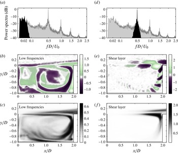
)-plane – in § 4.1 – do not strictly separate the two time scales. Spectral filtering is here preferred to separate the low-frequency range from the self-sustained oscillations. Butterworth filters of order 4 are applied to the time series throughout the fluctuating fields, as illustrated in figure 18.
Time-filtered vorticity fluctuations in an (
 $x,y$
)-plane, for
 $L/D=2.0$
and
 $L/{\it\theta}_{0}=82$
. (a–c) Low-pass to keep centrifugal instabilities only,
 $R_{CI}(x,y,t)$
. (d–f) Band-pass around the dominant shear layer frequency,
 $R_{SL}(x,y,t)$
. (a,d) Power spectra. (b,e) Examples of filtered snapshots. (c,f) Vorticity r.m.s.

First, low-pass filtering is used with a cutoff frequency
 $f_{c}\,D/U_{0}=0.07$
, so as to encompass the low-frequency broad-band peak (figure 18
a) corresponding to the reconstructed dynamics,
 $R_{CI}(x,y,t)$
. The filtered snapshot and root mean square (r.m.s.) distribution in figure 18(b,c) render the inner-flow dynamics wrapped around the main recirculation characteristic of centrifugal instabilities.
Second, a band-pass filter is applied to remove all time scales apart from the carrier frequency of the self-sustained oscillations. In the example shown in figure 18(d), the filtered spectrum only shows significant energy around the (dominant) locked-on frequency –
 $f_{a}\,D/U_{0}\simeq 0.5$
in figure 18. As expected, the reconstructed dynamics
 $R_{SL}(x,y,t)$
is restricted to the shear layer flapping motion. The filtered snapshot in figure 18(e) depicts shear layer oscillations and, to a lesser extent, inflows along the downstream wall of the cavity. This is confirmed by the high r.m.s. levels in the impingement region, leaving the inner flow basically free of high frequency dynamics (figure 18
f).
5.2. Amplitude modulation by spanwise waves
The AM of the self-sustained oscillations is analysed with respect to the spanwise waves inside the cavity. Cross-correlations are used to ascertain the prominent effect of the inner-flow centrifugal instabilities on the shear layer oscillations throughout the parameter range investigated.
5.2.1. Envelope of the shear layer waves
Once the shear layer dynamics is reconstructed in
 $R_{SL}$
, one obtains an amplitude-modulated signal consisting of a carrier – the locked-on (high) frequency – and an envelope. Application of the Hilbert transform to every zero-mean time series extracted across the (
 $z,x$
)-plane enables us to construct an analytic (complex) signal, whose instantaneous amplitude represents the envelope of the self-sustained oscillations. As this envelope reveals the AM of shear layer oscillations, it will be referred to as
 $R_{AM}(\boldsymbol{x},t)$
.
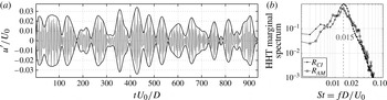
The extraction of
 $R_{AM}(\boldsymbol{x},t)$
is illustrated in figure 19(a) for the case
 $\mathit{Re}_{D}=2400$
,
 $L/{\it\theta}_{0}=59$
,
 $L/D=2$
, already investigated in § 4.2. The HHT is applied to the time series of both
 $R_{AM}$
and
 $R_{CI}$
in order to obtain the instantaneous dominant frequencies involved in both the shear layer modulations and the slow dynamics. The resulting marginal spectra plotted in figure 19(b) are integrated both in the spanwise position and over time. Both
 $R_{AM}$
and
 $R_{CI}$
exhibit a unique salient Strouhal number at 0.015. It corresponds to the central frequency of the two counter-travelling spanwise waves – depicted by the POD modes II–V – associated with frequencies of 0.014 and 0.016. The match between the spectral contents of
 $R_{AM}$
and those of
 $R_{CI}$
demonstrates once more the prominent influence of inner-flow centrifugal instabilities on the AM.
Temporal dynamics of the amplitude of the shear layer oscillations for the case
 $L/{\it\theta}_{0}=59$
,
 $L/D=2$
,
 $\mathit{Re}_{D}=2400$
. (a) Time series
 $R_{SL}(z=3\,D,x=1.84\,D,t)$
extracted from shear layer reconstructed dynamics near the impingement, along with the associated envelope
 $R_{AM}(z=3\,D,x=1.84\,D,t)$
. (b) Hilbert–Huang marginal (integrated) spectra of both the shear layer envelope
 $R_{AM}$
and the slow dynamics
 $R_{CI}$
are confronted.

5.2.2. Modulating dynamics
The role of the inner-flow centrifugal instabilities as modulating dynamics of the shear layer waves is consistently recovered for different control parameters. This assertion is notably confirmed by the temporal correlations of the time series resulting from
 $R_{AM}$
and
 $R_{CI}$
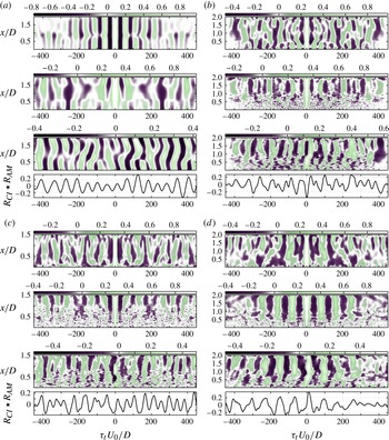
along the shear layer. Four different parametric cases are presented in figure 20. Salient features are common to all cases despite the increasing complexity with larger control parameters
 $\mathit{Re}_{D}$
and
 $L/{\it\theta}_{0}$
. The auto-correlation of both
 $R_{CI}$
and
 $R_{AM}$
consistently depicts a fairly periodic signature involving similar time scales, see figure 20(a–d) (top, middle). As expected, the associated frequencies are characteristic of centrifugal instabilities (1.3). Even more remarkable are the high correlation levels in
 $R_{CI}\star R_{AM}$
– see figure 20(a–d) (bottom) – even over large time horizons. These high cross-correlations corroborate the close connection between inner-flow centrifugal instabilities and the modulated dynamics of the shear layer waves.
Time cross-correlations computed from streamwise velocity fluctuations
 $u^{\prime }/U_{0}$
along
 $x$
at
 $y=-0.1\,D$
close to mid-span in the reconstructed dynamics
 $R_{CI}$
and
 $R_{AM}$
, for four experimental cases. For each case and from top to bottom, auto-correlation
 $R_{CI}(x,t)\star R_{CI}(x,t)$
, auto-correlation
 $R_{AM}(x,t)\star R_{AM}(x,t)$
, cross-correlation
 $R_{CI}(x,t)\star R_{AM}(x,t)$
and extraction
 $R_{CI}(x=0.75\,L,t)\star R_{AM}(x=0.75\,L,t)$
. (a)
 $\mathit{Re}_{D}=2400,L/{\it\theta}_{0}=59,L/D=2,S/D=10$
. (b)
 $\mathit{Re}_{D}=4550,L/{\it\theta}_{0}=82,L/D=2,S/D=6$
.(c)
 $\mathit{Re}_{D}=7470,L/{\it\theta}_{0}=79,L/D=1.5,S/D=6$
. (d)
 $\mathit{Re}_{D}=5750,L/{\it\theta}_{0}=91,L/D=2,S/D=6$
.

Nevertheless, modulating and modulated dynamics evolve slightly differently throughout the parameter space. The case shown in figure 20(a) presents a large spanwise extension and a small dimensionless cavity length
 $L/{\it\theta}_{0}$
. The reconstructed dynamics
 $R_{CI}$
is highly coherent and uniformly correlated along the cavity length. The spanwise waves derived from centrifugal instabilities hereby prevail over the modulated dynamics of the shear layer
 $R_{AM}$
. In contrast, the case seen in figure 20(d) corresponds to a higher Reynolds number and a higher dimensionless cavity length, with a smaller cavity span. These control parameters promote the self-sustained oscillations of the shear layer over inner-flow spanwise waves. As a result,
 $R_{AM}$
shows a quasi-periodic temporal signature while the centrifugal instabilities depicted by
 $R_{CI}$
appear to be strongly distorted. In spite of this change in the prevalence of the two coexisting phenomena, the time cross-correlation
 $R_{CI}\star R_{AM}$
remains high and basically periodic for all the investigated control parameters, as shown in figure 20(a–d) (bottom). The AMs of the shear layer waves remain strongly time correlated with the slow dynamics of the inner flow.
5.2.3. Spanwise versus temporal modulation
Considering the three-dimensional structure of the modulating dynamics, the question arises as to how the AM organises along the span of the cavity. The envelope of the shear layer either exhibits spanwise modulations bound to inner-flow centrifugal instabilities, or remains mainly two-dimensional like its carrier waves. To address this question we consider the spanwise correlations of the flow.
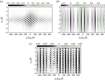
Two-dimensional correlations of spanwise–time reconstructed dynamics, extracted at
 $(x,y)=(1.84\,D,-0.1\,D)$
for the case
 $L/{\it\theta}_{0}=59$
,
 $L/D=2$
,
 $\mathit{Re}_{D}=2400$
: (a) auto-correlation
 $R_{CI}\star R_{CI}$
; (b) auto-correlation
 $R_{AM}\star R_{AM}$
; (c) cross-correlation
 $R_{CI}\star R_{AM}$
. Distributions are normalised and
 $\{{\it\tau}_{t},{\it\tau}_{z}\}$
are the time and spanwise delays, respectively.

Two-dimensional (
 $z,t$
)-correlations are computed for both
 $R_{CI}(t,z)$
and
 $R_{AM}(t,z)$
reconstructed dynamics in figure 21. The auto-correlation of
 $R_{CI}(t,z)$
in figure 21(a) depicts a chessboard-like structure formed by crossing stripes of alternate correlation. This distribution represents the interference patterns produced by the superimposition of the two dominant counter-travelling spanwise waves. The positive slope corresponds to the right-travelling wave and the negative slope to the left-travelling wave. This salient characteristic of the cavity inner flow has already been reported in Douay et al. (Reference Douay, Guéniat, Pastur, Lusseyran and Faure2011), Basley (Reference Basley2012) and de Vicente et al. (Reference de Vicente, Basley, Meseguer-Garrido, Soria and Theofilis2014). Such an interference is commonly encountered when dealing with centrifugal instabilities. It is worth remarking that the space–time signature of the reconstructed dynamics
 $R_{CI}(t,z)$
constitutes a (quasi) standing wave. It can therefore be modelled as the idealised form
 $$\begin{eqnarray}R_{CI}(t,z)\sim A_{sw}\sin (2{\rm\pi}\mathit{St}_{sw}\,t^{\prime })\cos ({\it\beta}_{sw}\,z^{\prime }),\quad \text{with}\ t^{\prime }=t\,U_{0}/D,\ z^{\prime }=z/D.\end{eqnarray}$$
The frequency
 $\mathit{St}_{sw}$
and the wavenumber
 ${\it\beta}_{sw}$
depend on the underlying counter-travelling waves. In the present case, one obtains
 $\mathit{St}_{sw}=2{\rm\pi}(\mathit{St}_{\leftarrow }+\mathit{St}_{\rightarrow })/2\simeq 0.015$
and
 ${\it\beta}_{sw}=({\it\beta}_{\leftarrow }-{\it\beta}_{\rightarrow })/2\simeq 2{\rm\pi}$
. This depicts spanwise oscillations of wavelength
 $D$
with a beating of the average Strouhal number
 $\mathit{St}_{sw}=0.015$
, consistent with figures 19(b) and 21(a).
On the other hand, the auto-correlation of the envelope
 $R_{AM}(t,z)$
remains two-dimensional with no discernible spanwise scales observed in figure 21(b). This indicates that the self-sustained oscillations are alternately enhanced and damped simultaneously everywhere along the span, translating into a strictly temporal AM. This separation between the spanwise waves of the inner flow and the envelope of the shear layer is confirmed by the particularly low (
 $z,t$
) cross-correlations
 $R_{CI}\star R_{AM}$
, shown in figure 21(c). Inner-flow centrifugal instabilities do not influence local vortex shedding. The coupling mechanism responsible for the AMs rather appears to be global. The beating implied by the standing wave of
 $R_{CI}$
dynamics could be related to this coupling mechanism since it represents a temporal cycle, which is globally undergone by the inner flow. Such a swell might temper the impingement of the vortices shed along the shear layer. Self-sustained oscillations would hence be alternately damped and enhanced as the shear layer respectively avoids or impinges on the trailing edge of the cavity.
6. Concluding remarks
This study brings to light the occurrence of severe AMs of the shear layer waves developing in open cavity flows. The focus is on the lowest modulating frequencies, broad band and typically down to two orders of magnitude below the locked-on frequencies of the shear layer. Amplitude modulations by such very low frequencies are observed consistently and for a wide range of control parameters. The analysis demonstrates that they result from the influence of centrifugal instabilities along the recirculating inner flow. Indeed, this work constitutes one of the few extensive studies dealing with the coexistence of shear layer self-sustained oscillations and centrifugal instabilities in open cavity flows.
The onset of centrifugal instabilities along the recirculating flow leads to slow-moving 3D dynamics, whose most salient features are pairs of counter-propagating spanwise waves. The overlap of these spanwise waves induces interference patterns. In terms of coherent structures, the inner-flow dynamics consists of alleys of spiral vortices pulsating and coiling up around the main recirculation.
The analysis reveals that the inner-flow temporal dynamics and shear layer AMs are highly correlated. Indeed, the bicoherence spectra show that the very-low-frequency 3D waves resulting from centrifugal instabilities exchange significant energy with the locked-on waves of the shear layer through quadratic nonlinearities. It is particularly remarkable that such coherent spanwise fluctuations endure and continue to influence the high-frequency dynamics of the shear layer despite the increasing strength of the vortex shedding.
The severe temporal modulations of the self-sustained oscillations do not correspond to spanwise modulations: the envelope, modulated in time, remains fairly two-dimensional. It appears that the 3D waves of the inner flow interfere with each other to induce a global modulation of the flow. The notion of a swell is here proposed to refer to a cycle of alternate enhancing/damping of the self-sustained oscillations. Further investigations are necessary to shed more light on the global nature of this coupling mechanism.
Acknowledgements
This work has been supported by Direction Generale de l’Armement and Agence Nationale de la Recherche (project ANR-06-BLAN-0363). The authors would also like to acknowledge the support of this research by the Australian Research Council.