

Introduction
Green Peafowl Pavo muticus are restricted to the open dry forest habitats of Southeast Asia (Sukumal et al. Reference Sukumal, Dowell and Savini2017). They are classified as Endangered due to their population decline following hunting and extensive habitat degradation and loss over the past decades (BirdLife International 2021). Long-term viable populations have been predicted to be found in six strongholds containing sufficiently large habitat over the historical range of the species (Sukumal et al. Reference Sukumal, Dowell and Savini2020). In Myanmar, the only confirmed stronghold is in the Bago Yoma range, where an estimated population density of 0.825 calling males per km2 was recorded in dry dipterocarp forest and 0.866 calling males per km2 in large-scale teak plantations (Win et al. Reference Win, Sukumal, Shwe and Savini2023). However, additional populations are reported to be scattered across the country, often found in small fragments of natural habitat. The species also makes extensive use of the surrounding agricultural landscape, where it is culturally significant and tolerated by farmers (Shwe et al. Reference Shwe, Sukumal, Oo, Dowell, Browne and Savini2021).
Due to its geographical location, Myanmar shows large habitat diversity supporting rich biodiversity (Wikramanayake et al. Reference Wikramanayake, Dinerstein, Loucks and Olson2001). Due to uncertain political situations over the last decades, the country has recorded one of the most extensive habitat losses worldwide (FAO 2015), with the forested area shrinking by 6.6% from 2005 (366,248 km2) to 2016 (342,106 km2), representing a forest loss of 0.62% per year (Reddy et al. Reference Reddy, Unnikrishnan, Asra, Manikandan and Jaishanke2019a). This habitat loss, combined with extensive illegal hunting and wildlife trade, has resulted in an extensive decline in biodiversity, drastic for several species (Reddy et al. Reference Reddy, Pasha, Satish, Unnikrishnan, Chavan and Jha2019b). To reduce habitat and biodiversity loss, a decade or more ago Myanmar established additional protected areas and improved the existing ones (MOECF 2015). Unfortunately, in recent years the management of protected areas has declined due to the deterioration of the security situation. However, forest cover in and around protected areas has declined less than in non-protected forests (Biswas et al. Reference Biswas, Vadrevu, Lwin, Lasko and Justice2015), indicating that protected areas in Myanmar are, or at least were, not exclusively ‘paper parks’ as initially suggested (Aung Reference Aung2007). Protected areas have therefore proven to be an effective tool for the management and conservation of biodiversity (Coad et al. Reference Coad, Leverington, Burgess, Cuadros, Geldmann and Marthews2013), with their effectiveness assessed by monitoring the status of indicator species for the different habitats found within (Dale and Beyeler Reference Dale and Beyeler2001).
In this regard, several nature reserves have been established in the country over the past decade. Among those, the Indawgyi Biosphere Reserve was designated in 2017 with the purpose of protecting the intact forest surrounding the Indawgyi Lake (Than Reference Than2017). To support effective management, the population of resident eastern hoolock gibbons Hoolock leuconedys has been estimated at a fine scale across the entire reserve (Lwin et al. Reference Lwin, Ngoprasert, Sukumal, Browne and Savini2022). This species serves as an indicator of forest integrity, as individuals are confined to pristine forest, which is essential both for moving between connected high tree canopies and for sustaining their frugivorous diet (Lwin et al. Reference Lwin, Sukumal and Savini2021). Furthermore, due to their monogamous social structure, the population is highly sensitive to hunting. However, this species is not suitable for assessing the conservation status of open grassland habitats along lake and river shorelines. To address this problem, efforts should focus on estimating the Green Peafowl population recently discovered in the open habitats surrounding the lake shores, given that Galliformes are considered good indicators of habitat conservation status (Savini et al. Reference Savini, Namkhan and Sukumal2021).
It is therefore the aim of this work to estimate the Green Peafowl population in the Indawgyi Biosphere Reserve using Distance sampling from data collected along line transects, as has been extensively done for the species (Sukumal et al. Reference Sukumal, McGowan and Savini2015). Use an infinite-weight logistic regression model (Hefley and Hooten Reference Hefley and Hooten2015) to define the specific habitat used by the species by using as it appears to occupy a different habitat from the well-known dry dipterocarp forest. In the end, the estimated densities will inform the development of a more accurate management plan for the open habitats of the Biosphere Reserve.
Study site and Methods
Field site
Indawgyi Biosphere Reserve, Kachin State, covers a total area of 1,337 km2 (Figure 1). A totally protected forest core zone of 423 km2, where access and the harvesting of forest products are forbidden, is covered by deciduous, mixed deciduous, mixed evergreen, and evergreen forests. The remaining 914 km2 consists of a buffer zone, where sustainable use of forest products and fishing is allowed, and a transition zone, where human settlement and sustainable agriculture are found. The Reserve’s elevation ranges between 180 and 1,180 m asl (MONREC 2017). Temperatures average 33.6°C in the hottest months (Mar-May) and 8.5°C in the coldest months (Dec-Jan). Rainfall ranges between 1,048 and 2,060mm (Mohnyin weather station data from 2019).
The study site within the Indawgyi Biosphere Reserve, showing the core zone (dark green polygon), buffer zone (light green polygon), and transition zone (buff-colored polygon). The locations of the 2 km transects are also shown.

Figure 1. Long description
A topographical map displays the Indawgyi Biosphere Reserve divided into three colored regions. The core zone is represented by dark green polygons, primarily concentrated in the East and Southwest. The buffer zone is shown in light green, forming a central vertical corridor and smaller patches. The transition zone is a large buff-colored polygon covering the North and central-West areas.
Numbered transects, indicated by red lines with green circular endpoints, are distributed across the zones.
* In the North within the transition zone, transect 51 to 52 is isolated.
* In the Northeast, a cluster of transects includes 22 to 21, 32 to 31, 61 to 62, 12 to 11, and 42 to 41.
* In the central region, transect 71 to 72 sits on the border between the transition and core zones.
The map includes topographical features like the Mohnyin District label, river names such as Namyin Chaung and Hwenka Hka, and elevation markers like 1546 m and 1328 m. A legend at the bottom right identifies the Buffer, Core, and Transition zones. Attribution to Esri, NASA, N G A, and U S G S is provided at the bottom.
The Biosphere Reserve was established in 2017 to protect the area’s unique ecosystems and biodiversity. Prior to its establishment, villages had existed in the region between 1688 and 1989, developing rice farming as their main livelihood (Latt Reference Latt2009) while also relying on timber, firewood, and non-timber forest products for local consumption. For 20 years leading up to 1999, the forest was logged by the Myanmar Timber Enterprise, after which a wildlife sanctuary was created to provide formal protection (MONREC 2018). Despite these conservation efforts, recent activities, including illegal gold mining between 2012 and 2017, have impacted the southwestern part of the Reserve, causing extensive deforestation (MONREC 2018).
Estimating Green Peafowl density
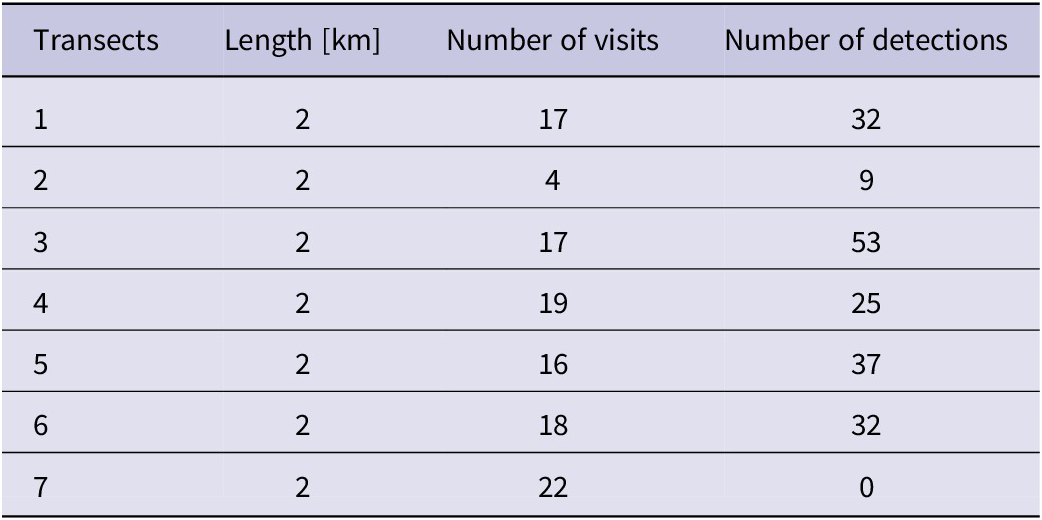
Green Peafowl density was estimated using DISTANCE version 7.3 from data collected along line transects. A total of seven 2-km transects were laid in the area immediately north of the Indawgyi Lake along the river that drains out of the lake. The surrounding vegetation is characterised by open woodland, grassland, and rice fields (Figure 1). The presence of the species in this area has been documented in previous surveys conducted by other research groups and corroborated by reports from local farmers. Transects were spaced at a minimum distance of 1,300 m to ensure independence.
Each of the transects was surveyed over a four-month period, between January and April 2022. Due to security issues in some parts of the reserve, each transect was surveyed between 4 and 18 times over the study period (see Table 1 and Table S1 for details of the survey effort for each transect). Repeated surveys at each transect were carried out monthly over the whole survey period to maintain a similar calling rate over the whole survey. Independence of calling between different visit was controlled by including survey effort in the analysis. Surveys were conducted in the morning between 06:00 and 08:00 and once in the afternoon between 16:00 and 18:00. During each survey, the angle to both visual sightings and auditory detections was estimated using a compass and recorded. To prevent double counting along a transect, each detection was examined for spatial overlap with other detections recorded on the same transect.
Details of transects established around the Indawgyi Biosphere Reserve area.
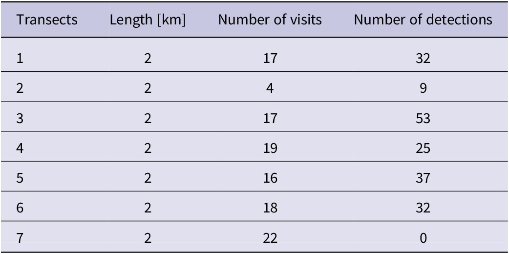
Table 1. Long description
The table consists of four columns and seven data rows.
* Column 1: Transects (numbered 1 through 7).
* Column 2: Length in k m (all transects are 2 k m long).
* Column 3: Number of visits.
* Column 4: Number of detections.
Data breakdown by row:
* Transect 1: 17 visits, 32 detections.
* Transect 2: 4 visits, 9 detections.
* Transect 3: 17 visits, 53 detections.
* Transect 4: 19 visits, 25 detections.
* Transect 5: 16 visits, 37 detections.
* Transect 6: 18 visits, 32 detections.
* Transect 7: 22 visits, 0 detections.
To compare our density estimates to what mostly available in the literature we used only calling males detection to estimate the density. Density estimation on individual transects was not performed, as the number of acoustic detections per transect was below the minimum threshold of 40 detections required for reliable density estimation using DISTANCE (Buckland et al. Reference Buckland, Anderson, Burnham, Laake, Borchers and Thomas2001). Consequently, density was estimated by pooling data across all transects. To select the best detection function, key models including half-normal, hazard rate, and negative exponential functions with a series of adjustments (cosine, simple polynomial, and Hermite polynomial) were examined, and the model with the lowest AIC was chosen following Buckland et al. (Reference Buckland, Anderson, Burnham, Laake, Borchers and Thomas2001).
Defining habitat used by Green Peafowl
The habitat utilised by the Green Peafowl in the Biosphere Reserve was modelled using presence-only data obtained from species occurrence records collected along line transects. A total of 188 initial locations was collected from six transects. Redundancy between adjacent points was eliminated by creating 282 m radius buffers around each record. When two or more buffers overlapped by more than 5%, only one was retained after being selected randomly (Sukumal et al. Reference Sukumal, Dowell and Savini2020). The 282 m radius buffer was based on the reported 25 ha home range size of male radio-tagged Green Peafowl during the breeding season (Sukumal et al. Reference Sukumal, Dowell and Savini2017), resulting in 56 independent ‘used’ locations. Available habitat was defined by randomly selecting 949 points within a rectangular area covering all transects, using the ‘Create Random Point’ tool in ArcGIS Pro 3.3.0 (Esri, 2024). These random points were spaced at a minimum distance of 564 m (twice the 282-m radius) to ensure independence. As for the used points, a 282 m radius buffer was centred on each point. This sampling approach guarantees representative coverage of environmental variation when using a presence-availability model (Barbet-Massin et al. Reference Barbet-Massin, Jiguet, Albert and Thuiller2012). We measured the degree of spatial autocorrelation between both used and random locations to verify the spatial independence of each sample, using Moran’s I statistic (Moran 1950). A non-significant Moran’s I value (P > 0.05) indicates that points are randomly distributed in space, satisfying the independence requirement for habitat modelling (Dormann et al. Reference Dormann, McPherson, Araújo, Bivand, Bolliger and Carl2007).
Habitat types within each used and random buffers were obtained from the Climate Change Land Cover dataset for the year 2015, downloaded from http://maps.elie.ucl.ac.be/CCI/viewer/download.php. The original dataset contained 37 habitat types. We eliminated unsuitable habitats, such as bare areas, urban areas, and water bodies, and reclassified the remaining 19 habitat types within the study range into 16 major habitat types (Supplementary Material Table S2).
Habitat selection models were constructed using an infinite-weight logistic regression model (Hefley and Hooten Reference Hefley and Hooten2015) to investigate the relationship between habitat covariates and the probability of occurrence based on used and available points. Used locations were based on 56 independent presence-only records collected along transects. Available points were randomly generated within a rectangular area covering all transects (see details above). Before running the analysis, each habitat covariate was standardised by subtracting its mean and dividing it by its standard deviation using the ‘scale’ function in program R (R Core Team 2025). All habitat covariates were assessed for multicollinearity using pairwise Kendall’s τ correlations. When any pair of covariates had a correlation coefficient greater than 0.5, one was excluded from the model. All data were evaluated for outliers and overdispersion using the DHARMA package (Harting Reference Harting2019). A constant model (intercept-only without covariates) and a set of models containing covariates were fitted and compared using Akaike Information Criterion (AIC) and AIC weights. The best model was selected based on the lowest AIC value and highest AIC weight. We also used the area under the curve (AUC) to evaluate the best model, with AUC values of 0.7-0.8 indicating acceptable model performance, 0.8-0.9 indicating excellent performance, and values >0.9 indicating outstanding performance. All statistical analyses were conducted using R software (R Core Team 2025).
Results
Estimated Green Peafowl density
A total of 188 independent detections were recorded over the survey period across six transects, while no detections were recorded on one transect (see Table 1 for details).
The overall estimated density (global estimated density) across the six transects was 0.68 calling birds km−2 (95% CI=0.47-0.97). Five of the six established transects were located in the northeastern section of the study site which was characterised by suitable open forest and 150 calling birds were detected. The bird density in this area was estimated at 0.51 calling birds km−2 (95% CI=0.31-0.82) (Table 2).
Estimated Green Peafowl density across all six transects (global estimate) and within the five transects in the northeast section.

Table 2. Long description
The table consists of eight columns and two data rows.
Columns from left to right are:
1. Site.
2. Number of transect.
3. Total transect length in k m.
4. Total walking distance in k m.
5. Total number of detections.
6. Density estimates.
7. 95 percent confidence intervals.
8. percent C V.
Data Row 1: Global estimate.
- Number of transect: 6.
- Total transect length: 12 k m.
- Total walking distance: 182 k m.
- Total number of detections: 188.
- Density estimates: 0.68 calling birds per k m super 2.
- 95 percent confidence intervals: 0.47 to 0.97.
- percent C V: 15.83.
Data Row 2: Northeast section.
- Number of transect: 5.
- Total transect length: 10 k m.
- Total walking distance: 150 k m.
- Total number of detections: 151.
- Density estimates: 0.51 calling birds per k m super 2.
- 95 percent confidence intervals: 0.31 to 0.82.
- percent C V: 17.39.
Habitat used
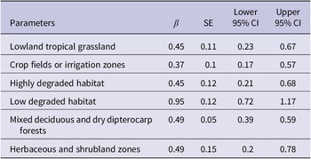
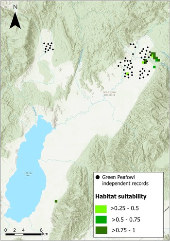
The best model (based on the lowest AIC), which exhibited an AUC of 0.87, showed a positive correlation between the probability of occurrence and the following six covariates: lowland tropical grassland, crop fields or irrigation zones, highly degraded habitat, low degraded habitat, mixed deciduous and dry dipterocarp forests, and herbaceous and shrubland zones (Table 3). The predicted remaining suitable habitats, defined using a probability of occurrence ranging between gradient 0.25 and 1 divided in three classes (>0.25–0.5, >0.5–0.75 and >0.75 to 1) based on the best model, occurred overall as very small fragmented patches within the study site and covered an area of 0.69 km2, 0.46 km2 and 2.07 km2 respectively (Figure 2). We excluded the probability of occurrence below 0.25 as those values highlighted the whole study area as suitable, making the result meaningless.
Habitat covariates in the best-fitting model influencing Green Peafowl occurrence probability.
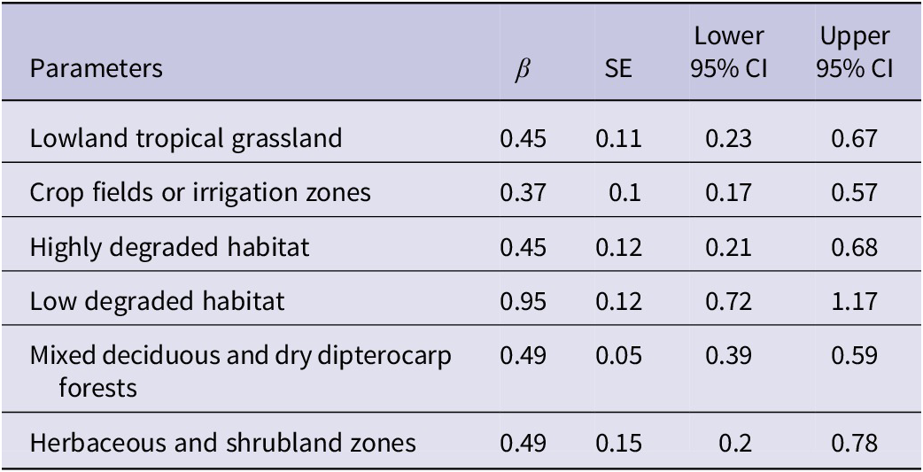
Table 3. Long description
The table consists of five columns: Parameters, beta (represented by the Greek letter beta), S E, Lower 95 percent C I, and Upper 95 percent C I.
* Lowland tropical grassland: beta 0.45, S E 0.11, Lower 95 percent C I 0.23, Upper 95 percent C I 0.67.
* Crop fields or irrigation zones: beta 0.37, S E 0.1, Lower 95 percent C I 0.17, Upper 95 percent C I 0.57.
* Highly degraded habitat: beta 0.45, S E 0.12, Lower 95 percent C I 0.21, Upper 95 percent C I 0.68.
* Low degraded habitat: beta 0.95, S E 0.12, Lower 95 percent C I 0.72, Upper 95 percent C I 1.17.
* Mixed deciduous and dry dipterocarp forests: beta 0.49, S E 0.05, Lower 95 percent C I 0.39, Upper 95 percent C I 0.59.
* Herbaceous and shrubland zones: beta 0.49, S E 0.15, Lower 95 percent C I 0.2, Upper 95 percent C I 0.78.
Predicted suitable habitat for Green Peafowl occurrence (probability ranging between 0.25 and 1) based on the best-fitting model.
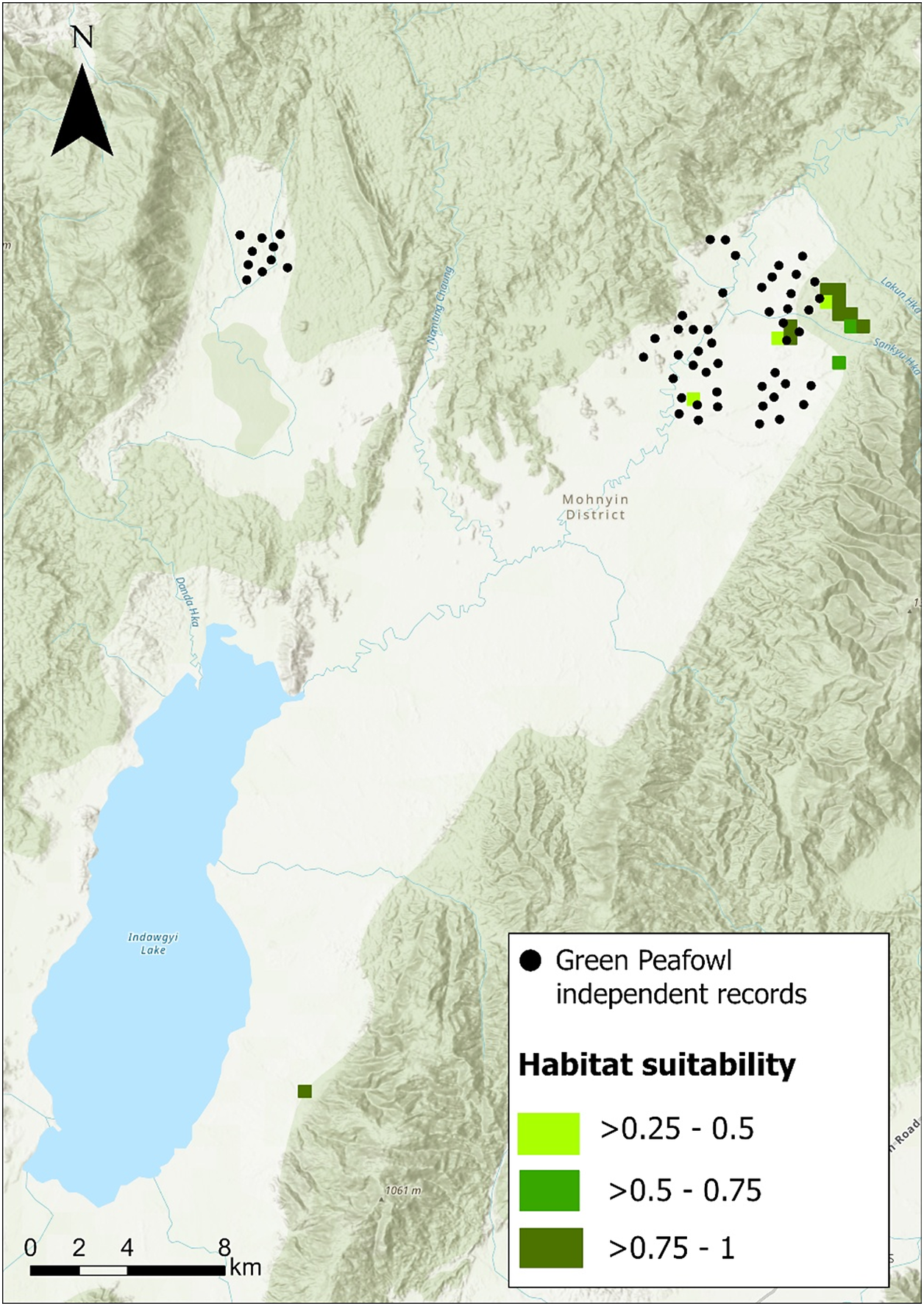
Figure 2. Long description
A topographical map of the Mohnyin District featuring Indawgyi Lake in the Southwest. A North arrow is located in the Top-Left corner and a scale bar of 0 to 8 k m is at the Bottom-Left.
Data distribution:
* Black dots representing Green Peafowl independent records are clustered in two main areas: a smaller group in the Northwest and a larger, denser cluster in the Northeast.
* Habitat suitability is indicated by green shaded squares. Light green represents greater than 0.25 to 0.5 probability. Medium green represents greater than 0.5 to 0.75 probability. Dark green represents greater than 0.75 to 1 probability.
* The highest suitability (dark green) is concentrated on the Eastern edge of the Northeast cluster, near the Sankyu Hka river.
* A single medium green square is located South of the lake near a mountain peak labeled 1061 m.
Geographical features include:
* Indawgyi Lake, a large blue body of water in the Southwest.
* Rivers including Danda Hka, Namting Chaung, Lakun Hka, and Sankyu Hka.
* Terrain is characterized by light green and tan shaded relief indicating mountainous ridges and valleys.
Discussion
The estimated density of Green Peafowl in the area north of Indawgyi Lake, ranged between 0.51 and 0.68 calling males per km2. Those densities have been estimated by pooling detections from all transects as densities for each transect could not be estimated due to low detections. Therefore, due to detection heterogeneity between the transects, the result does not represent an equal density per transect. These densities are particularly low when compared to other non-protected areas in Myanmar that are partially covered by agricultural land surrounding natural habitats. A similar low density was estimated in unprotected natural dry forest habitat (0.82 calling males per km2) and in large areas of teak plantations (0.87 calling males per km2) along the western side of the Bago Yoma range (Win et al. Reference Win, Sukumal, Shwe and Savini2023). In contrast, on the Shan Plateau, Green Peafowl density was estimated at 1.13–2.63 calling males per km2 in areas comprising low-intensity multi-crop agricultural landscapes and lightly-degraded fallow land surrounding small fragments of natural habitat protected by a monastery that actively managed the area (Shwe et al. Reference Shwe, Sukumal, Oo, Dowell, Browne and Savini2021). The low density recorded could be a combination of different issues. First, most of the detections were collected outside the boundaries of the Biosphere Reserve. Two transects were in the buffer, two in the transition zone the rest in the surrounding agricultural areas following known peafowl locations. This suggests a low protection with species facing threat from degradation and hunting. Second, the population is recorded to inhabit open woodland, grassland, and rice fields near human activities such as agriculture and farming. Those habitats differ from the Dry Dipterocarp Forest inhabited usually by the species (Sukumal et al. Reference Sukumal, Dowell and Savini2020) which could indicate a certain adaptation level to a less optimal habitat which however has shown to result in lower density (Win et al. Reference Win, Sukumal, Shwe and Savini2023).
Ongoing threats and disturbance levels can negatively impact the long-term survival of the species (Sukumal et al., Reference Sukumal, Dowell and Savini2020). For instance, in Yok Don National Park (southcentral Vietnam), high threats in the form of fire, hunting, and domestic livestock overgrazing resulted in densities as low as 0.25 calling male km−2 despite the dry forest habitat being considered suitable (Sukumal et al. Reference Sukumal, McGowan and Savini2015). Similarly, in northwestern Thailand, Green Peafowl density was low (0.27 calling males per km2) as most of the habitat showed varying levels of degradation due to nearby human settlements (Sukumal et al. Reference Sukumal, Thunhikorn and Savini2023).
Despite the relatively low estimated density, the sites surveyed around the Indawgyi Biosphere Reserve can still be considered important for the long-term conservation of this Endangered species, as they border protected natural habitat and may receive at least some level of management.
The site shows an overall small extent of suitable habitat for Green Peafowl, with only 3.22 km2 predicted to have a probability of occurrence ranging between 0.25 and 1 (Figure 2). The species appears to be distributed mostly in less optimal habitat surrounding the suitable habitat, suggesting a certain degree of flexibility in habitat use, likely linked to the limited availability of optimal habitat. Adaptation to sub-optimal agricultural landscapes and degraded forests, particularly when adjacent to fragments of natural habitat, has been reported in several peafowl populations. On the Shan Plateau, Green Peafowl are found in low-intensity agricultural areas surrounding a small patch of natural habitat (0.23 km2), far too small to maintain the population present (Shwe et al. Reference Shwe, Sukumal, Oo, Dowell, Browne and Savini2021). This adaptation is likely driven by the small-scale, multi-crop nature of the farmland, which provides the species with regular food sources. A similar explanation has been proposed for the high-density population (up to 13.47 calling males per km2) recorded in the farmland of northern Thailand (Saridnirun et al. Reference Saridnirun, Sukumal, Grainger and Savini2023). In this case, however, the natural habitat comprised a large protected area, and the surrounding crops were a mosaic of paddy fields and orchards that provided vegetation structure sufficiently similar to the natural habitat.
Green Peafowl have shown resilience and relatively rapid recovery when populations are effectively managed and threats are reduced. In Huai Kha Kaeng Wildlife Sanctuary, western Thailand, improved management increased estimated density to 11.34 calling males per km2 (Sukumal et al. Reference Sukumal, Dowell and Savini2017). In Cat Tien National Park, southern Vietnam, where habitat conditions are also suboptimal, densities rose from 1.31 to between 3.02 and 4.69 calling males per km2 (Sukumal et al. Reference Sukumal, McGowan and Savini2015).
Although not officially within the Biosphere Reserve boundaries, the area should be incorporated into the management plan, as two major threats persist. First, farmers perceive the species as a source of conflict impacting their livelihoods, as documented by Saridnirun et al. (Reference Saridnirun, Sukumal, Grainger and Savini2021) and extensively reported for the Indian Peafowl Pavo cristatus (Govind and Jayson Reference Govind and Jayson2018). Second, predation by feral and domestic dogs poses a significant threat (Marshall et al. Reference Marshall, Sukumal, Ngoprasert and Savini2023). Ideally, the survey area should be included in the buffer zone or, at least, the transition zone, where some protection could be provided.
Supplementary material
The supplementary material for this article can be found at http://doi.org/10.1017/S0959270926100598.
Acknowledgements
We would like to thank the survey team members (Min Thein, Kyaw Thu Soe, and Naing Oo) for their efforts in conducting the field survey. We are also grateful to the local farmers who shared information on the Green Peafowl, especially Salai Tan Aung Man for allowing the survey in his rice field. Our appreciation also goes to the Arcadia Fund for providing financial support for this survey. Special thanks to O. Nnaemeka for the English editing.