1 Introduction
A general description of turbulent flows remains one of the most challenging unsolved scientific problems, e.g. Nelkin (Reference Nelkin1992), Clay (2000). Of particular importance is the simplified problem of homogeneous isotropic turbulence (HIT). Homogeneous isotropic turbulence is not only often the starting point for fundamental studies, but is also important for applications like computational fluid dynamics modelling, where the features of small-scale turbulence are essential for simplifications, e.g. Pope (Reference Pope2000).
The idea and the profound understanding of turbulence as a cascade process, cf. Frisch (Reference Frisch2001), plays an important role for such simplifications. The turbulent cascade can be understood as the evolution of turbulent structures with varying spatial size given by a scale
 $r$
. The evolution can be divided into three stages. First, turbulence is initiated at large scales, characterised by the integral length scale
 $L$
. Second, the generated large-scale structures decay throughout the cascade process. It is expected that this decay process will be self-similar until, third, it ends at a microscale, where the viscosity of the fluid starts to significantly affect the decay. The range of non-dissipative scales is called the inertial range and it is this range where we have performed our analysis.
One important question for an understanding of the turbulent cascade is how turbulent structures evolve within the inertial range. Strongly related to this issue is the question as to whether turbulent structures evolve in a universal way, or whether the evolution depends on the generation process and its specific large-scale features. In other words, how long do large turbulent structures have a significant impact on small-scale features? This central question has frequently been discussed in the literature since the contributions of Kolmogorov and Landau, cf. Frisch (Reference Frisch2001, pp. 93–98), and it is essential for the concept of universal small-scale turbulence.
The overwhelming majority of studies investigate turbulence by statistics of increments
 $u_{r}$
like structure functions
 $S^{\unicode[STIX]{x1D705}}(u_{r})$
. For HIT, scaling features of structure functions are commonly assumed as functions of scale
 $r$
, characterised by scaling exponents
 $\unicode[STIX]{x1D709}_{\unicode[STIX]{x1D705}}$
, cf. Kolmogorov (Reference Kolmogorov1941, Reference Kolmogorov1962), Pope (Reference Pope2000), Frisch (Reference Frisch2001), Davidson (Reference Davidson2004). Universality is assumed to be found in the scaling exponents
 $\unicode[STIX]{x1D709}_{\unicode[STIX]{x1D705}}$
, whereas prefactors may change with different flow conditions, cf. Kolmogorov (Reference Kolmogorov1962). Within this context, works on finite size effects, Dubrulle (Reference Dubrulle2000), or the understanding of multiscale excited turbulent flows and their structures, e.g. Kuczaj, Geurts & McComb (Reference Kuczaj, Geurts and McComb2006), Hurst & Vassilicos (Reference Hurst and Vassilicos2007), Valente & Vassilicos (Reference Valente and Vassilicos2012), Nagata et al. (Reference Nagata, Sakai, Inaba, Suzuki, Terashima and Suzuki2013), are of particular interest.
It should be noted that the structure function analysis can be expressed equivalently by probability density functions
 $p(u_{r})$
(PDFs). From a statistical point of view, structure functions as well as increment PDFs are two-point quantities, i.e. the relation of velocities at two points separated by a selected distance, the scale
 $r$
, is investigated.
It has been shown, e.g. by Renner et al. (Reference Renner, Peinke, Friedrich, Chanal and Chabaud2002b
), that two-point statistics do not completely characterise the features of small-scale turbulence. A general multiscale characterisation of the turbulent cascade can be expressed by the joint PDF
 $p(u_{r};u_{r+\unicode[STIX]{x1D6E5}};\ldots ;u_{r+N\unicode[STIX]{x1D6E5}})$
at
 $N$
scales
 $r$
. Reviews on the stochastic processes in general and in the context of turbulence can be found in Friedrich & Peinke (Reference Friedrich, Peinke and Meyers2009) and Friedrich et al. (Reference Friedrich, Peinke, Sahimi, Tabar and Rahimi2011). Since velocity increment series show the Markov property, the joint PDF can equally be expressed by a chain of conditional PDFs
 $p(u_{r}|u_{r+\unicode[STIX]{x1D6E5}})$
, cf. Friedrich & Peinke (Reference Friedrich and Peinke1997a
), Renner, Peinke & Friedrich (Reference Renner, Peinke and Friedrich2001), Tutkun & Mydlarski (Reference Tutkun and Mydlarski2004). It should be noted that this Markov property corresponds to a two-scale or three-point closure of the generalised multiscale joint probability. Furthermore, an evolution of this transition probability
 $p(u_{r}|u_{r+\unicode[STIX]{x1D6E5}})$
along the scale can be described by the Fokker–Planck equation, where only the first two Kramers–Moyal coefficients
 $D^{(1)}(u_{r})$
and
 $D^{(2)}(u_{r})$
govern the equation. Thus, these two Kramers–Moyal coefficients describe the stochastic features of the turbulent cascade along the inertial range. Thereby, different cascades, measured in different turbulent flows, can be set into a quantitative comparison with these two coefficients. It should be noted that, similarly to this approach, other approaches contain equivalent joint multiscale information of the turbulent cascade, cf. Lundgren (Reference Lundgren1967), Monin (Reference Monin1967), L’vov & Procaccia (Reference L’vov and Procaccia1996), Davoudi, Tabar & Rahimi (Reference Davoudi, Tabar and Rahimi2000), Monin, Iaglom & Lumley (Reference Monin, Iaglom and Lumley2007). In the discussion of cascade models for multifractal features of turbulence, relations similar to the Markov condition have been implicitly discussed. Quantities and kernel functions relating different scales have been used (Novikov Reference Novikov1994; Castaing & Dubrulle Reference Castaing and Dubrulle1995; She & Waymire Reference She and Waymire1995; Arneodo, Muzy & Roux Reference Arneodo, Muzy and Roux1997), sometimes with the concept of infinitely divisible distributions. These scale relating features can be considered as Chapman–Kolmogorov conditions. The indicated works may therefore be considered as first works in the direction of stochastic cascade processes; however, energy and energy related quantities of the cascades were considered and not the velocity increment itself. Some of these works already put proper scaling behaviour and flow-independent universalities for the increment statistics into question.
A different approach using the Langevin equation for the stochastic description of the cascade was presented by Marcq & Naert (Reference Marcq and Naert2001). Based on the Langevin equation, the authors reconstructed the noise along the cascade and showed that it is uncorrelated. In their analysis, the connection to structure functions was investigated and it was concluded that the odd-order structure function could be grasped by the stochastic approach only qualitatively. Furthermore, they posed the question as to what extent the stochastic analysis of the cascade depends on the nature of the turbulent flow, a point that will be discussed in this paper in detail.
Renner et al. (Reference Renner, Peinke and Friedrich2001) applied such a multiscale analysis to turbulent data taken in a free-jet experiment, and the Kramers–Moyal coefficients were related to structure functions. In Renner et al. (Reference Renner, Peinke, Friedrich, Chanal and Chabaud2002b
), it was shown that the multiscale statistics of free-jet-generated turbulent cascades change with the Taylor–Reynolds number (
 $Re_{\unicode[STIX]{x1D706}}$
), and the issue of universal features of small-scale turbulence was discussed. In Siefert & Peinke (Reference Siefert and Peinke2004, Reference Siefert and Peinke2006), the common stochastic process of longitudinal and transverse velocity increments was investigated and the relation to the Karman equation was shown. A similar work addressed the statistics of passive scalars, c.f. Tutkun & Mydlarski (Reference Tutkun and Mydlarski2004), Melius, Tutkun & Cal (Reference Melius, Tutkun and Bayoán2014), where the features of a turbulent flow were analysed in terms of Kramers–Moyal coefficients from which the stochastic flow features could be reconstructed.
Based on multiscale statistics, Stresing et al. (Reference Stresing, Peinke, Seoud and Vassilicos2010) found that fractal-grid-generated turbulence exhibits different scaling features and multiscale statistics from commonly generated flows (cylinder wake and free jet), defining a novel class of turbulence. The work of Stresing & Peinke (Reference Stresing and Peinke2010) and Keylock, Stresing & Peinke (Reference Keylock, Stresing and Peinke2015) gives first indications that the turbulent cascade and its Kramers–Moyal coefficients depend on the turbulence generation mechanism. This dependence on turbulence generation contrasts with the universal features found on the basis of two-point statistics involving structure functions and its scaling exponents. Therefore, we revive this analysis with two-point and joint multiscale statistics and study the question of universality in more detail and in a more general as well as more systematic way.
Although the joint multiscale statistics will deliver more details of the complex structure of turbulence, an issue remains with the accuracy in determining the Kramers–Moyal coefficients, since one has to bridge the Einstein–Markov length for their estimation, cf. Friedrich, Zeller & Peinke (Reference Friedrich, Zeller and Peinke1998), Renner et al. (Reference Renner, Peinke and Friedrich2001), Lück et al. (Reference Lück, Renner, Peinke and Friedrich2006). (It should be noted that a general feature of continuous stochastic processes is that they interpolate the real process, such as the deterministic motion of a particle in a diffusion process or the dissipative structures in turbulent flows considered here.) Two ways to overcome this technical difficulty have been worked out and applied in this investigation. First, the Kramers–Moyal coefficients are estimated by an optimisation procedure. Thus, the Kramers–Moyal coefficients match best to the experimentally found data, namely
 $p(u_{r}|u_{r+\unicode[STIX]{x1D6E5}})$
, cf. Kleinhans et al. (Reference Kleinhans, Friedrich, Nawroth and Peinke2005), Nawroth et al. (Reference Nawroth, Peinke, Kleinhans and Friedrich2007). Second, an independent way to assess the adequacy of the Kramers–Moyal coefficients is based on an integral fluctuation theorem (IFT), cf. Seifert (Reference Seifert2005). The IFT is a generalisation of the second law to the non-equilibrium thermodynamics of small systems. Recently, the formal applicability of the IFT to turbulent cascade processes has been demonstrated by Nickelsen & Engel (Reference Nickelsen and Engel2013) for a free-jet flow.
In this paper, we confirm the applicability of the IFT for a total of 61 different turbulent flows and explore its implications. As the IFT is based on knowledge of the underlying stochastic process, we report in this paper in detail the advances that have been worked out for the reconstruction of the Fokker–Planck equation from given data. Moreover, we use the IFT as a criterion for the adequacy of the estimated stochastic process equations. This is the first time that the IFT has been verified and utilised for such a comprehensive dataset comprising various types of turbulent flows at a wide range of Reynolds numbers, which is our first main result.
A particular benefit of including the IFT in the estimation procedure is the pronounced sensitivity of the IFT with regard to the proper modelling of small-scale intermittency. Thus, the IFT can be taken as independent evidence for the Markov property of the turbulent cascade. Utilising this sensitivity, we are further able to pin down the minimal functional form of the first two Kramers–Moyal coefficients and still respect the features of small-scale turbulence, which is our second main result. (See also a preliminary use of this procedure in a data analysis of turbulence generated by a fractal grid (Reinke et al. Reference Reinke, Nickelsen, Engel and Peinke2016).)
This new approach enables us to draw the analogy to non-equilibrium thermodynamic processes, sheds light on the essential mechanisms of the cascade process and identifies an energetic term
 $u^{2}$
as the source of intermittent small-scale fluctuations.
Finally, the combination of the optimisation procedure and the IFT allows us a profound comparison of stochastic features of the different turbulent flows. We conclude that, within the inertial range and on small scales, universal and non-universal contributions are present. In particular, intermittent features of the cascade can be identified as universality breaking, which is our third main result.
The basis of our analysis is the longitudinal velocity increment component of 61 datasets, mostly measured by hot wires, where the turbulence was generated by a regular grid, a cylinder and a free jet, and covers a Taylor–Reynolds number range of
 $28\leqslant Re_{\unicode[STIX]{x1D706}}\leqslant 996$
. The entire range of datasets was always used; no single dataset was singled out for reasons of clarity.
This paper is organised as follows. In § 2, we give more information about the datasets analysed. Section 3 details the methods used regarding structure functions, the IFT and the multiscale analysis. In § 4, the results are presented, followed by a discussion against the background of universality and the cascade process. Section 5 concludes the paper.
2 Data basis
The data basis used in this study consists of 61 single datasets, which correspond to seven subgroups, namely (i) regular grid-generated turbulence, with
 $28\leqslant Re_{\unicode[STIX]{x1D706}}\leqslant 153$
, cf. Lück et al. (Reference Lück, Renner, Peinke and Friedrich2006), (ii) cylinder wake turbulence at the relative distance
 $x/D=40$
, with
 $261\leqslant Re_{\unicode[STIX]{x1D706}}\leqslant 894$
, cf. Lück et al. (Reference Lück, Renner, Peinke and Friedrich2006), (iii) cylinder wake turbulence at various positions
 $x/D=50$
, 60, 70, 80, 90 and 100, with
 $Re_{\unicode[STIX]{x1D706}}\approx 261$
, cf. Lück et al. (Reference Lück, Renner, Peinke and Friedrich2006), (iv) free-jet-generated turbulence in helium at
 $x/D=40$
, with
 $208\leqslant Re_{\unicode[STIX]{x1D706}}\leqslant 996$
, cf. Chanal et al. (Reference Chanal, Chabaud, Castaing and Hébral2000), (v) free-jet turbulence in air at
 $x/D=40$
, (vi) free-jet turbulence in air at
 $x/D=60$
and (vii) free-jet turbulence in air at
 $x/D=80$
. The free-jet data in air cover the Taylor–Reynolds number range of
 $166\leqslant Re_{\unicode[STIX]{x1D706}}\leqslant 865$
. Here,
 $x$
denotes in all cases the downstream position and
 $D$
the cylinder diameter or the jet nozzle diameter.
The subgroups (i), (ii) and (v)–(vii) are measured with a single hot-wire probe and contain longitudinal velocity component measurements. The subgroup (iii) is measured with an X-wire probe; therefore, these data contain the longitudinal and one transverse velocity component, which is not analysed here. The subgroup (iv) is measured with a special microstructured hot-point probe, cf. Chanal et al. (Reference Chanal, Chabaud, Castaing and Hébral2000). This measurement technique is similar to a single hot-wire probe.
In the following, results of the single subgroups are indicated by the following markers and notations in legends: (i) open squares, grids; (ii) open circles, cylinders; (iii) solid circles, greyscale indicates
 $x/D$
, the darker the grey the larger
 $x/D$
, cylinders (x/D); (iv) open triangles, jets He; (v) solid triangles, jets
 $40D$
; (vi) open triangles, jets
 $60D$
; (vii) solid triangles, jets
 $80D$
. The open and solid triangles are differently oriented in order to improve their distinctness.
Four exemplary datasets are used to highlight the results of our analysis. These datasets are chosen either to be comparable in terms of Taylor–Reynolds number
 $Re_{\unicode[STIX]{x1D706}}$
(namely
 $153$
and
 $166$
or
 $894$
and
 $996$
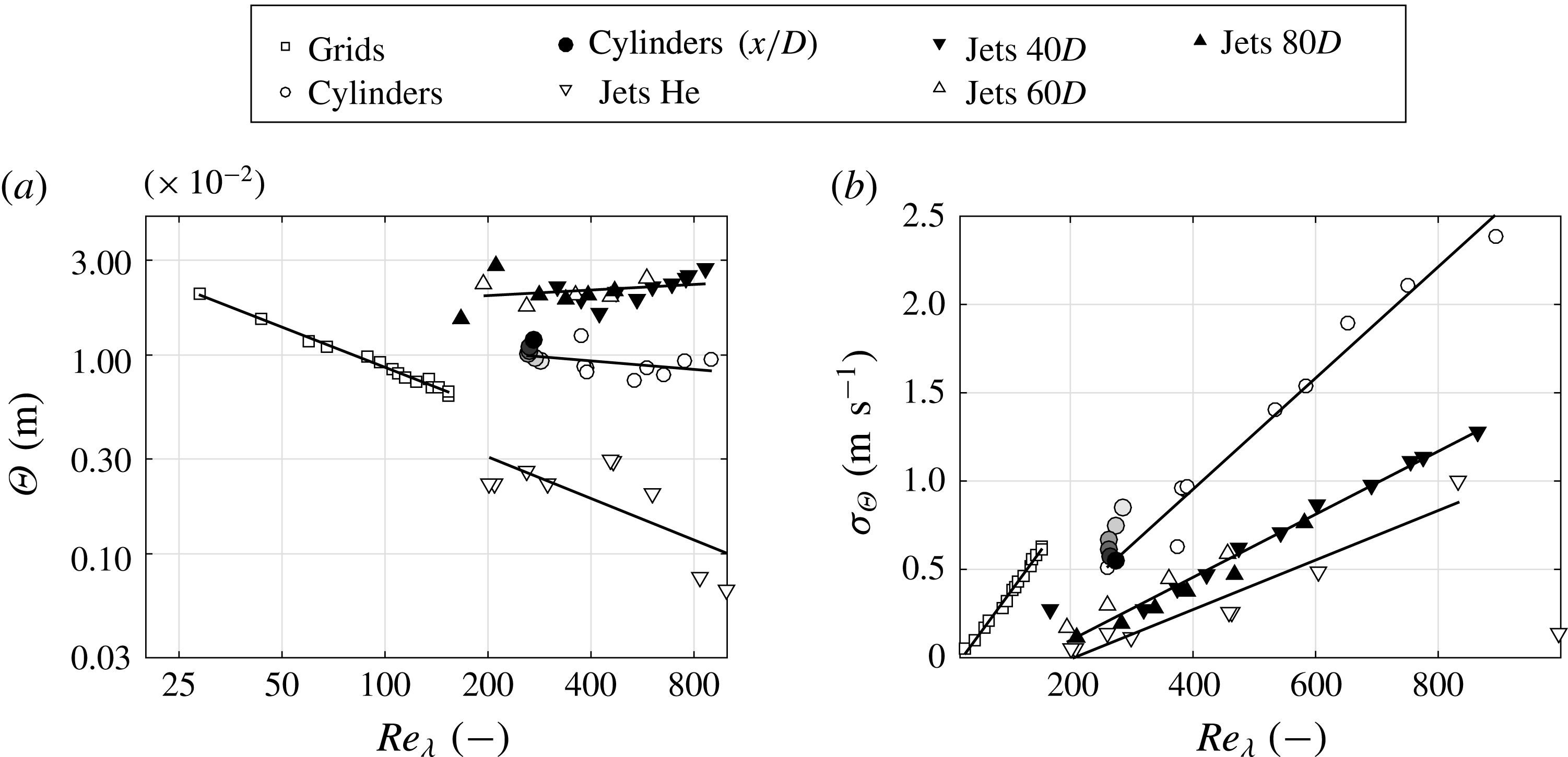
) or to be comparable in the kind of turbulence generation. Characteristic quantities of these datasets are summarised in table 1. The listed quantities are longitudinal integral length
 $L$
, Taylor microscale length
 $\unicode[STIX]{x1D706}$
, a newly defined Kolmogorov length scale
 $\unicode[STIX]{x1D6E9}$
, standard deviation of the velocity
 $\unicode[STIX]{x1D70E}_{v}$
and a newly defined standard deviation
 $\unicode[STIX]{x1D70E}_{\unicode[STIX]{x1D6E9}}$
for normalisation.
Exemplary datasets and their characteristics.

To estimate
 $\unicode[STIX]{x1D706}$
, the procedure proposed by Aronson & Löfdahl (Reference Aronson and Löfdahl1993) is used, in good agreement with the findings in Renner et al. (Reference Renner, Peinke and Friedrich2001) and Lück et al. (Reference Lück, Renner, Peinke and Friedrich2006). The integral length
 $L$
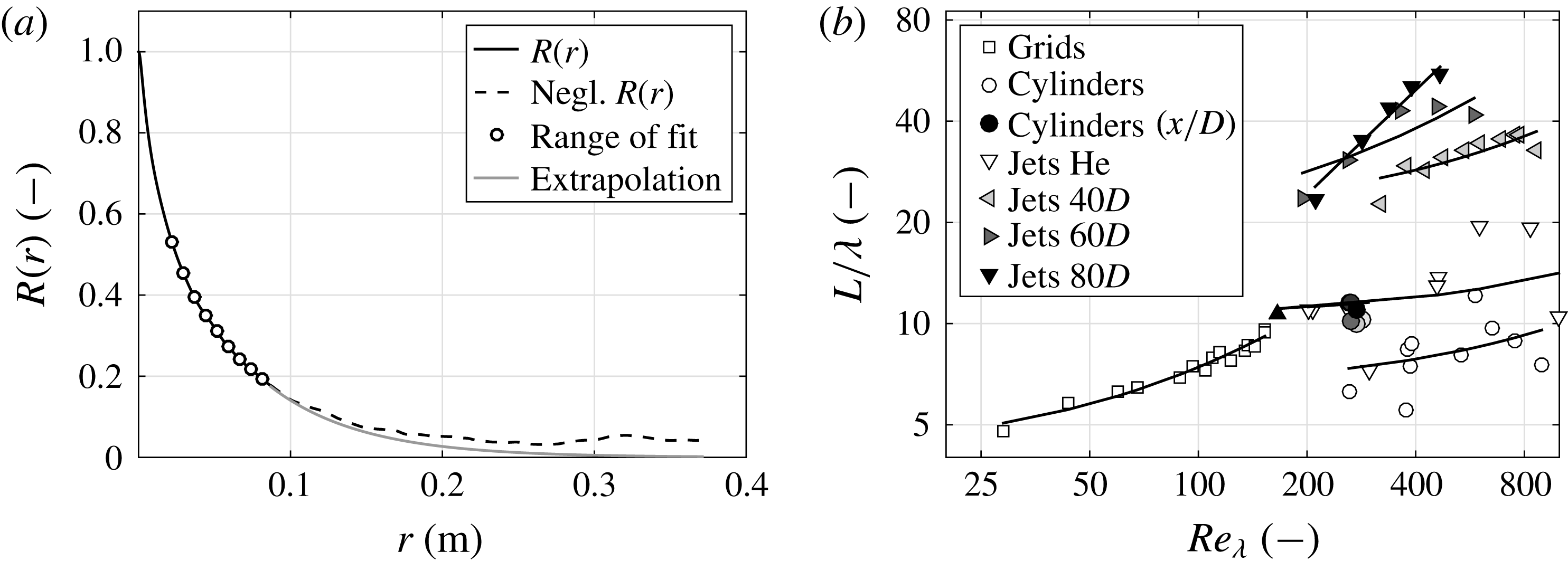
is estimated by integrating the autocorrelation function, cf. Batchelor (Reference Batchelor1953). In the case of a non-monotonic decrease of the autocorrelation function (until first zero crossing), the autocorrelation function is extrapolated by an exponential function, cf. Reinke et al. (Reference Reinke, Fuchs, Hölling and Peinke2014). More information regarding this procedure can be found in § A.1. The results for
 $L$
match with findings in Renner et al. (Reference Renner, Peinke and Friedrich2001) and Lück et al. (Reference Lück, Renner, Peinke and Friedrich2006). It should be noted also that the ratio
 $L/\unicode[STIX]{x1D706}$
as a function of
 $Re_{\unicode[STIX]{x1D706}}$
is shown in § A.1, which demonstrates the consistency of the datasets used. The terms
 $\unicode[STIX]{x1D6E9}$
and
 $\unicode[STIX]{x1D70E}_{\unicode[STIX]{x1D6E9}}$
are defined in § 3.
3 Methods of analysis
This section discusses the methods we use to analyse our data. First, the classical method based on structure functions is briefly summarised, before we discuss in some more detail the method used to achieve a multiscale analysis by means of stochastic processes. In particular, the procedure to obtain a best estimate for a cascade Fokker–Planck equation from the data is discussed. Finally, we show how the estimated cascade equation can be used to determine the entropies for which the integral fluctuation theorem is a rigorous law.
3.1 Classical analysis
First, datasets of velocity time series are transferred to spatial velocity series by use of Taylor’s hypothesis,
 $$\begin{eqnarray}v(\text{d}x)\approx v(-\langle v(t)\rangle \,\text{d}t),\end{eqnarray}$$
where
 $v$
denotes the velocity component in the main flow direction,
 $x$
is the spatial component in the main flow direction,
 $t$
is time and
 $\langle \cdots \rangle$
denotes the expectation value. The minus sign in (3.1) aligns the orientation of the
 $x$
-axis with the flow direction. Taylor’s hypothesis of frozen turbulence is commonly known as a good approximation for small velocity fluctuations
 $v^{\prime }/\langle v\rangle \ll 1$
, cf. Taylor (Reference Taylor1938), or small turbulence intensities, i.e. smaller than 10 %–20 %, cf. Murzyn & Bélorgey (Reference Murzyn and Bélorgey2005). This limit is fulfilled for almost all datasets. Further discussion of the validity can be found, e.g., in Lin (Reference Lin1953), Lumley (Reference Lumley1965), Pinton & Labbé (Reference Pinton and Labbé1994), Tong & Warhaft (Reference Tong and Warhaft1995) and Gledzer (Reference Gledzer1997).
A standard quantity to analyse the scaling of turbulence is the velocity increment
 $$\begin{eqnarray}u_{r}^{\ast }:=v(x+r)-v(x),\end{eqnarray}$$
which is the difference of velocities at two points separated by the distance
 $r$
; therefore, its statistics is referred to as one-scale statistics or respectively two-point statistics on scale
 $r$
. A common quantity for the analysis of turbulence is the so-called structure function of order
 $\unicode[STIX]{x1D705}$
,
 $$\begin{eqnarray}S^{\unicode[STIX]{x1D705}}(r)=\langle (u_{r}^{\ast })^{\unicode[STIX]{x1D705}}\rangle .\end{eqnarray}$$
Within the inertial range, it is commonly proposed that for homogeneous isotropic turbulence, structure functions scale according to a power law (Kolmogorov Reference Kolmogorov1941),
 $$\begin{eqnarray}S^{\unicode[STIX]{x1D705}}(r)\propto r^{\unicode[STIX]{x1D709}_{\unicode[STIX]{x1D705}}}.\end{eqnarray}$$
Kolmogorov (Reference Kolmogorov1962) proposed a refined approach for the structure function exponent (K62),
 $$\begin{eqnarray}\unicode[STIX]{x1D709}_{\unicode[STIX]{x1D705}}=\frac{\unicode[STIX]{x1D705}}{3}-\frac{\unicode[STIX]{x1D707}}{18}\unicode[STIX]{x1D705}(\unicode[STIX]{x1D705}-3),\end{eqnarray}$$
with the experimentally measured intermittency factor
 $\unicode[STIX]{x1D707}\approx 0.26$
, e.g. Arneodo et al. (Reference Arneodo, Baudet, Belin, Benzi, Castaing, Chabaud, Chavarria, Ciliberto, Camussi, Chillá, Dubrulle, Gagne, Hebral, Herweijer, Marchand, Maurer, Muzy, Naert, Noullez, Peinke, Roux, Tabeling, van de Water and Willaime1996). While Kolmogorov proposed that the scaling exponents
 $\unicode[STIX]{x1D709}_{\unicode[STIX]{x1D705}}$
are constant in
 $r$
, a local scaling exponent
 $\unicode[STIX]{x1D709}_{\unicode[STIX]{x1D705}}(r)$
can be calculated from experimental data by the log–log derivative of structure functions. Here, the central difference quotient is used,
 $$\begin{eqnarray}\unicode[STIX]{x1D709}_{\unicode[STIX]{x1D705}}(r)=\lim _{\unicode[STIX]{x1D6FF}r\rightarrow 0}\frac{\ln (\langle (u_{r+\unicode[STIX]{x1D6FF}r}^{\ast })^{\unicode[STIX]{x1D705}}\rangle )-\ln (\langle (u_{r-\unicode[STIX]{x1D6FF}r}^{\ast })^{\unicode[STIX]{x1D705}}\rangle )}{\ln (r+\unicode[STIX]{x1D6FF}r)-\ln (r-\unicode[STIX]{x1D6FF}r)}.\end{eqnarray}$$
Experimental results (as shown below) show that the range of constant scaling is rather small or even infinitesimal in the case of finite Taylor based Reynolds numbers (
 $Re_{\unicode[STIX]{x1D706}}\leqslant 1000$
). This motivates us to define a specific scale
 $\unicode[STIX]{x1D6E9}$
at
 $\unicode[STIX]{x1D709}_{2}(\unicode[STIX]{x1D6E9})=0.696$
, where the scaling proposed by Kolmogorov is located. Correspondingly, a standard deviation
 $\unicode[STIX]{x1D70E}_{\unicode[STIX]{x1D6E9}}=\sqrt{\langle (u_{r=\unicode[STIX]{x1D6E9}}^{\ast })^{2}\rangle }$
is defined. Here, we call
 $\unicode[STIX]{x1D6E9}$
the Kolmogorov length scale (of second order).
For the comparison of the statistics of
 $u_{r}^{\ast }$
, it is necessary that velocity increments are normalised in a proper way. On the one hand, we follow the method proposed by Renner et al. (Reference Renner, Peinke and Friedrich2001), where a norm based on a second-order structure function is used, and on the other hand, we are inspired by the work of Mydlarski & Warhaft (Reference Mydlarski and Warhaft1996), where features of the inertial range are investigated. To account for both, we select
 $\unicode[STIX]{x1D70E}_{\unicode[STIX]{x1D6E9}}$
for the purpose of normalisation,
 $$\begin{eqnarray}u_{r}:=\frac{u_{r}^{\ast }}{\unicode[STIX]{x1D70E}_{\unicode[STIX]{x1D6E9}}}.\end{eqnarray}$$
The benefit of this normalisation becomes more clear below and it should be noted that this normalisation can be applied without loss of generality in scaling features. This fact can easily be shown, for instance with (3.3) and (3.4), where a multiplication with an arbitrary factor does not change the scaling exponent.
3.2 Joint multiscale analysis
Structure functions can be expressed in terms of unconditional PDFs
 $p(u_{r})$
,
 $$\begin{eqnarray}S^{\unicode[STIX]{x1D705}}(r)=\displaystyle \int _{-\infty }^{+\infty }u_{r}^{\unicode[STIX]{x1D705}}p(u_{r})\,\text{d}u_{r}.\end{eqnarray}$$
Thus, the information given by all structure functions is equivalent to the information of
 $p(u_{r})$
at
 $r$
, cf. Frisch (Reference Frisch2001). Approaches using (3.8) consider the statistical features for each scale separately. As the turbulent cascade is a chain of events on different scales, a more appropriate approach sets the statistics of scales in relation to each other. An
 $N$
-scale joint PDF
 $p(u_{r};u_{r+\unicode[STIX]{x1D6E5}};u_{r+2\unicode[STIX]{x1D6E5}};\ldots ;u_{r+N\unicode[STIX]{x1D6E5}})$
captures the entire multiscale characteristics of the turbulent cascade including its relations over different scales, cf. Friedrich & Peinke (Reference Friedrich and Peinke1997a
).
Earlier studies show that both the turbulent cascade process and its increment series have the Markov property, e.g. Friedrich & Peinke (Reference Friedrich and Peinke1997a ), Renner et al. (Reference Renner, Peinke and Friedrich2001, Reference Renner, Peinke, Friedrich, Chanal and Chabaud2002b ), Tutkun & Mydlarski (Reference Tutkun and Mydlarski2004), Lück et al. (Reference Lück, Renner, Peinke and Friedrich2006). Thus, general joint PDFs can be expressed by conditional PDFs,
 $$\begin{eqnarray}\displaystyle p(u_{r};u_{r+\unicode[STIX]{x1D6E5}};\ldots ;u_{r+N\unicode[STIX]{x1D6E5}})=p(u_{r}|u_{r+\unicode[STIX]{x1D6E5}})p(u_{r+\unicode[STIX]{x1D6E5}}|u_{r+2\unicode[STIX]{x1D6E5}})\times \cdots & & \displaystyle \nonumber\\ \displaystyle \times \,p(u_{r+(N-1)\unicode[STIX]{x1D6E5}}|u_{r+N\unicode[STIX]{x1D6E5}})p(u_{r+N\unicode[STIX]{x1D6E5}}). & & \displaystyle\end{eqnarray}$$
Motivated by the cascade picture, our notation here implies that an increment
 $u_{r}$
is conditioned on an increment on a larger scale
 $u_{r+\unicode[STIX]{x1D6E5}}$
.
The Markov property is commonly only valid for finite step sizes, in particular when the deterministic microscopic or smallest-scale dynamics is coarse-grained to a stochastic dynamics, cf. Einstein (Reference Einstein1905). In the case of the turbulent cascade, it is valid for
 $\unicode[STIX]{x1D6E5}\geqslant l_{EM}$
, where
 $l_{EM}$
is the Einstein–Markov coherence length and it is
 $l_{EM}\propto \unicode[STIX]{x1D706}$
, cf. Lück et al. (Reference Lück, Renner, Peinke and Friedrich2006), Stresing et al. (Reference Stresing, Kleinhans, Friedrich and Peinke2012). Unless stated otherwise, we take the step width in the cascade as
 $\unicode[STIX]{x1D6E5}=l_{EM}=2\unicode[STIX]{x1D706}$
. Details of the determination of the Einstein–Markov coherence length are given in § A.2. Thus, the stochastic process at scale
 $r$
is determined by the conditional PDF
 $p(u_{r}|u_{r+l_{EM}})$
, and the entire cascade with its interscale relations can be described by
 $p(u_{r}|u_{r+l_{EM}})$
as a function of
 $r$
.
Starting from an initial distribution, e.g. at the integral length scale
 $p(u_{L})$
or any other starting scale
 $r^{\prime }$
, the evolution of
 $p(u_{r}|u_{L})$
can be described by the Fokker–Planck equation (also known as the Kolmogorov equation), cf. Friedrich & Peinke (Reference Friedrich and Peinke1997a
,Reference Friedrich and Peinke
b
), Renner et al. (Reference Renner, Peinke and Friedrich2001),
 $$\begin{eqnarray}\displaystyle -\frac{\unicode[STIX]{x2202}}{\unicode[STIX]{x2202}r}p(u_{r}|u_{r^{\prime }}) & = & \displaystyle -\frac{\unicode[STIX]{x2202}}{\unicode[STIX]{x2202}u_{r}}[D^{(1)}(u_{r})p(u_{r}|u_{r^{\prime }})]\nonumber\\ \displaystyle & & \displaystyle +\,\frac{\unicode[STIX]{x2202}^{2}}{\unicode[STIX]{x2202}u_{r}^{2}}[D^{(2)}(u_{r})p(u_{r}|u_{r^{\prime }})].\end{eqnarray}$$
Thereby, any
 $p(u_{r}|u_{r^{\prime }})$
with
 $r<r^{\prime }$
can be obtained. The functions
 $D^{(1)}(u_{r})$
and
 $D^{(2)}(u_{r})$
govern the Fokker–Planck equation and are known as drift and diffusion functions, or, more generally, first and second Kramers–Moyal coefficients. The Fokker–Planck equation is a truncated Kramers–Moyal expansion, cf. Risken (Reference Risken1984), where only the first two terms are considered. Due to the fact that the first two terms of the Kramers–Moyal expansion strongly dominate the expansion, cf. Renner et al. (Reference Renner, Peinke and Friedrich2001), Tutkun & Mydlarski (Reference Tutkun and Mydlarski2004), the description of the evolution of the conditional PDFs in scale by the Fokker–Planck equation is justified. This dominance can be related to Pawula’s theorem, which further corroborates the use of the Fokker–Planck equation, cf. Risken (Reference Risken1984).
The Fokker–Planck approach can be related to structure functions by partial integration of (3.10), e.g. Friedrich, Peinke & Naert (Reference Friedrich, Peinke and Naert1997), Renner et al. (Reference Renner, Peinke and Friedrich2001),
 $$\begin{eqnarray}\displaystyle -r\frac{\unicode[STIX]{x2202}}{\unicode[STIX]{x2202}r}S^{\unicode[STIX]{x1D705}}(r)=r\unicode[STIX]{x1D705}\langle u_{r}^{(\unicode[STIX]{x1D705}-1)}D^{(1)}(u_{r})\rangle +r\unicode[STIX]{x1D705}(\unicode[STIX]{x1D705}-1)\langle u_{r}^{(\unicode[STIX]{x1D705}-2)}D^{(2)}(u_{r})\rangle . & & \displaystyle\end{eqnarray}$$
It is easily seen that this set of equations for
 $S^{\unicode[STIX]{x1D705}}$
becomes unclosed if the drift and diffusion functions have higher-order contributions in
 $u_{r}$
(
 $D^{(1)}$
higher than linear,
 $D^{(2)}$
higher than quadratic).
Besides the Fokker–Planck equation, the two coefficients
 $D^{(1)}(u_{r})$
and
 $D^{(2)}(u_{r})$
define the equivalent Langevin equation (cf. Risken Reference Risken1984). The Langevin equation describes the evolution of increments
 $u_{r}$
in
 $r$
as trajectories
 $u(\cdot )$
. The trajectory level illustrates our novel way of investigating turbulence by considering cascade trajectories of increments
 $u_{L}\rightarrow u_{r}$
.
3.3 Estimation of Kramers–Moyal coefficients
Next, technical aspects are discussed on how to estimate the best Fokker–Planck equation. Kramers–Moyal coefficients can be estimated from given data by conditional moments,
 $$\begin{eqnarray}\displaystyle M^{(\unicode[STIX]{x1D705})}(u_{r^{\prime }},\unicode[STIX]{x1D6FF}) & = & \displaystyle \displaystyle \int _{-\infty }^{+\infty }(\tilde{u_{r}}-u_{r^{\prime }})^{\unicode[STIX]{x1D705}}p(\tilde{u_{r}}|u_{r^{\prime }})\,\text{d}\tilde{u_{r}},\end{eqnarray}$$
 $$\begin{eqnarray}\displaystyle & = & \displaystyle \langle [\tilde{u_{r}}-u_{r^{\prime }}]^{\unicode[STIX]{x1D705}}\rangle |_{u_{r^{\prime }}},\end{eqnarray}$$
 $$\begin{eqnarray}\displaystyle D^{(\unicode[STIX]{x1D705})}(u_{r^{\prime }}) & = & \displaystyle \lim _{\unicode[STIX]{x1D6FF}\rightarrow 0}\frac{1}{\unicode[STIX]{x1D705}!\unicode[STIX]{x1D6FF}}~M^{(\unicode[STIX]{x1D705})}(u_{r^{\prime }},\unicode[STIX]{x1D6FF}),\end{eqnarray}$$
where
 $\unicode[STIX]{x1D705}$
is the order of the coefficient, cf. Risken (Reference Risken1984), and
 $\unicode[STIX]{x1D6FF}=r^{\prime }-r$
. A common method to estimate
 $\lim _{\unicode[STIX]{x1D6FF}\rightarrow 0}$
in (3.14) is an extrapolation. The evolution of moments
 $M^{(\unicode[STIX]{x1D705})}(u_{r},\unicode[STIX]{x1D6FF})$
between
 $\unicode[STIX]{x1D6FF}=l_{EM}$
and
 $\unicode[STIX]{x1D6FF}=2l_{EM}$
is linearly extrapolated to
 $\unicode[STIX]{x1D6FF}=0$
and the intersection with the ordinate axis estimates the limit. Kramers–Moyal coefficients deduced by this approach lead to a rather imprecise description of the turbulent cascade. Further improvements are possible with the use of higher-order corrections, see Risken (Reference Risken1984) and discussions of this issue in Renner (Reference Renner2002), Gottschall & Peinke (Reference Gottschall and Peinke2008) and Honisch & Friedrich (Reference Honisch and Friedrich2011). Nevertheless, the limit approximation leads to uncertainties and still leaves room for improvements in their absolute values, whereas the functional forms of Kramers–Moyal coefficients are commonly well estimated.
To determine the Kramers–Moyal coefficients, an optimisation procedure is used to minimise possible uncertainties, which was proposed in Nawroth et al. (Reference Nawroth, Peinke, Kleinhans and Friedrich2007) and Kleinhans et al. (Reference Kleinhans, Friedrich, Nawroth and Peinke2005). Four steps are necessary for this optimisation: (i) parametrisation of Kramers–Moyal coefficients, (ii) calculation of
 $p(u_{r};u_{r+l_{EM}})$
, (iii) estimation of the difference between the calculated distribution
 $p(u_{r};u_{r+l_{EM}})$
and the measured joint PDF, and (iv) an iterative optimisation procedure that finds best fitting Kramers–Moyal coefficients, ensuring a minimal distance between the distributions.
We discuss the four steps in detail.
Step (i) A common parametrisation (
 $d_{ij}$
) of the Kramers–Moyal coefficients is a linear function for
 $D^{(1)}$
and a parabolic function for
 $D^{(2)}$
,
 $$\begin{eqnarray}\displaystyle & \displaystyle D^{(1)}(u_{r})=d_{11}(r)u_{r}, & \displaystyle\end{eqnarray}$$
 $$\begin{eqnarray}\displaystyle & \displaystyle D^{(2)}(u_{r})=d_{22}(r)u_{r}^{2}+d_{20}(r). & \displaystyle\end{eqnarray}$$
As we will see later, these functions conform well with the shape of
 $D^{(1)}$
and
 $D^{(2)}$
(also denoted as
 $D^{(1,2)}$
) constructed from the measurement data.
Step (ii) A calculation of
 $p(u_{r}|u_{r+l_{EM}})$
is made by use of the short-time propagator (Risken Reference Risken1984; Renner et al.
Reference Renner, Peinke and Friedrich2001),
 $$\begin{eqnarray}\displaystyle p_{STP}(u_{r}|u_{r+l_{EM}}) & {\approx} & \displaystyle \frac{1}{\sqrt{4\unicode[STIX]{x1D70B}\;D^{(2)}(u_{r+l_{EM}})\;l_{EM}}}\nonumber\\ \displaystyle & & \displaystyle \times \exp \left(-\frac{[u_{r}-u_{r+l_{EM}}-D^{(1)}(u_{r+l_{EM}})l_{EM}]^{2}}{4D^{(2)}(u_{r+l_{EM}})l_{EM}}\right).\end{eqnarray}$$
This particular functional form of (3.17) is reached by implementing the scale step in units of the Einstein–Markov coherence length
 $l_{EM}$
, which has the advantage that the short-time propagator only depends on
 $D^{(1,2)}$
. (The proper size of a scale step in (3.17) is investigated by use of the Chapman–Kolmogorov equation, cf. Risken (Reference Risken1984). The specified step size
 $l_{EM}$
leads to consistent results; smaller steps than
 $l_{EM}$
do not significantly improve the results.)
Since the experimentally found conditional PDFs
 $p_{exp}(u_{r}|u_{r+l_{EM}})$
become noisy at large values of
 $u_{r}$
and
 $u_{r+l_{EM}}$
, it is better to use the joint PDFs for the optimisation procedure. Therefore, conditional PDFs
 $p_{STP}(u_{r}|u_{r+l_{EM}})$
from (3.17) are converted by Bayes’ theorem to joint PDFs
 $p_{STP}(u_{r};u_{r+l_{EM}})$
.
Step (iii) Next, we set the numerical calculated joint PDF
 $p_{STP}$
in comparison with the measured reference
 $p_{exp}$
by use of a weighted mean square error function in logarithmic space, cf. Feller (Reference Feller1968) (analogous to Kullback–Leibler entropy),
 $$\begin{eqnarray}\unicode[STIX]{x1D716}(p_{STP},p_{exp})=\frac{\displaystyle \int _{-\infty }^{+\infty }\displaystyle \int _{-\infty }^{+\infty }(p_{STP}+p_{exp})(\ln (p_{STP})-\ln (p_{exp}))^{2}\,\text{d}u_{r}^{2}}{\displaystyle \int _{-\infty }^{+\infty }\displaystyle \int _{-\infty }^{+\infty }(p_{STP}+p_{exp})(\ln ^{2}(p_{STP})+\ln ^{2}(p_{exp}))\,\text{d}u_{r}^{2}},\end{eqnarray}$$
with
 $\ln$
as the natural logarithm. The term
 $\unicode[STIX]{x1D716}$
is taken as a logarithmic measure for the distance between the distributions.
Step (iv) The logarithmic distance
 $\unicode[STIX]{x1D716}$
is taken as a cost function for an optimisation procedure. The optimisation procedure systematically changes
 $D^{(1,2)}$
until
 $\unicode[STIX]{x1D716}$
is minimised. The optimisation procedure is a second-order method based on a Hessian matrix. We used for this optimisation the function fmincon implemented in MATLAB® R2012a. The constraints were set in a physically and mathematically meaningful way,
 $-\infty \leqslant d_{11}\leqslant 0$
,
 $0\leqslant d_{22}\leqslant \infty$
and
 $0<\unicode[STIX]{x1D6FF}_{d}\leqslant d_{20}\leqslant \infty$
; here,
 $\unicode[STIX]{x1D6FF}_{d}=10^{-3}$
.
3.4 Integral fluctuation theorem
Next, we present the IFT and its thermodynamic origin as a new physical law for the turbulent cascade and, furthermore, as an independent measure to show the validity of the Markov description of the cascade. In addition, the functional form of the estimated functions
 $D^{(1,2)}$
is disclosed and assessed by the IFT.
The Kramers–Moyal coefficients describe the turbulent system and its increment trajectories from an initial state given by
 $p(u_{L},L)$
to a final state
 $p(u_{\unicode[STIX]{x1D706}},\unicode[STIX]{x1D706})$
. The corresponding stochastic process that defines the evolution in scale of an initial increment
 $u_{L}$
drawn from
 $p(u_{L},L)$
down to the final increment
 $u_{\unicode[STIX]{x1D706}}$
can be interpreted as an analogue of a non-equilibrium thermodynamic process. Most importantly, drawing the analogy to non-equilibrium thermodynamics entails the notion of irreversible entropy production for a turbulent cascade, with useful implications. Now, we make a short digression into non-equilibrium thermodynamics to explain the background in more detail.
In non-equilibrium thermodynamics, external forces generate a deterministic drift
 $D^{(1)}$
, and the thermal energy
 $k_{B}T$
defines the diffusion function
 $D^{(2)}$
. The drift and the diffusion function are the two ingredients to set up the Fokker–Planck equation or, equivalently, the Langevin equation of non-equilibrium thermodynamic processes, cf. Lemons (Reference Lemons1997), Sekimoto (Reference Sekimoto1998). For a turbulent cascade, the linear drift
 $D^{(1)}(u_{r})$
in (3.15) accounts for the tendency of turbulent structures to split into smaller structures, invoked by the nonlinearity of the Navier–Stokes equation.
Drawing the analogy further, just as the thermal movement of the particles of an embedding medium is a source of fluctuations for a system of interest, we interpret
 $u_{r}^{2}$
as an energetic term being a source of velocity fluctuations throughout the turbulent cascade
 $u_{r}$
itself. The functional form of the fluctuation describing the coefficient
 $D^{(2)}(u_{r})$
in (3.16) hence suggests that the
 $r$
dependence of the
 $d_{22}(r)$
term constitutes the influence of turbulent energy on small-scale intermittency. This interpretation receives support from the role of the energy transfer rate on the cascade, studied by Gagne, Marchand & Castaing (Reference Gagne, Marchand and Castaing1994), Naert, Friedrich & Peinke (Reference Naert, Friedrich and Peinke1997) and Renner, Peinke & Friedrich (Reference Renner, Peinke and Friedrich2002
a
). On fixing the transferred energy
 $\unicode[STIX]{x1D700}$
to a constant value or, equivalently, looking only at cascade trajectories with constant
 $\unicode[STIX]{x1D700}$
, no intermittency is observed and
 $p(u_{r}|\unicode[STIX]{x1D700})$
becomes Gaussian, i.e.
 $d_{22}(r)$
vanishes. In addition to turbulent energy as a source of fluctuations, the coefficient
 $d_{20}(r)$
procures background fluctuations independent of
 $u_{r}$
. We come back to this picture of the turbulent cascade when we discuss our results in §§ 4.3 and 4.4. For more details on the Markov picture of the cascade process, we refer the reader to Nickelsen (Reference Nickelsen2017).
From the energy balance of the thermodynamic Langevin equation, there follows an expression for the heat exchange with the medium along a single trajectory of the system, cf. Sekimoto (Reference Sekimoto1998). The heat exchange is associated with an entropy production in the medium,
 $S_{m}$
, and the change in Gibbs entropy,
 $\unicode[STIX]{x0394}s$
, which is associated with the change of system entropy. Thus, the total entropy production can be defined as
 $\unicode[STIX]{x0394}S=S_{m}+\unicode[STIX]{x0394}s$
, cf. Seifert (Reference Seifert2005).
As it is the entropy production of an isolated system,
 $\unicode[STIX]{x0394}S$
must satisfy the second law of thermodynamics,
 $\unicode[STIX]{x0394}S\geqslant 0$
. However, single fluctuations with a tendency against the average behaviour give rise to entropy consumption,
 $\unicode[STIX]{x0394}S<0$
. Therefore, it is important to remember that the second law addresses the macroscopic entropy production, which means that on average the total entropy production is non-negative,
 $\langle \unicode[STIX]{x0394}S\rangle \geqslant 0$
. Fluctuating entropy productions are central in the arising field of stochastic thermodynamics, of which one result is the so-called fluctuation theorems. These theorems express the balance between entropy production and entropy consumption by tightening the second law to an equality, cf. Seifert (Reference Seifert2012). Here, we are concerned with the IFT for the total entropy production (Seifert Reference Seifert2005),
 $$\begin{eqnarray}\langle \text{e}^{-\unicode[STIX]{x0394}S}\rangle =1.\end{eqnarray}$$
In order to amount to the average of
 $1$
, it is evident that the IFT assigns an exponential weight to the rare entropy consuming fluctuations that contribute with values much larger than
 $1$
to the average, in opposition to the typical entropy producing fluctuations that contribute with values between
 $0$
and
 $1$
. It is this delicate balance between production and consumption of entropy that makes the IFT so useful for the analysis of non-equilibrium systems. Typically, the IFT finds applications in small systems on the nanoscale, whereas its applicability is not evident for classical turbulent flows with scales in the range of mm and velocity fluctuations of order
 $\text{m}~\text{s}^{-1}$
.
At this point, we turn to turbulent cascades again and refer the interested reader to the comprehensive review by Seifert (Reference Seifert2012) for more details on stochastic thermodynamics. On the basis of single realisations of the cascade process, or, to be explicit, trajectories
 $u(\cdot )=\{u_{r};r=L\ldots \unicode[STIX]{x1D706}\}$
, the formal entropy production
 $S_{m}$
is given by, cf. Nickelsen & Engel (Reference Nickelsen and Engel2013),
 $$\begin{eqnarray}S_{m}[u(\cdot )]=\displaystyle \int _{L}^{\unicode[STIX]{x1D706}}\unicode[STIX]{x2202}_{r}u_{r}\frac{D^{(1)}(u_{r},r)-\unicode[STIX]{x2202}_{u}D^{(2)}(u_{r},r)}{D^{(2)}(u_{r},r)}\,\text{d}r.\end{eqnarray}$$
(Here, we deviate from the previous suppression of the argument
 $r$
to stress the explicit
 $r$
dependence of
 $D^{(1,2)}(u_{r},r)$
and
 $p(u_{r},r)$
.) The difference in Shannon entropy reads as
 $$\begin{eqnarray}\unicode[STIX]{x0394}s(u_{L},u_{\unicode[STIX]{x1D706}})=-\ln \frac{p(u_{\unicode[STIX]{x1D706}},\unicode[STIX]{x1D706})}{p(u_{L},L)}.\end{eqnarray}$$
If the drift and diffusion functions
 $D^{(1,2)}$
that define the cascade process as well as
 $p(u_{L},L)$
and
 $p(u_{\unicode[STIX]{x1D706}},\unicode[STIX]{x1D706})$
are known, the total entropy production for a single trajectory
 $u(\cdot )$
can formally be determined as the sum of the two contributions mentioned above,
 $$\begin{eqnarray}\unicode[STIX]{x0394}S[u(\cdot )]=S_{m}[u(\cdot )]+\unicode[STIX]{x0394}s(u_{L},u_{\unicode[STIX]{x1D706}}).\end{eqnarray}$$
If we suppose that
 $\{u(\cdot )\}$
are exact realisations of a cascade process defined by
 $D^{(1,2)}$
and
 $p(u_{L},L)$
, then
 $\langle \text{e}^{-\unicode[STIX]{x0394}S}\rangle$
should converge to exactly
 $1$
for an unlimited number of
 $u(\cdot )$
taken into account. In Nickelsen & Engel (Reference Nickelsen and Engel2013), it has been demonstrated for a single set of data from a free-jet experiment that the exponential average in the IFT is indeed converging very rapidly to
 $1$
. The crucial requirement for the convergence is the occurrence of rare trajectories with
 $\unicode[STIX]{x0394}S<0$
. Nickelsen & Engel (Reference Nickelsen and Engel2013) found that the trajectories with
 $\unicode[STIX]{x0394}S<0$
exhibit an increase of fluctuations when evolving from
 $L$
to
 $\unicode[STIX]{x1D706}$
, against the typical tendency of the cascade. It is, hence, the phenomenon of small-scale intermittency that is responsible for the applicability of the IFT to turbulent cascades and its convergence. However, a universal form of
 $D^{(1,2)}$
and therewith a universal form of the IFT is still missing. So is, e.g., the exponential average of the IFT deriving from the K62 model (3.5) diverging rapidly for the data of the free-jet experiment considered in Nickelsen & Engel (Reference Nickelsen and Engel2013), confirming the well-known fact that the K62 model does not reflect small-scale intermittency of real turbulent flows properly. For the discussion of other models of turbulence, see Nickelsen (Reference Nickelsen2017).
Here, we extend the investigations made in Nickelsen & Engel (Reference Nickelsen and Engel2013) substantially and for the first time employ the utility of the IFT to explore the role that large-scale structures play for small-scale turbulence. In doing so, we address three points. First of all, we show that the IFT holds for all different types of turbulent flows considered here and thus collect strong evidence that the IFT is a universal feature of turbulence. Second, the high sensitivity of the IFT regarding realistic modelling of small-scale intermittency enables us to verify our estimation of
 $D^{(1,2)}$
and to quantify the importance and significance of different functional contributions of
 $D^{(1,2)}$
. Finally, the interpretation as a non-equilibrium thermodynamic process illuminates the role of these functional contributions in terms of small-scale intermittency and universality.
To test the quality of the estimated functions
 $D^{(1,2)}$
, we extract
 $n$
trajectories
 $\{u(\cdot )\}$
from each of the measured flow fields
 $v(x)$
by applying the definition (3.2) for different values of
 $x$
. To ensure the independence of the trajectories, we take equidistant values for
 $x$
with step size
 $L$
, due to the fact that
 $L$
specifies the size of the largest coherent structures in
 $v(x)$
. For each set of trajectories,
 $\{u(\cdot )\}$
, we calculate a set of total entropy productions
 $\{\unicode[STIX]{x0394}S_{j}\}$
from (3.22) in order to employ the IFT by
 $$\begin{eqnarray}1=\langle \text{e}^{-\unicode[STIX]{x0394}S[u(\cdot )]}\rangle \simeq \frac{1}{n}\mathop{\sum }_{j=1}^{n}\text{e}^{-\unicode[STIX]{x0394}S_{j}}=:I(n).\end{eqnarray}$$
The overall implementation of the IFT is then as follows. For each of the datasets considered here, the values of
 $D^{(1,2)}$
are estimated and used to define the form of
 $S_{m}$
in (3.20),
 $p(u_{L},L)$
and
 $p(u_{\unicode[STIX]{x1D706}},\unicode[STIX]{x1D706})$
are estimated to define
 $\unicode[STIX]{x0394}s$
in (3.21), and the very data that were used for this estimation are plugged into the IFT. If the IFT is confirmed, the Markov process defined by
 $D^{(1,2)}$
and the initial condition
 $p(u_{L},L)$
correctly captures the cascade process and in particular the small-scale features of the turbulent flow. In addition to this quality check, the IFT serves as a clear-cut criterion to pin down and discuss the minimal functional form of
 $D^{(1,2)}$
that still captures the cascade process.
4 Results
In this section, we show the results obtained from all 61 datasets. The analysis of structure functions sets our data into the common picture of turbulence and checks whether the data obey a scaling law. Subsequently, we demonstrate and discuss the validity of the IFT and our parametrisation of the Kramers–Moyal coefficients, followed by a discussion of their functional form. Thereafter, results of multiscale statistics are presented and discussed in the context of universal and non-universal flow dependences of turbulence.
4.1 Two-point scaling features
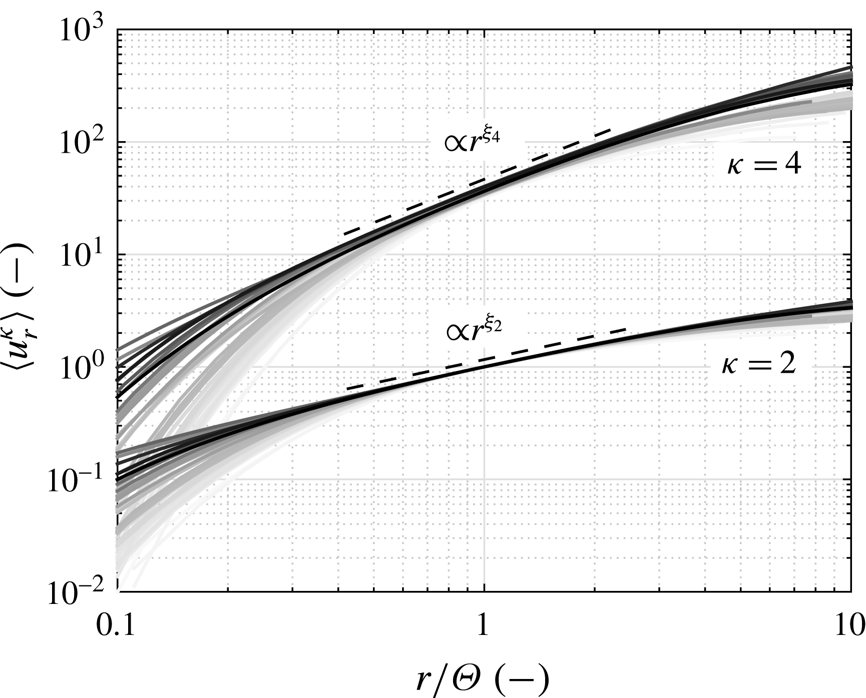
We begin with the standard analysis of our data. Figure 1 presents second- (
 $\unicode[STIX]{x1D705}=2$
) and fourth-order (
 $\unicode[STIX]{x1D705}=4$
) structure functions according to (3.3) obtained from all datasets. The lower band corresponds to second-order and the upper band to fourth-order structure functions. The greyscale of the curves indicates the Taylor–Reynolds numbers. It is clearly seen how the scaling range increases with
 $Re_{\unicode[STIX]{x1D706}}$
. The structure functions are normalised in their scale and in their values by
 $\unicode[STIX]{x1D6E9}$
and
 $\unicode[STIX]{x1D70E}_{\unicode[STIX]{x1D6E9}}$
, defined in § 3.1. The band of the fourth-order structure functions is shifted by a factor of
 $10$
along the ordinate axis for reasons of presentation. The norms
 $\unicode[STIX]{x1D6E9}$
and
 $\unicode[STIX]{x1D70E}_{\unicode[STIX]{x1D6E9}}$
are shown in § A.3 as functions of
 $Re_{\unicode[STIX]{x1D706}}$
. These norms are dimensional and show features that depend also on the flow type.
Second- (
 $\unicode[STIX]{x1D705}=2$
, lower band) and fourth- (
 $\unicode[STIX]{x1D705}=4$
, higher band) order structure functions versus the normalised scale. The whole band of the fourth-order structure functions is shifted by a factor of 10 for reasons of presentation. The greyscale used for the curves indicates the corresponding Taylor–Reynolds numbers: bright grey to black corresponds to increase of
 $Re_{\unicode[STIX]{x1D706}}$
.

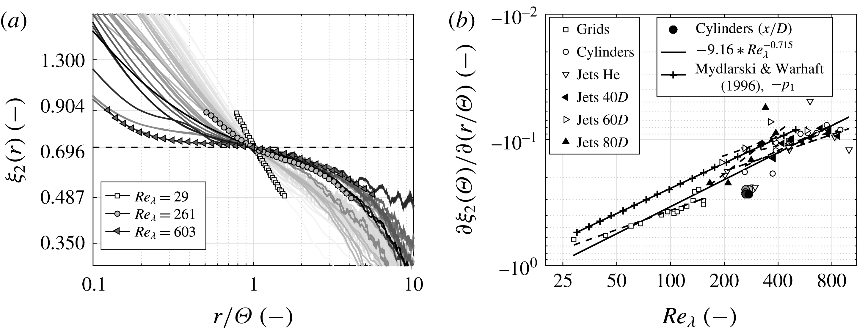
For a more precise analysis of the scaling behaviour of the structure functions, we present in figure 2(a) the local scaling exponent
 $\unicode[STIX]{x1D709}_{2}(r)$
according to (3.6). Due to our normalisation, all datasets pass through
 $\unicode[STIX]{x1D709}_{2}=0.696$
at
 $r/\unicode[STIX]{x1D6E9}=1$
. Three curves are marked by symbols to indicate that
 $\unicode[STIX]{x1D709}_{2}(r)$
changes from a linear behaviour for low
 $Re_{\unicode[STIX]{x1D706}}$
to a power-five behaviour for high
 $Re_{\unicode[STIX]{x1D706}}$
(with respect to the log–log presentation). This shows that the local scaling exponent flattens with increasing
 $Re_{\unicode[STIX]{x1D706}}$
around
 $\unicode[STIX]{x1D709}_{2}=0.696$
. Thus, instead of a stretched constant scaling range, only a tendency to usual scaling behaviour is seen, even for the highest
 $Re_{\unicode[STIX]{x1D706}}$
datasets. (By usual scaling we refer to the case where no functional deviation from a scaling law is present, i.e.
 $\unicode[STIX]{x1D709}_{\unicode[STIX]{x1D705}}(r)$
is rigorously constant in
 $r$
, e.g. (3.5).)
For the third- and fourth-order structure function, similar results are shown in Sinhuber (Reference Sinhuber2015, pp. 121–122, figures 4.3 and 4.4) and Sinhuber, Bewley & Bodenschatz (Reference Sinhuber, Bewley and Bodenschatz2017), and confirm the flattening of structure functions for even higher
 $Re_{\unicode[STIX]{x1D706}}$
for grid-generated turbulence; Grauer, Homann & Jean-Francoi (Reference Grauer, Homann and Jean-Francois2012) also used a similar approach. An explanation of this non-perfect scaling behaviour of structure functions is that finite size effects play a role (Dubrulle Reference Dubrulle2000), which also supports the idea of introducing the specific scale
 $\unicode[STIX]{x1D6E9}$
defined in § 3.1.
(a) The local second-order scaling exponent
 $\unicode[STIX]{x1D709}_{2}(r)$
according to (3.6) in a double-logarithmic plot. The presentation is like that in figure 1. (b) The slope of the local second-order scaling exponent
 $\unicode[STIX]{x1D709}_{2}(r)$
at
 $r=\unicode[STIX]{x1D6E9}$
in a double-logarithmic presentation together with data from Mydlarski & Warhaft (Reference Mydlarski and Warhaft1996).

Figure 2(b) shows the slope of the local second-order scaling exponent
 $\unicode[STIX]{x1D709}_{2}(r)$
at
 $r=\unicode[STIX]{x1D6E9}$
as a function of
 $Re_{\unicode[STIX]{x1D706}}$
. This slope is obtained by fitting a polynomial of fifth order, as shown in figure 2(a). The solid line shows the trend of all datasets with the functional form of
 $$\begin{eqnarray}\frac{\unicode[STIX]{x2202}\unicode[STIX]{x1D709}_{2}(\unicode[STIX]{x1D6E9})}{\unicode[STIX]{x2202}(r/\unicode[STIX]{x1D6E9})}\approx -9.16Re_{\unicode[STIX]{x1D706}}^{-0.715}.\end{eqnarray}$$
Based on this result,
 $\unicode[STIX]{x2202}_{(r/\unicode[STIX]{x1D6E9})}\unicode[STIX]{x1D709}_{2}(\unicode[STIX]{x1D6E9})$
can be proposed as an alternative to
 $Re_{\unicode[STIX]{x1D706}}$
.
Additional data from a similar study made by Mydlarski & Warhaft (Reference Mydlarski and Warhaft1996) are added to figure 2(b). These data represent a deviation from the common energy density spectra scaling
 $E(k)\propto k^{-5/3}$
. (It should be noted that second-order structure functions and energy density spectra contain the same information and can be converted into one another by Fourier transformation.) The deviation is expressed by
 $p_{1}$
in the form of
 $E(k)\propto k^{-(5/3-p_{1})}$
. Turbulent flows and their
 $E(k)$
values were investigated up to
 $Re_{\unicode[STIX]{x1D706}}\leqslant$
500. They found that
 $p_{1}$
has the form
 $p_{1}=5.25Re_{\unicode[STIX]{x1D706}}^{-2/3}$
, which is very similar to the
 $Re_{\unicode[STIX]{x1D706}}$
dependence we found in (4.1). The prefactor differs due to the different approaches.
4.2 Estimation procedure of Kramers–Moyal coefficients
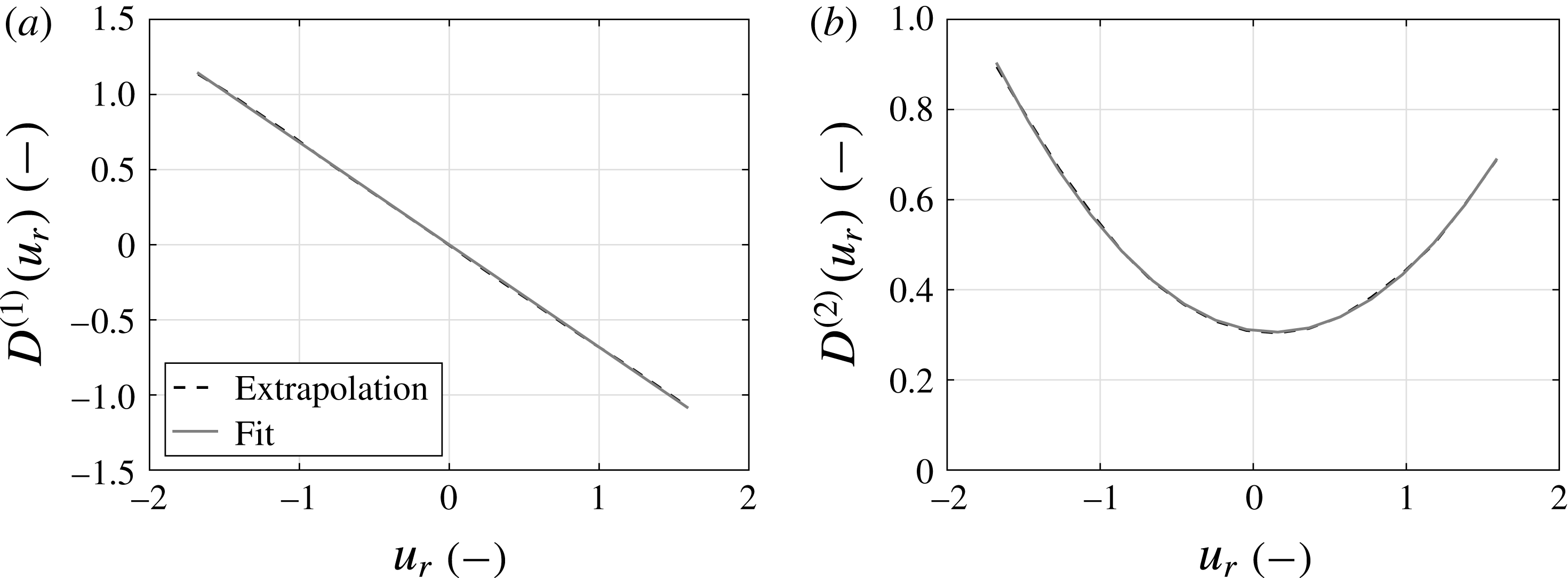
We now extend our analysis to joint multiscale statistics. The first estimation of Kramers–Moyal coefficients is based on conditional moments and their extrapolation. Figure 3 exemplarily shows
 $D^{(1)}$
and
 $D^{(2)}$
as functions of
 $u_{r}$
according to (3.14) and higher-order corrections, cf. Gottschall & Peinke (Reference Gottschall and Peinke2008). A linear and a parabolic fitting function reflect the common functional forms of
 $D^{(1,2)}$
, which are used for the subsequent optimisation. The fitting range used is indicated, namely
 $-1.5\leqslant u_{r}\leqslant 1.5$
. Here, one might argue that higher-order contributions can be seen in
 $D^{(1,2)}$
(compared with the approach in (3.15) and (3.16)). We come back to this point when we discuss the results regarding the IFT.
As a second step for the estimation of Kramers–Moyal coefficients, the optimisation procedure of § 3.3 is applied. This procedure is based on the reconstruction of PDFs according to (3.17). Figure 4 shows the quality of the reconstructed conditional PDFs by the optimised Kramers–Moyal coefficients at two different scales,
 $r=l_{EM}$
and
 $r=60l_{EM}$
. To accentuate the differences, we have chosen
 $r=60l_{EM}$
, which corresponds to a scale larger than
 $L$
. The agreement of experimental and reconstructed conditional PDFs is good.
Plots of
 $D^{(1,2)}$
versus
 $u_{r}$
, according to (3.14) and higher-order corrections, cf. Gottschall & Peinke (Reference Gottschall and Peinke2008). Linear and parabolic fitting functions illustrate their functional forms. The dataset jet 1 (table 1) is used at
 $r=1l_{EM}$
.

Contour plots showing experimental and reconstructed conditional PDFs at two different scales, (a)
 $r=l_{EM}$
and (b)
 $r=60l_{EM}$
. A dataset of subgroup (v) is used with
 $Re_{\unicode[STIX]{x1D706}}=475$
.

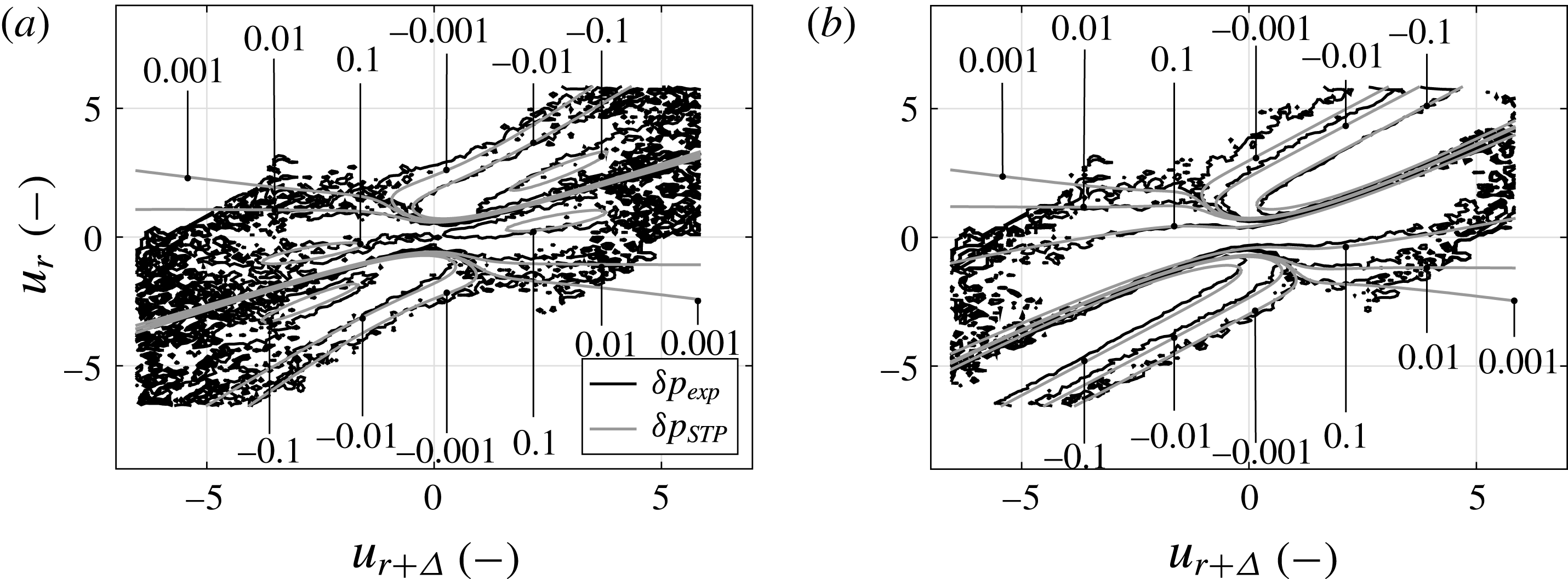
In order to further show the quality of the reconstructed conditional PDF, we analyse the change of conditional PDF along the scale, cf. (3.9) and (3.10). Figure 5 shows the cumulative change of conditional PDF, expressed as
 $$\begin{eqnarray}\displaystyle \unicode[STIX]{x1D6FF}p & = & \displaystyle [p(u_{l_{EM}}|u_{2l_{EM}})-p(u_{2l_{EM}}|u_{3l_{EM}})]\nonumber\\ \displaystyle & & \displaystyle +\,[p(u_{2l_{EM}}|u_{3l_{EM}})-p(u_{3l_{EM}}|u_{4l_{EM}})]\nonumber\\ \displaystyle & & \displaystyle +\,\cdots \nonumber\\ \displaystyle & & \displaystyle +\,[p(u_{(N-1)l_{EM}}|u_{Nl_{EM}})-p(u_{Nl_{EM}}|u_{(N+1)l_{EM}})]\end{eqnarray}$$
 $$\begin{eqnarray}\displaystyle & = & \displaystyle p(u_{l_{EM}}|u_{2l_{EM}})-p(u_{Nl_{EM}}|u_{(N+1)l_{EM}}).\end{eqnarray}$$
In figure 5,
 $\unicode[STIX]{x1D6FF}p_{exp}$
corresponds to the cumulative change of experimental data and
 $\unicode[STIX]{x1D6FF}p_{STP}$
is deduced by means of the short-time propagator (3.17) and the optimised Kramers–Moyal coefficients. Due to the scale-wise optimisation procedure, (4.2) and (4.3) are not necessarily equal for the reconstructed PDFs; thus, we use (4.2). Figure 5(a) shows
 $\unicode[STIX]{x1D6FF}p$
for
 $N=2$
(the change of the conditional PDFs at small scales) and figure 5(b) presents
 $\unicode[STIX]{x1D6FF}p$
for
 $N=60$
(the change of the conditional PDFs over a broad range of scales). We see in both figures that the distributions of
 $\unicode[STIX]{x1D6FF}p_{exp}$
and
 $\unicode[STIX]{x1D6FF}p_{STP}$
are in good agreement. Thus, the optimisation procedure works well from the smallest scale changes
 $\unicode[STIX]{x1D6FF}r=l_{EM}$
up to the cumulative change of the entire inertial range. Consequently, we assume that the description of the turbulent cascade process is properly characterised by optimised Kramers–Moyal coefficients.
It is a very strong demand on the quality of the reconstructed Kramers–Moyal coefficients to show that the conditional PDFs are well reproduced. Naturally, the commonly investigated increment PDFs
 $p(u_{r})$
and the structure functions are also reproduced well by these optimised stochastic equations. As the third-order structure function
 $S^{3}$
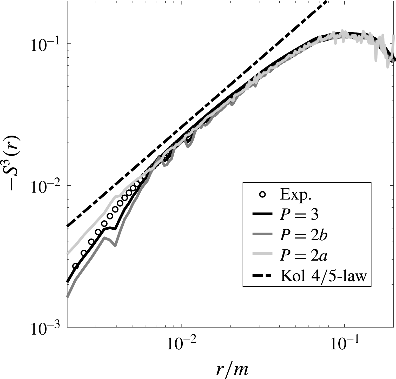
with its four-fifths law plays a key role for turbulence, we show exemplarily in figure 6 for one dataset the comparison of
 $S^{3}$
between the result of the Fokker–Planck equation and the measured one. For further discussion, see below.
The change of the conditional PDF
 $\unicode[STIX]{x1D6FF}p$
along the scale: (a)
 $\unicode[STIX]{x1D6FF}p$
for
 $N=2$
, which corresponds to small-scale change, and (b) for
 $N=60$
, which corresponds to the entire change within the inertial range. A dataset of subgroup (v) is used with
 $Re_{\unicode[STIX]{x1D706}}=475$
.

The third-order structure function
 $-S^{3}$
as a function of the scale
 $r/\unicode[STIX]{x1D6E9}$
. The results shown are obtained from the experimental data (exp) and for different functional forms of the Kramers–Moyal coefficients corresponding to the cases of table 2. In addition, the four-fifths law is shown. The dataset of subgroup vii is used with
 $Re_{\unicode[STIX]{x1D706}}=166$
.

4.3 General validity of the IFT and parametrisation of
 $D^{(1,2)}$

As a next step, we first demonstrate the validity of the IFT for our datasets and then employ the IFT to assess the quality of the optimised Kramers–Moyal coefficients and discuss their functional contributions.
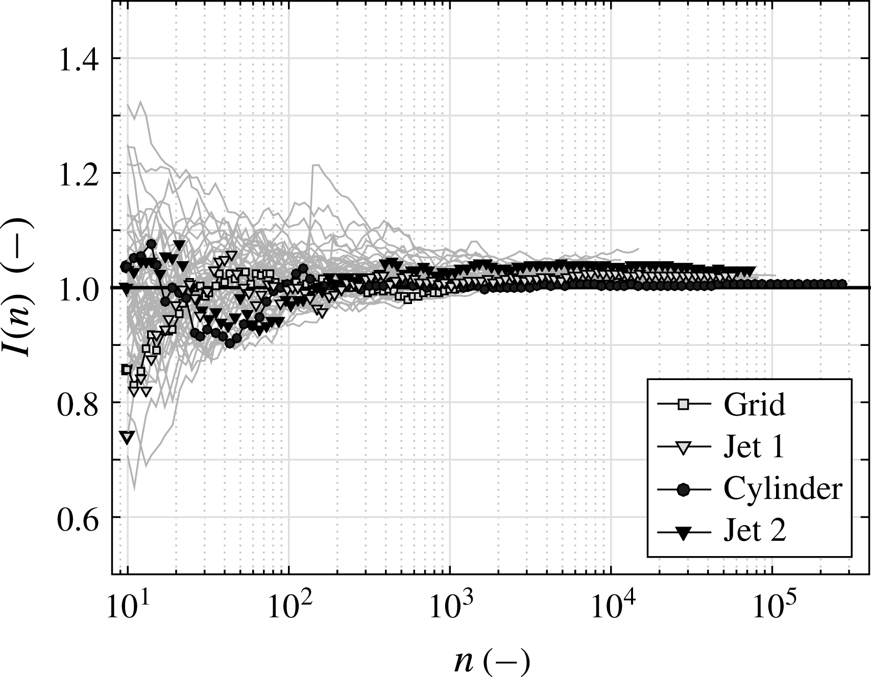
Figure 7 presents the IFT for all datasets as a function of the number
 $n$
of considered velocity increment trajectories
 $u(\cdot )$
, as stated in (3.23). Here, we used again the optimised functions
 $D^{(1,2)}$
. Due to different numbers of samples in the datasets and varying Taylor microscale as well as integral length scales, the maximal number of independent trajectories differs from dataset to dataset. The four selected datasets from table 1 are highlighted by symbols; other datasets are shown in grey. At
 $n\approx 1000$
,
 $I(n)$
has already largely converged to
 $1$
, (3.23), and only slight improvements of convergence are present at larger numbers of trajectories,
 $n>1000$
. The average of the 61 IFT values taken at
 $n=\text{maximal}$
is
 $\langle I_{max}\rangle _{datasets}\approx 1.01$
and the standard deviation of the 61
 $I_{max}$
values is
 $\unicode[STIX]{x1D70E}(I_{max})\approx 0.01$
, which we take as strong evidence that the IFT is a universal feature of turbulent cascades.


Next, we reverse the argumentation and take the IFT as a given fundamental law for the turbulent cascade. Thus, we can verify our parametrisation, and the significance of functional contributions of
 $D^{(1,2)}$
can be worked out. To test these aspects, we parametrise
 $D^{(1,2)}$
up to third order in
 $u_{r}$
(preliminary investigations with even-higher-order parametrisations do not show any improvements or other features compared with this third-order approach), i.e. with eight parameters,
 $$\begin{eqnarray}\displaystyle & \displaystyle D^{(1)}(u_{r})=d_{13}(r)u_{r}^{3}+d_{12}(r)u_{r}^{2}+d_{11}(r)u_{r}+d_{10}(r), & \displaystyle\end{eqnarray}$$
 $$\begin{eqnarray}\displaystyle & \displaystyle D^{(2)}(u_{r})=d_{23}(r)u_{r}^{3}+d_{22}(r)u_{r}^{2}+d_{21}(r)u_{r}+d_{20}(r). & \displaystyle\end{eqnarray}$$
The parameters
 $d_{ij}$
are continuous functions of
 $r$
, which is advantageous for the determination of
 $I(n)$
. To single out the important parameters among the
 $d_{ij}$
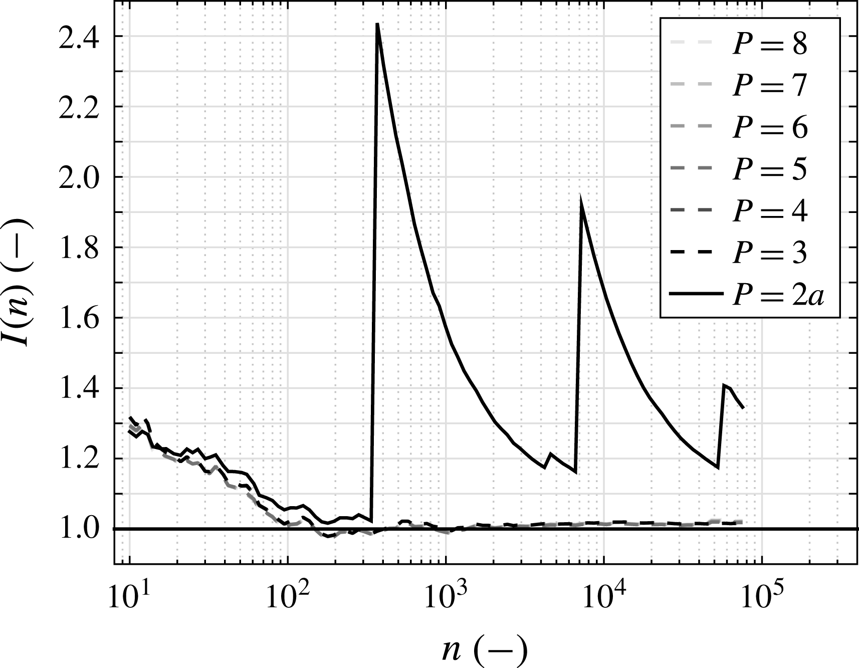
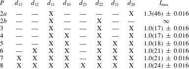
above, the number of parameters has successively been reduced from eight to two, as shown in table 2. Figure 8 presents this investigation for one exemplary dataset (subgroup (v);
 $Re_{\unicode[STIX]{x1D706}}=475$
). For each selection of parameters, the abovementioned optimisation procedure to determine
 $D^{(1,2)}$
was repeated and the IFT was tested. The resulting values
 $I_{max}$
are shown in table 2. We estimate an error of the
 $I_{max}$
by considering the convergence of the IFT (
 $1000\leqslant n\leqslant \text{maximal}$
) and its fluctuations around the saturation value
 $I_{max}$
, figure 8. In accordance with the mentioned standard deviation (
 $\unicode[STIX]{x1D70E}(I_{max})\approx 0.01$
), the estimated error is
 $0.016$
. From the results presented in table 2 and figure 8, we conclude that different functional representations of
 $D^{(1,2)}$
are possible to fulfil the IFT in good quality.


Next, we discuss the meaning of the single cases. The case
 $P=2a$
in table 2 corresponds to pure additive noise in the cascade process. This implies only Gaussian increment PDFs, i.e. no intermittency is taken into account. The value of
 $I_{max}=1.3(46)$
and the large jumps with
 $n$
evidently suggest that the IFT cannot be fulfilled with this functional ansatz, see figure 8. The jumps in the convergence are a consequence of an unbalanced weight on entropy consuming trajectories in the exponential average of the IFT. We consequently reject the case
 $P=2a$
as a functional form of
 $D^{(1,2)}$
.
The case
 $P=2b$
corresponds to pure multiplicative noise in the cascade process which includes a quadratic term in the diffusion function
 $D^{(2)}$
. It should be noted that this parametrisation corresponds to a generalisation of the scaling proposed by Kolmogorov (Reference Kolmogorov1962), see (3.5) and Friedrich & Peinke (Reference Friedrich and Peinke1997a
), Nickelsen & Engel (Reference Nickelsen and Engel2013). As the IFT diverges, this functional form is rejected as well.
For all the other choices with three and more parameters (
 $P\geqslant 3$
), we see good fulfilment of the IFT. More coefficients do not lead to a significantly better fulfilment of the IFT and its convergence. We hence conclude that the case
 $P=3$
is sufficient for a good stochastic model of the turbulent cascade that captures the features of small-scale intermittency. Higher-order terms as used in Renner et al. (Reference Renner, Peinke and Friedrich2001) and Nickelsen & Engel (Reference Nickelsen and Engel2013) seem not to be necessary. Similar stochastic models have been discussed before; see, e.g., Dubrulle (Reference Dubrulle2000) and Laval, Dubrulle & Nazarenko (Reference Laval, Dubrulle and Nazarenko2001). Starting with the Navier–Stokes equation, Laval et al. derived after certain simplifications and approximations a Langevin equation with correlated additive and multiplicative noise, which is of similar but more involved form compared with our case
 $P=3$
. The amplitude of the additive noise is related to our
 $d_{20}$
term and the amplitude of the multiplicative noise to the
 $d_{22}$
term. The conceptual difference, however, is that in Laval et al. (Reference Laval, Dubrulle and Nazarenko2001), the skewness is generated by the correlation between the two noise sources, which would imply a linear term
 $d_{21}$
(case
 $P=5$
), whereas in our model, the skewness already present at integral length scales is taken and transported down the cascade by the deterministic
 $d_{11}(r)$
term. This can also be seen in figure 6, where already the additive or multiplicative noise alone is enough to reproduce the measured skewness (cases
 $P=2a$
and
 $P=2b$
), as long as the linear drift term
 $d_{11}$
is part of the model.
To conclude, we see that the minimal functional form to fulfil the IFT is for
 $D^{(1)}$
a linear term
 $d_{10}(r)u_{r}$
, and for
 $D^{(2)}$
an additive term
 $d_{20}(r)$
as well as a quadratic term
 $d_{22}(r)u_{r}^{2}$
, which is in accordance with (3.15) and (3.16). (Renner et al. (Reference Renner, Peinke and Friedrich2002
a
) interpreted
 $d_{20}\neq 0$
and
 $d_{22}\neq 0$
as a necessary combination for turbulence and its energy cascade.) We have also recognised that
 $d_{22}$
becomes increasingly important for the fulfilment of the IFT with increasing
 $Re_{\unicode[STIX]{x1D706}}$
, indicating that small-scale intermittency becomes more dominant at higher
 $Re_{\unicode[STIX]{x1D706}}$
.
The need for the three parameters can also be discussed in the context of structure functions, see § 3.2 and (3.11). By insertion of the three parameters and a multiplication by
 $-1/S^{\unicode[STIX]{x1D705}}$
(from the left), we obtain
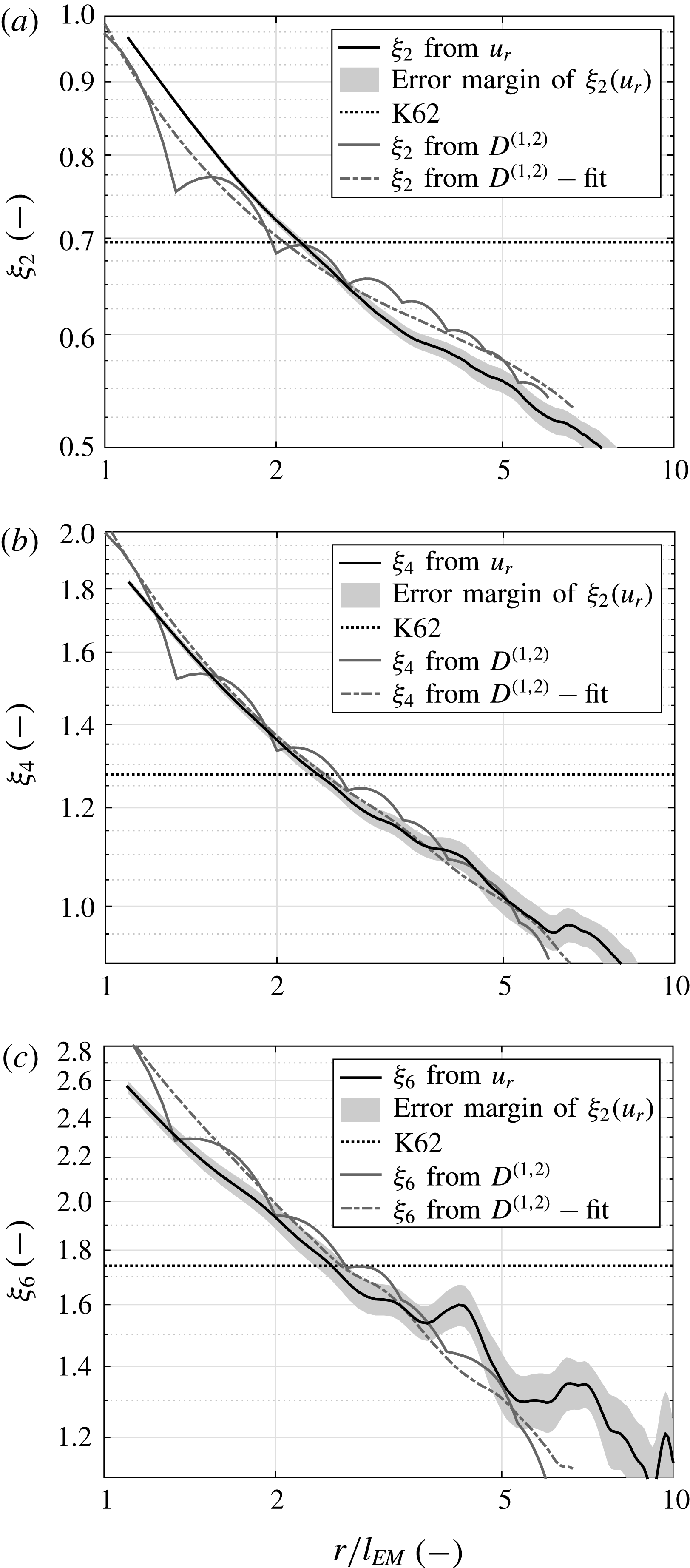
 $$\begin{eqnarray}\displaystyle \unicode[STIX]{x1D709}_{\unicode[STIX]{x1D705}}=\frac{r}{S^{\unicode[STIX]{x1D705}}}\frac{\unicode[STIX]{x2202}S^{\unicode[STIX]{x1D705}}}{\unicode[STIX]{x2202}r} & = & \displaystyle -r\unicode[STIX]{x1D705}\left(d_{11}(r)+(\unicode[STIX]{x1D705}-1)\left(d_{22}(r)+\frac{S^{(\unicode[STIX]{x1D705}-2)}(r)}{S^{\unicode[STIX]{x1D705}}(r)}d_{20}(r)\right)\right).\end{eqnarray}$$
Here, we used the substitution
 $(r/S)(\unicode[STIX]{x2202}S/\unicode[STIX]{x2202}r)=\unicode[STIX]{x2202}\ln (S)/\unicode[STIX]{x2202}\ln (r)=\unicode[STIX]{x1D709}_{\unicode[STIX]{x1D705}}(r)$
.
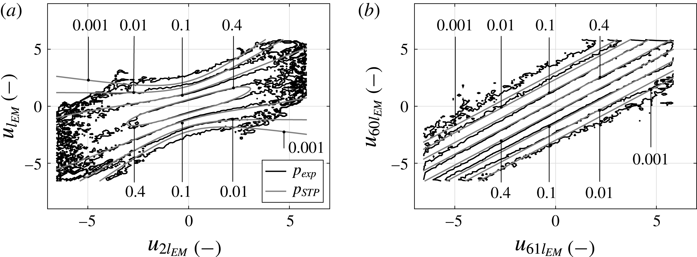
(a) The conditional PDF at
 $r=l_{EM}$
. The location of the diagonal of the conditional PDF is indicated by the function
 $d:u_{l_{EM}}=0.5u_{2l_{EM}}$
. (b) The conditional PDF at
 $r=60l_{EM}$
. The diagonal function is
 $d:u_{60l_{EM}}=u_{61l_{EM}}$
. For (a) and (b), a dataset of subgroup (v) is used with
 $Re_{\unicode[STIX]{x1D706}}=475$
.

It should be noted that the coupled set of differential equations (4.6) is closed: all structure functions can be determined successively from
 $S^{0}=1$
and
 $S^{1}=0$
. It is obvious that if more parameters were needed, (4.6) would become more complicated. In the case of negligible
 $d_{20}$
, (4.6) is an analytic expression for
 $\unicode[STIX]{x1D709}_{\unicode[STIX]{x1D705}}(r)$
and can be transformed to a form comparable to Kolmogorov’s expression of the scaling exponent, (3.5), if
 $d_{11}(r)$
and
 $d_{22}(r)$
depend reciprocally on
 $r$
, cf. Renner et al. (Reference Renner, Peinke and Friedrich2001), Nickelsen (Reference Nickelsen2017). This special case also recovers the four-fifths law
 $\unicode[STIX]{x1D709}_{3}=1$
, cf. Kolmogorov (Reference Kolmogorov1941). Since the four-fifths law is only exact for the ideal case of homogeneous and isotropic turbulence at infinite Reynolds number, we do not expect that the four-fifths law will be identically reproduced by our analysis of real experimental data. The deviation from the four-fifths law rather accounts for corrections that are mandatory for realistic turbulent flows, similar to the widely accepted approach of extended self-similarity introduced by Benzi et al. (Reference Benzi, Ciliberto, Tripiccione, Baudet, Massaioli and Succi1993, Reference Benzi, Biferale, Ciliberto, Struglia and Tripiccione1996). For one exemplarily chosen dataset, we have shown in figure 6 the resulting third-order structure functions. Even for the cases
 $P=2a$
and
 $P=2b$
, the third-order structure function is well reproduced. This result does not put the importance of the negative skewed statistics of the velocity increment expressed by
 $S^{3}$
into question, but we see that quite different Kramers–Moyal coefficients can be used to reproduce
 $S^{3}$
. This is easily understood, as structure functions (as well as the PDFs
 $p(u_{r})$
) are only two-point or one-scale quantities and result from a projection of the multiscale statistics. Thus, there are whole families of Fokker–Planck equations that can reproduce these structure functions. It should be noted that, depending on the
 $d_{ij}$
terms, other structure functions, like
 $S^{2}$
via
 $d_{21}$
, may contribute to the
 $r$
dependence of
 $S^{3}$
; otherwise,
 $S^{3}(r)$
is a relaxation process of the initial large-scale skewness
 $S^{3}(L)$
. This is easily derived from (3.11) and (4.6).
The consistency of the determined coefficients with the measured structure functions is shown in § A.4.
4.4 The turbulent cascade in terms of Kramers–Moyal coefficients
Based on the results in § 4.3, we take the simplest functional form of the Kramers–Moyal coefficients, (3.15) and (3.16), and discuss to what extent the parameters
 $d_{11}(r)$
,
 $d_{20}(r)$
and
 $d_{22}(r)$
behave in a universal way with respect to Taylor–Reynolds number and flow type.
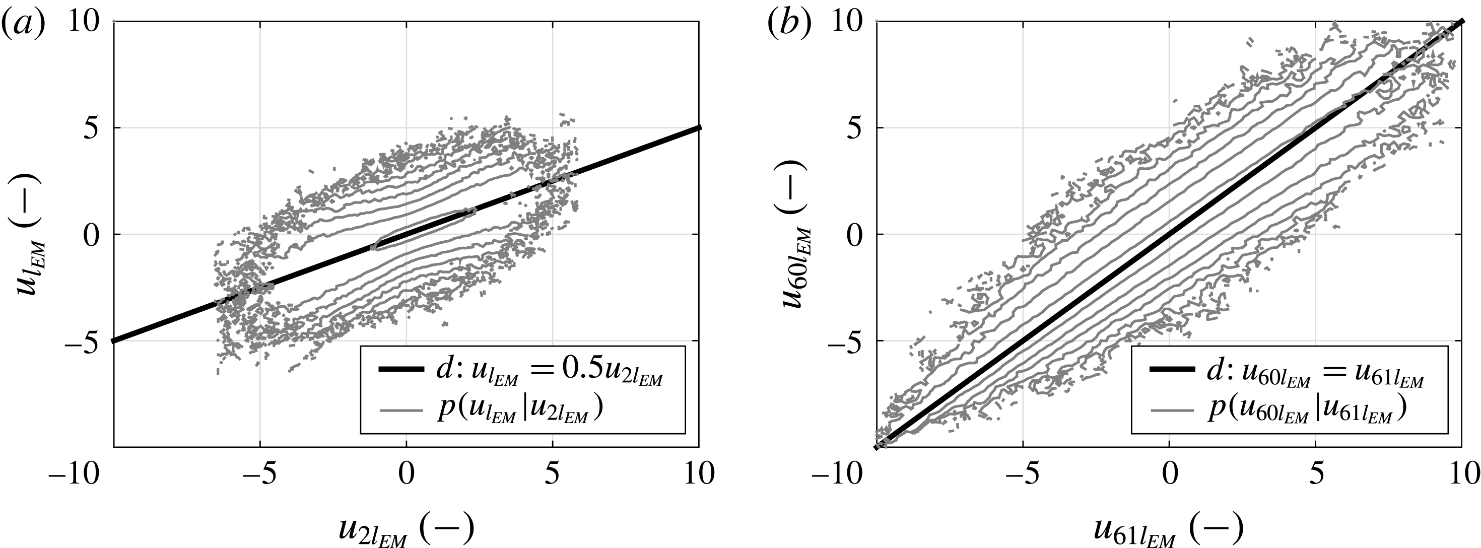
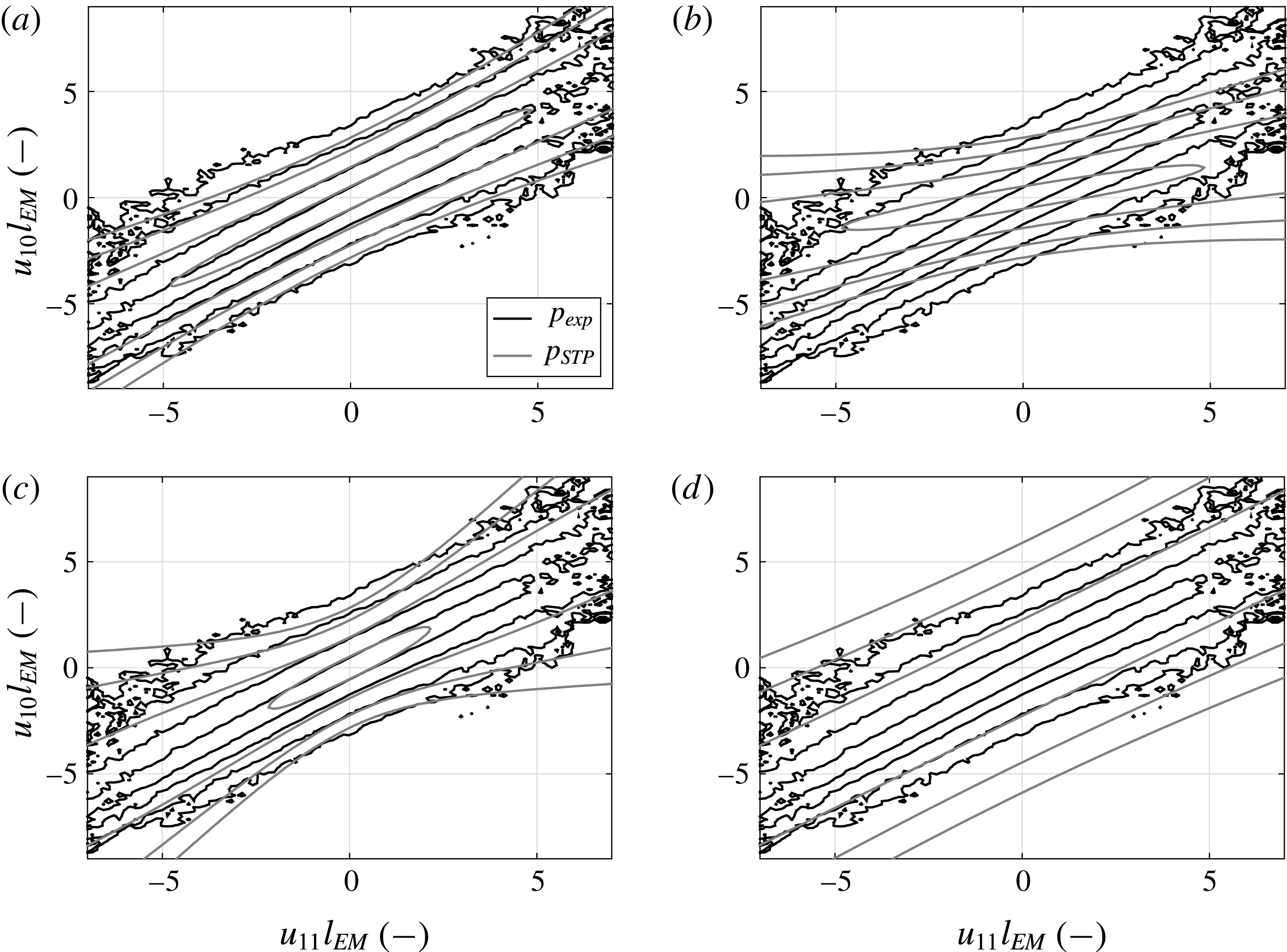
Before we discuss the results in detail, we analyse in figure 9 the topological changes of the conditional PDFs with varying scale, which will serve as a basis for the interpretation of the parameters
 $d_{11}(r),d_{20}(r)$
and
 $d_{22}(r)$
. Figure 9(a) shows an exemplary conditional PDF at a small scale,
 $r=l_{EM}$
. The maximum of the distribution is located at a diagonal of the form
 $d:u_{r}=cu_{r^{\prime }}$
, which is referred to as a distribution diagonal or simply diagonal. Figure 9(a) shows that at scale
 $r=l_{EM}$
, the distribution diagonal is
 $d:u_{l_{EM}}=0.5u_{2l_{EM}}$
. The contour isolines are curved beneath and above this diagonal.
Figure 9(b) shows for the same dataset the conditional PDF at larger scale,
 $r=60l_{EM}$
. (To accentuate the differences between small and large scale,
 $r=60l_{EM}$
is chosen larger than
 $L$
.) The distribution diagonal is now roughly at
 $d:u_{60l_{EM}}=u_{61l_{EM}}$
. The contour isolines are not curved but almost parallel to the diagonal.
These changes in conditional PDF shape can be related to the parameters by considering the short-time propagator (3.17). The leading term for the maximum is given by
 $D^{(1)}$
and
 $d_{11}$
. The smaller the magnitude of
 $d_{11}$
is, the more the diagonal approaches
 $d:u_{r}=u_{r+l_{EM}}$
. The width
 $w$
of the distribution around the diagonal is proportional to the denominator in the exponential term of (3.17),
 $w\propto d_{20}+d_{22}~u_{r+l_{EM}}^{2}$
. Thus, the coefficient
 $d_{22}$
expresses the nonlinearity in the standard deviation and gives rise to the curvature of the contour isolines: the lower
 $d_{22}$
is, the smaller the curvature will be. In terms of unconditional PDF, a large
 $d_{22}$
is equivalent to fat-tailed increment distributions, confirming the previous interpretation that intermittent fluctuations are caused by
 $d_{22}$
. At
 $u_{r+l_{EM}}=0$
, only
 $d_{20}$
characterises the width of the distribution. Further details are discussed in § A.5.
Now, we return to the results for the three parameters
 $d_{11},d_{22}$
and
 $d_{20}$
and their scale dependence. In figure 10, these parameters are shown as a function of the scale
 $r$
and the Taylor–Reynolds number
 $Re_{\unicode[STIX]{x1D706}}$
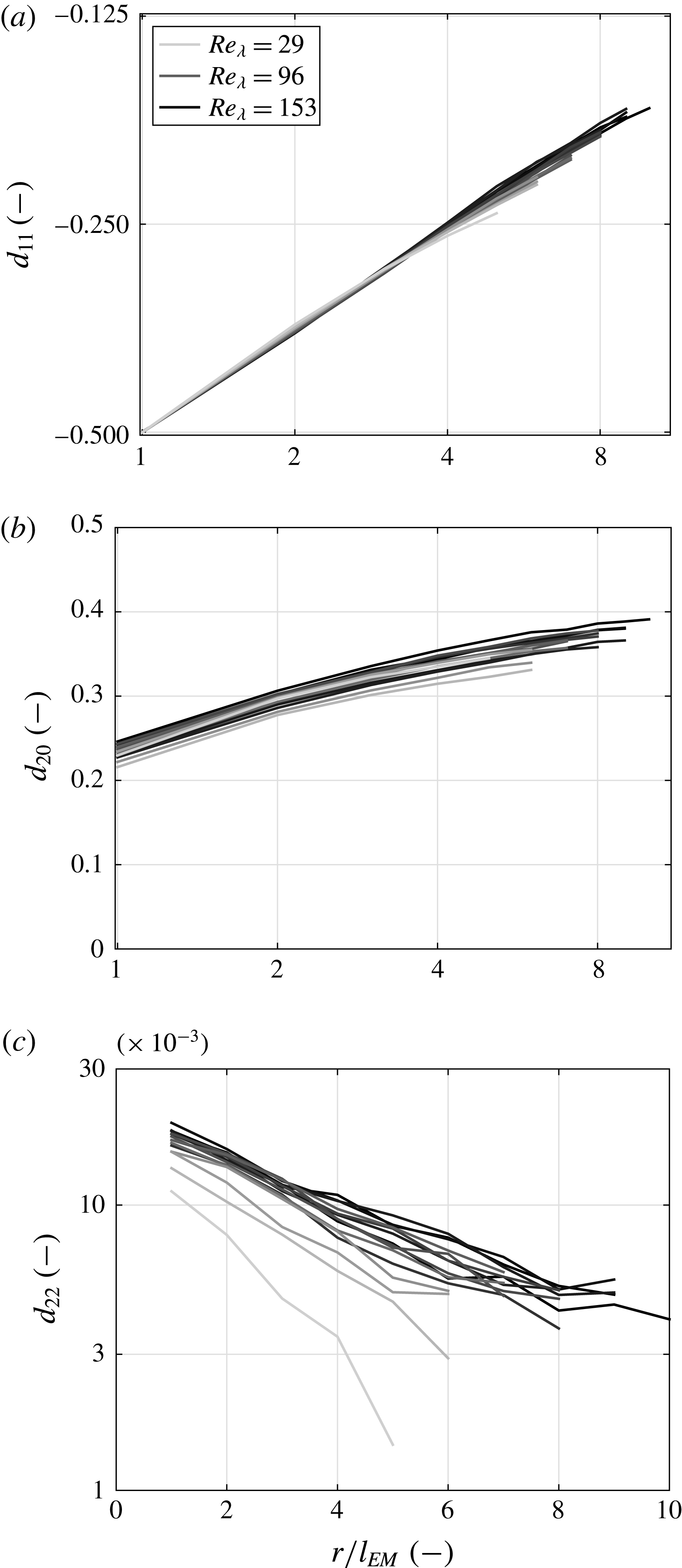
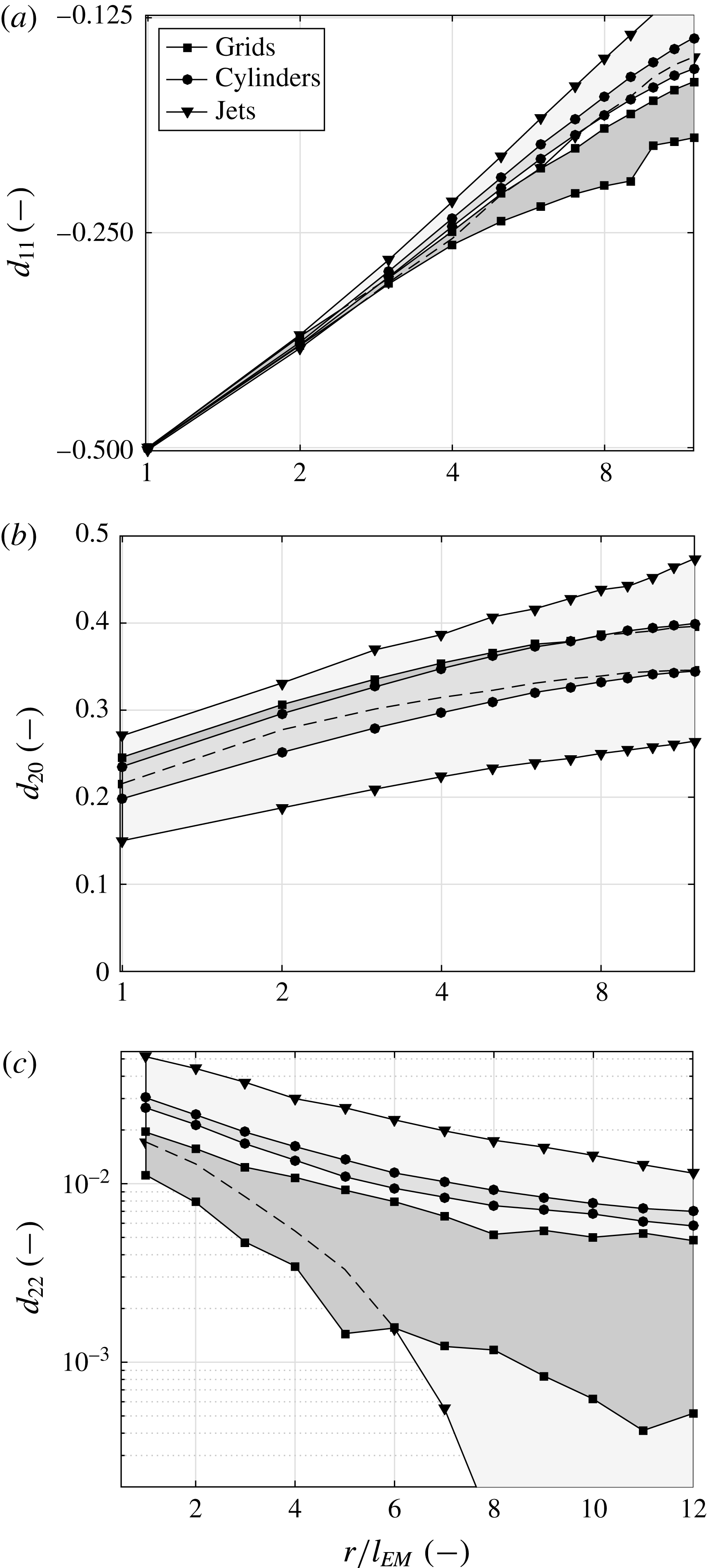
for grid-generated turbulence. Grid data were selected because for these data the smallest scattering was observed. The same presentation of the parameters for cylinder and free-jet flows is shown in § A.6.
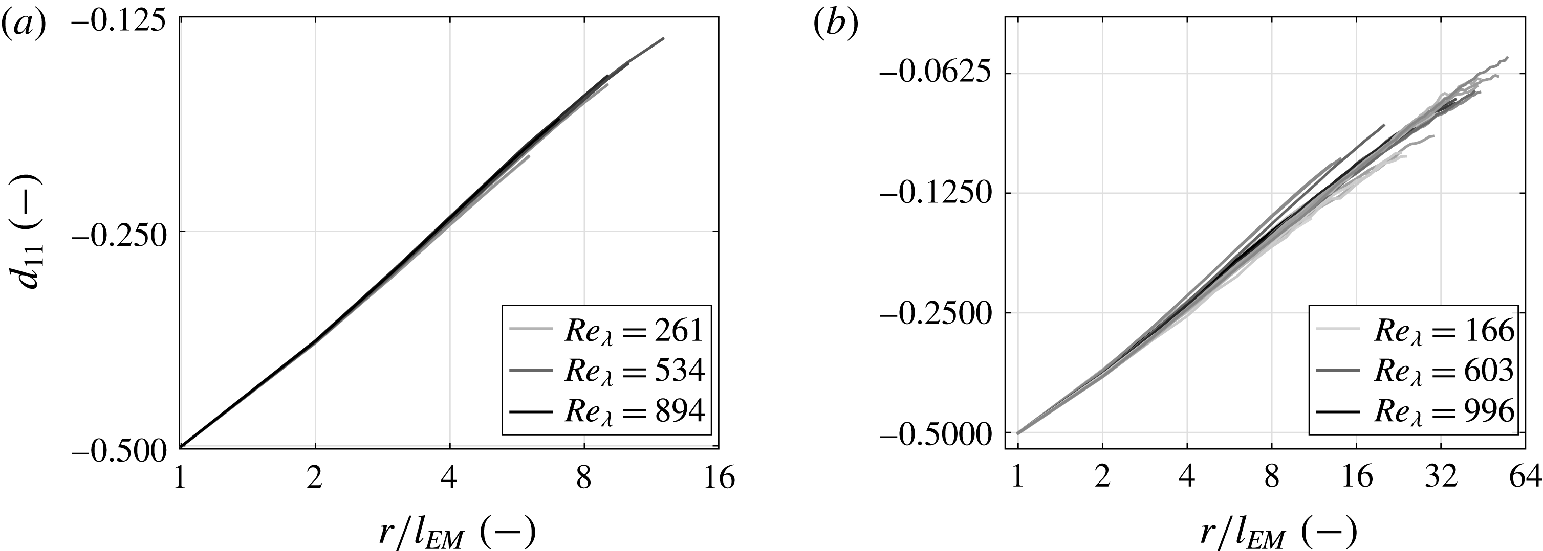
Figure 10(a) shows the convergence of all
 $d_{11}$
to the fixed value
 $d_{11}=-0.5$
at
 $r=l_{EM}$
, which corresponds to a distribution diagonal
 $d:u_{r}=0.5u_{r+l_{EM}}$
, like figure 9(a). Furthermore, all
 $d_{11}$
are approximately linear at small scales in the log–log presentation. Thus,
 $d_{11}$
can be expressed according to
 $$\begin{eqnarray}d_{11}\approx -0.5\left(\frac{r}{l_{EM}}\right)^{-(1/2)}.\end{eqnarray}$$
Equation (4.7) is found to hold universally for all types of flows, as shown in § A.6. The exponent
 $-1/2$
is in accordance with an earlier indication of Renner et al. (Reference Renner, Peinke, Friedrich, Chanal and Chabaud2002b
) for free-jet flows. At larger scales,
 $r\geqslant 4l_{EM}$
, the slope of
 $d_{11}$
decreases slightly and deviations from the power law become visible. The higher
 $Re_{\unicode[STIX]{x1D706}}$
is, the larger the scale where the deviation from the power law sets in is. Thus, (4.7) indicates that the case
 $d:u_{r}=u_{r+l_{EM}}$
is reached only at very large scales and in the limit of very large
 $Re_{\unicode[STIX]{x1D706}}$
.
Parameters of grid-generated turbulence as a function of scale. The greyscale indicates
 $Re_{\unicode[STIX]{x1D706}}$
. (a) Double-logarithmic plot of
 $d_{11}$
. (b) Semi-logarithmic plot of
 $d_{20}$
. (c) Semi-logarithmic plot of
 $d_{22}$
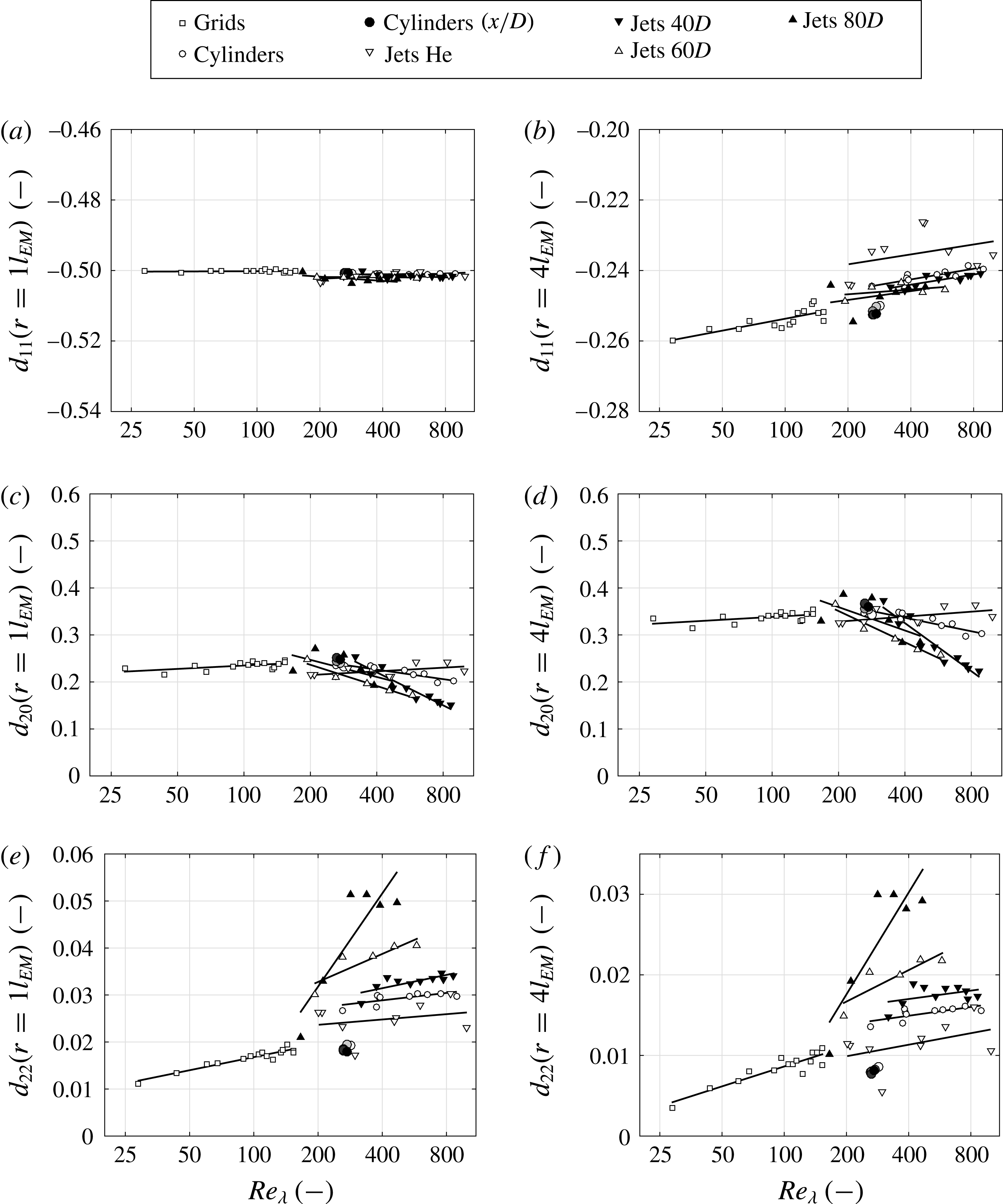
.

Furthermore, the power law with negative exponent (4.7) implies an accelerating decay of turbulent structures along the cascade. From a uniform cascade process, as in the K62 model (3.5), one would expect the power law exponent for
 $d_{11}$
to be
 $-1$
with a prefactor
 ${\approx}-0.36$
, cf. Friedrich & Peinke (Reference Friedrich and Peinke1997a
), Nickelsen (Reference Nickelsen2017). Compared with the K62 process, the smaller exponent
 $-1/2$
found in our analysis together with the prefactor
 $-0.5$
constitutes a decelerated decay of turbulent structures towards smaller scales.
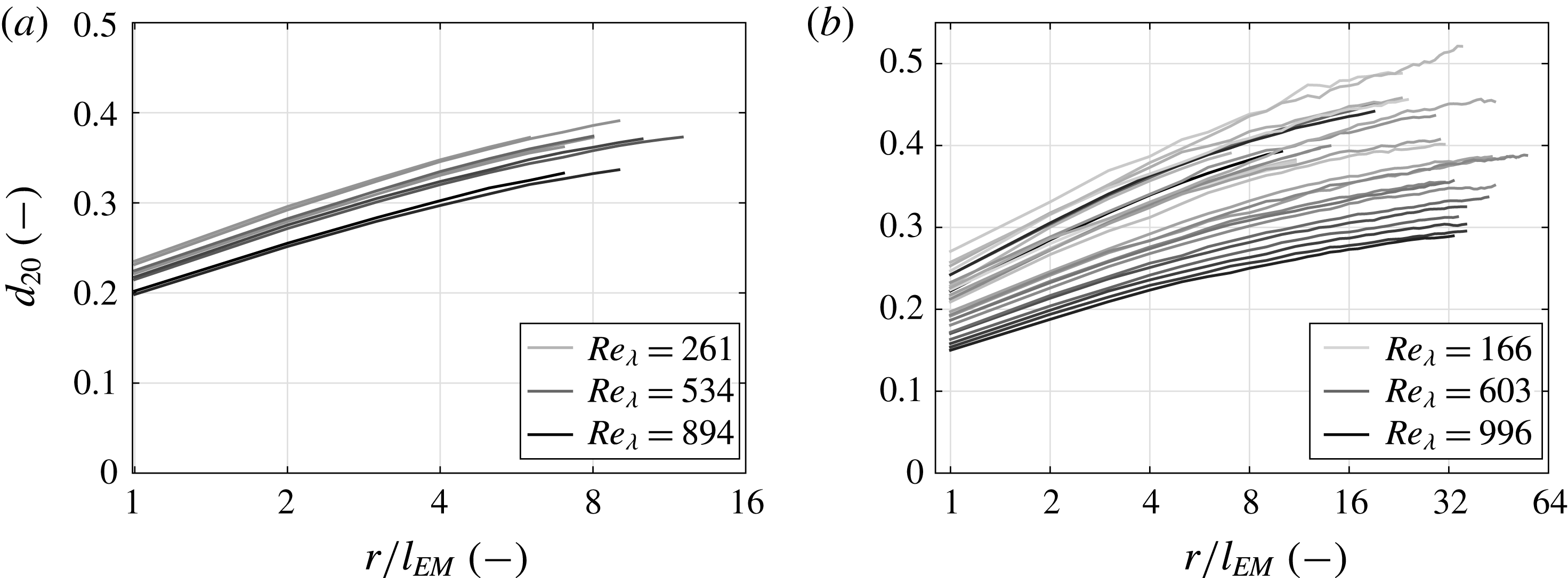
Figure 10(b) presents
 $d_{20}$
in a semi-logarithmic plot. All
 $d_{20}$
show a similar functional form with an increase in scale and a small monotone curvature. The
 $Re_{\unicode[STIX]{x1D706}}$
dependence is rather weak. The functional form can be approximated by
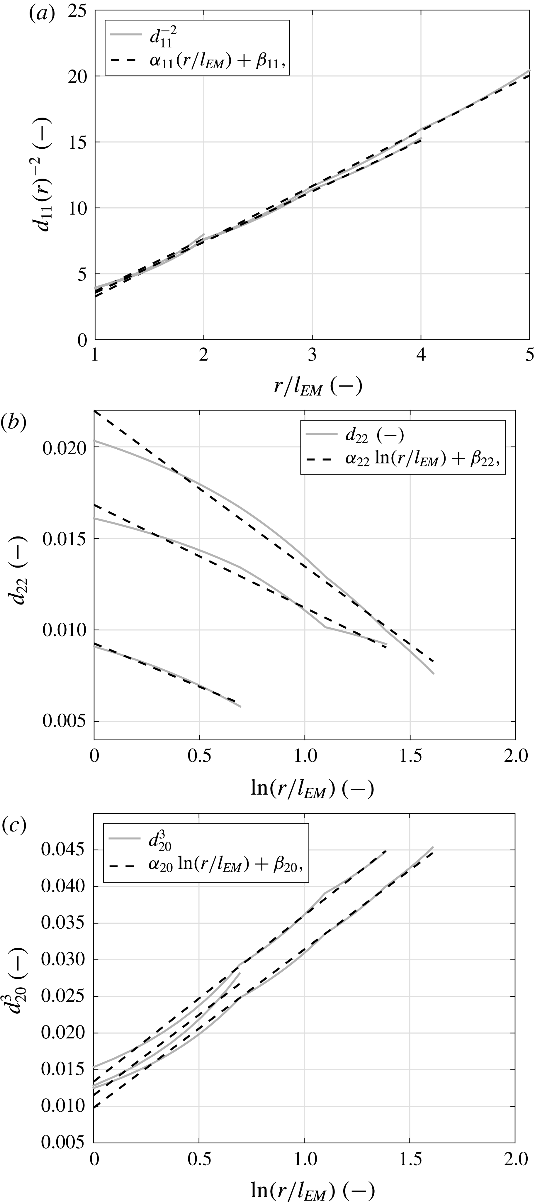
 $$\begin{eqnarray}d_{20}\approx (\unicode[STIX]{x1D6FC}_{20}\ln \left(\frac{r}{l_{EM}}\right)+\unicode[STIX]{x1D6FD}_{20})^{1/3},\end{eqnarray}$$
where
 $\unicode[STIX]{x1D6FC}_{20}$
and
 $\unicode[STIX]{x1D6FD}_{20}$
are fitting parameters, see also § A.4 and figure 16(c). Accordingly, background fluctuations decrease moderately to smaller scales.
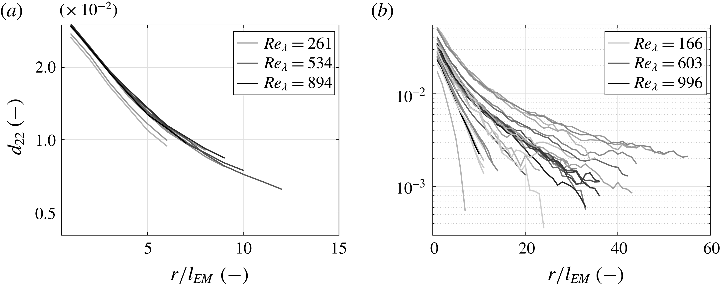
Figure 10(c) presents
 $d_{22}$
in a semi-logarithmic plot. All
 $d_{22}$
decrease strongly with increasing scale, with a slower decrease for increasing
 $Re_{\unicode[STIX]{x1D706}}$
. This functional behaviour can be approximated by
 $$\begin{eqnarray}d_{22}\approx \unicode[STIX]{x1D6FC}_{22}\ln \left(\frac{r}{l_{EM}}\right)+\unicode[STIX]{x1D6FD}_{22},\end{eqnarray}$$
where
 $\unicode[STIX]{x1D6FC}_{22}$
and
 $\unicode[STIX]{x1D6FD}_{22}$
are fitting parameters, see also § A.4 and figure 16(b). In contrast to
 $d_{20}$
,
 $d_{22}$
increases strongly to smaller scales. Since
 $d_{22}$
is the magnitude of the
 $u^{2}$
term in
 $D^{(2)}$
, intermittent features also increase towards smaller scales, establishing the link to small-scale intermittency.
The above parametrisation also allows a qualitative discussion of the infinite-Reynolds-number limit. From figures 10, 12 and 19–21, it can be concluded that
 $d_{11}$
and
 $d_{20}$
appear to be rather independent of
 $Re_{\unicode[STIX]{x1D706}}$
. For
 $d_{11}$
, this independence is apparent; for
 $d_{20}$
, one may also see a decreasing tendency with
 $Re_{\unicode[STIX]{x1D706}}$
, which was also found in Renner et al. (Reference Renner, Peinke and Friedrich2002
a
). In contrast,
 $d_{22}$
clearly increases with
 $Re_{\unicode[STIX]{x1D706}}$
, confirming that small-scale intermittency intensifies with
 $Re_{\unicode[STIX]{x1D706}}$
. A direct quantitative analysis in terms of the intermittency factor
 $\unicode[STIX]{x1D707}$
is questionable due to non-scaling behaviour (Renner et al.
Reference Renner, Peinke and Friedrich2002
a
, figure 4b), but qualitatively it follows from (3.11) that
 $\unicode[STIX]{x1D707}(r)=18d_{22}(r)$
, neglecting
 $d_{20}$
and taking
 $d_{11}$
and
 $d_{22}$
as the K62 contribution. The resulting local intermittency factor,
 $\unicode[STIX]{x1D707}(r)$
, indeed increases with
 $Re_{\unicode[STIX]{x1D706}}$
from
 $\unicode[STIX]{x1D707}=0.2$
to
 $\unicode[STIX]{x1D707}=0.4$
at
 $r=l_{EM}$
, and from
 $\unicode[STIX]{x1D707}=0.1$
to
 $\unicode[STIX]{x1D707}=0.3$
at
 $r=3l_{EM}$
, in qualitative agreement with the universal value of
 $\unicode[STIX]{x1D707}\approx 0.26$
.
We continue with an analysis regarding the universality of the functional forms of
 $d_{11}$
,
 $d_{20}$
and
 $d_{22}$
. Figure 11 shows the three parameters for all datasets in logarithmic plots. The parameters are sorted into three groups which reflect the different turbulent flow types. All parameters that belong to grid flows, cylinder flows or free-jet flows are covered by a surface with different greyscale and are enclosed by different symbols. Dashed lines indicate where edges are overlaid. In addition, figure 12 shows the parameters as a function of the Taylor–Reynolds number at the fixed scales
 $r=l_{EM}$
and
 $r=4l_{EM}$
.
The parameters
 $d_{11}$
,
 $d_{20}$
and
 $d_{22}$
as a function of scale. Surfaces indicate areas where the parameters of specific turbulent flow are located. (a) Double-logarithmic plot of
 $d_{11}$
. (b) Semi-logarithmic plot of
 $d_{20}$
. (c) Semi-logarithmic plot of
 $d_{22}$
.

At small scales, all
 $d_{11}$
converge to an approximate power law with the exponent
 $-0.5$
at
 $r\gtrsim l_{EM}$
, as shown in figure 11(a). Therefore, universal scaling features of
 $d_{11}$
are found for our datasets at small scales, which is confirmed by plotting the
 $Re_{\unicode[STIX]{x1D706}}$
dependence of
 $d_{11}(r=l_{EM})$
, see figure 12(a). At larger scales, the three groups broaden differently and start to deviate from the power law behaviour. Figure 12(b) indicates that the different behaviour in
 $d_{11}$
is mainly an
 $Re_{\unicode[STIX]{x1D706}}$
effect and does not show significant differences for the different flows. More specifically, at small scales,
 $d_{11}$
acquires a universal form, which shows a dependence on neither the kind of turbulent flow nor
 $Re_{\unicode[STIX]{x1D706}}$
, and at larger scales,
 $Re_{\unicode[STIX]{x1D706}}$
becomes important, but the kind of flow does not have a strong effect on
 $d_{11}$
features.
Parameters as a function of
 $Re_{\unicode[STIX]{x1D706}}$
at two fixed scales (
 $r=l_{EM}$
and
 $4l_{EM}$
). Additionally, linear fit functions indicate trends. All plots are semi-logarithmically plotted.

Figure 11(b) shows
 $d_{20}$
. The three groups of flows increase with scale in a similar manner to that for
 $d_{11}$
. As a further characterisation, we show the
 $Re_{\unicode[STIX]{x1D706}}$
dependence of
 $d_{20}$
again for the same two scales in figure 12(c,d). The overall trend of the entire collection of datasets is rather constant and subgroups overlap. Thus, a quite uniform band of data is found. It should be noted that
 $d_{20}$
is sensitive to the normalisation of the velocity increment series (3.7). On the one hand, a more sophisticated norm based on
 $d_{20}$
might result in a perfect collapse of the
 $d_{20}(r)$
, at least at one scale. On the other hand, a norm
 $\unicode[STIX]{x1D70E}_{\infty }=\sqrt{2}\unicode[STIX]{x1D70E}(v)$
would lead to a distinct dependence of
 $d_{20}$
on
 $Re_{\unicode[STIX]{x1D706}}$
. We hence stick to the normalisation using
 $\unicode[STIX]{x1D6E9}$
and
 $\unicode[STIX]{x1D70E}_{\unicode[STIX]{x1D6E9}}$
to deliver a uniform picture in the two-point and multipoint analysis, which entails the displayed weak dependence of
 $d_{20}$
on
 $Re_{\unicode[STIX]{x1D706}}$
, and which therefore supports our choice to use the new quantities
 $\unicode[STIX]{x1D6E9}$
and
 $\unicode[STIX]{x1D70E}_{\unicode[STIX]{x1D6E9}}$
for normalisation.
Regarding
 $d_{22}$
, the turbulent flows divide into distinct groups, as shown in figure 11(c). These groups are different in shape and broadness, where, from bottom to top, the functional form of the group borders changes in a quite systematic way. To investigate whether this behaviour can be explained by a
 $Re_{\unicode[STIX]{x1D706}}$
dependence or not, we proceed as above by plotting
 $d_{22}(r=l_{EM})$
and
 $d_{22}(r=4l_{EM})$
as a function of
 $Re_{\unicode[STIX]{x1D706}}$
, see figure 12(e,f). In contrast to the findings for
 $d_{11}$
and
 $d_{20}$
, the data do not collapse on a uniform
 $Re_{\unicode[STIX]{x1D706}}$
behaviour, but clearly distinct dependences can be seen. Each dataset seems to follow a different evolution with
 $Re_{\unicode[STIX]{x1D706}}$
. Most interestingly, this also holds for the case of small scales
 $r=l_{EM}$
, for which a convergence to a flow-type independent behaviour should be expected in the common understanding of universal turbulence.
We further extend our research and try to combine the various subgroups of
 $d_{22}$
. If we plot the parameter
 $d_{22}$
as a function of the dimensionless length
 $L/\unicode[STIX]{x1D706}$
instead of
 $Re_{\unicode[STIX]{x1D706}}$
, it may allow us to combine the subgroups within the flow types, i.e. free-jet data become more aligned, see figure 22 in § A.7. However, the different flow types themselves cannot be combined into one universal functional form.
5 Conclusion
In the common understanding of turbulence, large-scale structures, where energy is fed into a cascade process, are known to be dependent on the generating process. For small structures, it is commonly believed that they have flow-independent features. This assumption of universal small-scale structures is utilised in turbulence modelling. It is the objective of this paper to discuss to what degree such a universal behaviour is present. Therefore, we performed a comprehensive investigation based on two-point statistics (i.e. structure functions), multiscale statistics (i.e. Markov analysis) and the analogue thermodynamic process (i.e. IFT), as well as 61 different turbulent flows with various kinds of turbulence generation.
Our first analysis step of the extensive dataset confirms the common 2-point statistics’ scaling picture of homogeneous isotropic turbulence, cf. Kolmogorov (Reference Kolmogorov1962), figure 1. Furthermore, a closer investigation of local scaling exponents of structure functions and its features is also set in a universal dependence on
 $Re_{\unicode[STIX]{x1D706}}$
, which is supported by results of Mydlarski & Warhaft (Reference Mydlarski and Warhaft1996), figure 2. The shown results do not allow a distinction between the different turbulent flows and no significant clustering with regard to the generation of turbulence could be detected. These results and their scattering are in agreement with other studies, e.g. Gylfason & Warhaft (Reference Gylfason and Warhaft2004), and confirm the common picture of universal small-scale turbulence.
For this traditional scaling analysis of structure functions, we introduced two new quantities,
 $\unicode[STIX]{x1D6E9}$
and
 $\unicode[STIX]{x1D70E}_{\unicode[STIX]{x1D6E9}}$
, for the purpose of normalisation of scale and magnitudes of structure functions as in (3.7). As these quantities are dimensional and contain information on large-scale structures, we achieved a comparable basis and a collapse of the data for all considered turbulent flows.
After we had put our results in the context of the common understanding of turbulence, we continued with an advanced study which included joint multiscale statistics and the utilisation of the IFT as a consequence of the interpretation of the turbulent cascade as a non-equilibrium thermodynamic process.
As a first main result, we were able to show the validity of the IFT for all datasets, equation (3.23) and figure 7. The high quality of the validity of the IFT led us to propose that the IFT can be taken as a new general law for the turbulent cascade. Furthermore, utilising the IFT in combination with a self-consistent optimisation procedure, we were able to work out the significant functional contributions to the stochastic cascade process, see (3.15), (3.16) and figure 10. For all data, we see that these contributions are given by three aspects and parameters.
A deterministic part, expressed by
 $d_{11}(r)$
in (4.7), corresponds to a returning force which pulls increments to the equilibrium state
 $u=0$
while the cascade proceeds towards smaller scales. Thus, the deterministic part describes the reduction of the magnitude of the increments
 $u_{r}$
with decreasing scales and fixes the average tendency of the cascade. The functional form of
 $d_{11}$
in scale follows a power law, where the scaling exponent indicates, compared with the K62 model (3.5), a decelerated decay of turbulent structures towards smaller scales.
Stochastic forces are represented by an additive and a multiplicative noise term, given by
 $d_{20}(r)$
and
 $d_{22}(r)$
in (4.8) and (4.9) respectively. Both stochastic forces add fluctuations to the deterministic evolution of increments and counteract the equilibrium tendency of the deterministic part. However, both are quite different in their significance and nature. The additive noise term
 $d_{20}$
adds background fluctuations independent of
 $u_{r}$
, with a noticeable decrease with decreasing scale. In contrast, the multiplicative noise term
 $d_{22}$
incorporates the energetic term
 $u^{2}$
as a source of fluctuations, just as the thermal energy of a reservoir is a source of fluctuations in a thermodynamic process. As
 $d_{22}$
increases with decreasing scale, heavy tails of PDFs grow and extreme events become more likely towards smaller scales. This result is in agreement with the evolution of the energy transfer rate along the cascade, which starts off with a non-fluctuating average large value and becomes more and more fluctuating towards smaller scales. The increasing occurrence of extreme events is responsible for the phenomenon of small-scale intermittency, and it is important to note that these fluctuations do not occur haphazardly but are well balanced with average realisations of the cascade process as checked by the IFT.
Our analysis demonstrated in particular that these three contributions are sufficient to also reproduce the measured evolution of skewness along the cascade in compliance with the four-fifths law, cf. figure 6. In other words, due to the absence of a term
 $d_{21}$
, the two stochastic forces do not need to be correlated for the correct inclusion of skewness, contrary to many other stochastic models. Instead, with the additive noise acting predominantly on large scales and the multiplicative noise on small scales, an intuitive fluid dynamic picture of the turbulent cascade is conveyed: the additive noise injects energy on large scales, the linear drift is responsible for the transfer down the cascade and the multiplicative noise effectively damps the fluctuations (weak noise for small
 $u$
), superimposed by intermittent outbursts (strong noise for large
 $u$
). In this picture, it is the linear drift term
 $d_{11}$
that is responsible for the correct evolution of initial large-scale skewness along the cascade.
The second main result is the reduction of the stochastic model to these three influences and their interpretation. Adding to that, the derived stochastic cascade model (based on the three parameters) leads to a closed set of differential equations for structure functions, (4.6), which allows a decent reproduction of structure functions and includes correct deviations from usual scaling behaviour, e.g. (Kolmogorov Reference Kolmogorov1962).
Owing to our finding that the stochastic cascade process of turbulence can be represented by scale-dependent parameters
 $d_{ij}$
, we were able to investigate the aspects of universality in detail, figures 11 and 12. We found that the evolutions in scale of
 $d_{11}$
and
 $d_{20}$
are universal in the sense that they are flow-independent. Thus, their functional forms can be expressed by scale and/or
 $Re_{\unicode[STIX]{x1D706}}$
dependences.
Our third main result is that in strong contrast to the findings for the structure functions and the parameters
 $d_{11}$
and
 $d_{20}$
, the parameter
 $d_{22}$
as a function of
 $Re_{\unicode[STIX]{x1D706}}$
splits up into distinct clusters for every considered dataset subgroup, which are characterised by specific large-scale flow structures and the turbulence generation mechanism. Thus, we conclude that specific turbulent flows have their own particular multiscale cascades, in other words, their own stochastic fingerprints.
Acknowledgements
We would like to acknowledge the funding from DFG and the cooperation as well as discussions with D. Bastine, A. Engel, A. Hadjihosseini, P. Lind, P. Milan, R. Stresing, M. R. R. Tabar and M. Wächter as well as the experimental datasets provided by O. Chanal, St. Lück and Ch. Renner. J.P. acknowledges support from the Laboratoire d’excellence LANEF in Grenoble (ANR-10-LABX-51-01)
Appendix A
A.1 Determination of integral length
The determination of the integral length is based on the definition in Batchelor (Reference Batchelor1953, p. 47), where the autocorrelation
 $R(r)$
is integrated from zero to infinity. From a particle point of view, the integration is stopped before infinity; thus, an upper limit
 $r_{up}$
is needed. For our data, we investigate, going from zero to larger scales, whether the autocorrelation decreases monotonically with
 $\unicode[STIX]{x2202}_{r}R(r)\leqslant 0$
and
 $\unicode[STIX]{x2202}_{rr}R(r)\geqslant 0$
. For this case, the integration is performed up to
 $R(r)\leqslant 0.01$
. If this is not the case, an
 $r_{up}$
is defined at the location where the monotonic decrease is violated. After
 $r=r_{up}$
, the autocorrelation function becomes extrapolated, as inspired by Batchelor (Reference Batchelor1953, pp. 92–96, figure 5.2),
 $$\begin{eqnarray}L=\displaystyle \int _{0}^{r_{up}}R(r)\,\text{d}r+\frac{\text{e}^{a\cdot r_{up}+b}}{a}.\end{eqnarray}$$
The parameters
 $a$
and
 $b$
are obtained by a fitting routine. The fitting range is between
 $r_{low}$
and
 $r_{up}$
. The low border
 $r_{low}$
is chosen as the larger value of
 $R(r_{low})=2/e$
or
 $3R(r_{up})$
. Figure 13(a) exemplarily illustrates this procedure. Figure 13(b) shows the integral length
 $L$
in units of the Taylor microscale
 $\unicode[STIX]{x1D706}$
versus the Taylor based Reynolds number. For all subgroups of datasets, the ratio
 $L/\unicode[STIX]{x1D706}$
increases with
 $Re_{\unicode[STIX]{x1D706}}$
, as highlighted by linear fits. The relation
 $L/\unicode[STIX]{x1D706}\propto Re_{\unicode[STIX]{x1D706}}$
can be derived from
 $L\approx$
constant,
 $\unicode[STIX]{x1D706}\propto R\text{e}^{-(1/2)}$
and
 $Re_{\unicode[STIX]{x1D706}}\propto Re^{1/2}$
, cf. Lück et al. (Reference Lück, Renner, Peinke and Friedrich2006). It should be noted that, in figure 13(b), a double-logarithmic presentation is used for reasons of clarity.
(a) Illustration of the procedure for determining the integral length. The autocorrelation function, the considered part (solid black line) and the neglected part (dashed black line), the range of fit(open circles) and the extrapolation of
 $R(r)$
(grey solid line) are shown. (b) The length of the inertial range
 $L/\unicode[STIX]{x1D706}$
as a function of
 $Re_{\unicode[STIX]{x1D706}}$
for all datasets.

A.2 Einstein–Markov coherence length
The Einstein–Markov coherence length
 $l_{EM}$
is a length at which
 $$\begin{eqnarray}\displaystyle & \displaystyle p(u_{r}|u_{r+l_{\unicode[STIX]{x1D6E5}}})=p(u_{r}|u_{r+l_{\unicode[STIX]{x1D6E5}}},u_{r+2l_{\unicode[STIX]{x1D6E5}}}=0\pm \unicode[STIX]{x1D712}), & \displaystyle\end{eqnarray}$$
 $$\begin{eqnarray}\displaystyle & \displaystyle \unicode[STIX]{x1D712}=0.1\unicode[STIX]{x1D70E}_{v} & \displaystyle\end{eqnarray}$$
is fulfilled. Lück et al. (Reference Lück, Renner, Peinke and Friedrich2006) used the Wilcoxon test to verify this length, which can be considered as a linear measure. Here, a test is used that is based on (3.18). Since (3.18) is a logarithmic measure, rare events are more strongly weighted. Figure 14 shows an exemplary examination of (A 2) under variation of
 $\unicode[STIX]{x1D6E5}$
, which is given in units of
 $\unicode[STIX]{x1D706}$
. The first steep part of
 $\unicode[STIX]{x1D716}$
is extrapolated to estimate
 $l_{EM}$
. A first-order polynomial (
 $O=1$
) leads to a similar result to that published by Lück et al. (Reference Lück, Renner, Peinke and Friedrich2006) and a second-order polynomial (
 $O=2$
) leads to a higher estimation of
 $l_{EM}\approx 2\unicode[STIX]{x1D706}$
. For both estimations (
 $O=1$
and
 $O=2$
) of
 $l_{EM}$
, a non-Markovian share remains. It should be noted that the relation between
 $l_{EM}$
and
 $\unicode[STIX]{x1D706}$
slightly changes the IFT convergence,
 $l_{EM}=\unicode[STIX]{x1D706}\rightarrow \langle I_{max}\rangle \approx 1.02$
and
 $l_{EM}=2\unicode[STIX]{x1D706}~\rightarrow \langle I_{max}\rangle \approx 1.01$
.


(a) The norm
 $\unicode[STIX]{x1D6E9}$
versus
 $Re_{\unicode[STIX]{x1D706}}$
in a double-logarithmic plot. (b) The norm
 $\unicode[STIX]{x1D70E}_{\unicode[STIX]{x1D6E9}}$
versus
 $Re_{\unicode[STIX]{x1D706}}$
. Both norms are shown for all datasets. Trends are highlighted by linear fitting functions.

Plot of
 $d_{ij}$
in a linearised form as well as fitting functions. The length of
 $d_{ij}$
corresponds to
 $Re_{\unicode[STIX]{x1D706}}$
, see table 3.

A.3 Characterisation of norms
Figure 15 shows the dimensional norms
 $\unicode[STIX]{x1D6E9}$
and
 $\unicode[STIX]{x1D70E}_{\unicode[STIX]{x1D6E9}}$
as a function of
 $Re_{\unicode[STIX]{x1D706}}$
. Here,
 $\unicode[STIX]{x1D6E9}$
is plotted in a double-logarithmic fashion; thereby, a power law dependence on
 $Re_{\unicode[STIX]{x1D706}}$
becomes evident. The term
 $\unicode[STIX]{x1D70E}_{\unicode[STIX]{x1D6E9}}$
depends linearly on
 $Re_{\unicode[STIX]{x1D706}}$
, figure 15(b). For both quantities, the different generated flows show up in individual clusters, which are, interestingly, arranged in different ways. Although
 $\unicode[STIX]{x1D6E9}$
and
 $\unicode[STIX]{x1D70E}_{\unicode[STIX]{x1D6E9}}$
are connected by their definitions, the different arrangements and the different functional dependences on
 $Re_{\unicode[STIX]{x1D706}}$
show that they are not trivially linked to one another. The ratio
 $\unicode[STIX]{x1D6E9}/\unicode[STIX]{x1D706}$
(e.g. as function of
 $Re_{\unicode[STIX]{x1D706}}$
) shows a rather scattered distribution: values are between
 $2$
and
 ${\sim}4$
; however, some ratios go up to
 ${\sim}7$
.
A.4 Structure functions deduced by
$D^{(1,2)}$

Equation (4.6) allows us to calculate the structure functions and
 $\unicode[STIX]{x1D709}_{\unicode[STIX]{x1D705}}(r)$
from the parameters
 $d_{ij}$
. Figure 16 shows our approaches to proper parametrisations according to
 $d_{11}=(\unicode[STIX]{x1D6FC}_{11}r/l_{EM}+\unicode[STIX]{x1D6FD}_{11})^{-1/2}$
,
 $d_{22}=\unicode[STIX]{x1D6FC}_{22}\ln (r/l_{EM})+\unicode[STIX]{x1D6FD}_{22}$
and
 $d_{20}=(\unicode[STIX]{x1D6FC}_{20}\ln (r/l_{EM})+\unicode[STIX]{x1D6FD}_{20})^{1/3}$
. For this illustration, three different datasets are used. The
 $Re_{\unicode[STIX]{x1D706}}$
values and the corresponding fit parameters
 $\unicode[STIX]{x1D6FC}_{ij}$
and
 $\unicode[STIX]{x1D6FD}_{ij}$
as well as the flow types are summarised in table 3.
The
 $d_{ij}$
parametrisation in terms of
 $\unicode[STIX]{x1D6FC}_{ij}$
and
 $\unicode[STIX]{x1D6FD}_{ij}$
; see also table 1.

The local scaling exponents are shown in figure 17, and are deduced directly from the velocity increments and the parameters using (4.6). The values of the optimised
 $D^{(1,2)}$
as well as the mentioned fit functions of the parameters
 $d_{ij}$
are used. Here, as an exception, we use
 $l_{EM}=\unicode[STIX]{x1D706}$
to highlight the crossing of K62. It should be noted that the jumpy development of
 $\unicode[STIX]{x1D709}_{\unicode[STIX]{x1D705}}$
is caused by a linear interpolation of
 $D^{(1,2)}$
. An error margin
 $\unicode[STIX]{x0394}\unicode[STIX]{x1D709}_{\unicode[STIX]{x1D705}}(r)$
of
 $\unicode[STIX]{x1D709}_{\unicode[STIX]{x1D705}}(r)$
is derived from the experimental data. This is done by splitting the measured data into
 $n$
groups and determining
 $n$
times
 $\unicode[STIX]{x1D709}_{\unicode[STIX]{x1D705}}(r)$
, from which the standard deviation
 $\unicode[STIX]{x1D70E}(\unicode[STIX]{x1D709}_{\unicode[STIX]{x1D705}}^{n}(r))$
is calculated. In this way (
 $n=50$
),
 $$\begin{eqnarray}\displaystyle \unicode[STIX]{x0394}\unicode[STIX]{x1D709}_{\unicode[STIX]{x1D705}}(r)=\frac{\unicode[STIX]{x1D70E}(\unicode[STIX]{x1D709}_{\unicode[STIX]{x1D705}}^{n}(r))}{\sqrt{n}} & & \displaystyle\end{eqnarray}$$
is determined. As an orientation, also Kolmogorov’s prediction according to (3.5) is shown, labelled K62, similarly to figure 2(a).
The local scaling exponent
 $\unicode[STIX]{x1D709}_{\unicode[STIX]{x1D705}}(r)$
deduced from experimental data, reconstructed by
 $D^{(1,2)}$
as well as their fits. Kolmogorov’s prediction is also shown (K62) and an error margin of the experimental data. Grid (i) is used as an exemplary dataset, characterised in tables 1 and 3.

A.5 Interpretation of
$D^{(1)}$
and
$D^{(2)}$
with the short-time propagator


The interpretation of
 $D^{(1,2)}$
and
 $d_{11}$
,
 $d_{22}$
,
 $d_{20}$
is made by modifying the optimised
 $D^{(1,2)}$
and presenting the corresponding short-time propagator. The short-time propagator deduced by unmodified
 $d_{11}$
,
 $d_{22}$
and
 $d_{20}$
(regular optimised) is shown in figure 18(a). The agreement is good between the short-time propagator and the experimental reference data. In figure 18(b),
 $d_{11}$
is multiplied by 5, whereas
 $d_{22}$
and
 $d_{20}$
are unmodified. This multiplication twists the diagonal of the short-time propagator in comparison to the experimental reference data. Thus, we see that the magnitude of
 $d_{11}$
controls the diagonal. In figure 18(c),
 $d_{22}$
is multiplied by 5, whereas
 $d_{11}$
and
 $d_{20}$
are unmodified. An enlarged
 $d_{22}$
increases the curvature of the isolines in the contour plot. Therefore, the probability for extreme events increases, which is equivalent to an increased intermittency and to more fat-tailed unconditional PDFs. In figure 18(d),
 $d_{20}$
is multiplied by 5, whereas
 $d_{11}$
and
 $d_{22}$
are unmodified. Here, the reconstructed distribution becomes broader around the distribution diagonal.
One exemplary experimentally found conditional PDF,
 $p_{exp}$
(black) (subgroup (v),
 $Re_{\unicode[STIX]{x1D706}}=475$
), and four different results of the short-time propagator
 $p_{STP}$
(grey). (a) The short-time propagator regarding the optimised
 $D^{(1,2)}$
. (b) The same as in (a) except that
 $d_{11}$
is multiplied by 5. (c) Only
 $d_{22}$
is multiplied by 5. (d) Only
 $d_{20}$
is multiplied by 5.

A.6 Single developments of
$d_{11}$
,
$d_{22}$
and
$d_{20}$
in scale


For the sake of completeness, the coefficients
 $d_{11}$
,
 $d_{22}$
and
 $d_{20}$
are shown for cylinder and free-jet flows as a function of scale in figures 19–21. These figures are just the same as figure 10.
Plot of
 $d_{11}$
as a function of scale, for cylinder flows (a) and free-jet flows (b). The greyscale of the lines indicates
 $Re_{\unicode[STIX]{x1D706}}$
.

Plot of
 $d_{20}$
as a function of scale, for cylinder flows (a) and free-jet flows (b). The greyscale of the lines indicates
 $Re_{\unicode[STIX]{x1D706}}$
.

Plot of
 $d_{22}$
as a function of scale, for cylinder flows (a) and free-jet flows (b). The greyscale of the lines indicates
 $Re_{\unicode[STIX]{x1D706}}$
.

A.7 The parameter
$d_{22}$
as a function of
$L/\unicode[STIX]{x1D706}$


The findings of figure 12(e,f) can be further investigated in terms of universality by interpreting
 $d_{22}$
as a function of a different quantity, for instance by plotting
 $d_{22}$
as a function of the dimensionless length
 $L/\unicode[STIX]{x1D706}$
, which is the relative length of the inertial range. The results become newly sorted and give a much more uniform picture, see figure 22(a,b). Although single free-jet subgroups might be systematically distinguished in terms of the relative distance to the nozzle, the entire free-jet datasets show a rather uniform group, in contrast to figure 12(e,f). The relative location of the cylinder subgroup differs clearly from the other data in this presentation. Although
 $d_{22}$
is more sorted, we come to the same conclusion as above: intermittency features in terms of
 $d_{22}$
are non-universal, and single flow types become apparent.
The parameter
 $d_{22}$
as a function of
 $L/\unicode[STIX]{x1D706}$
at two fixed scales (
 $r=l_{EM}$
and
 $4l_{EM}$
). Additionally, linear fitting functions indicate trends. The plots are semi-logarithmically plotted.