















1. Introduction
Wind-fed accretion onto magnetised neutron stars (NSs) is common in high-mass X-ray binaries (HMXBs), where compact objects capture material from the fast, radiatively driven winds of OB donors. Symbiotic X-ray binaries (SyXBs), which host evolved cool giants or supergiants with slow, dense winds, are much rarer but provide an important regime for studying angular-momentum transfer and torque noise in structured, low-velocity outflows (e.g. Masetti et al. Reference Masetti2007; Lü et al. Reference Lü2012; Hinkle et al. Reference Hinkle2020; Yungelson et al. Reference Yungelson, Kuranov and Postnov2019). Among wind-accreting NS systems, 4U 1954+319 is notable in that it hosts the slowest known accretion-powered pulsar (
 $P_\mathrm{s}\sim5.4$
h) and an M-type supergiant donor (Masetti et al. Reference Masetti, Orlandini, Palazzi, Amati and Frontera2006, Reference Masetti2007; Mattana et al. Reference Mattana2006; Hinkle et al. Reference Hinkle2020).
At the low and intermediate X-ray luminosities usually associated with 4U 1954+319, the system is generally expected to accrete in the quasi-spherical subsonic settling regime (Enoto et al. Reference Enoto2014; Shakura et al. Reference Shakura, Postnov, Kochetkova and Hjalmarsdotter2012; Shakura & Postnov Reference Shakura and Postnov2017). In this framework, a hot convective shell mediates angular-momentum exchange between the captured wind and the NS magnetosphere, allowing the source to remain near spin equilibrium while still showing stochastic torque reversals. For orientation, the representative low-state luminosity adopted later in this work, based on the values discussed by Enoto et al. (Reference Enoto2014), is of order
 $L_X \sim 3\times10^{34}(d/1.7\,\mathrm{kpc})^2$
erg s
 $^{-1}$
, which becomes
 ${\sim}1.1\times10^{35}$
erg s
 $^{-1}$
when rescaled to the Gaia-based distance of Hinkle et al. (Reference Hinkle2020).
This distance revision is important when comparing luminosity-dependent quantities across the literature. The values quoted in pre-Gaia studies were derived assuming a smaller distance, so adopting
 $d \simeq 3.3\,\mathrm{kpc}$
increases the corresponding absolute luminosities by a factor of 3.8. This does not remove the relevance of the settling-accretion picture, but it does affect the quantitative comparison of luminosities and accretion rates between different works. The source also occupies an unusual position within the standard classification of X-ray binaries. Although 4U 1954+319 was historically discussed as a SyXB, the identification of its donor as an M supergiant led to its reclassification as an HMXB (Hinkle et al. Reference Hinkle2020; Fortin et al. Reference Fortin2023). Its observed properties nevertheless remain consistent with a transitional region of parameter space, retaining several SyXB-like accretion characteristics within an HMXB evolutionary context.
4U 1954+319 shows both slow long-term spin-down and spin-up episodes during X-ray outbursts (Fürst et al. Reference Fürst2011; Enoto et al. Reference Enoto2014; Marcu et al. Reference Marcu2011). Over an eight-year baseline its spin frequency exhibits
 ${\sim}7$
% fluctuations and changes in trend associated with brightening events (Corbet et al. Reference Corbet, Sokoloski, Mukai, Markwardt and Tueller2008), behaviour that is broadly consistent with the torque noise and long-term reversals seen in other SyXBs such as GX 1+4 (e.g. González-Galán et al. Reference González-Galán2012).
In this work we analyse five years of TESS photometry (Ricker et al. Reference Ricker2015) of 4U 1954+319 and use it to measure the optical spin evolution of the NS. We detect a coherent spin modulation at all epochs and find a non-monotonic period evolution, with a change in slope around mid-2023. Interpreting this change as a torque reversal, we estimate the corresponding accretion torques and compare them with simple quasi-spherical settling-accretion scalings. The measured torques are compatible with moderate changes in
 $\,\dot{\!M}$
and with a standard HMXB-strength dipole field. A magnetar-strength field or a persistent Keplerian disc is not needed in this interpretation. This source is a useful test case for optical timing studies of faint wind-fed pulsars.
2. Observations and data reduction
We analysed TESS full-frame image (FFI) cutouts for sectors 14, 41, 54, 55, 74, 75, 81, and 82, with nominal cadences of 30 min (S14), 10 min (S41, 54, 55), and 200 s (S74, 75, 81, 82). For each sector we downloaded
 $31\times31$
pixel cutouts centred on the SIMBAD coordinates of 4U 1954+319 using standard TESS FFI extraction tools (Ricker et al. Reference Ricker2015; Jenkins et al. Reference Jenkins, Chiozzi and Guzman2016; Caldwell et al. Reference Caldwell2020).
For each sector, a deep reference image was constructed as the temporal median of frames with QUALITY=0. After smoothing, we segmented this image using a
 $3\sigma$
threshold and a minimum island area. Connected-component labelling defined pixel islands; the island whose centroid lay closest to the WCS position of 4U 1954+319 defined the target mask, which was dilated to capture point-spread-function wings. Masks of neighbouring islands were also dilated and excluded to limit contamination. The photometric aperture thus remains fixed in detector coordinates, with one aperture per sector.
At each cadence we estimated a scalar background from pixels outside all masks using iterative
 $3\sigma$
-clipping and subtracted it from the aperture sum. We estimated contamination by projecting the median images of neighbouring sources onto the target aperture. This contribution was then subtracted from each light curve. Flux uncertainties were estimated from background statistics and Poisson noise.
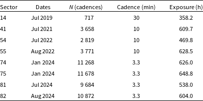
We rejected all cadences with non-zero TESS QUALITY flags. Instrumental systematics were corrected using the Pixel Level Decorrelation (PLD) method implemented in the lightkurve package (Lightkurve Collaboration 2018). We applied a second-order PLD correction with 8 PCA components derived from the pixel-level variability. This was followed by a Ridge regression against a design matrix containing the centroid offsets (x, y and their squares), the estimated background, and a second-order time polynomial to remove residual long-term trends. Table 1 summarises the effective sampling per sector after screening.
TESS sampling and effective exposure per sector after instrumental screening. The dates correspond to the month in which observations of each TESS sector began.

Table 1. Long description
The table presents TESS sampling and effective exposure per sector after instrumental screening. It includes data for various sectors, with columns for Sector, Dates, N (cadences), Cadence (min), and Exposure (h). The table has 8 rows and 5 columns. Column headers are Sector, Dates, N (cadences), Cadence (min), and Exposure (h). Row-wise data: Row 1: Sector 14, Dates Jul 2019, N (cadences) 717, Cadence (min) 30, Exposure (h) 358.2. Row 2: Sector 41, Dates Jul 2021, N (cadences) 3658, Cadence (min) 10, Exposure (h) 609.7. Row 3: Sector 54, Dates Jul 2022, N (cadences) 2819, Cadence (min) 10, Exposure (h) 469.8. Row 4: Sector 55, Dates Aug 2022, N (cadences) 3771, Cadence (min) 10, Exposure (h) 628.5. Row 5: Sector 74, Dates Jan 2024, N (cadences) 11268, Cadence (min) 3.3, Exposure (h) 626.0. Row 6: Sector 75, Dates Jan 2024, N (cadences) 11678, Cadence (min) 3.3, Exposure (h) 648.8. Row 7: Sector 81, Dates Jul 2024, N (cadences) 9684, Cadence (min) 3.3, Exposure (h) 538.0. Row 8: Sector 82, Dates Aug 2024, N (cadences) 10872, Cadence (min) 3.3, Exposure (h) 604.0.
For context we also retrieved the 15–50 keV Swift/BAT daily light curve from the public Transient MonitorFootnote 1 (Krimm et al. Reference Krimm2013) to mark epochs of enhanced high-energy activity. We use the BAT light curve only as a qualitative tracer of the long-term hard-X-ray state. Because the source spectrum changes between faint and bright states, we do not apply a single BAT count-rate-to-bolometric-flux conversion across the full baseline; instead, the representative luminosities discussed below are tied to published pointed spectral analyses.
3. Results
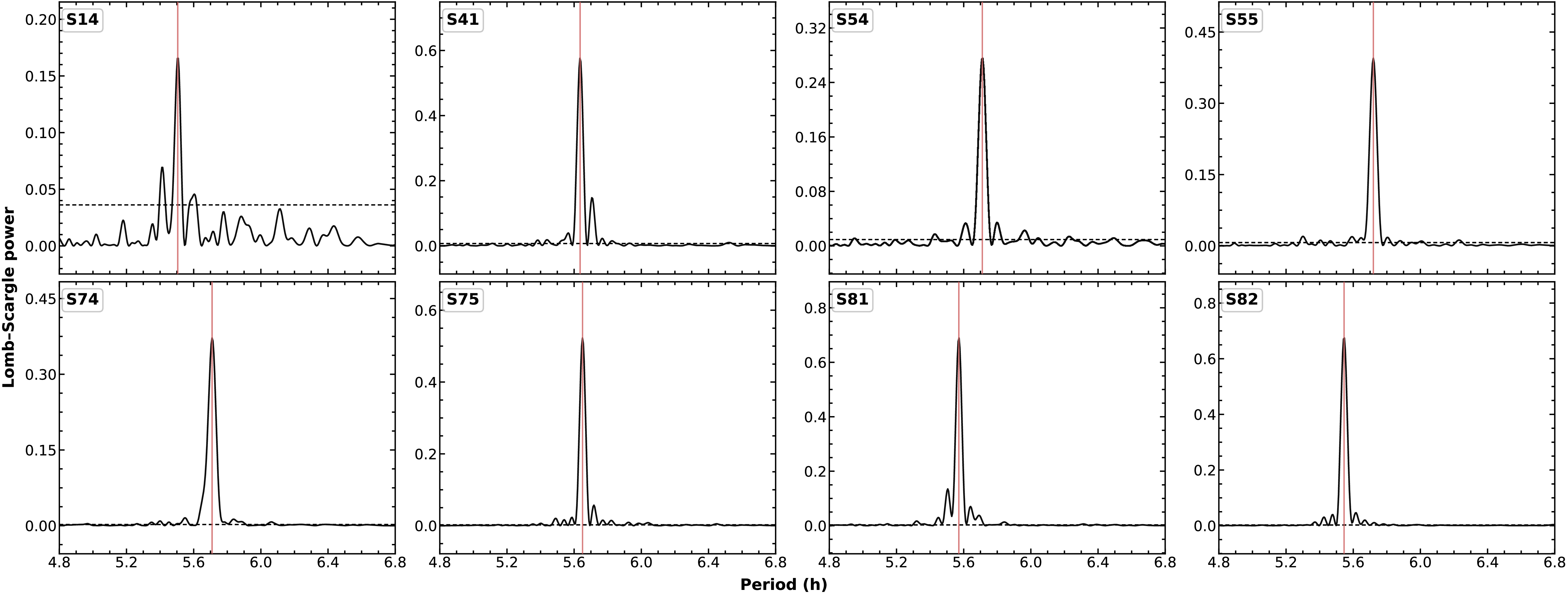
To retain hour-scale power while suppressing slow instrumental and astrophysical trends, we applied a locally weighted regression (LOESS; Cleveland Reference Cleveland1979) high-pass filter with a 0.75 d window, which is large compared to the spin period but small enough to remove day-scale drifts. We then computed Generalised Lomb–Scargle (GLS) periodograms over the 2–10 h trial-period range on dense frequency grids (Scargle Reference Scargle1982; Zechmeister & Kürster Reference Zechmeister and Kürster2009; VanderPlas Reference VanderPlas2018). The dominant peak in each sector was modelled directly in period space with a Gaussian; the fitted mean and standard deviation yielded the sector period and an initial uncertainty. The resulting GLS periodograms for all sectors are shown in Figure 1. Under a white Gaussian-noise null hypothesis, the dominant peaks in all sectors exceed the
 $5\sigma$
false-alarm threshold computed with astropy (Astropy Collaboration et al. 2022).
GLS periodograms by sector (2–10 h). Curves show power in standard normalisation; vertical markers indicate the Gaussian-fitted peak. The
 $5\sigma$
FAP threshold is shown for reference.

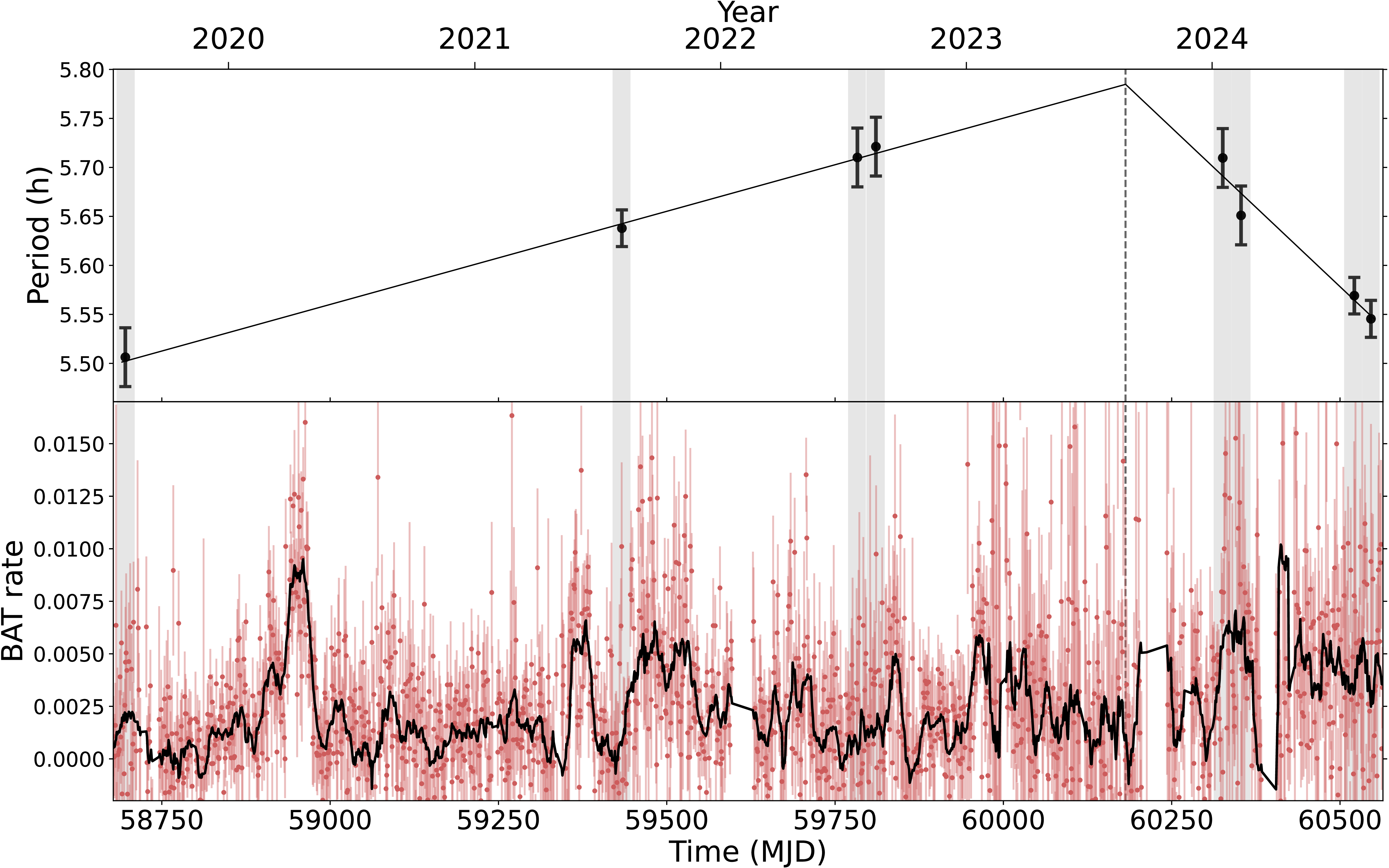
Top: Evolution of the best optical period of 4U 1954+319 across the TESS baseline. Points are sector values (1
 $\sigma$
bars). Grey bands mark each visit. The solid line is the BIC-selected piecewise-linear fit with a mid–2023 break. Bottom: Swift/BAT 15–50 keV daily light curve (Krimm et al. Reference Krimm2013) with TESS visits (grey bands); the solid black curve shows a 15-day running mean BAT light curve. The optical torque reversal occurs between the 2022 and 2024 visits, during relatively modest hard X-ray activity in the Swift/BAT monitor, with no clear contemporaneous outburst comparable to the brighter X-ray episodes reported in pointed observations.

Because red noise can bias false-alarm probabilities (FAPs), we modelled the high-pass residuals in each sector as a stationary Ornstein–Uhlenbeck (OU) process plus a white-noise floor (see e.g. Kelly et al. Reference Kelly, Bechtold and Siemiginowska2009, Reference Kelly, Becker, Sobolewska, Siemiginowska and Uttley2014). For each sector we estimated the OU correlation time
 $\tau$
by fitting the autocorrelation function of the residuals and then generated
 $2\times10^4$
OU+white surrogate light curves at the native cadence. We recomputed the GLS periodogram for each surrogate and obtained Laplace-corrected FAPs,
 $(k{+}1)/(N{+}1)$
(Jaynes Reference Jaynes2003; Vaughan Reference Vaughan2005). All sectors reached the Monte Carlo floor (
 $\mathrm{FAP}\lesssim 5\times10^{-5}$
) both locally and globally across the scanned band. The median OU correlation time across sectors is
 $\tilde{\tau}\approx0.18$
d (
 ${\sim}$
260 min), shorter but comparable to the spin timescale. We therefore consider it unlikely that red noise alone can reproduce a coherent 5–6 h pulsation of the kind observed here.
As an additional robustness check, we repeated the GLS search with
 $n_\mathrm{terms}=2$
and 3 to account for the mild asymmetry seen in some pulse profiles. In all sectors, the multi-harmonic solutions increased the peak power but changed the best-fit periods only slightly, typically at the level of
 ${\sim}1$
s and by at most
 ${\sim}2.7$
s, leaving the secular period evolution and the inferred torque reversal unchanged. We therefore retain the single-harmonic GLS as the reference analysis for consistency with the red-noise validation pipeline. The sector-to-sector harmonic content introduces only a small model-dependent systematic in the recovered periods, negligible compared with the full amplitude of the secular evolution across the TESS baseline.
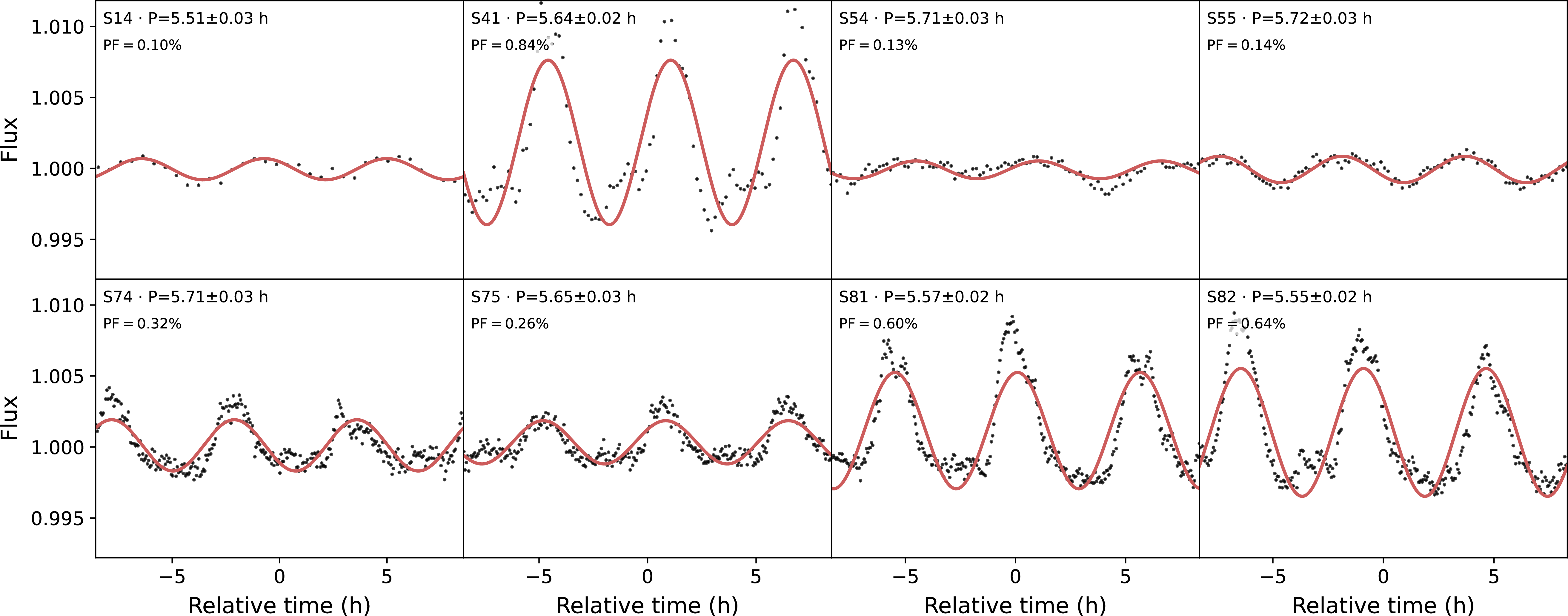
TESS light curves by sector (two cycles shown). Profiles use each sector’s best period.

Figure 3. Long description
Eight line graphs depict flux over relative time for different sectors. Each graph represents data from a specific sector, labeled as S14, S41, S54, S55, S74, S75, S81, and S82. The x-axis of each graph is labeled Relative time (h), ranging from -5 to 5 hours. The y-axis is labeled Flux, ranging from 0.995 to 1.010. Each graph shows a red line representing the best-fit period for the sector, with black dots indicating data points. The periods and false alarm probabilities (PF) for each sector are as follows: S14 with a period of 5.51 plus or minus 0.03 hours and PF of 0.10 percent, S41 with a period of 5.64 plus or minus 0.02 hours and PF of 0.84 percent, S54 with a period of 5.71 plus or minus 0.03 hours and PF of 0.13 percent, S55 with a period of 5.72 plus or minus 0.03 hours and PF of 0.14 percent, S74 with a period of 5.71 plus or minus 0.03 hours and PF of 0.32 percent, S75 with a period of 5.65 plus or minus 0.03 hours and PF of 0.26 percent, S81 with a period of 5.57 plus or minus 0.02 hours and PF of 0.60 percent, and S82 with a period of 5.55 plus or minus 0.02 hours and PF of 0.64 percent. The graphs show periodic variations in flux for each sector, with the red lines fitting the data points to illustrate the periodic trends.
To propagate red noise into the period uncertainties, we performed
 $10^3$
injections per sector of the best-fit sinusoid into OU+white surrogate light curves and re-fitted the local GLS peak in a narrow window around the true period. The resulting distribution of recovered periods yields a red-noise-dominated uncertainty
 $\sigma_{P,\mathrm{red}}\approx(5$
–
 $7)\times10^{-2}$
h, that is, about 1% of P and roughly three times the Gaussian width from the single-peak fit.
Figure 2 shows the sector-by-sector periods, which evolve non-monotonically: an increase from
 $5.51\pm0.06$
h (2019) to
 $5.72\pm0.06$
h (2022), followed by a decrease to
 $5.55\pm0.05$
h by late 2024. To estimate the slopes and the break time, we modelled the period evolution P(t) with a piecewise-linear function sampled with a Markov Chain Monte Carlo ensemble sampler. This provides an empirical description of the secular trend over the available baseline. The analysis yields a reference period of
 $P_\mathrm{ref} = 5.76 \pm 0.02$
h and characterises the evolution as an initial spin-down phase with
 $\dot P_1 = +0.68 \pm 0.08$
s d
 $^{-1}$
, followed by a torque reversal to a spin-up of
 $\dot P_2 = -2.16 \pm 0.35$
s d
 $^{-1}$
. The transition time is constrained to
 $t_\mathrm{br} = 60163^{+43}_{-49}$
MJD.
For pulse-profile characterisation, each sector was folded on its own best period using the common epoch
 $T_0 [\mathrm{MJD}] = 58\,696.2744$
, phases on [0, 2), and median bins of width
 $\Delta\phi = 0.05$
, see Figure 3. We quantify the modulation with the peak-to-peak pulsed fraction, defined as:
 \begin{equation} \mathrm{PF} = \frac{f_{\max}-f_{\min}}{f_{\max}+f_{\min}},\end{equation}
and quoted in percent throughout; with this definition, PF ranges from
 $0.10\%$
to
 $0.84\%$
across sectors. We do not interpret the absolute phase of the profile maximum, since each sector is folded with its own best period while keeping a common reference epoch. We therefore use Figure 3 mainly to compare the pulse-profile morphology.
We have also searched for intrasector changes of the spin period by computing the GLS periodogram on a five-days, 50% overlapping window during each sector, while the error in the period was determined using the same method described above for the analysis of the full sector periodograms. To assess whether the detected intrasector period variations represent physical spin-evolution trends or are dominated by stochastic flickering, we applied the Wald-Wolfowitz runs test to the period measurements of each TESS sector. The resulting p-values (ranging from
 $0.10$
to
 $0.72$
) consistently exceed the
 $\alpha = 0.05$
significance threshold. This indicates that the null hypothesis of a random distribution cannot be rejected, confirming that there is no statistically significant linear or monotonic trend within individual sectors. Consequently, the long-term torque reversal observed in mid-2023 must be interpreted as the result of inter-sector evolution.
4. Discussion
The TESS data reveal coherent optical pulsations from 4U 1954+319 over a five-year baseline, with periods drifting between
 ${\sim}$
5.5 and
 ${\sim}$
5.7 h and sector-to-sector pulsed fractions of
 ${\sim}0.1$
–1%. The timing behaviour is consistent with a change in slope around mid–2023, corresponding to a torque reversal from spin-down to stronger spin-up. The reversal occurs during a period of modest BAT activity. There is no indication of a major hard-X-ray state change or a persistent disc-fed state during the TESS coverage. Although temporary disc formation during brighter outbursts cannot be excluded, the 2022–2024 interval sampled by TESS does not show clear evidence for such a state. We further note that brighter X-ray episodes reported at other epochs, such as the 2012 event discussed by Enoto et al. (Reference Enoto2014), likely probe a distinct and brighter accretion regime from the one sampled here.
The optical amplitudes are much smaller than the 60–80% X-ray pulsed fractions measured during outbursts (Enoto et al. Reference Enoto2014). This points to reprocessing of the pulsed high-energy beam as the likely origin of the optical modulation. The observed
 ${\sim}0.1$
–1% pulsed fractions could arise from reprocessing in small-covering-fraction regions: the magnetospheric surroundings and base of the accretion flow, the inner, partially ionised donor wind, or a restricted irradiated patch on the M-supergiant photosphere (e.g. Charles & Coe Reference Charles, Coe, Lewin and van der Klis2006; Luna Reference Luna2023). Dilution by the luminous M supergiant can also account for the small amplitudes and for part of their sector-to-sector variability. Under this interpretation, the optical pulsations provide an indirect but coherent tracer of the spin modulation of the accretion flow, while the secular evolution of the pulsation period traces the net torque on the NS.
4.1. Torque balance and (near-)equilibrium spin
We adopt
 $N\gt0$
for spin-up and write the accretion torque as
 \begin{equation}N \;=\; 2\pi I\,\dot{\nu} \;=\; -\,\frac{2\pi I}{P^{2}}\,\dot P,\end{equation}
with
 $I=10^{45}$
g cm
 $^{2}$
. For a representative
 $P=5.76$
h (
 $2.07\times10^{4}$
s), the pre-break spin-down rate
 $\dot P_1=+0.68\pm0.08$
s d
 $^{-1}$
corresponds to
 $N_1\approx(\!-\!1.2\pm0.1)\times10^{32}$
dyn cm, while the post-break spin-up
 $\dot P_2=-2.16\pm0.35$
s d
 $^{-1}$
corresponds to
 $N_2\approx$
 $(\!+\!3.6\pm0.6)\times10^{32}$
dyn cm. The corresponding spin-down power
 \begin{equation}L_\mathrm{sd} = 4\pi^{2} I \frac{|\kern1.5pt\dot{\!P}|}{P^{3}}\end{equation}
is
 ${\sim}10^{29}$
erg s
 $^{-1}$
for the measured P and
 $\dot P$
, several orders of magnitude below the X-ray luminosity. The spin evolution is therefore governed by angular-momentum exchange with the accretion flow, not by a spin-powered outflow.
The measured fractional rates,
 $(\dot P/P)\simeq +1.2\%$
yr
 $^{-1}$
before the break and
 $-3.8\%$
yr
 $^{-1}$
afterwards, imply that on year-long timescales the star can move noticeably away from and back towards a torque-balanced state. Over a decade, a steady spin-up at the observed post-break rate would reduce the period by
 ${\sim}38\%$
, inconsistent with the long-term behaviour seen in X-rays (Corbet et al. Reference Corbet, Sokoloski, Mukai, Markwardt and Tueller2008; Enoto et al. Reference Enoto2014). The torque reversal identified here therefore fits into a scenario in which 4U 1954+319 undergoes a sequence of spin-up and spin-down episodes of comparable magnitude, such that the long-term average torque remains small and the star resides near a quasi-equilibrium spin period determined by the wind-fed accretion flow.
4.2. Settling accretion and the magnetic field
Within the quasi-spherical settling accretion framework (Shakura et al. Reference Shakura, Postnov, Kochetkova and Hjalmarsdotter2012, Reference Shakura, Postnov, Kochetkova and Hjalmarsdotter2014; Shakura & Postnov Reference Shakura and Postnov2017), the Alfvén radius scales as
 \begin{equation}R_\mathrm{A}\simeq 1.5\times10^{9}\,\mu_{30}^{6/11}\,\,\dot{\!M}_{16}^{-2/11}\ \mathrm{cm},\end{equation}
where
 $\mu_{30}$
is the dipole moment in units of
 $10^{30}$
G cm
 $^{3}$
and
 $\dot M_{16}$
is the mass accretion rate in units of
 $10^{16}$
g s
 $^{-1}$
. The characteristic torque can be written as
 \begin{equation}N\,\sim\,\dot M\sqrt{GM_\ast R_\mathrm{A}} \propto\, \dot{\!M}^{10/11}\,\mu^{3/11},\end{equation}
so that the torque depends only weakly on both
 $\dot M$
and
 $\mu$
. On that basis, the observed torque ratio
 $\left|N_2/N_1\right|\approx 3.2$
can be reproduced with
 \begin{equation}\frac{\dot M_2}{\dot M_1}\simeq \left|\frac{N_2}{N_1}\right|^{11/10}\approx 3.6.\end{equation}
Accordingly, the observed transition can be explained by a moderate change in the mass accretion rate, without invoking a major restructuring of the flow. Variations in the sign and magnitude of the specific angular momentum carried by the wind may still contribute to the detailed torque balance. Adopting a representative low-state luminosity inferred from the low states analysed by Enoto et al. (Reference Enoto2014),
 \begin{equation}L_X \simeq 3\times10^{34}\left(\frac{d}{1.7\,\mathrm{kpc}}\right)^2\ \mathrm{erg\ s^{-1}},\end{equation}
the Gaia-based distance of Hinkle et al. (Reference Hinkle2020),
 $d \simeq 3.3\,\mathrm{kpc}$
, implies
 $L_X \simeq 1.1\times10^{35}\ \mathrm{erg\ s^{-1}}$
and hence
 \begin{equation}\dot M \simeq \frac{L_X R_\ast}{G M_\ast}\simeq 1.6\times10^{14}\left(\frac{d}{1.7\,\mathrm{kpc}}\right)^2\ \mathrm{g\ s^{-1}}\simeq 6.0\times10^{14}\ \mathrm{g\ s^{-1}},\end{equation}
for
 $M_\ast=1.4\,{\rm M}_\odot$
and
 $R_\ast=10^{6}$
cm. Although the torque analysis implies a factor-of-few increase in mass accretion rate after the break, the sector-averaged TESS flux shows no associated brightening. This is consistent with the optical continuum being dominated by the M-supergiant photosphere, for which
 $L_\mathrm{opt} \sim 10^{38}$
erg s
 $^{-1}$
(Hinkle et al. Reference Hinkle2020), compared with an accretion luminosity of order
 $L_\mathrm{acc}\sim10^{35}$
erg s
 $^{-1}$
in representative low states on the Gaia distance scale. A factor-of-few change in the accretion flow would therefore not necessarily produce a detectable change in the spin-averaged optical light curve.
For a dipole moment
 $\mu_{30}\sim1$
(
 $B\sim10^{12}$
G) this gives
 $R_\mathrm{A}\approx 3\times10^{9}$
cm and a characteristic torque
 $N\approx 1\times10^{32}$
dyn cm, increasing to
 ${\sim}3.6\times10^{32}$
dyn cm when
 $\dot M$
is raised by a factor of
 ${\sim}3.6$
. Both values match, to within factors of order unity, the torques inferred from the observed
 $\dot P$
. Allowing for uncertainties in
 $L_X$
, geometry, and the settling-accretion scalings, the torque amplitude and its dependence on
 $\dot M$
are consistent with a surface dipole field in the range
 $B\approx (0.5$
–
 $5)\times10^{12}$
G.
For
 $P=5.76$
h the co-rotation radius is
 \begin{equation}R_\mathrm{co}=\left(\frac{GM_\ast P^{2}}{4\pi^{2}}\right)^{1/3}\approx 1.2\times10^{11}\ \mathrm{cm},\end{equation}
so that
 $R_\mathrm{A}\ll R_\mathrm{co}$
across the TESS baseline. The magnetosphere therefore remains well inside co-rotation, far from the centrifugal-inhibition condition
 $R_\mathrm{A}\approx R_\mathrm{co}$
required for a transition to a strong propeller. Magnetic or centrifugal gating models in which
 $R_\mathrm{A}\sim R_\mathrm{co}$
predict abrupt, correlated changes in X-ray flux and spectral hardness as the torque switches sign (Bozzo et al. Reference Bozzo, Falanga and Stella2008). We do not find clear evidence for such behaviour in the contemporaneous Swift/BAT monitoring, which shows only modest variability around the torque reversal. By contrast, brighter X-ray episodes reported at other epochs, such as the 2012 outburst (Enoto et al. Reference Enoto2014), likely probe a different accretion regime from the one sampled during the TESS baseline and may be associated with stronger spin-up phases.
The same scaling can be inverted to estimate the field strength needed to bring the magnetosphere close to
 $R_\mathrm{A}\approx R_\mathrm{co}$
at the observed
 $\dot M$
. Keeping
 $\dot M$
fixed and using
 $R_\mathrm{A}\propto \mu^{6/11}$
, raising
 $R_\mathrm{A}$
from
 $3\times10^{9}$
to
 $1.2\times10^{11}$
cm would require an increase in dipole moment by a factor
 $\sim(40)^{11/6}\approx 9\times10^{2}$
, corresponding to
 $B\sim 10^{15}$
G. This is well above the field range needed to match the observed torque scale and is not favoured by the absence of clear propeller episodes. A long-lived Keplerian disc is also not required by the data: for the inferred
 $\dot M$
and B, standard disc-torque prescriptions (see e.g. Ghosh & Lamb Reference Ghosh and Lamb1979a,b) would tend to give spin-up torques larger than observed unless the system were very close to torque equilibrium.
Our interpretation is complementary to the source-specific reanalysis of 4U 1954+319 by Bozzo et al. (Reference Bozzo, Ferrigno, Oskinova and Ducci2022a), who revisited the system in light of the revised donor properties and the Gaia-based distance. Their results highlight how the updated system parameters affect both the inferred accretion geometry and the magnetic-field constraints derived from the spin evolution. In this context, the torque reversal measured here provides an additional empirical constraint on the sign and amplitude of the torque for future source-specific modelling.
4.3. Period variability and torque noise
A purely kinematic (Doppler) origin for the observed reversal in P is strongly disfavoured by the implied radial-velocity amplitude. Interpreting the period variation (
 $5.51 \to 5.72 \to 5.55$
h) as a line-of-sight velocity modulation would require a fractional amplitude
 $\Delta P/P\sim0.04$
. The corresponding radial-velocity amplitude,
 \begin{equation}v_r \simeq c\,\frac{\Delta P}{P},\end{equation}
would be of order
 $1.2\times10^{4}$
km s
 $^{-1}$
, far above the velocities expected for a wind-fed system of this type. The measured period evolution is therefore most naturally interpreted as reflecting intrinsic changes in the neutron-star spin.
Accreting pulsars generically exhibit red torque noise, with power spectra often consistent with random walks in spin frequency
 $\nu$
or its derivative
 $\dot{\nu}$
on long timescales (Deeter & Boynton Reference Deeter and Boynton1982; Bildsten et al. Reference Bildsten1997). In the settling-accretion scenario, stochastic fluctuations in the specific angular momentum of the captured wind, combined with the dynamics of the convective shell above the magnetosphere, both modulate the torque (Shakura & Postnov Reference Shakura and Postnov2017). The sector-to-sector changes in optical pulsed fraction (
 ${\sim}0.1$
–1%) and the sign-changing, intermediate-strength torques observed here are consistent with stochastic angular-momentum exchange in a wind-fed accretion flow. In this interpretation, fluctuations in the captured wind and in the quasi-spherical shell can modulate the torque without requiring a persistent disc or a propeller transition (Shakura & Postnov Reference Shakura and Postnov2017). The characteristic correlation time of the noise in the TESS light curves,
 $\tau\sim0.2$
d, is shorter than but comparable to the spin period and to the dynamical time at radii
 ${\sim}10^{11}$
cm, close to the co-rotation radius. This does not establish a one-to-one causal link. It only shows that the optical red noise and the torque fluctuations occur on timescales compatible with large-scale variability in the wind-fed flow.
4.4. Comparison with other X-ray binaries
Although 4U 1954+319 is now classified as a HMXB with an M-type red supergiant donor (Hinkle et al. Reference Hinkle2020; Fortin et al. Reference Fortin2023; Neumann et al. Reference Neumann, Avakyan, Doroshenko and Santangelo2023), its spin behaviour is similar in some respects to that of SyXBs in the settling-accretion regime. GX 1+4 is the prototypical example, with extended intervals of alternating spin-up and spin-down and only modest, correlated changes in X-ray flux (e.g. González-Galán et al. Reference González-Galán2012; Ilkiewicz et al. Reference Iłkiewicz, Mikołajewska and Monard2017; Serim et al. Reference Serim, Şahiner, Çerri-Serim, İnam and Baykal2017). Its long-term evolution is interpreted as that of a NS accreting from a slow, structured giant wind and fluctuating around a torque-balanced state. 4U 1954+319 occupies a similar low-luminosity regime but at much longer spin periods and with torques of order
 $N\sim10^{32}$
dyn cm, well below the values reached during its bright X-ray spin-up episodes (Enoto et al. Reference Enoto2014; Corbet et al. Reference Corbet, Sokoloski, Mukai, Markwardt and Tueller2008). The sequence of spin-down followed by stronger spin-up, with comparable amplitudes and a small net torque over several years, is consistent with the generic expectations of quasi-spherical settling accretion, where moderate variations in
 $\dot M$
and in the specific angular momentum of the wind can drive torque reversals around an equilibrium period (e.g. Shakura et al. Reference Shakura, Postnov, Kochetkova and Hjalmarsdotter2012; Shakura et al. Reference Shakura, Postnov and Hjalmarsdotter2013; Shakura & Postnov Reference Shakura and Postnov2017; Yungelson et al. Reference Yungelson, Kuranov and Postnov2019; Mao et al. Reference Mao2024). Other symbiotic candidates such as 4U 1700+24 and Sct X-1, although lacking a secure spin period determination, are likewise interpreted as wind-fed systems with strongly magnetised NSs at low X-ray luminosities (Masetti et al. Reference Masetti, Orlandini, Palazzi, Amati and Frontera2006; Corbet et al. Reference Corbet, Sokoloski, Mukai, Markwardt and Tueller2008; Bozzo et al. Reference Bozzo, Romano, Ferrigno and Oskinova2022b). This suggests that 4U 1954+319 may sample a broader class of low-luminosity, wind-fed systems.
A similar torque phenomenology is seen in several classical wind-fed HMXBs with OB supergiant donors. Sources such as Vela X
 $-$
1, 4U 1538
 $-$
52, and GX 301
 $-$
2 show strong torque noise that is statistically consistent with fluctuations driven by an inhomogeneous stellar wind (Bildsten et al. Reference Bildsten1997; Serim et al. Reference Serim, Serim and Baykal2023). The supergiant system 4U 1907+09 is a particularly close analogue: it undergoes long intervals of spin-down punctuated by transitions to spin-up, with spin derivatives of comparable magnitude and only moderate changes in luminosity (Fritz et al. Reference Fritz2006; Inam et al. Reference Inam, Şahiner and Baykal2009). Vela X
 $-$
1 also shows alternating spin-up and spin-down on timescales of tens of days, with typical hard X-ray flux variations of only a factor
 ${\sim}$
1.5–2 between different torque states (e.g. Martínez-Núñez et al. Reference Martínez-Núñez2017; Serim et al. Reference Serim, Serim and Baykal2023). In these systems, torque reversals and timing noise are usually linked to stochastic changes in
 $\dot M$
and in the angular momentum of the captured wind. A persistent Keplerian disc or a strong propeller transition is not required. The torques measured in 4U 1954+319, their amplitudes, and their sign changes are consistent with this wind-fed scenario, but at lower
 $L_X$
and at much longer
 $P_\mathrm{s}$
, extending the parameter space over which such behaviour is observed.
An observational comparison can also be made with transitional millisecond pulsars, in which coherent optical pulsations have likewise been detected while their physical origin remains debated (Ambrosino et al. Reference Ambrosino2017; Papitto et al. Reference Papitto2019; Illiano et al. Reference Illiano2023). In those systems, the optical pulsations are unexpectedly strong relative to the X-ray pulsations and have been discussed in terms of magnetospheric emission, synchrotron radiation, or accretion-related processes close to the NS. Although 4U 1954+319 differs substantially in spin period, donor type, accretion geometry, and magnetic-field regime, both cases indicate that optical timing can reveal coherent pulsations and long-term spin behaviour even when the high-energy phenomenology alone does not uniquely determine the emission mechanism.
Here the timing solution comes from the optical data. The X-ray monitoring provides context, but it does not define the spin evolution. This shows that reprocessed optical pulsations can be used to follow the spin of a wind-fed accreting pulsar in a relatively faint X-ray state. The same approach may work for other long-period wind-fed systems, especially those with spin periods of a few hours to a day and optical pulsed fractions of
 ${\sim}0.1$
–a few per cent. SyXBs and long-period HMXBs are good candidates because their slow spins match the cadence and baseline of all-sky optical surveys such as TESS and, in the future, PLATO (Rauer et al. Reference Rauer2014). Optical timing can complement sparse X-ray coverage and provide an additional way to monitor torque noise in wind-fed accreting pulsars. Optical timing can therefore complement sparse X-ray coverage by providing an additional way to monitor torques and torque noise in wind-fed accreting pulsars.
Acknowledgement
EAS acknowledges support by the Spanish Agencia estatal de investigación via PID2021-124879NB-I00 and PID2024-161863NB-I00. GJML is member of the CIC-CONICET (Argentina).
Data availability statement
The TESS light curves used in this work are publicly available from the Mikulski Archive for Space Telescopes (MAST).
 5σ
 σ

 Open access

