1 Introduction
The description of the wave field in the near shore region is one of the most important aspects of marine engineering. This is where most of the human interactions with the sea occur. Waves in this zone have an impact on shipping, sediment transport, offshore and coastal construction and the extraction of wave energy. Current operational forecasting models are not able to accurately predict the wave evolution in shallow to intermediate water, in part due to the inability to accurately account for triad interactions. The errors are not solely in magnitude as, due to the nonlinear interactions, new directional wave harmonics are generated.
Operational models are used to predict the large-scale evolution of the wave field. Some of the most commonly used ones are WAVEWATCH III by Tolman (Reference Tolman2009), WAM by WAMDI group (1988) and SWAN by Holthuijsen, Booij & Ris (Reference Holthuijsen, Booij and Ris1993). They are based on the wave action equation (WAE). There are several ways to define the WAE: the one in Cartesian coordinates for bathymetries with parallel bottom contours is defined as
 $$\begin{eqnarray}\displaystyle {\displaystyle \frac{\unicode[STIX]{x2202}{\mathcal{A}}_{p,l}}{\unicode[STIX]{x2202}t}}+\unicode[STIX]{x1D735}\boldsymbol{\cdot }(\overrightarrow{C}_{g,p}{\mathcal{A}}_{p,l})=S_{TOT,p,l}. & & \displaystyle\end{eqnarray}$$
Here,
 $S_{TOT,p,l}$
is the sum of various source terms, and
 ${\mathcal{A}}_{p,l}$
is the wave action defined as
 $$\begin{eqnarray}\displaystyle {\mathcal{A}}_{p,l}={\displaystyle \frac{\langle |a_{p,l}|^{2}\rangle }{\unicode[STIX]{x1D714}_{p}}}, & & \displaystyle\end{eqnarray}$$
where
 $a$
is the complex amplitude,
 $l$
denotes the lateral wavenumber index and
 $\unicode[STIX]{x1D714}_{p}=\unicode[STIX]{x1D714}_{min}p$
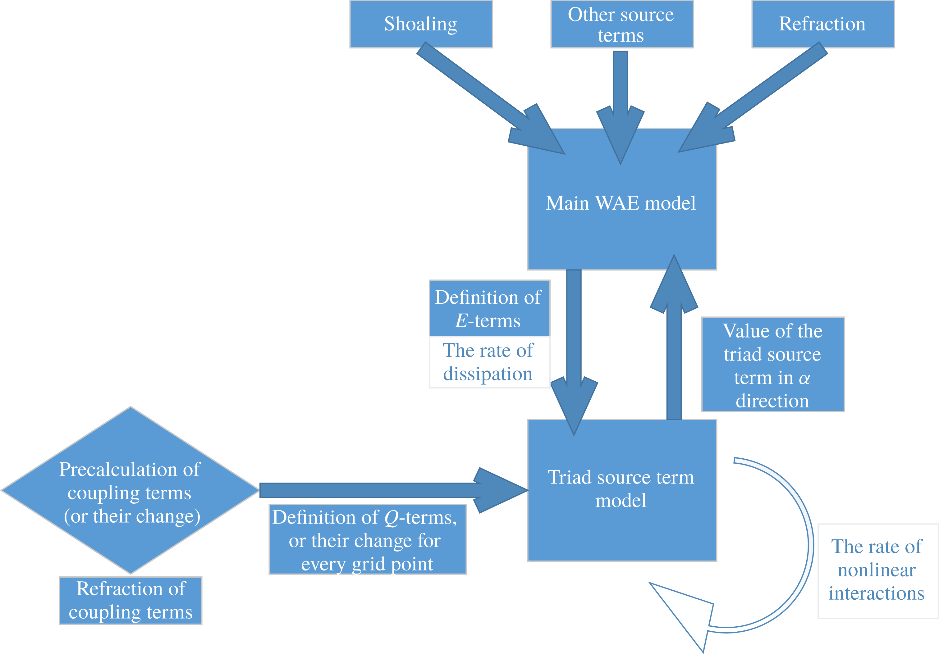
is the angular frequency. The left-hand side of (1.1) is the linear part of the WAE which describes changes of the wave action in time and space. The WAE is often used for large-scale simulation of wave evolution in coastal areas. Wave evolution in these areas is mostly determined by the triad source term, and the breaking term. However, the existing triad source term formulations (lumped triad approximation (LTA) – Eldeberky & Battjes (Reference Eldeberky, Battjes, Dally and Zeidler1995), stochastic parametric model based on Boussinesq equations (SPB) – Becq-Girard, Forget & Benoit (Reference Becq-Girard, Forget and Benoit1999), consistent collinear triad approximation (CCA) – Salmon et al. (Reference Salmon, Smit, Janssen and Holthuijsen2016)) are one-dimensional (1-D) in nature, and cannot account for the full two-dimensional (2-D) properties of the wave field. Another approach is to solve Reynolds-averaged Navier–Stokes equations (e.g. SWASH model, Zijlema, Stelling & Smit (Reference Zijlema, Stelling and Smit2012)). This approach already simulates 2-D wave shoaling, but as it is far more computationally intensive it is typically used for smaller scale wave evolution such as for harbours. One of the main goals of this work is the derivation of a model for the nonlinear triad source term suitable for implementation into operational wave models.
Recently there has been a significant development of 2-D stochastic nonlinear wave models in shallow water, including Janssen (Reference Janssen2009), which follows a Hamiltonian approach, quasi-two-dimensional mild slope models such as Kofoed-Hansen & Rasmussen (Reference Kofoed-Hansen and Rasmussen1998), Eldeberky & Madsen (Reference Eldeberky and Madsen1999), Agnon & Sheremet (Reference Agnon and Sheremet2000); Boussinesq models from Herbers & Burton (Reference Herbers and Burton1997); and fully 2-D models derived in Kaihatu & Kirby (Reference Kaihatu and Kirby1995). There are other localized models such as Becq-Girard et al. (Reference Becq-Girard, Forget and Benoit1999), Stiassnie & Drimer (Reference Stiassnie and Drimer2006), Toledo & Agnon (Reference Toledo and Agnon2012). In the work of Smit & Janssen (Reference Smit and Janssen2013) and Smit, Janssen & Herbers (Reference Smit, Janssen and Herbers2015) a new type of model was derived by expanding the wave field in wavenumber space, while also propagating information on the wave phasings.
Wave breaking is, together with triad interactions, a dominant source term in the breaking zone and needs to be accounted for. Several models for the breaking source term, based on the work of Battjes & Janssen (Reference Battjes and Janssen1978), are considered. First, a total energy dissipation is calculated and then it is distributed across the harmonics either as frequency dependent (as done in Mase & Kirby (Reference Mase and Kirby1992)), or with a uniform distribution (as done in Eldeberky & Battjes (Reference Eldeberky and Battjes1996)). Both approaches were tested and found to work to the leading order, however, there were certain discrepancies. It is speculated by the authors that the empirical model for wave breaking also takes into account other effects, such as triad interactions and turbulence, which make them unsuitable for a more detailed description of the wave field evolution. However, in depth investigation of wave breaking is outside the scope of this work, it is simply noted that it is a complex phenomena.
In Vrecica & Toledo (Reference Vrecica and Toledo2016), following the approach of Stiassnie & Drimer (Reference Stiassnie and Drimer2006) and Toledo & Agnon (Reference Toledo and Agnon2012), a new localized formulation of the stochastic evolution equations has been derived allowing for a consistently accurate representation of the nonlinear shoaling coefficients from deep to shallow water. It showed good agreement with other theoretical models and with experimental data for the case of unidirectional wave propagation with no wave breaking. In this paper the model is extended to the breaking zone, and a method to apply this model as a 2-D
 $S_{nl3}$
source term for phase averaged forecasting models is presented.
The achievements of this paper include a better understanding of wave shoaling and the derivation of a localized 2-D source term for nonlinear triad interactions, fitting for implementation into wave forecasting models (e.g. WAVEWATCH III). The most important feature of the model is its ability to accurately describe wave evolution both from deep water to the breaking zone. To this end, various improvements to the model of Vrecica & Toledo (Reference Vrecica and Toledo2016) are derived. First-order spatial derivatives and dissipation effects are incorporated into the nonlinear interaction coefficient of Bredmose et al. (Reference Bredmose, Agnon, Madsen and Schaffer2005), greatly increasing its accuracy in the breaking zone. The newly defined deterministic model is used to derive a new formulation of the stochastic model, which is consistent from deep to breaking waters. In Agnon & Sheremet (Reference Agnon and Sheremet2000), Stiassnie & Drimer (Reference Stiassnie and Drimer2006), Toledo & Agnon (Reference Toledo and Agnon2012), Vrecica & Toledo (Reference Vrecica and Toledo2016) it was assumed that spectrum components in the integral of the bispectrum evolution equation are nearly constant, and they were taken out of it. In the consistent from deep to breaking waters (CDB) model, those changes are accounted for, either by approximate solutions of spectrum components, or by more accurate solutions obtained through iterations.
The present formulations of both deterministic and stochastic models do not account for four wave interactions. While it is a straightforward procedure to include them, as the goal of this work is to provide insight on triad interactions, it was decided not to consider four wave interactions. This means that the presented models, on their own, are not applicable in deep water and over long stretches of intermediate water (order of (
 $k^{-1}\unicode[STIX]{x1D702}^{-2}$
)). The bottom slope also plays a role as an additional component, as sharp slopes in the intermediate water region can dominate the nonlinear interactions. In the numerical simulations presented in this paper, three wave interactions are the dominant term at the end of propagation.
Another limitation lies in the shallow water limit due to strong nonlinearity and non-dispersiveness of shallow water waves. If dispersion correction
 $(kh)^{2}$
becomes of same order as nonlinearity (
 $a/h$
) the energy will quickly cascade to higher frequencies, and dissipate. Furthermore, coherent wave patterns will form leading to the failure of the standard closure and the inapplicability of the linear dispersion relation. The inclusion of wave slopes in the nonlinear term seems to extend the applicability of the deterministic model, as it accounts for a part of the nonlinear effects in the dispersion relation. It should be possible to account for full nonlinear effects in the dispersion relation by using a similar approach, but with significantly higher numerical costs. Regarding the stochastic model, while the closure of Holloway (Reference Holloway1980) helped somewhat, the model still failed shortly after meeting this criteria. This is, however, an extreme scenario for a stochastic approach and can be a topic for further study.
The stochastic model, if a proper cubic source term is included, can be run in deep and intermediate waters. On the other hand, the deterministic model would need to be augmented with cubic terms in order to be applicable in deep water, where triads would be non-resonant anyway. It would be of interest though to further analyse wave evolution in intermediate waters. In this area both triad and quartet interactions, as well as bottom friction, can be relevant for wave evolution. It is not clear a priori in which range of parameters the standard closure should be applied. As a rule of thumb both models can be used to depths where
 $(kh)^{2}\approx a/h$
. It seems to be possible to further improve the viability of the deterministic model when accounting for wave slopes. To model wave evolution beyond this point an alternative method would need to be used (possibly the Riemann wave approach).
The accuracy of deterministic and stochastic versions of the model is tested, by comparing their output against the measurements of Freilich & Guza (Reference Freilich and Guza1984) and Smith (Reference Smith2004). A good agreement was found in both cases. The directional properties of a shoaling wave field are examined numerically for directionally spread seas. This example shows the importance of accounting for nonlinear interactions of waves propagating in different directions. The evolution of directionally spread sea wave spectra shows interesting directional properties, which are not accounted for by SPB and LTA models (they only account for interactions of co-propagating waves). An examination of nonlinear coefficients shows that the rate of energy transfer is reduced for a wave field propagating at an oblique angle to the onshore direction. While we do not model non-monotonic slopes, it was shown in Vrecica & Toledo (Reference Vrecica and Toledo2016) that the model is capable of grasping them.
In § 2 the deterministic and stochastic models from Vrecica & Toledo (Reference Vrecica and Toledo2016), which are the base for the new formulation, are presented for reference. In § 3 several improvements for the deterministic and stochastic model are derived. In § 4 the evolution of the wave field in two dimensions over a monotone slope with parallel bottom contours is simulated and compared to other models and experimental results. Finally the conclusions and closing considerations are given in § 5.
2 Deterministic and stochastic evolution equations
The mathematical models derived in Vrecica & Toledo (Reference Vrecica and Toledo2016) are based on the assumption that the bathymetry changes along one main direction. This approach is called quasi-two-dimensional approximation. A deterministic formulation and two different versions of a stochastic formulation, one with a localized triad source term and one with a non-local triad source term, were derived. These models are based on the work of Bredmose et al. (Reference Bredmose, Agnon, Madsen and Schaffer2005), with some differences. In Vrecica & Toledo (Reference Vrecica and Toledo2016), the linear source term was included in the boundary conditions. Additionally, slow time effects have been included into the evolution equation, which are not considered in this paper. Finally, while the model of Bredmose et al. (Reference Bredmose, Agnon, Madsen and Schaffer2005) included some additional effects in the lateral direction by averaging the wavenumber in the lateral direction, the model derived in Vrecica & Toledo (Reference Vrecica and Toledo2016) is based solely on the locally defined wavenumbers, with no lateral averaging or non-local integrated coefficients (as in Agnon & Sheremet (Reference Agnon and Sheremet1997)).
The deterministic evolution equation of Vrecica & Toledo (Reference Vrecica and Toledo2016) is
 $$\begin{eqnarray}\displaystyle & & \displaystyle {\displaystyle \frac{1}{C_{g,p}}}{\displaystyle \frac{\unicode[STIX]{x2202}a_{p,l}}{\unicode[STIX]{x2202}t}}+{\displaystyle \frac{\unicode[STIX]{x2202}a_{p,l}}{\unicode[STIX]{x2202}x}}+{\displaystyle \frac{1}{2C_{g,p}}}{\displaystyle \frac{\unicode[STIX]{x2202}C_{g,p}}{\unicode[STIX]{x2202}x}}a_{p,l}-D_{p,l}a_{p,l}\nonumber\\ \displaystyle & & \displaystyle \quad =-\unicode[STIX]{x1D700}\text{i}\mathop{\sum }_{s=p-N}^{N}\mathop{\sum }_{r=max\{l-M,-M\}}^{min\{l+M,M\}}W_{s,p-s,r,l-r}a_{s,r}a_{p-s,l-r}\text{e}^{-\text{i}\int (k_{s,r}^{x}+k_{p-s,l-r}^{x}-k_{p,l}^{x})\,\text{d}x},\end{eqnarray}$$
where
 $D_{p,l}$
represents a linear dissipation term, for brevity
 $C_{g,p}$
is defined here as the onshore group velocity (
 $C_{g,p}^{x}=C_{g,p}=|\overrightarrow{C}_{g,p}|k^{x}/k$
),
 $a_{p,l}$
is the Fourier amplitude of surface elevation,
 $k^{x}$
represents the wavenumber in the direction of bathymetry changes and
 $W_{s,p-s,r,l-r}$
is the nonlinear interaction coefficient. Both the
 $t$
and
 $x$
terms describe the change of wave amplitude on slow time scales compared to the waves’ phase function. It was also assumed that changes in
 $t$
also act on slower time scales than
 $x$
. In this paper, it is assumed that the wave field does not change in time, and all of the
 $\unicode[STIX]{x2202}t_{1}$
terms are discarded. There is no formulation of dissipation term that is fitting for all possible cases, therefore the
 $D$
-term is undefined. Any formulation can be used, depending on the case under consideration.
The first subscript in
 $a_{p,l}$
defines the frequency of the wave as
 $\unicode[STIX]{x1D714}_{p}=p\,\unicode[STIX]{x1D714}$
, where
 $\unicode[STIX]{x1D714}$
is the lowest frequency in consideration. The second subscript
 $l$
defines the lateral wavenumber as
 $k_{l}^{y}=l\,k_{min}^{y}$
, where
 $k_{min}^{y}$
is the smallest value of the lateral wavenumber space used for the discretization. The directional characteristics of the model are described using lateral wavenumbers of the interacting wave components. As can be seen from (2.1), the interacting components in the nonlinear part close the resonance in frequency (
 $\unicode[STIX]{x1D714}_{p}=\unicode[STIX]{x1D714}_{s}+\unicode[STIX]{x1D714}_{p-s}$
) and in lateral wavenumber (
 $k_{l}^{y}=k_{r}^{y}+k_{l-r}^{y}$
) spaces. The wave field is discretized in
 $N$
complex conjugate pairs in frequency space and 2 M bins in lateral wavenumber space.
Refraction effects are accounted for by the model, in the same way as in Agnon & Sheremet (Reference Agnon and Sheremet1997), but in a different manner than usual. Due to the nature of the discretization used (frequency and constant lateral wavenumber), the energy flux is conserved by definition for a unit length of the lateral direction (see also Bredmose et al.
Reference Bredmose, Agnon, Madsen and Schaffer2005). This means there is no linear shift of energy between the discretized wave components. The direction of every wave component is obtained from the ratio of onshore (
 $k_{x}$
) and lateral (
 $k_{y}$
) wavenumbers. As the water depth decreases, the onshore wavenumber increases (while the lateral one remains constant), leading to shift of wave direction towards the shoreline.
The stochastic model is obtained from (2.1) by multiplying it with the complex conjugate of
 $a_{p,l}$
, and adding the result to its complex conjugate, applying the closure of Benney & Saffman (Reference Benney and Saffman1966) and ensemble averaging (see Vrecica & Toledo (Reference Vrecica and Toledo2016) for more details). This process yields
 $$\begin{eqnarray}\displaystyle & & \displaystyle {\displaystyle \frac{\unicode[STIX]{x2202}E_{p,l}}{\unicode[STIX]{x2202}t}}+{\displaystyle \frac{\unicode[STIX]{x2202}}{\unicode[STIX]{x2202}x}}(C_{g,p}E_{p,l})-2D_{p,l}E_{p,l}\nonumber\\ \displaystyle & & \displaystyle \quad =4\mathop{\sum }_{s=p-N}^{N}\mathop{\sum }_{r=max\{l-M,-M\}}^{min\{l+M,M\}}\text{Re}[Q_{s,p-s,r,l-r}+Q_{p,s,l,t-r}+Q_{p,p-s,l,l-r}]W_{s,p-s,r,l-r}C_{g,p},\quad\end{eqnarray}$$
with the energy spectrum and bispectrum defined as
 $$\begin{eqnarray}\displaystyle E_{p,l}=\langle |a_{p,l}|^{2}\rangle ,\quad B_{s,u,p-s,l-u}=\langle a_{p,l}^{\ast }a_{s,r}a_{p-s,l-r}\rangle . & & \displaystyle\end{eqnarray}$$
Here, the brackets
 $\langle \rangle$
denote the ensemble averaging operation. The bispectral evolution equation is obtained from the deterministic evolution equations as
 $$\begin{eqnarray}\displaystyle {\displaystyle \frac{\text{d}B_{s,p-s}}{\text{d}x}} & = & \displaystyle -\left({\displaystyle \frac{\unicode[STIX]{x2202}C_{g,p}/\unicode[STIX]{x2202}x}{2C_{g,p}}}+{\displaystyle \frac{\unicode[STIX]{x2202}C_{g,s}/\unicode[STIX]{x2202}x}{2C_{g,s}}}+{\displaystyle \frac{\unicode[STIX]{x2202}C_{g,p-s}/\unicode[STIX]{x2202}x}{2C_{g,p-s}}}\right)B_{s,p-s}\nonumber\\ \displaystyle & & \displaystyle +\,(D_{p}+D_{s}+D_{p-s})B_{s,p-s}-\text{i}\mathop{\sum }_{s=p-N}^{N}\mathop{\sum }_{r=max\{u-M,-M\}}^{min\{u+M,M\}} (I_{q,s-q,-p,p-s}T_{q,s-q,-p,p-s}\nonumber\\ \displaystyle & & \displaystyle +\,I_{q,s-q,-p,s}T_{q,s-q,-p,s}+I_{q,s-q,s,p-s}T_{q,s-q,s,p-s} ),\end{eqnarray}$$
where the trispectra and their approximations are obtained using the closure of Benney & Saffman (Reference Benney and Saffman1966) as
 $$\begin{eqnarray}\displaystyle T_{q,s-q,s,p-s}=\langle a_{p-q}^{\ast }a_{q}^{\ast }a_{s}a_{p-s}\rangle ,\quad \mathop{\sum }_{q=s-N}^{N}\langle a_{p-q}^{\ast }a_{q}^{\ast }a_{s}a_{p-s}\rangle =2E_{s}E_{p-s}. & & \displaystyle\end{eqnarray}$$
The nonlinear coupling term
 $Q$
is
 $$\begin{eqnarray}\displaystyle Q_{s,p-s,r,l-r} & = & \displaystyle {\displaystyle \frac{\text{e}^{-\text{i}\int _{0}^{x}(k_{s,r}^{x}+k_{p-s,l-r}^{x}-k_{p,l}^{x})\,\text{d}x^{\prime }}}{\text{e}^{-\int _{0}^{x}J_{s,r,p-s,l-r}\,\text{d}x^{\prime }}}}\nonumber\\ \displaystyle & & \displaystyle \times \int _{0}^{x}E_{s,r}E_{p-s,l-r}W_{-s,-(p-s),r,l-r}\text{e}^{\text{i}\int _{0}^{x^{\prime }}(k_{s,r}^{x}+k_{p-s,l-r}^{x}-k_{p,l}^{x})\,\text{d}x^{\prime \prime }}\text{e}^{-\int _{0}^{x^{\prime }}J_{s,r,p-s,l-r}\,\text{d}x^{\prime \prime }}\,\text{d}x^{\prime },\nonumber\\ \displaystyle & & \displaystyle\end{eqnarray}$$
where
 $J$
-terms represent sum of the linear shoaling source terms. Definitions of coefficients are given in appendix A. This equation can be further simplified into
 $$\begin{eqnarray}\displaystyle Q_{s,p-s,r,l-r} & = & \displaystyle {\displaystyle \frac{\text{e}^{-\text{i}\int _{0}^{x}(k_{s,r}^{x}+k_{p-s,l-r}^{x}-k_{p,l}^{x})\,\text{d}x^{\prime }}}{\sqrt{C_{g,p}C_{g,s}C_{g,p-s}}}}\nonumber\\ \displaystyle & & \displaystyle \times \int _{0}^{x}E_{s,r}E_{p-s,l-r}W_{-s,-(p-s),r,l-r}\text{e}^{\text{i}\int _{0}^{x^{\prime }}(k_{s,r}^{x}+k_{p-s,l-r}^{x}-k_{p,l}^{x})\,\text{d}x^{\prime \prime }}\sqrt{C_{g,p}^{x^{\prime }}C_{g,s}^{x^{\prime }}C_{g,p-s}^{x^{\prime }}}\,\text{d}x^{\prime }.\nonumber\\ \displaystyle & & \displaystyle\end{eqnarray}$$
The assumption made in the closure of Benney & Saffman (Reference Benney and Saffman1966) is that only the trispectra (
 $a_{q}a_{s-q}a_{p}^{\ast }a_{p-s}$
) with the matching indices
 $(q=-p)$
contribute to the mean evolution of the bispectrum. If the waves follow a Gaussian distribution, this assumption is exact. It was shown by Benney & Saffman (Reference Benney and Saffman1966) that, for weakly nonlinear dispersive waves, this is also true for non-Gaussian waves. This assumption is used in all of the operational large-scale models, and in most of nearshore evolution models (e.g. Kofoed-Hansen & Rasmussen Reference Kofoed-Hansen and Rasmussen1998, Agnon & Sheremet Reference Agnon and Sheremet2000, Vrecica & Toledo Reference Vrecica and Toledo2016).
Currently the model only accounts for waves propagating in the onshore direction. Reflection of waves from the bottom, and generation of waves in the opposite direction, are not considered. Reflection from the bottom in particular is small when the bottom slope is mild, but it should be accounted for sharp changes of the bathymetry. A reflection term for WAE in linear work-frames, and further discussion on the subject, is given in Yevnin & Toledo (Reference Yevnin and Toledo2018).
Equation (2.7) is called the non-local version of the interaction coefficient, as it requires an integration in the spatial domain (
 $\text{d}x$
) over the propagation path of the wave. The fully local formulations do not require any integration. This requires significant computational resources, and limits the area which can be modelled. Localized versions of the coupling term
 $Q$
have been obtained in Vrecica & Toledo (Reference Vrecica and Toledo2016) for intermediate and shallow water. They evaluate the mean value of the bispectra based on local parameters, and require two localization processes due to the different Bragg III closure in these areas. In this formulation of the model the localized term is only valid for uniform bottom slope, or for mildly changing slopes (up to 20 %–30 %).
3 Derivation of the CDB model
In this section the derivation of the CDB model is presented, with particular emphasis on the accuracy improvements with respect to previous formulations of stochastic models (focusing on Vrecica & Toledo (Reference Vrecica and Toledo2016)). First- and second-order approximations are used to describe the change of spectrum components inside of the integral from (2.6). First-order changes of bathymetry and breaking effects are accounted for in the nonlinear interaction term. A summary of formulations of the fully local nonlinear source term is also given.
3.1 Incorporation of first-order spatial derivatives and dissipation effects into the nonlinear source term
This subsection focuses on the inclusion of spatial inhomogeneities into deterministic and stochastic models. For conciseness a 1-D formulation is used in the derivation. In all former deterministic and stochastic models (e.g. Kaihatu & Kirby Reference Kaihatu and Kirby1995; Agnon & Sheremet Reference Agnon and Sheremet1997; Vrecica & Toledo Reference Vrecica and Toledo2016) the nonlinear interaction term (
 $W$
) was defined in terms of wavenumbers and angular frequencies, and the first and higher order spatial derivatives (
 $k^{^{\prime }}$
) were discarded. As the wave field enters shallower waters, slopes grow larger and the discarded terms can become significant. These effects can be included in the governing equations by following the same derivation procedure as shown in Vrecica & Toledo (Reference Vrecica and Toledo2016), with the exceptions presented below. This again results in (2.1) and (2.2), but with a new formulation of the
 $W$
-terms.
The derivation procedure of Bredmose et al. (Reference Bredmose, Agnon, Madsen and Schaffer2005) is followed up to the combined bottom boundary condition. A linear dispersion relation is defined as
 $$\begin{eqnarray}\displaystyle \left(\tan (h\unicode[STIX]{x1D735})\unicode[STIX]{x1D735}+{\displaystyle \frac{\unicode[STIX]{x1D714}_{p}^{2}}{g}}\right)\hat{\unicode[STIX]{x1D719}}_{p}=0, & & \displaystyle\end{eqnarray}$$
where
 $\unicode[STIX]{x1D735}$
is differential operator on
 $\hat{\unicode[STIX]{x1D719}}_{p}=a_{p}\text{e}^{-\int k_{p}\,\text{d}x}$
, which is a Fourier amplitude of velocity potential. Equation (3.1) is solved to yield a known linear dispersion relation, and inserted into the full nonlinear equation. Here, a different approach is followed. The shoaling term and the imaginary part of the nonlinear term are retained, and a linear dissipation term (
 $\unicode[STIX]{x1D6FC}_{p}$
) is added to the equation to yield
 $$\begin{eqnarray}\displaystyle \left(\tan (h\unicode[STIX]{x1D735})\unicode[STIX]{x1D735}+{\displaystyle \frac{\unicode[STIX]{x1D714}_{p}^{2}}{g}}\right)\hat{\unicode[STIX]{x1D719}}_{p} & = & \displaystyle -\sec (h\unicode[STIX]{x1D735})(\unicode[STIX]{x1D735}h)\boldsymbol{\cdot }\left\{(\cos (h\unicode[STIX]{x1D735})\unicode[STIX]{x1D735}\hat{\unicode[STIX]{x1D719}}_{p})-\sin (h\unicode[STIX]{x1D735}){\displaystyle \frac{\unicode[STIX]{x1D714}_{p}^{2}}{g}}\hat{\unicode[STIX]{x1D719}}_{p}\right\}\nonumber\\ \displaystyle & & \displaystyle +\,\unicode[STIX]{x1D6FC}_{p}\hat{\unicode[STIX]{x1D719}}_{p}-\unicode[STIX]{x1D700}\overset{N}{\underset{s=p-N}{\sum }}F_{s,p-s}^{(2)}\hat{\unicode[STIX]{x1D719}}_{s}\hat{\unicode[STIX]{x1D719}}_{p-s}+O(\unicode[STIX]{x1D700}^{2}).\end{eqnarray}$$
The real part of the right-hand side (only the nonlinear term has a significant real component) modifies the solution of the dispersion relation. This can account for bound wave properties, and gives second-order correction of the dispersion relation for most energetic harmonics. However, this has limited effect on the overall evolution, and as it requires iterative computation it is not further considered. Therefore, the solution of (3.1) is used for the real part of the wavenumber. The imaginary terms on the right-hand side act as a forcing, causing the wavenumber to become complex. It can be defined as
 $$\begin{eqnarray}\displaystyle \tilde{k}_{p}=k_{p}+\text{i}\bar{k}_{p}, & & \displaystyle\end{eqnarray}$$
where
 $\bar{k}_{p}$
is imaginary component, and
 $\tilde{k}_{p}$
is the complex wavenumber. The
 $\bar{k}_{p}$
is obtained from solving
 $$\begin{eqnarray}\displaystyle {\displaystyle \frac{\unicode[STIX]{x2202}}{\unicode[STIX]{x2202}x}}(a_{s}(x)\text{e}^{-\text{i}\int k_{s}\,\text{d}x})=-\text{i}k_{s}a_{s}(x)\text{e}^{-\text{i}\int k_{s}\,\text{d}x}+a_{s}^{^{\prime }}(x)\text{e}^{-\text{i}\int k_{s}\,\text{d}x}, & & \displaystyle\end{eqnarray}$$
as
 $$\begin{eqnarray}\displaystyle \bar{k}_{p}=-{\displaystyle \frac{|a_{s}^{\prime }(x)|}{|a_{s}(x)|}}=-G_{s}. & & \displaystyle\end{eqnarray}$$
In some cases fast oscillations of the
 $G_{s}$
-term can cause singularities in the calculation, therefore it is recommended to smoothen out the
 $G_{s}$
-term by evaluating the change of amplitude over longer distances. A finite difference method is used for estimating the
 $\bar{k}_{p}$
.
The change of wave amplitudes is then described through an imaginary part of the phase function (
 $a_{p}(x)\text{e}^{\text{i}\int k\,\text{d}x}=a_{p}\text{e}^{\text{i}\int \tilde{k}\,\text{d}x}$
). For example, solving the dispersion relation which accounts for the change of bathymetry, results in the imaginary component which exactly corresponds to the solution of the mild slope equation with a bed slope term. Dissipation and change due to nonlinear terms behave in a similar manner.
The equation (3.2) is then multiplied with the
 $H$
-operator defined as
 $$\begin{eqnarray}\displaystyle H={\displaystyle \frac{\unicode[STIX]{x1D735}+\text{i}k_{p}}{\tan (h\unicode[STIX]{x1D735})\unicode[STIX]{x1D735}+{\displaystyle \frac{\unicode[STIX]{x1D714}_{p}^{2}}{g}}}} & & \displaystyle\end{eqnarray}$$
to yield
 $$\begin{eqnarray}\displaystyle (\unicode[STIX]{x1D735}+\text{i}k_{p})\hat{\unicode[STIX]{x1D719}}_{p}=D_{p,l}\hat{\unicode[STIX]{x1D719}}_{p}-{\displaystyle \frac{\unicode[STIX]{x2202}C_{g,p}/\unicode[STIX]{x2202}x}{2C_{g,p}}}\hat{\unicode[STIX]{x1D719}}_{p}-\unicode[STIX]{x1D700}\overset{N}{\underset{s=p-N}{\sum }}HY_{s,p-s}\hat{\unicode[STIX]{x1D719}}_{s}\hat{\unicode[STIX]{x1D719}}_{p-s}. & & \displaystyle\end{eqnarray}$$
It is assumed that the wave field does not vary in time and lateral direction, the shoaling term reduces to
 $(\unicode[STIX]{x2202}C_{g,p}/\unicode[STIX]{x2202}x)/(2C_{g,p})$
, and
 $D_{p}=H\unicode[STIX]{x1D6FC}_{p}$
.
The inclusion of an imaginary wavenumber component has little effect on the imaginary component of the shoaling term, based on preliminary simulations. However, the
 $W$
and
 $Y$
terms are much more sensitive to the inclusion of imaginary components. The effect of amplitude slopes can be much more significant than that of four wave interactions in certain cases, such as strong nonlinearity.
In previous works, the first-order spatial derivatives of wavenumbers and bottom were neglected in the nonlinear part. However, the inclusion of real components of derivatives again results in additional imaginary components, and as the term is sensitive to them they are retained in this paper. The
 $Y$
-term is defined as
 $$\begin{eqnarray}\displaystyle Y_{s,p-s} & = & \displaystyle {\displaystyle \frac{\text{i}}{2g^{3}}}\unicode[STIX]{x1D714}_{s}^{2}\unicode[STIX]{x1D714}_{p-s}^{2}\unicode[STIX]{x1D714}_{p}-{\displaystyle \frac{\text{i}}{2g^{3}}}\unicode[STIX]{x1D714}_{s}\unicode[STIX]{x1D714}_{p-s}\unicode[STIX]{x1D714}_{p}^{3}\nonumber\\ \displaystyle & & \displaystyle -\,{\displaystyle \frac{\text{i}}{g}}\unicode[STIX]{x1D714}_{p}\unicode[STIX]{x1D735}_{s}\boldsymbol{\cdot }\unicode[STIX]{x1D735}_{p-s}-{\displaystyle \frac{\text{i}}{2g}}\unicode[STIX]{x1D714}_{p-s}\unicode[STIX]{x1D6FB}_{s}^{2}-{\displaystyle \frac{\text{i}}{2g}}\unicode[STIX]{x1D714}_{s}\unicode[STIX]{x1D6FB}_{p-s}^{2}.\end{eqnarray}$$
See Bredmose et al. (Reference Bredmose, Agnon, Madsen and Schaffer2005) and Vrecica & Toledo (Reference Vrecica and Toledo2016) for details. If
 $O(h^{\prime })$
are retained in the
 $Y$
-term, and if
 $\unicode[STIX]{x1D735}$
-terms are substituted with the solution of (3.2), the
 $Y$
-term is defined as
 $$\begin{eqnarray}\displaystyle {\tilde{Y}}_{s,p-s,u,l-u}^{(2)} & = & \displaystyle {\displaystyle \frac{\text{i}}{2g^{3}}}\unicode[STIX]{x1D714}_{s}^{2}\unicode[STIX]{x1D714}_{p-s}^{2}\unicode[STIX]{x1D714}_{p}-{\displaystyle \frac{\text{i}}{2g^{3}}}\unicode[STIX]{x1D714}_{s}\unicode[STIX]{x1D714}_{p-s}\unicode[STIX]{x1D714}_{p}^{3}+{\displaystyle \frac{\text{i}}{g}}\unicode[STIX]{x1D714}_{p}(\tilde{k}_{s,u}^{x}\tilde{k}_{p-s,l-u}^{x}+k_{s,u}^{y}k_{p-s,l-u}^{y})\nonumber\\ \displaystyle & & \displaystyle +\,{\displaystyle \frac{\text{i}}{2g}}\unicode[STIX]{x1D714}_{p-s}\tilde{k}_{s,u}^{2}+{\displaystyle \frac{\text{i}}{2g}}\unicode[STIX]{x1D714}_{s}\tilde{k}_{p-s,l-u}^{2}-{\displaystyle \frac{1}{2g}}\unicode[STIX]{x1D714}_{p-s}k_{s,u}^{^{\prime }}-{\displaystyle \frac{1}{2g}}\unicode[STIX]{x1D714}_{s}k_{p-s,l-u}^{^{\prime }}.\end{eqnarray}$$
The
 $H$
-term operates both on the
 $Y$
-term and amplitudes. The
 $Y$
-term is first expressed in an exponential form as
 $$\begin{eqnarray}\displaystyle Y_{s,p-s}(x)=Y_{s,p-s}(0)\text{e}^{-\text{i}\int _{0}^{x}V_{s,p-s}\,\text{d}x^{\prime }}. & & \displaystyle\end{eqnarray}$$
The
 $V$
-term is composed of a real and an imaginary part. The real part of the
 $V$
-term is the derivative of phase of the
 $Y$
-term and represents the variation of the ratio of real and imaginary components of the
 $Y$
-term. The imaginary part is the local growth of the
 $Y$
-term. It is defined as
 $$\begin{eqnarray}\displaystyle V_{s,p-s}={\displaystyle \frac{\unicode[STIX]{x2202}}{\unicode[STIX]{x2202}x}}\ln \left({\displaystyle \frac{Y_{s,p-s}(x)}{Y_{s,p-s}(0)}}\right)\text{i}={\displaystyle \frac{Y_{s,p-s}^{^{\prime }}(x)}{Y_{s,p-s}(x)}}\text{i}. & & \displaystyle\end{eqnarray}$$
The above equation can be easily derived by solving (3.10). In this way the
 $V$
-term fully describes changes of the
 $Y$
-term. The new formulation of the
 $H$
-term is then given as
 $$\begin{eqnarray}\displaystyle \tilde{H}_{s,p-s}={\displaystyle \frac{\text{i}k_{p,l}^{x}+V_{s,p-s}-\text{i}\tilde{k}_{s,u}-\text{i}\tilde{k}_{p-s,l-u}}{-\text{i}(-V_{s,p-s}+\tilde{k}_{s,u}+\tilde{k}_{p-s,l-u})\tan (-\text{i}(-V_{s,p-s}+\tilde{k}_{s,u}+\tilde{k}_{p-s,l-u})h)+\unicode[STIX]{x1D714}_{p}^{2}/g}}.\qquad & & \displaystyle\end{eqnarray}$$
From here, the equations are redefined in terms of surface elevation amplitudes following the approach established in Bredmose et al. (Reference Bredmose, Agnon, Madsen and Schaffer2005) and Vrecica & Toledo (Reference Vrecica and Toledo2016), and are not given in detail. The only deviation in the procedure is that the first-order spatial derivatives are retained, to finally yield the nonlinear interaction term
 $W$
as
 $$\begin{eqnarray}\displaystyle \tilde{W}_{s,p-s}=-{\displaystyle \frac{\unicode[STIX]{x1D714}_{p}}{g}}(\tilde{k}_{s,u}^{x}+\tilde{k}_{p-s,l-u}^{x}-k_{p,l}^{x})\tilde{T}_{s,p-s}^{(2)}+g{\displaystyle \frac{\unicode[STIX]{x1D714}_{p}}{\unicode[STIX]{x1D714}_{s}\unicode[STIX]{x1D714}_{p-s}}}\tilde{H}_{s,p-s}{\tilde{Y}}_{s,p-s}^{(2)}, & & \displaystyle\end{eqnarray}$$
with
 $$\begin{eqnarray}\displaystyle \tilde{T}_{s,p-s}^{(2)}={\displaystyle \frac{g^{2}\tilde{k}_{s}\tilde{k}_{p-s}}{2\unicode[STIX]{x1D714}_{p}\unicode[STIX]{x1D714}_{s}\unicode[STIX]{x1D714}_{p-s}}}-{\displaystyle \frac{1}{2}}\unicode[STIX]{x1D714}_{p}+{\displaystyle \frac{\unicode[STIX]{x1D714}_{s}\unicode[STIX]{x1D714}_{p-s}}{2\unicode[STIX]{x1D714}_{p}}}+{\displaystyle \frac{\text{i}\left({\displaystyle \frac{g^{2}k_{s}^{^{\prime }}\tilde{k}_{p-s}}{2\unicode[STIX]{x1D714}_{p}\unicode[STIX]{x1D714}_{s}\unicode[STIX]{x1D714}_{p-s}}}+{\displaystyle \frac{g^{2}\tilde{k}_{s}k_{p-s}^{^{\prime }}}{2\unicode[STIX]{x1D714}_{p}\unicode[STIX]{x1D714}_{s}\unicode[STIX]{x1D714}_{p-s}}}\right)}{\tilde{k}_{s,u}^{x}+\tilde{k}_{p-s,l-u}^{x}-k_{p,l}^{x}}}. & & \displaystyle\end{eqnarray}$$
The imaginary components of the wavenumber are absorbed into the formulation of wave amplitudes at this point, yielding a new deterministic evolution equation which is identical to (2.1), with the exception of nonlinear interaction term (
 $\tilde{W}$
). Throughout this paper a
 $W$
-term notation is used as before. The two different formulations (original
 $W$
, and new
 $\tilde{W}$
) are interchangeable in the equations.
The inclusion of spatial inhomogeneities in the mild slope equation represents another main achievement of this work. The consequence of the above is that the nonlinear interaction term becomes complex resulting in a shift of phase. The real solution for each wave amplitude is obtained by summing the evolution equation for
 $a_{p}$
and
 $a_{-p}$
. Nonlinear dissipation was previously implemented in the bispectrum evolution equation in Janssen (Reference Janssen2006) (specifically § 4.4), based on the model presented in Janssen, Herbers & Battjes (Reference Janssen, Herbers and Battjes2008). Here, the nonlinear dissipation is included into the deterministic model, which then also gets into the stochastic model. As a result nonlinear transfer to higher frequencies is significantly reduced for both deterministic and stochastic models, yielding a better agreement with the measurements (see § 4), although the stochastic model still over-predicted the energy transfer. Further discussion of the implementation of this improvement to the deterministic and stochastic models is given in appendix C.
3.2 Improved nonlinear coupling coefficients for strong spectral changes
One of the main assumptions used in Agnon & Sheremet (Reference Agnon and Sheremet1997) is that the spectrum components and the nonlinear interaction term vary slowly in space and can be taken outside of the integral in (2.6), without significant loss of accuracy. In Agnon & Sheremet (Reference Agnon and Sheremet2000) it was found that the interaction term changes rapidly as waves enter shallow water, and it cannot be simply assumed to be constant. In the work of Stiassnie & Drimer (Reference Stiassnie and Drimer2006), the model of Agnon & Sheremet (Reference Agnon and Sheremet1997) was localized by taking into account the spatial changes of the interaction term. This approach was further improved in Toledo & Agnon (Reference Toledo and Agnon2012) and Vrecica & Toledo (Reference Vrecica and Toledo2016). All of the above models assume that the spectrum components can be taken out of the integral. This assumption holds in intermediate waters. Nevertheless, in situations where wave breaking or significant nonlinear energy transfer occurs, it is not appropriate to use this assumption.
The new formulation proposed here also takes into account the change of the spectrum components over the wave path (2.6). First, equation (2.6) is rewritten as
 $$\begin{eqnarray}\displaystyle & \displaystyle Q_{s,p-s,r,l-r}=\text{e}^{-\int _{0}^{x}\unicode[STIX]{x1D708}(x^{\prime })\,\text{d}x^{\prime }}\int _{0}^{x}E_{p-s,l-u}E_{s,r}W_{p,s,p-s}\text{e}^{\int _{0}^{x^{\prime }}\unicode[STIX]{x1D708}(x^{\prime \prime })\,\text{d}x^{\prime \prime }}\,\text{d}x^{\prime }, & \displaystyle\end{eqnarray}$$
 $$\begin{eqnarray}\displaystyle & \displaystyle \unicode[STIX]{x1D708}(x)=\text{i}(k_{s,r}^{x}+k_{p-s,l-r}^{x}-k_{p,l}^{x})+\left({\displaystyle \frac{C_{g,p}^{\prime }}{2C_{g,p}}}+{\displaystyle \frac{C_{g,s}^{\prime }}{2C_{g,s}}}+{\displaystyle \frac{C_{g,p-s}^{\prime }}{2C_{g,p-s}}}\right)-(D_{p}+D_{s}+D_{p-s}).\qquad & \displaystyle\end{eqnarray}$$
Assuming that the wave field is stationary in time, the spectrum evolution equation (2.2) becomes
 $$\begin{eqnarray}\displaystyle & & \displaystyle {\displaystyle \frac{\unicode[STIX]{x2202}}{\unicode[STIX]{x2202}x}}(C_{g,p}E_{p,l})-2D_{p,l}E_{p,l}\nonumber\\ \displaystyle & & \displaystyle \quad =\mathop{\sum }_{s=p-N}^{N}\mathop{\sum }_{r=max\{l-M,-M\}}^{min\{l+M,M\}}\text{Re}[Q_{s,p-s,r,l-r}+Q_{p,s,l,t-r}+Q_{p,p-s,l,l-r} ]\nonumber\\ \displaystyle & & \displaystyle \qquad \times \,W_{s,p-s,r,l-r}C_{g,p}=S_{nl,3,p}.\end{eqnarray}$$
Using the integrating factor method, equation (3.17) can be solved to yield
 $$\begin{eqnarray}\displaystyle E_{p,l}(x)=\text{e}^{\int _{0}^{x}D_{p,l}\,\text{d}x^{\prime }}{\displaystyle \frac{C_{g,p}(0)}{C_{g,p}(x)}}\left(E_{p,l}(0)+{\displaystyle \frac{1}{C_{g,p}(0)}}\int _{0}^{x}\text{e}^{-\int _{0}^{x^{\prime }}D_{p,l}\,\text{d}x^{\prime }}S_{nl,3,p}\,\text{d}x^{\prime }\right), & & \displaystyle\end{eqnarray}$$
where
 $x$
is the point at which the nonlinear coupling term
 $Q$
is evaluated. The objective of this transformation is to define the localized coupling term
 $Q$
only in terms of the local components.
The energy spectra components inside of the integral in (2.7) are replaced either by an approximated first-order linear solution (accounting only for linear shoaling), or by an exact second-order nonlinear solution. If the approximate solution is used, the localization process is the same as in Vrecica & Toledo (Reference Vrecica and Toledo2016). For the exact solution it is not possible to precalculate the values of coupling coefficients. The nonlinear corrections to the coupling term depend on the spectrum itself, and if accounted for a form of non-local approach must be used. The coupling term represents the resonant part of the bispectrum. It is possible to compute a correction at each step using an iterative approach (until the solution converges), however, a different approach is followed. It is chosen, in this paper, to transport values of the coupling coefficients.
To overcome the Nyquist limitation and save computational resources the following procedure is employed. The change of the coupling term (
 $Q$
-term) is precalculated between grid points using the localization procedure. In the actual run the coupling term is transported between grid points, and its evolution is obtained by multiplying the
 $Q$
-term with appropriate spectral components. This approach still enables much larger grid spacing than for two-equation models, avoiding the Nyquist limitation. This advantage is negated when waves propagate into the breaking zone, as the spatial step needs to be small enough to accurately grasp wave breaking. Still, if the coupling terms are partially precalculated (see appendix C), the numerical cost of running the model in the breaking zone is essentially equal to the cost of solving the bispectrum evolution equation.
In cases of weak nonlinearity, it is possible to discard the nonlinear and dissipation terms. It is recommended to use them only in the cases of strong nonlinearity and strong breaking events, as they have little effect in mild sea conditions. The formulation of the equation (3.18) which accounts only for linear shoaling effects is defined as
 $$\begin{eqnarray}\displaystyle E_{p,l}(x)={\displaystyle \frac{C_{g,p}(0)}{C_{g,p}(x)}}E_{p,l}(0). & & \displaystyle\end{eqnarray}$$
Equation (3.19) gives a relation describing the energy function (
 $E_{p,l}$
) in terms of a initial wave energy
 $E_{p,l}(0)$
. Hence, by its substitution to the integral of (2.7), the integrand will contain only local wave energy components, which can be extracted from the integral to yield
 $$\begin{eqnarray}\displaystyle Q_{s,p-s,r,l-r}(x) & = & \displaystyle E_{p-s,l-r}(x)E_{s,r}(x)\sqrt{{\displaystyle \frac{C_{g,s}C_{g,p-s}}{C_{g,p}}}}\text{e}^{-\text{i}\int _{0}^{x}\unicode[STIX]{x1D709}(x^{\prime })\,\text{d}x^{\prime }}\nonumber\\ \displaystyle & & \displaystyle \times \int _{0}^{x}W_{p,s,p-s}\sqrt{{\displaystyle \frac{C_{g,p}^{x^{\prime }}}{C_{g,s}^{x^{\prime }}C_{g,p-s}^{x^{\prime }}}}}\text{e}^{\text{i}\int _{0}^{x^{\prime }}\unicode[STIX]{x1D709}(x^{\prime \prime })\,\text{d}x^{\prime \prime }}\,\text{d}x^{\prime },\end{eqnarray}$$
 $$\begin{eqnarray}\displaystyle \unicode[STIX]{x1D709}(x)=k_{s,r}^{x}+k_{p-s,l-r}^{x}-k_{p,l}^{x}. & & \displaystyle\end{eqnarray}$$
The new formulation of the nonlinear coupling term, derived for the CDB model, is the second main result of this work. Even a linear shoaling approximation of the spectrum components is found to yield a significant improvement to the model derived in Vrecica & Toledo (Reference Vrecica and Toledo2016), while retaining the same numerical cost. The formulation of the model which incorporates the breaking and nonlinear terms, with all the necessary details for its implementation, is given in appendix C.
3.3 Summary of the localized triad source term formulations
In this subsection the localized versions of the nonlinear triad source term, fitting for wave forecasting models, are outlined. One is appropriate for intermediate waters. The other one is suitable for shallower waters, where wave triads approach resonance. The main model is (2.2), which is defined as
 $$\begin{eqnarray}\displaystyle {\displaystyle \frac{\unicode[STIX]{x2202}E_{p,l}}{\unicode[STIX]{x2202}t_{1}}}+{\displaystyle \frac{\unicode[STIX]{x2202}}{\unicode[STIX]{x2202}x}}(C_{g,p}E_{p,l}) & = & \displaystyle 4\mathop{\sum }_{s=p-N}^{N}\mathop{\sum }_{r=max\{l-M,-M\}}^{min\{l+M,M\}}\nonumber\\ \displaystyle & & \displaystyle \times \,\text{Re}[P_{s,p-s,r,l-r}E_{s,r}E_{p-s,l-r}+P_{p,s,l,r}E_{p,l}E_{s,r}\nonumber\\ \displaystyle & & \displaystyle +\,P_{p,p-s,l,l-r}E_{p,l}E_{p-s,l-r} ]W_{s,p-s,r,l-r}C_{g,p}=S_{nl,3},\end{eqnarray}$$
where by following the equation (3.20) the coupling term is expressed as
 $$\begin{eqnarray}\displaystyle Q_{s,p-s,r,l-r}(x)=P_{s,p-s,r,l-r}(x)E_{s,r}(x)E_{p-s,l-r}(x)=P_{s,p-s,r,l-r}E_{s,r}E_{p-s,l-r}. & & \displaystyle\end{eqnarray}$$
Formulation of the model is slightly changed in this subsection in order to formulate the localized coupling coefficients solely as a function of the local depth and slope. In order to do so the bathymetry can be assumed to be of a uniform slope. For a slowly varying bathymetry this is found to be a plausible approximation. A more accurate formulation fitting for non-uniform bathymetries (for example containing underwater bars), can be found in appendix C. A gate term defined in appendix B governs which of the two regimes is used, by giving a depth (
 $h_{g}$
) at which the shallow water localization activates. Note that as the gate term never activates for flat bottom, it is allowed to divide by
 $h^{\prime }$
.
This formulation corresponds to the model derived in Vrecica & Toledo (Reference Vrecica and Toledo2016), where the first-order approximation (3.19) from subsection 3b is used to describe the change of the energy spectra inside of the integral. The effects of the bottom slope, derived in subsection 3a, can also be included. The localized coupling term for intermediate water is derived by applying the same intermediate water localization used in Vrecica & Toledo (Reference Vrecica and Toledo2016) to (3.20) yielding
 $$\begin{eqnarray}\displaystyle P_{s,p-s,u,l-u}(x) & = & \displaystyle \left[{\displaystyle \frac{-\text{i}W_{-s,-(p-s),u,l-u}}{\unicode[STIX]{x1D709}+\text{i}\tilde{J}_{s,u,p-s,l-u}}}+{\displaystyle \frac{W_{-s,-(p-s),u,l-u}^{^{\prime }}}{(\unicode[STIX]{x1D709}+\text{i}\tilde{J}_{s,u,p-s,l-u})^{2}}}\right.\nonumber\\ \displaystyle & & \displaystyle \left.-\,{\displaystyle \frac{W_{-s,-(p-s),u,l-u}}{(\unicode[STIX]{x1D709}+\text{i}\tilde{J}_{s,u,p-s,l-u})^{3}}}{\displaystyle \frac{\text{d}}{\text{d}x}}(\unicode[STIX]{x1D709}+\text{i}\tilde{J}_{s,u,p-s,l-u})\right]^{h(x)}\nonumber\\ \displaystyle & = & \displaystyle \unicode[STIX]{x0394}P\text{i}_{s,p-s,u,l-u}(h(x),h^{\prime }(x)).\end{eqnarray}$$
The initial step of the integral corresponds to deep water, where the
 $P$
-term is assumed to be zero. The above expression is evaluated solely based on the local depth and local bottom slope.
For shallow water the value of the coefficient is obtained by applying the shallow water localization process of Vrecica & Toledo (Reference Vrecica and Toledo2016) to (3.20) yielding
 $$\begin{eqnarray}\displaystyle P_{s,p-s,u,l-u}(x) & = & \displaystyle \unicode[STIX]{x0394}P\text{i}_{s,p-s,u,l-u}(h_{g}(x),h^{\prime }(x))\text{e}^{-\text{i}\int _{h_{g}(x)}^{h(x)}\unicode[STIX]{x1D709}(x^{\prime })/h^{\prime }(x)\,\text{d}x^{\prime }}\nonumber\\ \displaystyle & & \displaystyle \times \,\sqrt{{\displaystyle \frac{C_{g,p}^{h_{g}(x)}C_{g,s}C_{g,p-s}}{C_{g,p}C_{g,s}^{h_{g}(x)}C_{g,p-s}^{h_{g}(x)}}}}+\unicode[STIX]{x0394}Ps_{s,p-s,u,l-u}(h_{g}(x),h(x),h^{\prime }(x)).\end{eqnarray}$$
In order to use local quantities, the bottom slope in the localization procedure is assumed to be linear. It is possible to adjust the model to account for other formulations of the slope, such as the power formulation (
 $h=\sum _{i=0}^{N}A_{i}x^{i}$
, where
 $A_{i}$
are constants).
Definitions of the
 $\unicode[STIX]{x0394}Ps$
-term,
 $W$
-term,
 $h_{g}$
-term and
 $\tilde{J}$
-term are given in appendix B. To further simplify the model the exponential term containing wavenumber mismatch
 $(\text{e}^{-\text{i}\int _{h_{g}(x)}^{h(x)}\unicode[STIX]{x1D709}(x^{\prime })/h^{\prime }(x)\,\text{d}x^{\prime }})$
can be dropped, as the exact phasing of the
 $P$
-term at the gate is unknown, and its contribution is usually negligible.
4 Numerical simulations of unidirectional and two-dimensional shoaling
In this section numerical simulations are performed using Mathematica software to verify the accuracy of the model. The other purpose of the simulations is to use the newly derived model in order to identify relevant physical properties of nonlinear 2-D wave shoaling. Results and observations are presented for the unidirectional spectrum shoaling measured by Freilich & Guza (Reference Freilich and Guza1984), for the case 28 from Smith (Reference Smith2004), and for nonlinear 2-D shoaling of single system and directionally spread seas.
4.1 Shoaling of a unidirectional spectrum over a slope
The results of the numerical simulations are compared to the field measurement of Freilich & Guza (Reference Freilich and Guza1984). A large number of point measurements was performed for laterally uniform beach. The value of the spectrum for a specific depth was obtained by averaging the measurements performed at this depth. The bathymetry from the field measurement was digitized, and is defined as
 $$\begin{eqnarray}\displaystyle h(x)=\left\{\begin{array}{@{}cc@{}}14-0.0151x & 0<x<265\\ 10-0.0238(x-265) & 65<x<370\\ 7.5-0.0266(x-370) & 370<x<490\\ 4.3-0.0162(x-490) & 490<x<570\\ 3 & 570<x\end{array}\right\}, & & \displaystyle\end{eqnarray}$$
with values expressed in metres. The incident spectrum has a variance of about 0.05
 $\text{m}^{2}$
and is discretized with a bin width of 0.0025 Hz for a total of 80 bins. The initial values of the spectrum are obtained by digitizing the first station’s measurements.
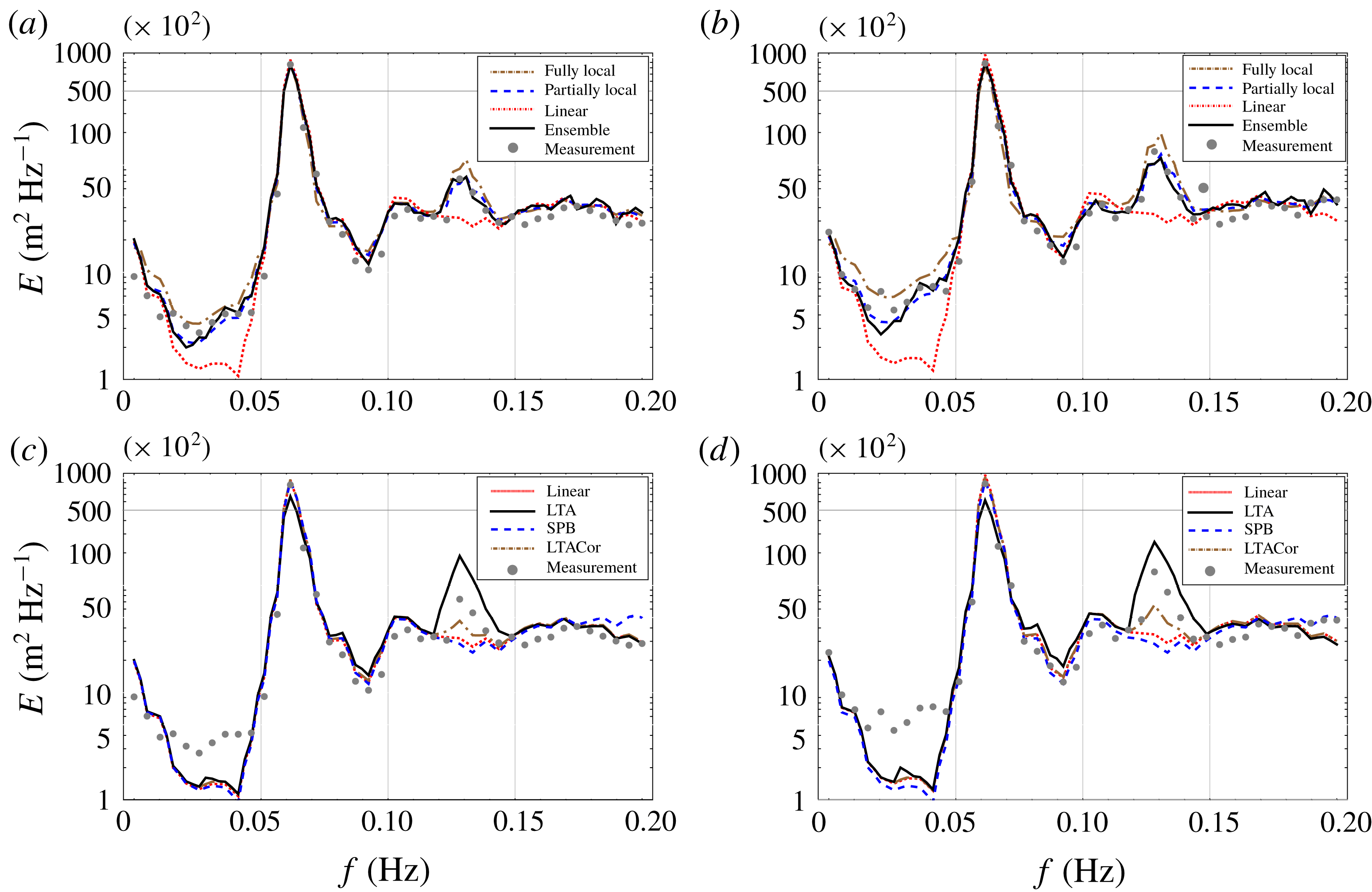
This case was simulated also in Vrecica & Toledo (Reference Vrecica and Toledo2016). The simulation is repeated in this work, but with finer discretization in frequency and space domains. By accounting for spectral changes in the bispectra, the accuracy of the model is significantly improved. The simulation is performed using the linear model, ensemble averaged deterministic model of Bredmose et al. (Reference Bredmose, Agnon, Madsen and Schaffer2005), fully local formulation using (3.24) and (3.25), and solution for the specific bathymetry using (C 3) and (C 6), without accounting for the dissipation and nonlinear effects. Both of the new formulations give similar results, although the partially local formulation performs better overall. It is possible for both of the presented formulations to save values of interaction coefficients at grid points, meaning that the computational costs of running the model are identical. Pre-calculation of the coefficients is more computationally intensive for the partially local formulation though. Results of the linear model are shown in order to demonstrate the magnitude of the nonlinear effects. The performance of LTA and SPB models is also tested, with and without corrections to the tuning parameter
 $\unicode[STIX]{x1D6FC}$
discussed in Salmon et al. (Reference Salmon, Smit, Janssen and Holthuijsen2016). A formulation which best fitted the measurements was used in each case.
The evolution of the spectrum for the models derived in this and a previous paper (see Vrecica & Toledo Reference Vrecica and Toledo2016), is shown in figure 1. The agreement between the numerical results and the measurements is very good, accounting for the generation of secondary and tertiary peaks, as well as the generation of the infragravity wave field. The fully local model grasps the essential properties of the wave field evolution, but is not as accurate as the partially local one. The SPB model is unable to account for transfer of energy to higher and infragravity frequencies. The original formulation of the LTA model overestimates the energy transfer by a large margin, while the corrected version under-predicts it. Both of these do not account for the generation of the infragravity wave field and the third peak.
Evolution of the unidirectional spectra over a sloping beach. The initial peak is at 0.06 Hz, and the wave variance
 $(\sum 1/2F^{2})$
is around
 $0.05~\text{m}^{2}$
. The spectrum is discretized in 80 bins. The grey dots represents the measurements of Freilich & Guza (Reference Freilich and Guza1984). In panels (a) and (b), the dotted red line represents the linear model, the black solid line is the ensemble averaged deterministic model, the dot-dashed brown line represents the fully local model based on (3.24) and (3.25) and the blue dashed line represents the partially local model based on (C 3) and (C 6). In panels (c) and (d) the dotted red line represents the linear model, the black solid line is the LTA model, the dot-dashed brown line is the LTA model with the correction of Salmon et al. (Reference Salmon, Smit, Janssen and Holthuijsen2016), and the blue dashed line represents the SPB model. The results are shown for depths of 5.25 m (a and c) and 4.1 m (b and d).

One thing to keep in mind is that the original formulation of the SPB model is not physical for certain conditions. This is due to a coefficient used by the model obtained in wave tank experiments
 $K=0.95k_{peak}-0.75$
, where
 $k_{peak}$
is peak wavenumber in deep water. It is possible to have a reversed transfer of energy for
 $k_{peak}>0.75/0.95$
, as in the following example. This issue is mitigated in most cases by using a formulation of the SPB model presented in Salmon et al. (Reference Salmon, Smit, Janssen and Holthuijsen2016), which uses local value of peak wavenumber.
4.2 Breaking of a unidirectional TMA spectrum over a slope
In this section shoaling and breaking of a unidirectional Texel, MARSEL, ARSLOE (TMA) (see Bouws et al. Reference Bouws, Günther, Rosenthal and Vincent1985) spectraum (case 4, table 1) over monotone slope is numerically investigated. The simulations correspond to the experimental case 28 from Smith (Reference Smith2004). The bathymetry is defined as
 $$\begin{eqnarray}\displaystyle h(x)=\{\begin{array}{@{}cc@{}}0.61-x/30 & 0<x\end{array}\}, & & \displaystyle\end{eqnarray}$$
with values expressed in metres. The initial significant wave height is 0.09 m, amplification factor is 100, and the peak period is 1.75 s. The input spectra and results of the measurements are obtained by digitization of the graphs from the original work.
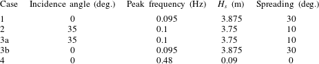
Cases under consideration for evolution of the 2-D spectra over a monotone slope. The column labelled ‘Case’ defines the number of the simulation. The spectrum for case 3 is defined as the sum of the two spectra 3a and 3b evolving together with their mutual nonlinear interactions. Incidence angle defines angle of peak wave direction to the onshore direction. Peak frequency represents
 $T_{p}$
.
 $H_{s}$
is the significant wave height. The column labelled ‘Spreading’ describes how much waves propagate around the mean direction; spreading of
 $30^{\circ }$
means they are propagating
 $\pm 15^{\circ }$
around
 $D_{p}$
following
 $\cos ^{2}$
distribution.

One of the forms of the dissipation term, fitting for the case under consideration is defined as
 $$\begin{eqnarray}\displaystyle & \displaystyle {\displaystyle \frac{\unicode[STIX]{x2202}a_{p}}{\unicode[STIX]{x2202}x}}=D_{p}a_{p},\quad D_{p}=c_{1}{\displaystyle \frac{D_{br}}{\sum C_{g,p}a_{p}/2}}a_{p}+c_{2}{\displaystyle \frac{D_{br}}{\sum C_{g,p}a_{p}/2}}{\displaystyle \frac{f_{p}^{2}}{f_{m02}}}a_{p}, & \displaystyle\end{eqnarray}$$
 $$\begin{eqnarray}\displaystyle D_{br}={\displaystyle \frac{1}{4}}f_{m01}(0.8h)^{2}Q,\quad {\displaystyle \frac{1-Q}{\ln (Q)}}=-{\displaystyle \frac{1}{2}}\left({\displaystyle \frac{H_{s}}{0.8h}}\right)^{2}, & & \displaystyle\end{eqnarray}$$
where
 $f_{m}$
is the mean weighted frequency,
 $f_{m2}$
is the mean square weighted frequency,
 $c_{1}$
and
 $c_{2}$
are tunable coefficients and
 $H_{s}$
is the significant wave height. First a total loss of energy
 $(D_{br})$
is calculated based on the formulation of Battjes & Janssen (Reference Battjes and Janssen1978). The most common approach is to equally distribute loss of energy across all spectral components, such as in Eldeberky & Battjes (Reference Eldeberky and Battjes1996) where
 $c_{1}=1$
and
 $c_{2}=0$
. However, the model shows better agreement with the frequency dependent formulation of Mase & Kirby (Reference Mase and Kirby1992) where
 $c_{1}=0.5$
and
 $c_{2}=0.5$
. It should be taken into account that the energy dissipation term
 $D_{p}$
is based on heuristics, therefore some tuning is necessary when changing the base model.
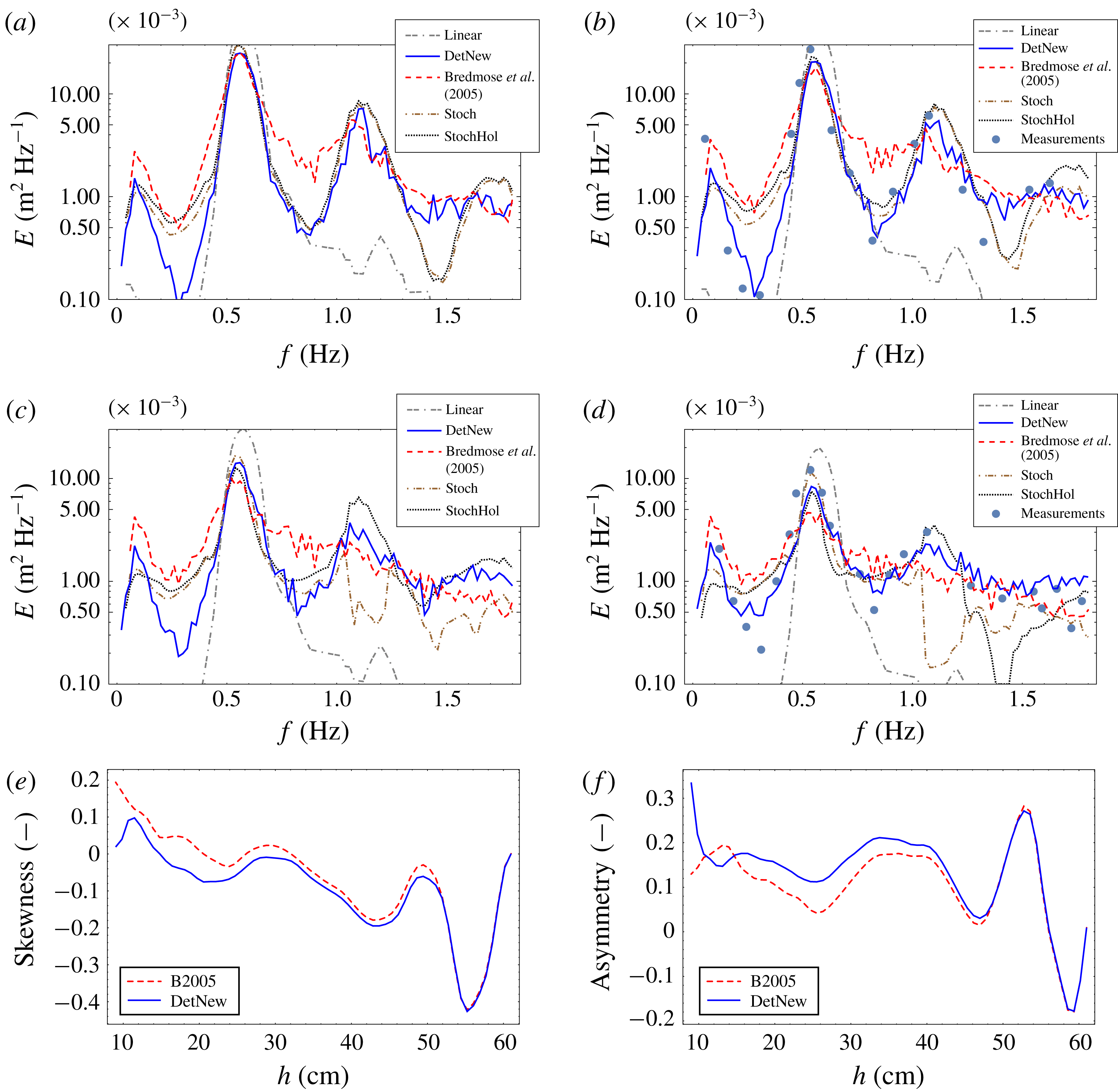
Initially, a secondary peak forms at double the frequency of the initial peak. As the water gets shallower, the waves start to break, leading to a significant loss of energy. The formation of a third peak at triple the frequency of the initial peak is not as clearly pronounced. A very clear peak forms in the infragravity range, with magnitude comparable to that of the secondary peak. Evolution of the initial spectra is modelled using an ensemble average obtained using the deterministic model of Bredmose et al. (Reference Bredmose, Agnon, Madsen and Schaffer2005), an ensemble average of the deterministic model presented in § 3.1, and for the results obtained using partially local formulation of the stochastic model, with the corrections presented in § 3.1.
As the closure of Benney & Saffman (Reference Benney and Saffman1966) over-predicts energy transfer, a stochastic simulation is also performed using a closure of Holloway (Reference Holloway1980). The closure is based on the empirical observations, and adds additional dissipation to the bispectrum evolution equation. Similar formulation to the one presented in Janssen (Reference Janssen2006) § 4.4 is used, however, only additional linear dissipation was added to the bispectrum evolution equation. This is straightforward to implement, only the dissipation coefficients in the bispectrum evolution equation (2.4) are modified (see appendix C). In total there are three different dissipation effects that are considered. The same as in Janssen, Herbers & Battjes (Reference Janssen, Herbers and Battjes2006), we include a dissipation term (
 $D$
) in the deterministic model, and additionally (
 $D2$
) in the bispectrum evolution equation (to model the effects of decorrelation). The difference is that we also consider the effect of dissipation in the nonlinear interaction term (
 $W$
) through implementation as an imaginary part of the wave number (see § 3.1).
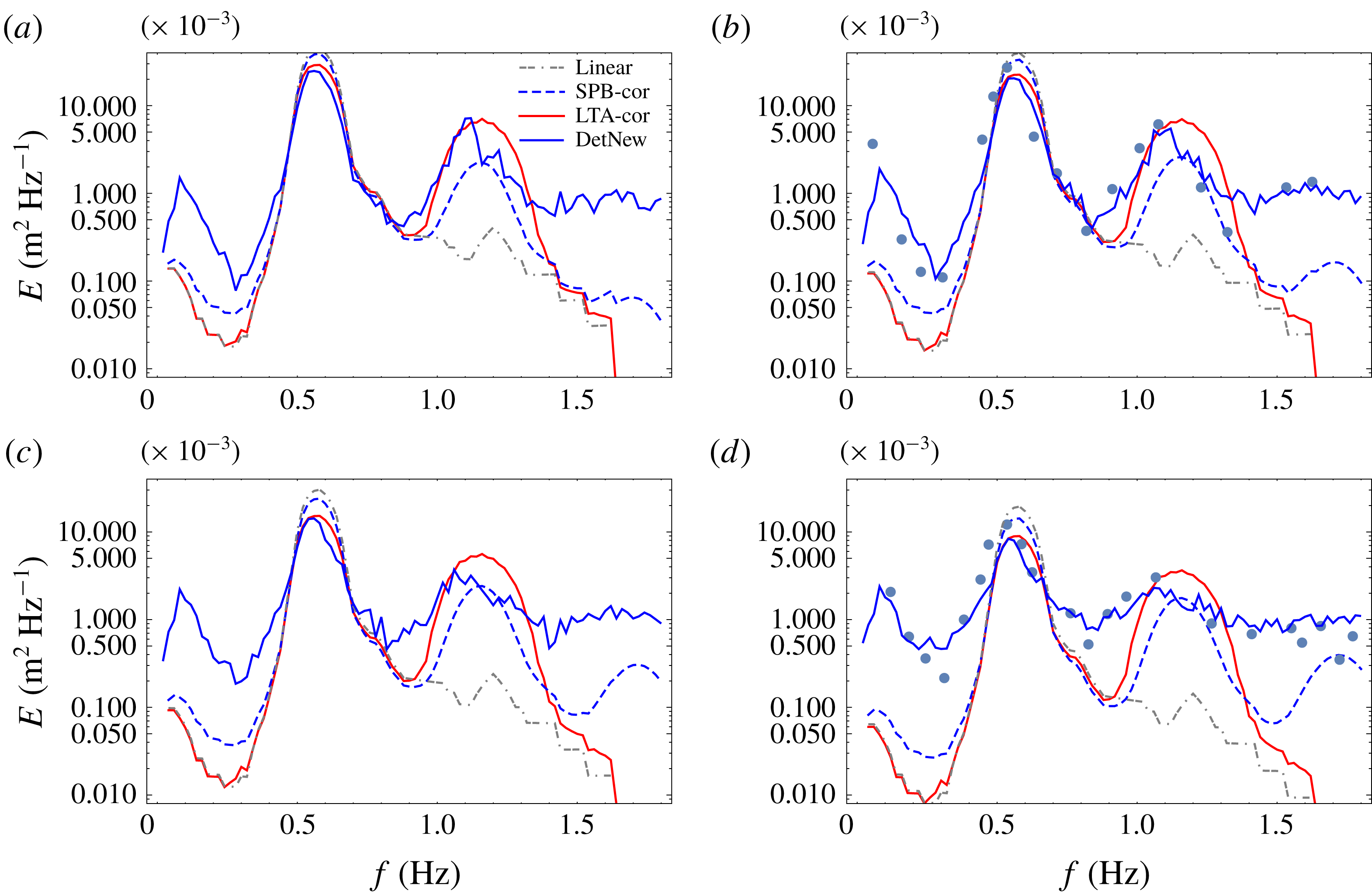
Results are shown in figure 2. In figure 3 results obtained using LTA and corrected SPB formulation are shown. Evolution of wave skewness and asymmetry, for an ensemble average of deterministic model, is shown in figure 2. It should be pointed out that although the agreement of the new models with the measurements is good, further work is needed in understanding wave dissipation and statistics in the nearshore.
Evolution of the unidirectional TMA spectra over the monotone slope, corresponding to the experimental case 28 from Smith (Reference Smith2004) (grey dots). The primary peak is at 0.58 Hz and the initial significant wave height is 9 cm. The ensemble average of deterministic model from § 3.1 is plotted as a solid blue line for the newly derived model, and dashed red colour for the ensemble average of Bredmose et al. (Reference Bredmose, Agnon, Madsen and Schaffer2005); the dash-dash-dot grey line is the linear model, the dot-dash-dot brown line is the stochastic model and the dotted black line is the output of the stochastic model with the closure of Holloway. The spectrum at water depths of 18 cm (a), 15 cm (b), 12 cm (c) and 9 cm (d) is shown. Evolution of ensemble averaged wave skewness (e) and asymmetry (f) is also shown, for both versions of the deterministic model.

Comparison between existing stochastic models for the same case shown in figure 2. In each panel a solid red line represents the LTA model, a dash-dot-dash grey line is the linear model, a solid blue line is the new formulation of deterministic model and a dashed blue line is the corrected SPB model. The grey dots represent the measurements. The spectrum at water depths of 18 cm (a), 15 cm (b), 12 cm (c), and 9 cm (d) is shown.

The ensemble average of the deterministic mild slope equation derived in § 3.1 shows much better agreement with the measurements in all frequency ranges of the spectra. The original formulation of Bredmose et al. (Reference Bredmose, Agnon, Madsen and Schaffer2005) significantly over-predicts the energy transfers. The stochastic models of the authors grasp the overall evolution of the wave field up to the 15 cm depth. However, as the water gets shallower the output of the stochastic model deviates significantly from measurements. The statistical properties of the deterministic model’s ensemble average shows that the closure of Benney & Saffman (Reference Benney and Saffman1966) fails in the breaking zone. A closure of Holloway (Reference Holloway1980) is applied to the model, as discussed in Janssen (Reference Janssen2006) § 4.4. The closure improved the prediction of the stochastic model, with regard to the primary and secondary peak generation. An initial examination shows that the error made by the closure of Benney & Saffman (Reference Benney and Saffman1966) is more evenly distributed, this is, however, beyond the scope of this work.
The LTA model and the corrected SPB model account for the generation of the secondary peak, but they fail to predict the generation of the infragravity wave peak. They also predict a very narrow spectral shape, as opposed to the measurements. The present CDB model is capable of grasping both.
Evolution of ensemble averaged wave skewness and asymmetry is shown in figure 2(e,f). Both skewness and asymmetry oscillate in deeper water, however, as the water gets shallower the two models diverge. For the model accounting for the slopes of the amplitudes, the skewness tends to asymptotically go to zero, while the asymmetry continues to increase, which is in line with field observations (see Elgar & Guza Reference Elgar and Guza1985). This is not the case with the other formulation of the deterministic model, in which the opposite happens.
4.3 Evolution of directionally spread JONSWAP spectra over a monotonous slope
The previous case shows good agreement of the model with measurements for 1-D approximation. The aim of this subsection is to verify qualitative behaviour of the model, and to investigate essential properties of 2-D wave shoaling. With this aim, four different cases are simulated, and all of them are presented in table 1. For all cases the spectrum is defined using the original formulation of the Joint North Sea Wave Observation Project (JONSWAP) spectra from Hasselmann, Dunckel & Ewing (Reference Hasselmann, Dunckel and Ewing1973) with
 $\cos ^{2}$
directional distribution, and an amplification factor of 3.3.
The bathymetry is defined as
 $$\begin{eqnarray}\displaystyle h(x)=\left\{\begin{array}{@{}cc@{}}50-0.05x & 0<x<900\\ 5 & x>900\end{array}\right\}, & & \displaystyle\end{eqnarray}$$
with values expressed in metres. As the goal of this subsection is to gain a better understanding of directional properties of the wave field, a simple local stochastic model (3.24) and (3.25) is used in the simulations.
It is important to note that discretization needs to be done carefully, especially in 2-D models. In order to account for resonant and near resonant interactions, the discretization needs to be fine enough (see Lvov, Nazarenko & Pokorni Reference Lvov, Nazarenko and Pokorni2006), which is fulfilled in this work. An issue that arises as waves enter shallow water is that no discretization is fine enough to account for resonant interactions. However, it was shown in Annenkov & Shrira (Reference Annenkov and Shrira2006) that accounting for near resonant interactions is of even higher importance.
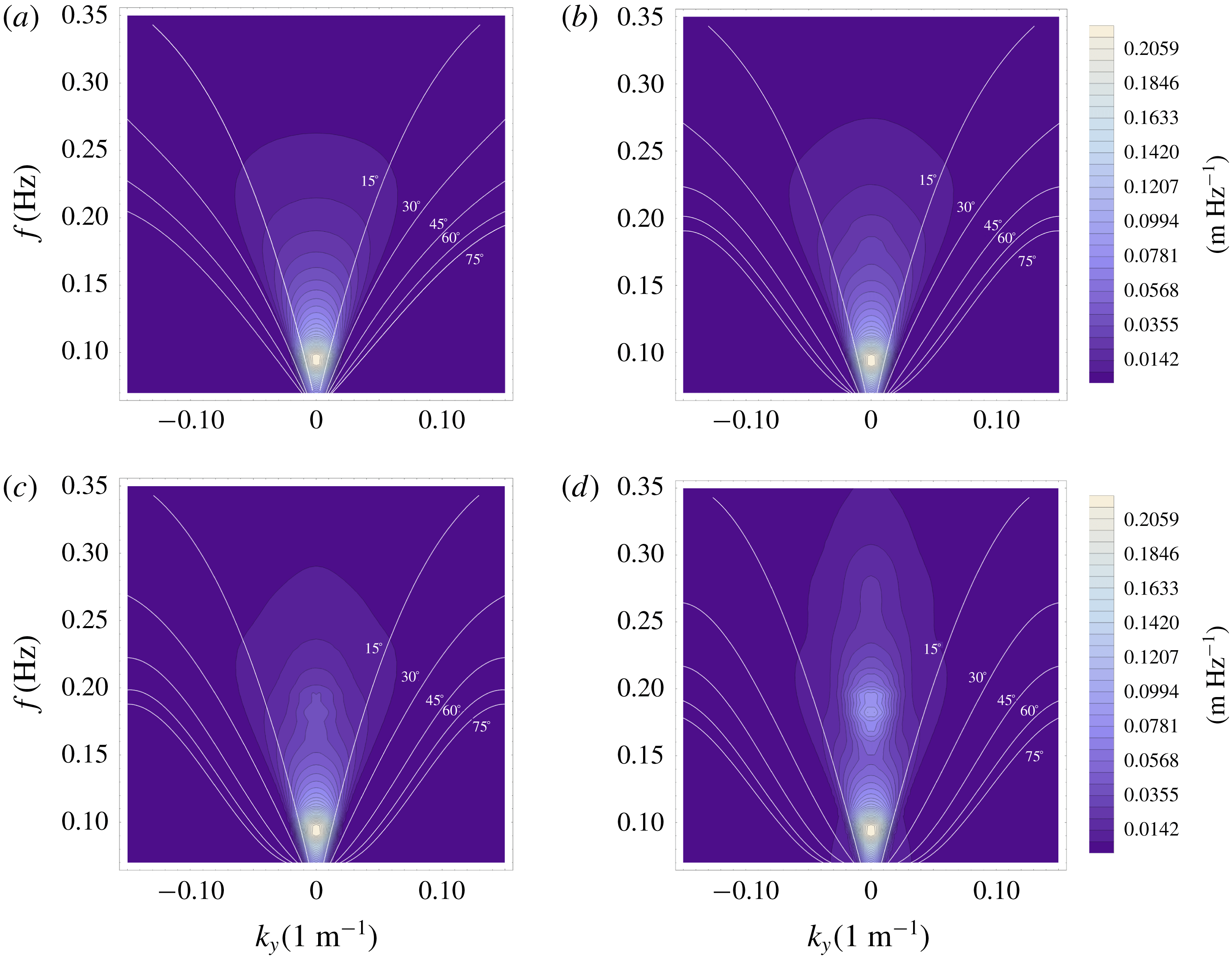
In case 1, a single 2-D JONSWAP spectrum with spreading of
 $\pm 15^{\circ }$
propagates over a monotone slope. The initial significant wave height is
 $H_{s}=3.85~\text{m}$
. The evolution of the single system propagating towards shore is shown in figure 4. As expected a secondary peak forms at double the frequency of the initial peak. A small peak at triple the frequency forms near the end of the propagation. It can be seen that the 2-D nonlinear spectral broadening of the peak discussed in Toledo (Reference Toledo2013), can be accounted for using the derived 2-D stochastic model. Similar results are given by Ma et al. (Reference Ma, Chen, Ma and Dong2017) using a Boussinesq model.
Amplitude spectrum of shoaling 2-D wave field. The system propagates onshore, has a peak at 0.095 Hz and directional spreading of
 $\pm 15^{\circ }$
. The initial significant height is 3.85 m.
 $k_{y}$
is the lateral wavenumber. White lines represent constant angle of incidence to the shoreline. The results are shown for water depths of 50 m (a), 20 m (b), 14 m (c) and 8 m (d).

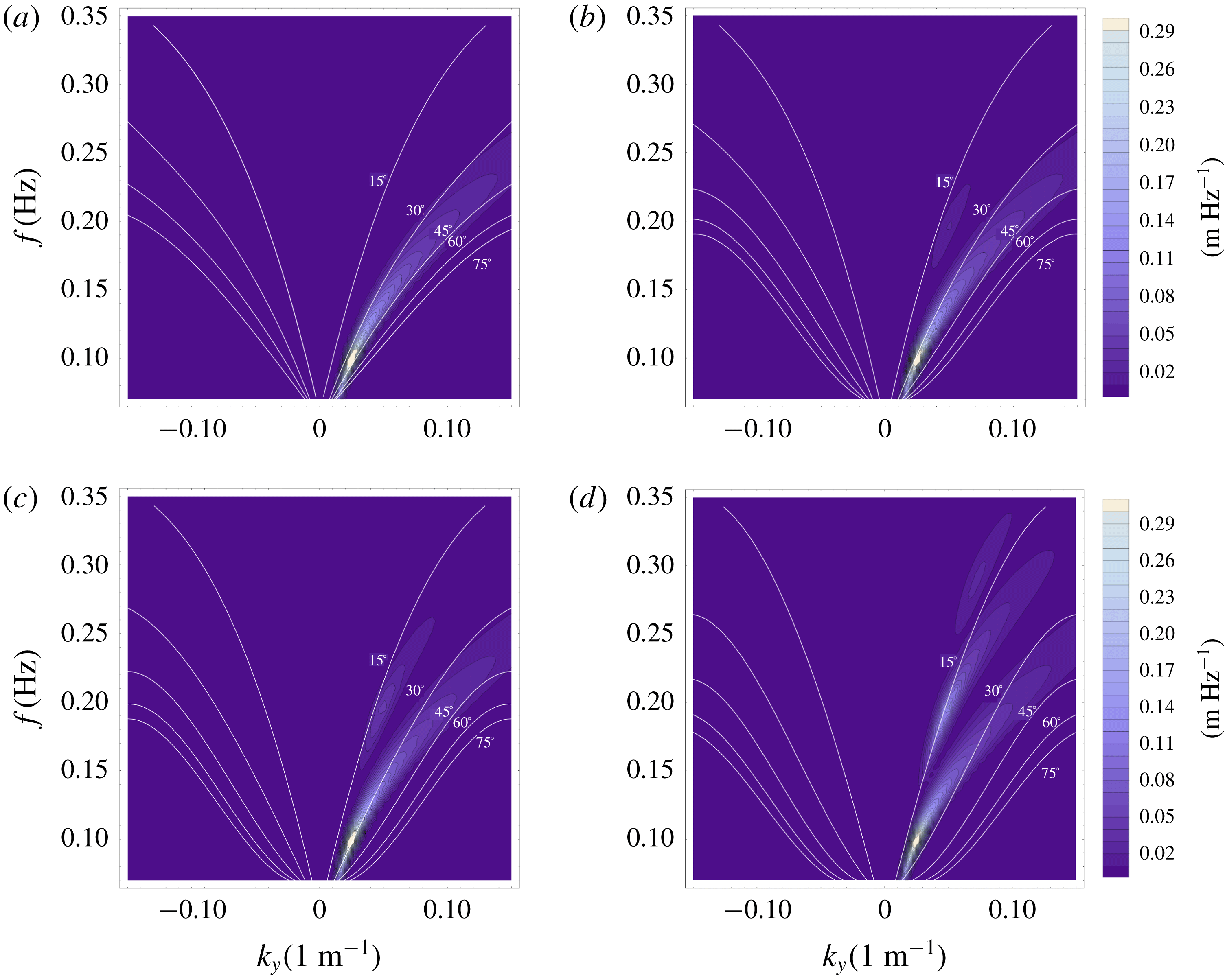
In case 2, a single 2-D JONSWAP spectrum with an initial angle of attack of
 $35^{\circ }$
and spreading of
 $\pm 10^{\circ }$
propagates over a monotone slope. The initial significant wave height is
 $H_{s}=3.75~\text{m}$
. The results are shown in figure 5. It should be noted that the intensity of the nonlinear interactions is reduced by a small amount for the system propagating at an angle to the onshore direction. This can be explained by the smaller effective bottom slope, and by the inability to close the direct resonance conditions as in the 1-D case.
Amplitude spectrum of shoaling 2-D wave field. The system propagates at
 $35^{\circ }$
angle to the shore, has a peak at 0.1 Hz and directional spreading of
 $\pm 10^{\circ }$
. The initial significant height is 3.75 m.
 $k_{y}$
is the lateral wavenumber. White lines represent constant angles of incidence to the shoreline. The results are shown for water depths of 50 m (a), 20 m (b), 14 m (c) and 8 m (d).

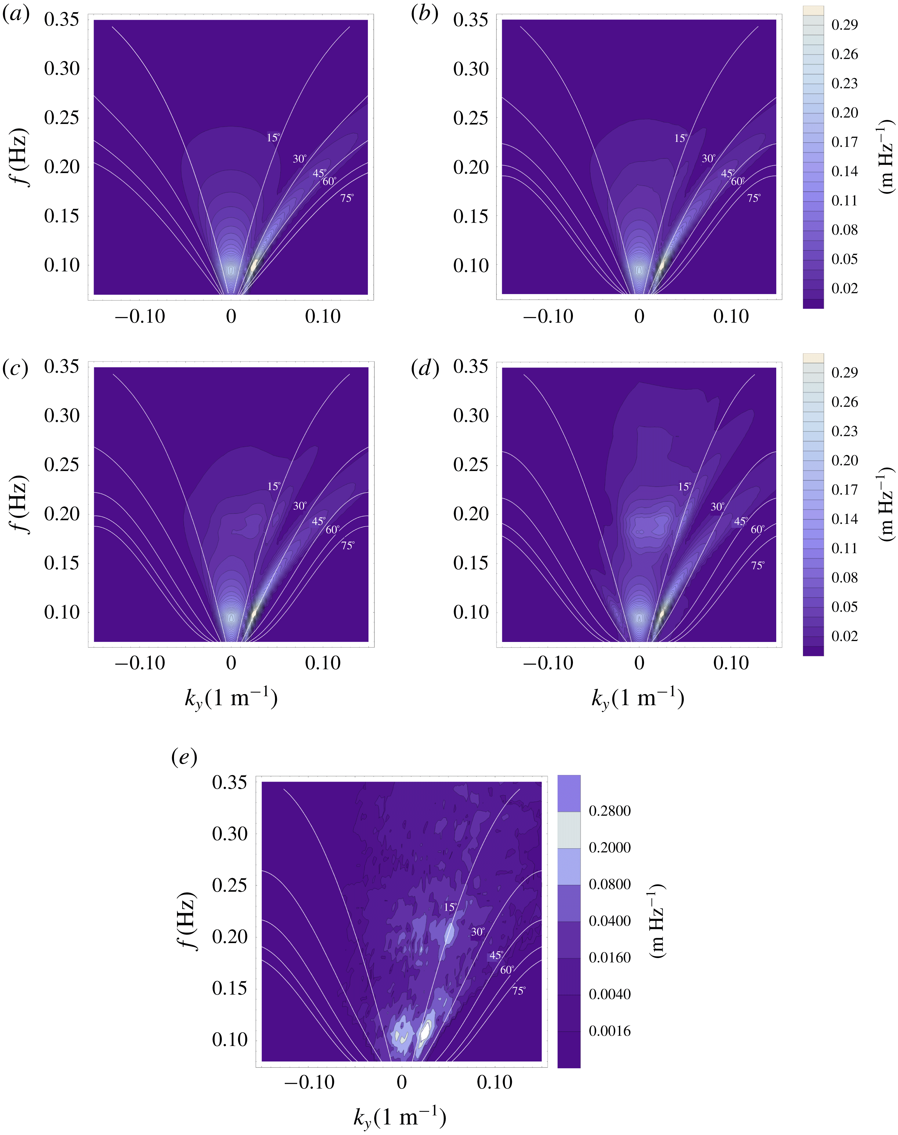
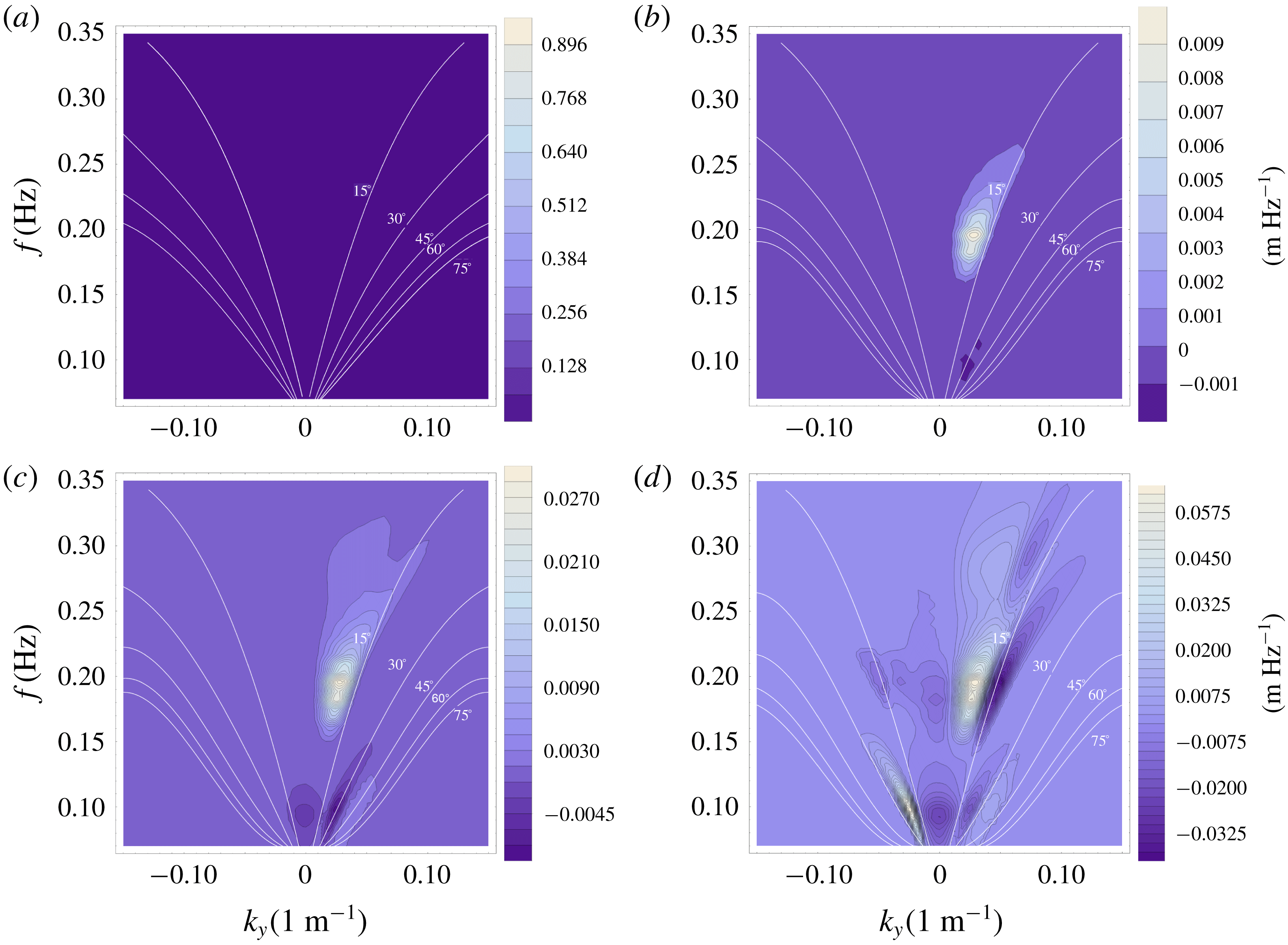
In case 3, a combination of the two previous JONSWAP spectra propagate over the same monotone slope. The two systems interact with themselves and with each other to generate three new secondary peaks with different intensities and directionalities. The spectrum also significantly broadens due to the subharmonic interactions. In order to show the effects of the interaction between the two systems, the difference between the two systems’ combined evolution and a sum of the two systems evolving independently is shown in figures 6 and 7.
Amplitude spectrum of shoaling 2-D wave field, and a realization of the deterministic model. This figure shows the evolution of the spectrum for the case of directionally spread seas. The initial spectrum is the sum of initial spectra from figures 4 and 5. White lines represent constant angle of incidence to the shoreline. The results are shown for water depths of 50 m (a), 20 m (b), 14 m (c) and 8 m (d). A realization of a deterministic model for a two system case at depth of 8 m is also shown (e).

Difference of the amplitude spectrum for the evolution of the whole system and sum of evolutions of two independent systems. The first system propagates at
 $35^{\circ }$
angle to the shore, has a peak at 0.1 Hz and directional spreading of
 $\pm 10^{\circ }$
. The second system propagates onshore, has a peak at 0.095 Hz and directional spreading of
 $\pm 30^{\circ }$
. The initial significant heights are 3.85 m and 3.75 m, respectively. White lines represent constant angles of incidence to the shoreline. The results are shown for water depths of 50 m (a), 20 m (b), 14 m (c) and 8 m (d).

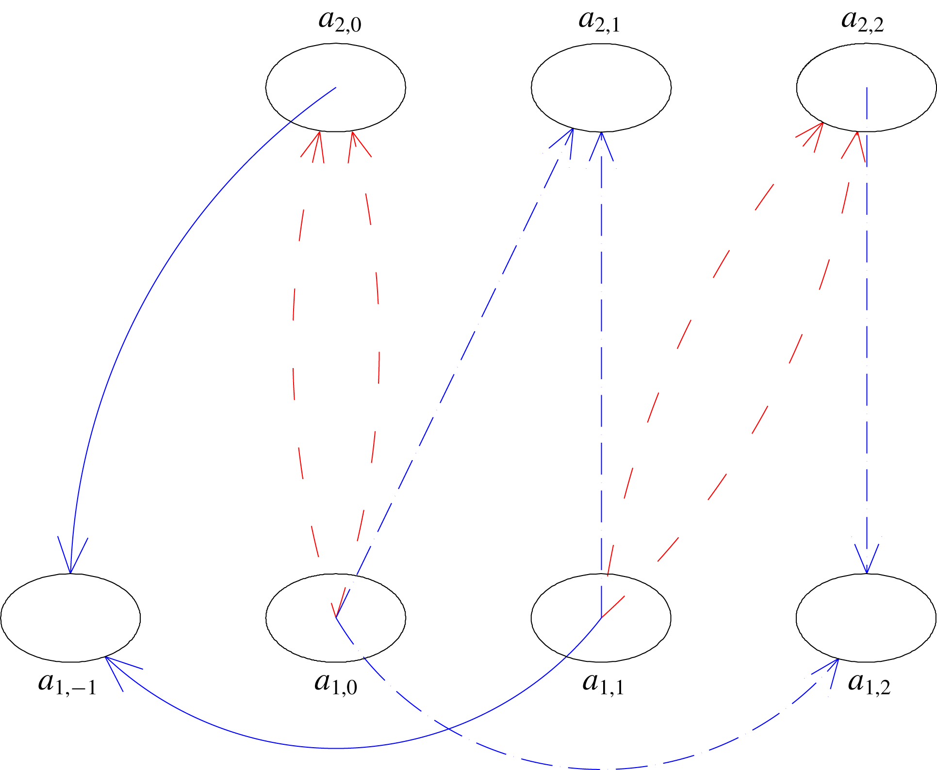
Wave triad interaction schematic in frequency–wavenumber space showing broadening of the spectrum for directionally spread seas. Generation of wave components in the opposite direction is shown using a solid blue line. Interactions between the two systems are shown using a dot-dashed blue line. Interactions of the system with itself are shown using a dashed red line.

Interesting directional properties of the wave field can be deduced from these figures. The directionality of the secondary peaks depends on the sum of the lateral wavenumbers of the primary peaks. More importantly, as a result of the subharmonic interactions between the primary peaks with the secondary peaks, the spectrum significantly broadens. Although this broadening is second-order in energy, it is first-order in direction. A similar behaviour, whose cause was not explained, can be found in the field measurements of Herbers et al. (Reference Herbers, Orzech, Elgar and Guza2003). A known cause of nonlinear spectrum broadening is the scattering due to bottom ripples (see Fabrice & Herbers Reference Fabrice and Herbers2002). Here, it is shown that also a uniform slope can cause nonlinear broadening. This property can also be qualitatively observed in an output of a single deterministic run corresponding to case 3 (see figure 6 e).
New wave components are generated at the frequency of the primary peaks, which have large attack angles compared to the original ones. Perhaps the most interesting effect is the generation of a peak with the mirrored angle of propagation. This is the result of a subharmonic interaction of a primary peak propagating at an angle and a secondary peak propagating directly to the shoreline. A schematic description of this mechanism is given in figure 8. Wave component
 $a_{1,0}$
generates its superharmonic
 $a_{2,0}$
through self-interaction. This allows the
 $a_{2,0}$
component and
 $a_{1,1}$
component to generate through subharmonic interaction
 $a_{1,-1}$
, which has an opposite angle of propagation compared to harmonic
 $a_{1,1}$
. This effect is shown using a solid blue line. Other interactions which only happen as a result of interactions between two wave systems are shown using dashed blue line. Interactions which do not depend on the existence of the other system are shown using a dashed red line. As discussed in Salmon et al. (Reference Salmon, Smit, Janssen and Holthuijsen2016), one of the biggest limitations of SPB and LTA is that they only account for interactions of co-propagating waves. This shows the importance of the capability of the current model for accounting for nonlinear wave interactions of waves propagating in all onshore directions.
5 Conclusions
The main achievements of this work are derivation of the localized 2-D nonlinear triad interaction source terms fitting for operational wave models (e.g. SWAN, WAVEWATCH), and improvement to the formulations of deterministic and non-local stochastic models.
Some of the observed qualitative wave evolution properties, previously unaccounted for by the operational models are described here. The most interesting 2-D property found in the numerical investigation is the generation of new harmonics through the process of subharmonic interaction. Propagation angles for these waves can be much larger than that of the wind sea, and for directionally spread seas it is possible to generate a new spectral peak, which has the opposite lateral direction of propagation compared to the incident oblique system. It was shown in Groeneweg et al. (Reference Groeneweg, van Gent, van Nieuwkoop and Toledo2015) that the new harmonics generated through these interactions can penetrate into areas thought to be protected and cause complications. Therefore it is important to know not only the total energy of the wave field and associated wave periods, but also its directionality.
New deterministic and stochastic formulations of the model are presented in this work. Most notably, by accounting for first-order changes of bathymetry and dissipation effects in the nonlinear term, the models viability is extended into the surf zone. The effect of spectrum changes in the stochastic model can be taken into account by using either a first- or second-order solution for the spectral components.
The work describes how to implement a model as a 2-D triad interaction source term (CDB model) in phase averaged large-scale wave forecasting models, such as SWAN, WAVEWATCH III, TOMAWAC, and WAM. Unlike the existing formulations, the CDB model is able to account for interactions of waves propagating in different directions, not just interactions of co-propagating waves. Further investigation of quantitative properties will be possible after implementation. The model’s biggest advantages lie in its localized nature and its consistency from deep water (in the vicinity of the nearshore region) to the breaking zone. It is able to describe three very different regimes, one in deep and intermediate waters where waves are mostly non-resonant, a transition regime where waves approach resonance between intermediate and shallow water, and propagation in relatively shallow waters.
Acknowledgements
This research was supported by the Israel Science Foundation (grant no. 1940/14) and Israel’s Ministry of Science and Technology (grant no. 3-12473).
Appendix A. Definitions of coefficients from Vrecica & Toledo (Reference Vrecica and Toledo2016)
Terms derived in Bredmose et al. (Reference Bredmose, Agnon, Madsen and Schaffer2005) and Vrecica & Toledo (Reference Vrecica and Toledo2016) are presented here. The details of the derivation can be found in previously mentioned works. The nonlinear interaction term
 $W$
, and its coefficients are
 $$\begin{eqnarray}\displaystyle & \displaystyle W_{s,p-s}=-{\displaystyle \frac{\unicode[STIX]{x1D714}_{p}}{g}}(k_{s,u}^{x}+k_{p-s,l-u}^{x}-k_{p,l}^{x})T_{s,p-s}^{(2)}+g{\displaystyle \frac{\unicode[STIX]{x1D714}_{p}}{\unicode[STIX]{x1D714}_{s}\unicode[STIX]{x1D714}_{p-s}}}H_{s,p-s}Y_{s,p-s}^{(2)}, & \displaystyle\end{eqnarray}$$
 $$\begin{eqnarray}\displaystyle & \displaystyle T_{s,p-s}^{(2)}={\displaystyle \frac{g^{2}k_{s}k_{p-s}}{2\unicode[STIX]{x1D714}_{p}\unicode[STIX]{x1D714}_{s}\unicode[STIX]{x1D714}_{p-s}}}-{\displaystyle \frac{1}{2}}\unicode[STIX]{x1D714}_{p}+{\displaystyle \frac{\unicode[STIX]{x1D714}_{s}\unicode[STIX]{x1D714}_{p-s}}{2\unicode[STIX]{x1D714}_{p}}}, & \displaystyle\end{eqnarray}$$
 $$\begin{eqnarray}\displaystyle & \displaystyle H_{s,p-s}={\displaystyle \frac{\text{i}k_{p,l}^{x}-\text{i}k_{s,u}-\text{i}k_{p-s,l-u}+D_{p,l}}{-\text{i}(k_{s,u}+k_{p-s,l-u})\tan (-\text{i}(k_{s,u}+k_{p-s,l-u})h)+k_{p,l}\tanh (hk_{p,l})}}, & \displaystyle\end{eqnarray}$$
 $$\begin{eqnarray}\displaystyle Y_{s,p-s,u,l-u}^{(2)} & = & \displaystyle {\displaystyle \frac{\text{i}}{2g^{3}}}\unicode[STIX]{x1D714}_{s}^{2}\unicode[STIX]{x1D714}_{p-s}^{2}\unicode[STIX]{x1D714}_{p}-{\displaystyle \frac{\text{i}}{2g^{3}}}\unicode[STIX]{x1D714}_{s}\unicode[STIX]{x1D714}_{p-s}\unicode[STIX]{x1D714}_{p}^{3}\nonumber\\ \displaystyle & & \displaystyle +\,{\displaystyle \frac{\text{i}}{g}}\unicode[STIX]{x1D714}_{p}(k_{s,u}^{x}k_{p-s,l-u}^{x}+k_{s,u}^{y}k_{p-s,l-u}^{y})+{\displaystyle \frac{\text{i}}{2g}}\unicode[STIX]{x1D714}_{p-s}k_{s,u}^{2}+{\displaystyle \frac{\text{i}}{2g}}\unicode[STIX]{x1D714}_{s}k_{p-s,l-u}^{2}.\end{eqnarray}$$
The linear shoaling term is defined as
 $$\begin{eqnarray}\displaystyle J_{s,u,p-s,l-u}=-{\displaystyle \frac{C_{g,p}^{\prime }}{2C_{g,p}}}-{\displaystyle \frac{C_{g,s}^{\prime }}{2C_{g,s}}}-{\displaystyle \frac{C_{g,p-s}^{\prime }}{2C_{g,p-s}}}. & & \displaystyle\end{eqnarray}$$
Appendix B. Definitions of new coefficients
The shallow water coupling coefficient is obtained in the same manner as in Vrecica & Toledo (Reference Vrecica and Toledo2016), but the definitions of
 ${\hat{W}}$
and
 $\tilde{J}$
terms are different. It is defined as
 $$\begin{eqnarray}\displaystyle \unicode[STIX]{x0394}Ps_{s,p-s,u,l-u}(x) & = & \displaystyle \text{Re}\left[{\displaystyle \frac{-W_{-s,-(p-s),u,l-u}}{\tilde{J}_{s,u,p-s,l-u}(x)}}\left(1-\sqrt{{\displaystyle \frac{C_{g,p}^{h_{g}}C_{g,s}C_{g,p-s}}{C_{g,p}C_{g,s}^{h_{g}}C_{g,p-s}^{h_{g}}}}}\right)\right.\nonumber\\ \displaystyle & & \displaystyle +\left(\sqrt{{\displaystyle \frac{C_{g,p}^{h_{g}}C_{g,s}C_{g,p-s}}{C_{g,p}C_{g,s}^{h_{g}}C_{g,p-s}^{h_{g}}}}}(1+{\hat{J}}_{s,u,p-s,l-u}^{h_{g}}(x))-1\right)\nonumber\\ \displaystyle & & \displaystyle \times \left({\displaystyle \frac{{\hat{W}}_{-s,-(p-s),u,l-u}}{\tilde{J}_{s,u,p-s,l-u}^{2}(x)}}-{\displaystyle \frac{W_{-s,-(p-s),u,l-u}\tilde{J}_{s,u,p-s,l-u}^{^{\prime }}(x)}{\tilde{J}_{s,u,p-s,l-u}^{3}(x)}}\right)\nonumber\\ \displaystyle & & \displaystyle +\left(-1+\sqrt{{\displaystyle \frac{C_{g,p}^{h_{g}}C_{g,s}C_{g,p-s}}{C_{g,p}C_{g,s}^{h_{g}}C_{g,p-s}^{h_{g}}}}}\left(1+{\hat{J}}_{s,u,p-s,l-u}^{h_{g}}(x)+{\displaystyle \frac{({\hat{J}}_{s,u,p-s,l-u}^{h_{g}}(x))^{2}}{2}}\right)\right)\nonumber\\ \displaystyle & & \displaystyle \times \left({\displaystyle \frac{-\hat{{\hat{W}}}_{-s,-(p-s),u,l-u}}{\tilde{J}_{s,u,p-s,l-u}^{3}(x)}}+{\displaystyle \frac{3{\hat{W}}_{-s,-(p-s),u,l-u}\tilde{J}_{s,u,p-s,l-u}^{^{\prime }}(x)}{\tilde{J}_{s,u,p-s,l-u}^{4}(x)}}\right.\nonumber\\ \displaystyle & & \displaystyle \left.\left.-\,{\displaystyle \frac{3{\hat{W}}_{-s,-(p-s),u,l-u}(\tilde{J}_{s,u,p-s,l-u}^{^{\prime }}(x))^{2}}{\tilde{J}_{s,u,p-s,l-u}^{5}(x)}}+{\displaystyle \frac{W_{-s,-(p-s),u,l-u}\tilde{J}_{s,u,p-s,l-u}^{^{\prime \prime }}(x)}{\tilde{J}_{s,u,p-s,l-u}^{4}(x)}}\right)\right].\nonumber\\ \displaystyle & & \displaystyle\end{eqnarray}$$
The
 ${\hat{W}}$
and
 $\hat{{\hat{W}}}$
terms which are defined as
 $$\begin{eqnarray}\displaystyle & \displaystyle {\hat{W}}_{s,p-s,u,l-u}=-{\displaystyle \frac{\unicode[STIX]{x2202}}{\unicode[STIX]{x2202}x}}(W_{s,p-s,u,l-u}\text{e}^{\text{i}\int \unicode[STIX]{x1D709}\,\text{d}x})/\text{e}^{\text{i}\int \unicode[STIX]{x1D709}\,\text{d}x}, & \displaystyle\end{eqnarray}$$
 $$\begin{eqnarray}\displaystyle & \displaystyle \hat{{\hat{W}}}_{s,p-s,u,l-u}=-{\displaystyle \frac{\unicode[STIX]{x2202}^{2}}{\unicode[STIX]{x2202}x^{2}}}(W_{s,p-s,u,l-u}\text{e}^{\text{i}\int \unicode[STIX]{x1D709}\,\text{d}x})/\text{e}^{\text{i}\int \unicode[STIX]{x1D709}\,\text{d}x}. & \displaystyle\end{eqnarray}$$
The
 $\tilde{J}$
term represents the sum of the linear shoaling terms in the bispectrum evolution equation and it is defined in this work as
 $$\begin{eqnarray}\displaystyle & \displaystyle \tilde{J}_{s,u,p-s,l-u}=-{\displaystyle \frac{C_{g,p}^{\prime }}{2C_{g,p}}}+{\displaystyle \frac{C_{g,s}^{\prime }}{2C_{g,s}}}+{\displaystyle \frac{C_{g,p-s}^{\prime }}{2C_{g,p-s}}}, & \displaystyle\end{eqnarray}$$
 $$\begin{eqnarray}\displaystyle & \displaystyle {\hat{J}}_{s,u,p-s,l-u}^{h_{g}}={\displaystyle \frac{1}{2}}\ln {\displaystyle \frac{C_{g,p-s}^{h_{g}}C_{g,s}^{h_{g}}C_{g,p}}{C_{g,p-s}C_{g,s}C_{g,p}^{h_{g}}}}. & \displaystyle\end{eqnarray}$$
The
 $\tilde{J}$
-term used in the shallow water expansion can go to zero at a certain point. A solution for this is to add an additional condition in the gate term, which is to set the minimum value of the
 $\tilde{J}$
-term to a small positive value
 $$\begin{eqnarray}\displaystyle \tilde{J}_{s,u,p-s,l-u}>\unicode[STIX]{x1D716}. & & \displaystyle\end{eqnarray}$$
 $h_{g}$
is defined as depth at which the shallow water localization activates. It is formulated as
 $$\begin{eqnarray}\displaystyle & & \displaystyle \text{Abs}\left(\text{Re}\left[{\displaystyle \frac{\text{d}^{2}}{\text{d}\unicode[STIX]{x1D709}^{2}}}{\displaystyle \frac{W_{-s,-(p-s),u,l-u}}{k_{s,u}^{x}+k_{p-s,l-u}^{x}-k_{p,l}^{x}+\text{i}\tilde{J}_{s,u,p-s,l-u}}}\right]\big/\right.\nonumber\\ \displaystyle & & \displaystyle \left.\text{Re}\left[{\displaystyle \frac{W_{-s,-(p-s),u,l-u}}{k_{s,u}^{x}+k_{p-s,l-u}^{x}-k_{p,l}^{x}+iJ_{s,u,p-s,l-u}}}\right]\right)>c,\end{eqnarray}$$
where
 $c$
is a constant, whose value is recommended as 0.5. An additional consideration for the gate term is that the
 $\tilde{J}$
-term cannot be zero, as this results in a singularity. In those cases it is recommended setting the value of the coupling term to zero.
The exponent of the wavenumber mismatch is approximated using Taylor series as
 $$\begin{eqnarray}\displaystyle \int _{h(x_{0})}^{h(x)}\unicode[STIX]{x1D709}(x^{\prime })\,\text{d}x^{\prime }=\unicode[STIX]{x1D709}(x){\displaystyle \frac{h(x_{0})-h(x)}{h^{\prime }(x)}}+{\displaystyle \frac{1}{2}}\unicode[STIX]{x1D709}^{^{\prime }}(x){\displaystyle \frac{(h(x_{0})-h(x))^{2}}{h^{\prime }(x)}}+\cdots & & \displaystyle\end{eqnarray}$$
Appendix C. Alternative formulations of the source term
In this appendix a way to account for nonlinear and dissipation effects in the coupling term is presented. A new numerical scheme which accounts for changes of bathymetry is derived. The presented approach is also more accurate for sharp changes in wave energy, such as for wave breaking cases.
C.1 Incorporation of nonlinear and dissipation effects
The first step in accounting for the nonlinear effects is to transform (3.18) into
 $$\begin{eqnarray}\displaystyle & \displaystyle E_{p,l}(x)=\text{e}^{\int _{0}^{x}D_{p}+NL_{p}\,\text{d}x^{\prime }}{\displaystyle \frac{C_{g,p}(0)}{C_{g,p}(x)}}E_{p,l}(0), & \displaystyle\end{eqnarray}$$
 $$\begin{eqnarray}\displaystyle & \displaystyle NL_{p}(x)={\displaystyle \frac{S_{nl,3,p}}{E_{p,l}(x)C_{g,p}(x)}}, & \displaystyle\end{eqnarray}$$
where
 $NL_{p}$
term represents the triad interactions, transformed into a form of a linear term. This is only applicable for non-zero
 $E_{p}$
components, for
 $E_{p}=0$
nonlinear effects are discarded. For the intermediate water localization, the effects of the linear shoaling dissipation and nonlinearity are simply incorporated into a
 $J$
-term as
 $$\begin{eqnarray}\displaystyle P_{s,p-s,u,l-u}(x) & = & \displaystyle \text{Re}\left[{\displaystyle \frac{-\text{i}W_{-s,-(p-s),u,l-u}}{\unicode[STIX]{x1D709}+\text{i}{\hat{J}}_{s,u,p-s,l-u}}}+{\displaystyle \frac{W_{-s,-(p-s),u,l-u}^{^{\prime }}}{(\unicode[STIX]{x1D709}+\text{i}{\hat{J}}_{s,u,p-s,l-u})^{2}}}\right.\nonumber\\ \displaystyle & & \displaystyle \left.-\,{\displaystyle \frac{W_{-s,-(p-s),u,l-u}}{(\unicode[STIX]{x1D709}+\text{i}{\hat{J}}_{s,u,p-s,l-u})^{3}}}{\displaystyle \frac{\text{d}(\unicode[STIX]{x1D709}+\text{i}{\hat{J}}_{s,u,p-s,l-u})}{\text{d}x}}\right]^{x}=\unicode[STIX]{x0394}\hat{P\text{i}}_{s,p-s,u,l-u}(x),\end{eqnarray}$$
 $$\begin{eqnarray}\displaystyle {\hat{J}}_{s,u,p-s,l-u} & = & \displaystyle \left(-{\displaystyle \frac{C_{g,p}^{\prime }}{2C_{g,p}}}+{\displaystyle \frac{C_{g,s}^{\prime }}{2C_{g,s}}}+{\displaystyle \frac{C_{g,p-s}^{\prime }}{2C_{g,p-s}}}\right)\nonumber\\ \displaystyle & & \displaystyle +\,(D_{p,l}-D_{s,u}-D_{p-s,l-u})+(-NL_{s,u}-NL_{p-s,l-u}).\end{eqnarray}$$
For the shallow water localization, these effects are incorporated into the
 $\unicode[STIX]{x1D709}$
term as
 $$\begin{eqnarray}\displaystyle P_{s,p-s,r,l-r}(x) & = & \displaystyle \sqrt{{\displaystyle \frac{C_{g,p}^{x_{0}}C_{g,s}C_{g,p-s}}{C_{g,p}C_{g,s}^{x_{0}}C_{g,p-s}^{x_{0}}}}}\nonumber\\ \displaystyle & & \displaystyle \times \,(\text{e}^{-\text{i}\int _{x_{g}}^{x}\hat{\unicode[STIX]{x1D709}}(x^{\prime })\,\text{d}x^{\prime }}P_{s,p-s,r,l-r}(x_{g})+\text{e}^{-\text{i}\int _{x_{g}}^{x}\hat{\unicode[STIX]{x1D709}}(x^{\prime })\,\text{d}x^{\prime }}\unicode[STIX]{x0394}\hat{Ps}_{s,p-s,u,l-u}^{x_{g},x}),\end{eqnarray}$$
 $$\begin{eqnarray}\displaystyle \hat{\unicode[STIX]{x1D709}}=\unicode[STIX]{x1D709}+(D_{p,l}-D_{s,u}-D_{p-s,l-u})+(-NL_{s,u}-NL_{p-s,l-u}). & & \displaystyle\end{eqnarray}$$
The formulation of the
 $\unicode[STIX]{x0394}\hat{Ps}$
-term is almost identical to the formulation of the
 $\unicode[STIX]{x0394}Ps$
-term, with the exception of replacing the
 $\unicode[STIX]{x1D709}$
-terms with the
 $\hat{\unicode[STIX]{x1D709}}$
-terms. Note that the exponents of the
 $\hat{\unicode[STIX]{x1D709}}$
-terms in equation (C 6) cancel each other, only the value of their derivatives remain in the localized
 $\unicode[STIX]{x0394}Ps$
-term.
Equations (C 3) and (C 6) allow the calculation of nonlinear coupling terms for sharply changing wave fields. Most breaking cases, and cases with high Ursell numbers fit this category. This version model requires transportation of nonlinear terms and dissipation, as their values cannot be calculated a priori. This, however, has a small numerical cost.
C.2 Formulation of the model accounting for sharp changes
In Vrecica & Toledo (Reference Vrecica and Toledo2016) the value of the interaction coefficient was determined solely based on the local slope and depth. This approach is appropriate for uniform or mildly varying slopes. In the case of sharp changes in the bathymetry, differences between non-local and local coefficients obtained in this manner can be large. Strong changes, due to the nonlinear or breaking effects, can also pose a problem. The formulation of the intermediate definition of the
 $\unicode[STIX]{x0394}P$
-term is identical to (3.24) and (C 3). The energy transfer is induced by bottom changes in the intermediate water, however, the waves are still far from resonance and do not build up correlations.
The new formulation
 $P$
-term in shallow water is, in a sense, similar to the non-local formulation. It transports the value of nonlinear coupling term (essentially a mean part of the bispectrum) along with the spectrum components. The shallow localization is used between the two points. In this way the Nyquist limitation is still overcome. The shallow water localized term is defined as
 $$\begin{eqnarray}\displaystyle P_{s,p-s,r,l-r}(x) & = & \displaystyle P_{s,p-s,r,l-r}(x_{0})\text{e}^{-\text{i}\int _{x_{0}}^{x}\unicode[STIX]{x1D709}(x^{\prime })\,\text{d}x^{\prime }}\nonumber\\ \displaystyle & & \displaystyle \times \,\sqrt{{\displaystyle \frac{C_{g,p}^{x_{0}}C_{g,s}C_{g,p-s}}{C_{g,p}C_{g,s}^{x_{0}}C_{g,p-s}^{x_{0}}}}}+\unicode[STIX]{x0394}Ps_{s,p-s,u,l-u}^{x_{0},x},\end{eqnarray}$$
where
 $P_{s,p-s,r,l-r}(x_{0})$
is the value of the coupling term at the previous spatial step (
 $x_{0}$
). It is possible to apply (3.25) (for milder sea conditions) or (C 6) (for cases with strong energy dissipation or nonlinearity) for the definition of the
 $\unicode[STIX]{x1D709}$
-term and the
 $\unicode[STIX]{x0394}Ps$
-term.
When a wave field enters the breaking zone, a spatial step needs to be small enough to account for breaking effects. In these cases it is recommended to run either a non-local stochastic model, or an ensemble average of the deterministic model. To get the most out of the localized approach in breaking cases, it is suggested using an unstructured grid for which the spatial step decreases as the wave field approaches the breaking zone, or to use larger grid spacing for the stochastic model and to interpolate the model output.
C.3 The closure of Holloway
In order to account for the overestimation of energy transfer, the closure of Holloway (Reference Holloway1980) is used in the same manner as in Janssen et al. (Reference Janssen, Herbers and Battjes2006). The application of closure entails adding additional dissipation to the bispectrum evolution equation (2.4). The equation itself remains the same, but an additional linear decorrelation term is used. It is defined here as
 $$\begin{eqnarray}\displaystyle D2_{p,s,p-s}={\displaystyle \frac{1}{2}}\left({\displaystyle \frac{D_{p}E_{p}+D_{s}E_{s}+D_{p-s}E_{p-s}+NL_{p}+NL_{s}+NL_{p-s}}{E_{p}+E_{s}+E_{p-s}}}\right), & & \displaystyle\end{eqnarray}$$
where
 $NL_{p}$
represents the absolute value of total nonlinear energy transfer to the wave component.
All other procedures remain the same, the additional term behaves identically to the linear dissipation terms (
 $D$
), and is summed up with them. It should be stressed that this closure is empirical, and different formulations could be used as well.
Appendix D. Implementation of the localized quasi-two-dimensional formulation as a full 2-D
 $S_{3nl}$
source term

The process of implementing the nonlinear triad interaction source term into operational wave forecasting models is discussed, and a short overview of the computational costs is given.
D.1 Bridging between the discretization scheme of the present model and the ones in forecasting models
The operational wave models describe the evolution of wave action in time and space. The area under consideration is represented as structured, unstructured or some other form of grid. The spectrum at each point of the grid is discretized in frequency (or wavenumber) and direction domains by using angle of propagation (WAVEWATCH, SWAN), or 2-D wavenumbers (TOMAWAC).
The first step in implementing the nonlinear source term is to define the direction of the biggest change in the bathymetry (
 $\unicode[STIX]{x1D6FE}$
) at each point. All of the interacting wave components are assumed to propagate at
 $\pm 90^{\circ }$
angle from the
 $\unicode[STIX]{x1D6FE}$
axis. As the wave field shoals, most of the wave energy travels in the general onshore direction due to the refraction, therefore this approach should be appropriate for most situations.
There are several differences that need to be bridged in order to use the present model as a triad source term (
 $S_{3nl}$
) in WAE models. The frequency spectrum used in operational models is sometimes discretized using a logarithmic scale, which differs from the linear scale used in the presented model. In TOMAWAC models the wave directionality is described in wavenumber space. However, in most other models the direction of each wave component is defined with the angle of propagation. In this model, the directionality is described by the magnitude of the lateral wavenumber with respect to
 $\unicode[STIX]{x1D6FE}$
. One of the possible approaches to resolve different discretization methods is to independently run the main wave action model and the triad source term.
Before the actual run, the coupling terms can be precalculated for the specified spectral and spatial grid (or their rate of change in case nonlinear and dissipation effects are accounted for). It is important to note that the coupling terms (
 $P$
) are also refracted in the same manner as the spectral components. The main model (see (D 1)) is then run, and it outputs the necessary information to the triad model. The value of the triad interaction source term is then calculated at every grid point, and outputted back to the main model, after multiplying it with
 $\text{cos}(\unicode[STIX]{x1D6FE})$
(see figure 9 for a schematic description).
Schematic detailing a possible implementation of the triad source term model into large-scale WAE models. The blue text and arrows indicate steps that are used both when
 $Q$
-terms are precalculated and when their change is partially precalculated between grid points. The white ones indicate steps that are needed for pre-computing the change of coefficients (when change due to nonlinearity and dissipation is tracked).

The main wave model, for the wave field without current, can be defined as
 $$\begin{eqnarray}\displaystyle {\displaystyle \frac{\unicode[STIX]{x2202}{\mathcal{A}}}{\unicode[STIX]{x2202}t}}+\unicode[STIX]{x1D735}\boldsymbol{\cdot }(\overrightarrow{C}_{g,p}{\mathcal{A}}_{p,l})+{\displaystyle \frac{\unicode[STIX]{x2202}}{\unicode[STIX]{x2202}k}}\dot{k}{\mathcal{A}}+{\displaystyle \frac{\unicode[STIX]{x2202}}{\unicode[STIX]{x2202}\unicode[STIX]{x1D703}}}\dot{\unicode[STIX]{x1D703}}{\mathcal{A}}=\sum S+\text{cos}(\unicode[STIX]{x1D6FE})S_{p,l}, & & \displaystyle\end{eqnarray}$$
where
 $\dot{k}$
represents shift of wave action to different wavelengths due to shoaling,
 $\dot{\unicode[STIX]{x1D703}}$
is the refraction term,
 $\text{cos}(\unicode[STIX]{x1D6FE})S_{p,l}$
is the triad source term and
 $\sum S$
represents other source terms. This formulation corresponds to that of WAVEWATCH III. The formulation of the source term in the
 $\unicode[STIX]{x1D6FE}$
direction is given for 1-D and 2-D formulations of the model. The 2-D formulation is defined as
 $$\begin{eqnarray}\displaystyle S_{p,l} & = & \displaystyle \mathop{\sum }_{s=p-N}^{N}\mathop{\sum }_{r=l-M}^{M}E_{s,r}E_{p-s,r-l}{\displaystyle \frac{\text{Re}[P_{s,p-s,r,l-r}W_{s,p-s,r,l-r}]C_{g,p}}{\unicode[STIX]{x1D714}_{p}}}\nonumber\\ \displaystyle & & \displaystyle +\,E_{s,r}E_{p,l}{\displaystyle \frac{\text{Re}[P_{p,p-s,l,l-r}W_{s,p-s,r,l-r}]C_{g,p}}{\unicode[STIX]{x1D714}_{p}}}\nonumber\\ \displaystyle & & \displaystyle +\,E_{p,l}E_{p-s,r-l}{\displaystyle \frac{\text{Re}[P_{s,p-s,r,l-r}W_{s,p-s,r,l-r}]C_{g,p}}{\unicode[STIX]{x1D714}_{p}}}.\end{eqnarray}$$
This formulation is fitting for most realistic cases, as wave fields commonly show strong 2-D properties (e.g. crossing seas). It should be noted that it is possible to evaluate coefficients using a quasi-two-dimensional assumption for mostly uniform beaches, while for more complicated cases, it is necessary to also refract the coupling terms together with the spectral components.
For simple test cases, or unidirectional wave spectra, the 1-D version of the model can be used. It is defined as
 $$\begin{eqnarray}\displaystyle S_{p} & = & \displaystyle \mathop{\sum }_{s=p-N}^{N}E_{s}E_{p-s}{\displaystyle \frac{\text{Re}[P_{s,p-s}W_{s,p-s}]C_{g,p}}{\unicode[STIX]{x1D714}_{p}}}\nonumber\\ \displaystyle & & \displaystyle +\,E_{s}E_{p}{\displaystyle \frac{\text{Re}[P_{p,p-s}W_{s,p-s}]C_{g,p}}{\unicode[STIX]{x1D714}_{p}}}+E_{p}E_{p-s}{\displaystyle \frac{\text{Re}[P_{s,p-s}W_{s,p-s}]C_{g,p}}{\unicode[STIX]{x1D714}_{p}}}.\end{eqnarray}$$
Equations (D 2) and (D 3) are the final main result of this work. While, as discussed above, there is still room for improvement (for example accounting for the effects of coherent wave patterns or currents), they are the basis for implementation of the triad source term into the operational wave model.
D.2 Computational costs
The main issue for the implementation of two-equation models comes from the associated computational cost. For example, in a 1-D case for a spectrum discretized in
 $N$
frequency bins, it is necessary to solve
 $N^{2}/6$
bispectrum evolution equations. In addition, this will require also a very dense spatial grid in order to resolve bi-spectral undulations. For operational wave models, which utilize hundreds of discretized wave components, it is unfitting for operational purposes to run two-equation models with the currently available computational resources. Localized one-equation models overcome this limitation by integrating the bispectrum evolution equation and extracting only the mean contribution of the resulting integral, so that the computational cost is significantly reduced.
In order to account for all possible forward interactions, it is necessary to use double summations, in frequency and direction (or wavenumber) domains. This is a significant computational cost; however, by utilizing the approach of Davis et al. (Reference Davis, Sheremet, Tian and Saxena2014), where the interacting triads are determined beforehand, it is possible to further reduce computational costs.
The localization procedure was first developed by Stiassnie & Drimer (Reference Stiassnie and Drimer2006) and improved in Toledo & Agnon (Reference Toledo and Agnon2012). However, while this approach works in the intermediate water, it fails once waves enter shallow water. In order to overcome this, a new procedure was developed for shallow water in Vrecica & Toledo (Reference Vrecica and Toledo2016) which asymptotically approximates the integral and connects it with the intermediate water area using the gate term.
The localized interaction coefficient depends only on the local values of the spectrum. The non-local versions requires history of dissipation and nonlinear source terms which need to be transported. It is possible to precompute the coupling terms (local) or their change over large distances (non-local) for a specific bathymetry and save the results to a database. For the operational runs, the coefficients can be retrieved from the database. This procedure lowers the cost of running the model by one order of magnitude, enough to potentially be used in operational wave modelling.