1 Introduction
The concept of ‘turbulent flashes’ in the region of transition from laminar to turbulent flow in pipes is one of the more puzzling outcomes of Reynolds’s (Reference Reynolds1883) seminal experiments using dye injected at the centreline of the inlet. He noted, ‘Another phenomenon … was the intermittent character of the disturbance. The disturbance would suddenly come on through a certain length of the tube and pass away and then come on again, giving the appearance of flashes.’ The disturbances would first appear as wavering regions of the dye filament, followed by the formation of successive, concentrated patches of dye downstream. In a series of experimental studies using optical methods, Lindgren (Reference Lindgren1953, Reference Lindgren1959a,Reference Lindgrenb,Reference Lindgrenc) systematically improved and extended the observations of Reynolds (Reference Reynolds1883) on the transition process. His pipe was approximately  $416R$ long, where
 $R$ is the pipe radius. The Reynolds number
 $Re=VD/\unicode[STIX]{x1D708}$ was varied from 130 up to 7650, where
 $V$ is the bulk velocity,
 $D=2R$ is the pipe diameter and
 $\unicode[STIX]{x1D708}$ is the kinematic viscosity. The inflow perturbation was the wake of two parallel edges forming an adjustable slit. Flow visualization was achieved through the birefringent effect of suspended bentonite particles. Lindgren defined the ‘turbulent spot’ as a near-wall, self-preserving patch of turbulent flow whose eddies disturbed the surrounding quiescent regions of the flow. When one or more turbulent spots grew to fill the core of the pipe and its entire spanwise/circumferential dimension Lindgren (Reference Lindgren1959a) called the result a ‘turbulent slug’. He identified the turbulent slug with the downstream turbulent flashes of Reynolds (Reference Reynolds1883).
Of course, there is no such sub-characterization of turbulent spots in the studies on boundary-layer transition, except for the rather informal notions of infant, young and matured turbulent spots (Wu et al. Reference Wu, Moin, Wallace, Skarda, Adrián and Hickey2017). When spots merge so that the boundary layer’s entire spanwise domain is covered by turbulence, but still bounded by laminar flow at the upstream and downstream ends, the region in the boundary layer is loosely termed as a turbulent stripe (Wu et al. Reference Wu, Jacobs, Hunt and Durbin1999). Based on his experimental visualizations, Lindgren concluded that transition in pipe flow implies the formation of turbulent spots under finite amplitude perturbations, and commented that this understanding was consistent with the boundary-layer work of Schubauer & Skramstad (Reference Schubauer and Skramstad1947) and Schubauer & Klebanoff (Reference Schubauer and Klebanoff1955). Further, Lindgren (Reference Lindgren1953) pointed out that turbulent spots observed in boundary layer and turbulent flashes or slugs in pipe flow represent one and the same transition process, albeit at different stages of development. Twenty years later, Wygnanski & Champagne (Reference Wygnanski and Champagne1973) subdivided the slug concept of Lindgren (Reference Lindgren1953) into puffs (equilibrium or decaying spot at low Reynolds number) and slugs (growing spot in higher Reynolds number). The threshold separating low and high Reynolds numbers is believed to be approximately  $Re=2400$, see Avila et al. (Reference Avila, Moxey, de LOZAR, Avila, Barkley and Hof2011). For generality and consistency with boundary layer studies, we prefer the original terminology of turbulent spot in lieu of turbulent flash, turbulent patch, turbulent slug, turbulent puff and turbulent stripe.
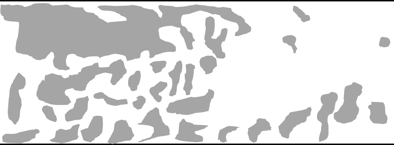
Many of the experimental photographs of Lindgren (Reference Lindgren1959a) show that chaotic patches of bentonite suspension appear to be present in the downstream fully developed turbulent pipe flows at  $Re=3740$ and
 $7650$, see figure 1. He only made this observation in passing without giving any further comments, and no follow-up study of this phenomenon has been reported over the past six decades. Intuitively, one would think that these are perhaps related to coherent structures in turbulent flow such as the large-scale motion (LSM) seen in boundary layers; or perhaps, these are the turbulent–turbulent spots discovered recently from the inner region of the flat-plate turbulent boundary layer (Wu et al. Reference Wu, Moin, Wallace, Skarda, Adrián and Hickey2017). Boundary-layer LSMs are ramp-like, and the turbulent–turbulent spots in Wu et al. are inside the inner layer
 $(y^{+}<100)$ of the boundary layer whereas the ‘turbulent scalar patch’ observed by Lindgren (figure 1) from fully developed turbulent flow occupies the entire pipe cross-section and seems to be plug like. It turns out, based on the present study, that even though the chaotic patches of bentonite suspension reside in turbulent flow, they are most likely initiated by the formation of transitional–turbulent spots in the breakdown of the laminar flow. In other words, they are the passive scalar field’s memory of the far upstream transition.
Sketch illustrating the passive scalar visualization of Lindgren (Reference Lindgren1959a) using bentonite suspensions in turbulent pipe flow at  $Re=3740$ and 7650. Flow is from left to right. The large chaotic blob is puzzling, which was commented on in passing by Lindgren as ‘turbulent patches appear to be present in fully developed turbulent flows’.

To assess whether the flow downstream is indeed fully developed turbulence, the rate of dissipation of turbulent kinetic energy,  $\unicode[STIX]{x1D700}$, has been evaluated over a range of axial locations and compared to that extracted from an axially periodic, fully developed turbulent pipe simulation at the same Reynolds number. The dissipation data agree well. More interestingly, the profiles sampled at late transition stations display significant overshoot in comparison to the fully developed turbulent profile. The mechanism behind such an overshoot is addressed.
Because the formation of transitional–turbulent spots has been identified here as the root cause of the turbulent scalar patch, it is rather natural to contrast the structural composition of spots in pipe flow with that of transitional–turbulent spots in a boundary layer. Examination of the three-dimensional vortex structures in pipe flow reveals that the core region is populated by forward hairpin vortices whereas, quite surprisingly, the near-wall region is dominated by reverse hairpin vortices. It is well known on the other hand that the boundary-layer transitional–turbulent spot is essentially a dense forest of forward hairpins whose heads lie away from the wall and downstream of the legs (Wu & Moin Reference Wu and Moin2009, Reference Wu and Moin2010). On re-examining Case S5R8 data of Wu et al. (Reference Wu, Moin, Adrian and Baltzer2015) with the circumferential-mode inlet disturbance, we find that the mature turbulent spots are also composed of dual-type hairpin vortices. The dense population of reverse hairpin vortices in pipe turbulent spots turns out to be associated with high-speed streaks introduced unintentionally from the two different synthetic inlet conditions. This is somewhat analogous to the concentrated forward hairpin vortices found on the low-speed streaks behind a synthetic jet issuing from a wall slot into a laminar boundary layer (Acarlar & Smith Reference Acarlar and Smith1987; Sau & Mahesh Reference Sau and Mahesh2008). Of course, the Acarlar–Smith case is a reduced scenario of the more general idea of forward hairpin packets forming around low-speed fluid on the side away from the wall and reverse hairpins forming around high-speed fluid on the side close to the wall. For example, in fully turbulent flows, forward hairpins form around local ejections of low-speed flow (Zhou et al. Reference Zhou, Adrian, Balachandar and Kendall1999; Adrian, Meinhart & Tomkins Reference Adrian, Meinhart and Tomkins2000); in homogeneous shear flows (Rogers & Moin Reference Rogers and Moin1987; Vanderwel & Tavoularis Reference Vanderwel and Tavoularis2011), forward hairpins occur around low-speed flow, and reverse hairpins occur around high-speed flow.
After explaining the formation of reverse hairpin vortices in pipe transition, we attempt to quantify their number density. Quantification of hairpin vortices, either forward or reverse, has remained an unsolved challenging problem primarily because it is difficult to auto-select such regular structures among a sea of other irregular structures. The fact that the hairpins tangle with each other and with other structures poses another difficulty for auto-selection. Here, we take an indirect approach towards the quantification of reverse hairpin vortices in pipe flow. We found that the occurrence of negative skin friction is almost always associated with the head element of a reverse hairpin vortex in both transitional and turbulent pipe flows, see also Chin et al. (Reference Chin, Monty, Chong and Marusic2018), Jalalabadi & Sung (Reference Jalalabadi and Sung2018) and Wu, Cruickshank & Ghaemi (Reference Wu, Cruickshank and Ghaemi2020). Thus, the number density of pipe flow reverse hairpin vortices is estimated using the number density of negative skin-friction patches, with the understanding that this is an under-estimation since not every reverse hairpin is associated with a negative skin-friction patch at each instant.
2 Previous simulations of transition in pipe flow
To this day, numerical simulation of pipe flow transition has been confined to the temporal approach with an axially periodic domain. Early temporal simulations of pipe flow transition often used very short pipe lengths  $({\sim}10R)$. Those studies, together with advances in related state theory of viewing pipe flow as a dynamic system, were summarized in Eckhardt et al. (Reference Eckhardt, Schneider, Hof and Westerweel2007) and Mullin (Reference Mullin2011).
The first temporal simulation of pipe transition that was capable of representing turbulent spots was reported by Leonard (Reference Leonard1983). The turbulent spots simulated by Shan et al. (Reference Shan, Ma, Zhang and Nieuwstadt1999), at  $Re=2200$ and 5000 in a pipe
 $32\unicode[STIX]{x03C0}R$ long, were initiated with localized blowing and suction. Several connections were made between their numerical results and the experiment of Wygnanski & Champagne (Reference Wygnanski and Champagne1973). Priymak & Miyazaki (Reference Priymak and Miyazaki2004) used a similar axially periodic pipe length, but ran their temporal simulations for much longer, up to
 $t=4000R/V$ at
 $Re=2300$. They showed that the centreline velocity values before the arrival and after the passage of spots are far from the constant
 $2V$ expected from a fully developed laminar pipe flow, reflecting a quantitative deficiency in this simulation approach with short domains. Willis & Kerswell (Reference Willis and Kerswell2007) also used an axially periodic domain
 $32\unicode[STIX]{x03C0}R$ long and generated their turbulent spots with a localized body force term for
 $1500<Re<2250$. Their results agreed with the exponential scaling of spot life time found experimentally by Eckhardt et al. (Reference Eckhardt, Schneider, Hof and Westerweel2007). Further, they re-interpreted some of the earlier temporal simulations performed on a
 $10R$ long periodic domain and found that those results also agreed with the exponential scaling of life time.
Shimizu & Kida (Reference Shimizu and Kida2009) perturbed the fully developed laminar profile globally across a  $16\unicode[STIX]{x03C0}R$ long axially periodic pipe at
 $Re=3000$. The total integration time was
 $t=3000R/V$, and the spot evolved to an equilibrium state with a length of
 $11\unicode[STIX]{x03C0}R$. Their results agree with the earlier experimental observation by Bandyopadhyay (Reference Bandyopadhyay1986) that the Kelvin–Helmholtz instability related to the vortex sheet inside the spot is an important factor in sustaining the equilibrium spot, see also Duguet & Willis (Reference Duguet, Willis and Kerswell2010). Moxey & Barkley (Reference Moxey and Barkley2010) applied the periodic boundary condition in the axial direction of a pipe up to
 $250R$ in length with an initial condition of a space-filling fully turbulent field at
 $Re=3000$. Temporal development of the flow was then followed at different values of the Reynolds number. It was observed that for
 $2250<Re<2300$, spots are localized and long-time transient; for
 $2300<Re<2600$, pipe-length-filling laminar and turbulent states alternate in time, exhibiting intermittency; for
 $Re>2600$, there was continuous turbulence throughout the pipe without turbulent spots. These observations have been supported by the related temporal pipe transition simulations of Avila et al. (Reference Avila, Moxey, de LOZAR, Avila, Barkley and Hof2011) and Barkley et al. (Reference Barkley, Song, Mukund, Lemoult, Avila and Hof2015).
Although fully developed turbulent pipe flow is homogeneous in the axial direction, laboratory experiments such as those of Reynolds (Reference Reynolds1883) and Lindgren (Reference Lindgren1959a,Reference Lindgrenb,Reference Lindgrenc) are not, owing to flow development in the entrance/transitional region. The axially periodic boundary condition was finally removed in the direct numerical simulation (DNS) of pipe transition performed by Wu et al. (Reference Wu, Moin, Adrian and Baltzer2015). Their pipe length was  $250R$, and the Reynolds number ranged from 6000 to 8000. The pipe inlet flow was the parabolic laminar profile superimposed with a thin numerical wire ring in which a turbulent pipe velocity profile was imposed, corresponding to a localized, weak circumferential-mode inflow disturbance. The computed friction factor
 $f$ agreed with the fully developed laminar solution prior to breakdown, and it also agreed with Moody’s correlation downstream of transition. The observed laminar flow breakdown process involved the generation of turbulent spots through the formation of hairpin packets out of the debris of decaying inlet disturbance. This process was broadly analogous to that of boundary-layer bypass transition in the narrow sense (Wu et al. Reference Wu, Moin, Wallace, Skarda, Adrián and Hickey2017), and it is also in qualitative agreement with experimental observations of transition in pipes caused by very weak finite amplitude upstream perturbations (Peixinho & Mullin Reference Peixinho and Mullin2007). The issue of structural composition of mature turbulent spots was not explored in Wu et al. (Reference Wu, Moin, Adrian and Baltzer2015).
3 Simulation method
In this study the Reynolds number is super-critical,  $Re=6500$, and the pipe length is
 $500R$. The radius normalized by the viscous length scale is
 $R^{+}=Ru_{\unicode[STIX]{x1D70F}}/\unicode[STIX]{x1D708}=215$ in the region of fully developed turbulent flow, where
 $u_{\unicode[STIX]{x1D70F}}$ is the frictional velocity.
The governing equations are the continuity and the Navier–Stokes equations for incompressible flow in cylindrical coordinates. The computer program is based on the fractional-step method, and the details of the numerical scheme were described by Pierce & Moin (Reference Pierce and Moin2001, Reference Pierce and Moin2004) in their large-eddy simulation of combustion in a co-axial jet combustor. That configuration is degenerated into a spatially developing circular pipe. The computational mesh size for the  $500R$ long pipe is
 $16\,384\times 200\times 512$ in the axial, radial and azimuthal directions, respectively. Grid resolutions measured using the computed Kolmogorov length scale
 $\unicode[STIX]{x1D702}=(\unicode[STIX]{x1D708}^{3}/\unicode[STIX]{x1D700})^{1/4}$ were evaluated at two selected axial locations,
 $z=60R$ (late transition stage) and
 $z=450R$ (fully developed turbulent state). In both regions of the pipe,
 $\unicode[STIX]{x0394}z$ is less than
 $5\unicode[STIX]{x1D702}$, whereas
 $\unicode[STIX]{x0394}r$ is always less than
 $1.5\unicode[STIX]{x1D702}$. Grid resolution along the circumferential direction was conservatively evaluated using the product of radius
 $R$ and
 $\unicode[STIX]{x0394}\unicode[STIX]{x1D703}$, and is always less than
 $2\unicode[STIX]{x1D702}$. Time step remains a constant
 $\unicode[STIX]{x0394}t=0.005R/V$. During the computation, the Courant–Friedrichs–Lewy (CFL) number is always less than 0.4. An overbar denotes time averaging, superscript + denotes normalization by the friction velocity
 $u_{\unicode[STIX]{x1D70F}}$ for velocity, and by the viscous length scale
 $\unicode[STIX]{x1D708}/u_{\unicode[STIX]{x1D70F}}$ for distance. The Poisson equation for pressure is solved using Fourier and cosine transforms along the azimuthal and axial directions, respectively.
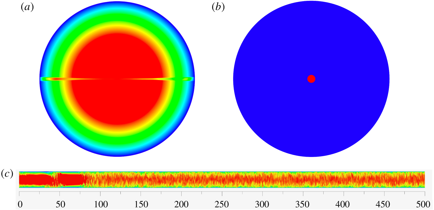
The inlet base flow has the fully developed parabolic laminar velocity profile everywhere, except inside a narrow  $(3^{\circ })$ wedge (figure 2a). Within the wedge, the exact laminar parabolic velocity profile is replaced by the time-dependent, fully developed turbulent pipe DNS velocity field at
 $Re=5300$ (Wu & Moin Reference Wu and Moin2008; Wu Reference Wu2017), mimicking to some extent the narrow turbulent wake behind a thin splitter plate. This type of radial-mode inlet disturbance is broadly in line with the parallel-edge disturbance used by Lindgren (Reference Lindgren1959a). This inlet design is also useful so that we can address the question regarding the dependence of DNS results on the nature of the inlet disturbance (circumferential mode in Wu et al. Reference Wu, Moin, Adrian and Baltzer2015 versus the present radial mode). Mass flow rate over the inlet plane is kept constant with time. In the new, radial-mode disturbance simulation, a numerical dye (represented by symbol
 $\unicode[STIX]{x1D719}$) is also added (figure 2b) by introducing a passive scalar at the inlet plane in a region very close to the pipe axis
 $(0\leqslant r\leqslant 0.05)$, similar to the syringe needle injection of dye by Reynolds. The scalar satisfies the adiabatic, zero-flux boundary condition on the pipe wall. Molecular Prandtl number for the passive scalar is chosen as
 $1$ in the hope that the scalar motion resembles momentum diffusion and convection.
Illustration of the present simulation design of pipe transition excited by a radial-mode inlet disturbance using two-dimensional contours of axial velocity and passive scalar at  $t=176\,000\unicode[STIX]{x0394}t$: (a)
 $u_{z}/V$ over the inlet plane, within the
 $3^{\circ }$ numerical wedge the laminar parabolic velocity profile is replaced with a time-dependent turbulent pipe flow profile; (b)
 $\unicode[STIX]{x1D719}$ over the inlet plane, centreline dye injection is mimicked by prescribing
 $\unicode[STIX]{x1D719}=1$ for
 $r\leqslant 0.05R$ and
 $\unicode[STIX]{x1D719}=0$ otherwise.
 $\unicode[STIX]{x1D719}=0.00475$ is the mean over the inlet plane; (c)
 $u_{z}/V$ over a plane (radial dimension enlarged by a factor of 10) passing through the pipe centreline, a turbulent spot within
 $30R<z<60R$ can be inferred from the contours. For axial velocity, blue and red colours correspond to
 $u_{z}/V\leqslant 0$ and
 $u_{z}/V\geqslant 1.4$, respectively.

4 Turbulent scalar flashes in fully developed turbulent pipe flow
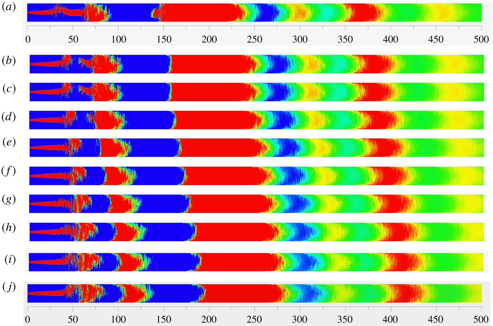
Under the current inlet condition shown in figure 2(b) and with the imposed adiabatic zero-flux boundary condition, the flow-averaged passive scalar value over the inlet plane is  $\overline{\unicode[STIX]{x1D719}}_{z=0}=\int _{0}^{R}2\unicode[STIX]{x03C0}ru_{z}\unicode[STIX]{x1D719}\,\text{d}r/V\unicode[STIX]{x03C0}R^{2}\simeq 0.00475$, corresponding to the yellow colour in the two-dimensional contour plots of
 $\unicode[STIX]{x1D719}$ over the side view planes in figure 3. A segmented distribution of passive scalar along the axial direction is evident, and the segments migrate downstream with the flow. The segmented distribution is counter-intuitive because one expects turbulence in the fully developed flow region to rapidly mix the scalar field. This expectation also constitutes the basis of several flow visualization techniques, e.g. detection of LSM in turbulent flows via smoke injection. It is quite obvious one only needs to identify the cause of the first two leftmost (chaotic) scalar segments for the purpose of understanding the nature of the scalar segmentation throughout the pipe.
Contours of scalar  $\unicode[STIX]{x1D719}$ over a plane (radial dimension enlarged by a factor of 10) passing through the pipe centreline at 10 consecutive instants: (a)
 $t=215\,000\unicode[STIX]{x0394}t$; (b)
 $216\,000\unicode[STIX]{x0394}t$; (c)
 $217\,000\unicode[STIX]{x0394}t$; (d)
 $218\,000\unicode[STIX]{x0394}t$; (e)
 $219\,000\unicode[STIX]{x0394}t$; (f)
 $220\,000\unicode[STIX]{x0394}t$; (g)
 $221\,000\unicode[STIX]{x0394}t$; (h)
 $222\,000\unicode[STIX]{x0394}t$; (i)
 $223\,000\unicode[STIX]{x0394}t$; (j)
 $224\,000\unicode[STIX]{x0394}t$. Blue and red colours correspond to
 $\unicode[STIX]{x1D719}\leqslant 0.0035$ and
 $\unicode[STIX]{x1D719}\geqslant 0.0055$, respectively. Yellow colour corresponds to approximately
 $0.0045\leqslant \unicode[STIX]{x1D719}<0.0050$. The figure demonstrates that scalar segmentation actually begins with the formation of a transitional–turbulent spot. Here, the appearance of the dark blue patch with low scalar value at
 $z\approx 50R$ and
 $t=217\,000\unicode[STIX]{x0394}t$ in (c) is due to the strong mixing effect of the turbulent spot in
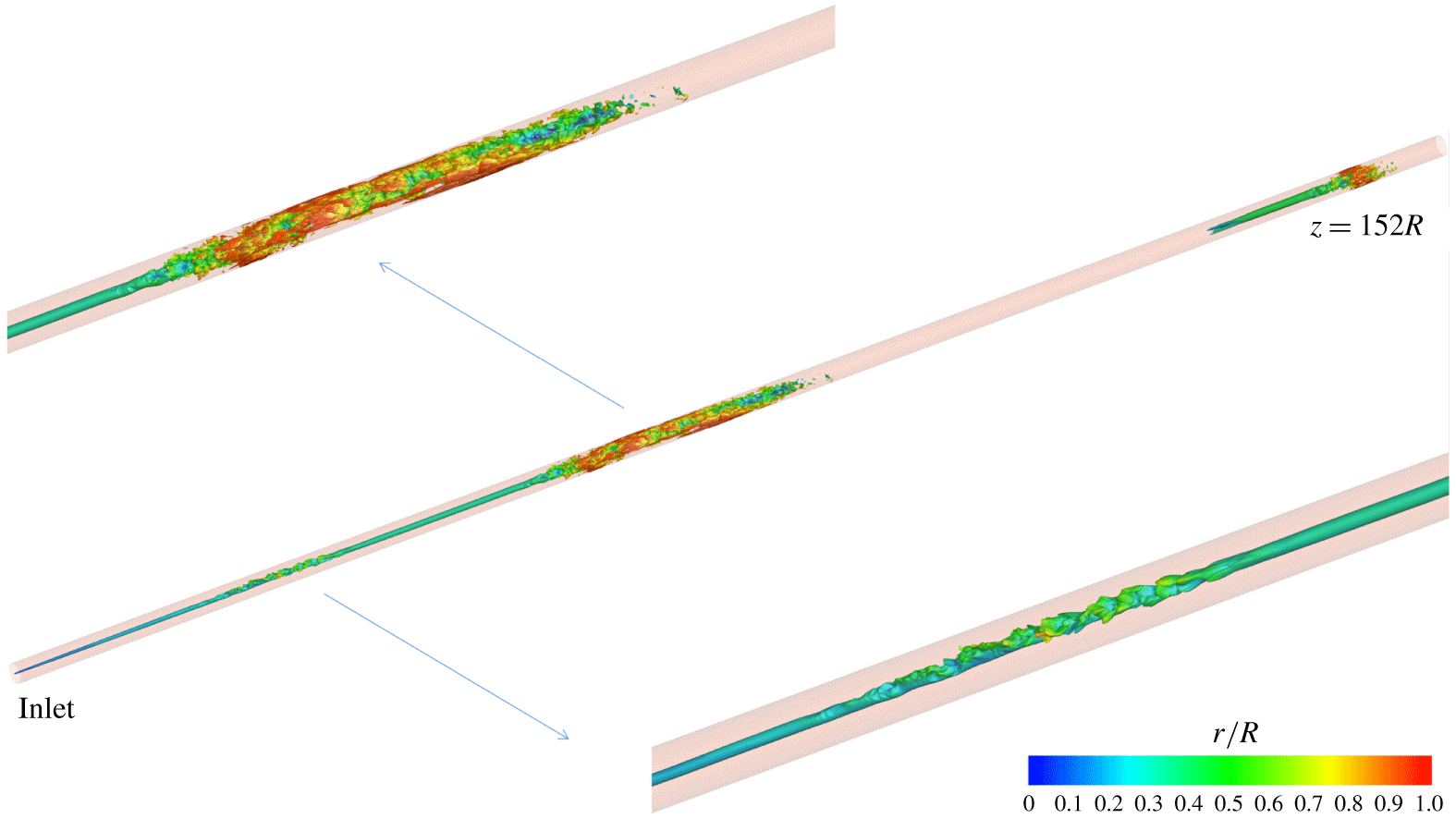
 $25R<z<50R$, which absorbs a large portion of the upstream scalar supply to the fluid immediately downstream of the spot. This particular turbulent spot is the same as that shown in the lower inset of figure 4. By the instant
 $t=224\,000\unicode[STIX]{x0394}t$, the dark blue patch has migrated to the downstream region
 $85R<z<105R$ in (j).

In the early transitional region  $0<z<25R$, all the panels in figure 3 are similar: since the local flow is mostly laminar, the smooth narrow red coloured scalar stream along the centreline is directly from the injection on the inlet plane over
 $0\leqslant r\leqslant 0.05$. See also figure 4 in the same region between the inlet and the first spot.
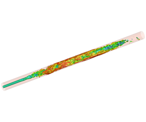
Isosurfaces of passive scalar  $\unicode[STIX]{x1D719}=0.00475$ at
 $t=215\,000\unicode[STIX]{x0394}t$. The colour of a point on the isosurface represents its radial position
 $r/R$.

The dark red coloured chaotic scalar field within  $25R<z<50R$ in figures 3(a) and 3(b) is the result of the first transitional–turbulent spot shown in the lower inset of figure 4. The strong turbulent mixing capability of the transitional–turbulent spot ‘consumes’ a portion of the scalar flow rate supply coming from the inlet injection stream along the centreline. This reduces the supply of scalar flow rate to the fluid immediately downstream of the spot, resulting in a small blue patch with low value of
 $\unicode[STIX]{x1D719}$ in figure 3(c) at
 $z\approx 50R$. In this way, the first pair of red–blue chaotic scalar patches is formed, which propagates downstream with time as shown in figures 3(d) to 3(j).
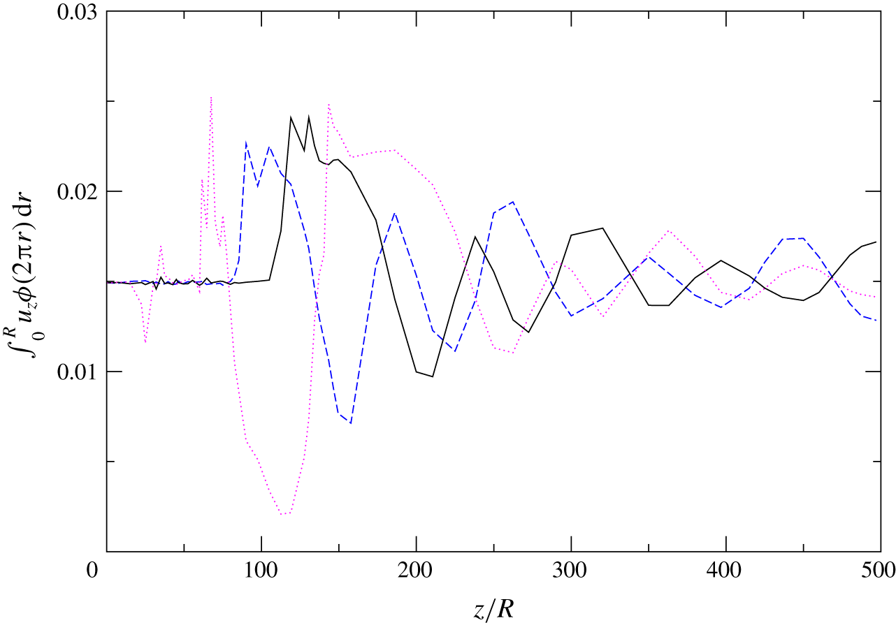
This understanding is reinforced by plotting the instantaneous scalar flow rate integrated over each axial cross-section,  $\int _{0}^{R}u_{z}\unicode[STIX]{x1D719}(2\unicode[STIX]{x03C0}r)\,\text{d}r$, as a function of the axial distance in figure 5. It is obvious the scalar flow rate, hence the cross-sectional mean
 $\overline{\unicode[STIX]{x1D719}}(z)$, is non-constant as soon as the laminar flow starts to break down. At
 $=205\,000\unicode[STIX]{x0394}t$ (solid line), the scalar flow rate remains nearly constant until
 $z\approx 110R$ since the flow velocity field remains mostly laminar in this region. The minor peaks and valleys on the solid line in this range are likely due the transport events of early transitional structures such as discrete hairpin packets. The zig-zag characteristics of the scalar flow rate profiles correspond to the segmented contours shown in figure 3. In particular, the profile at
 $t=215\,000\unicode[STIX]{x0394}t$ (dotted line) exhibits a sharp spike followed immediately by a deep valley within the axial range
 $60R<z<140R$. Note this instant is the same as that of figure 3(a). The spike appearing in
 $60R<z<80R$ is the direct result of the transitional–turbulent spot shown earlier in the upper inset of figure 4, which ‘blocks’ the upstream scalar supply to the fluid behind the spot, resulting in the deep valley in
 $80R<z<140R$.
Variation of scalar flow rate  $\int _{0}^{R}u_{z}\unicode[STIX]{x1D719}(2\unicode[STIX]{x03C0}r)\,\text{d}r$ as a function of axial distance. Dotted line:
 $t=215\,000\unicode[STIX]{x0394}t$ corresponding to figure 3(a). The peaks within
 $60<z/R<80$ are related to the first red patch in figure 3(a) caused by the turbulent spot in figures 4 and 11, whereas the deep valley around
 $z/R=110$ is related to the first deep blue patch in figure 3(b) caused by the turbulent spot’s ‘consumption of’ the upstream scalar supply. Solid line:
 $t=205\,000\unicode[STIX]{x0394}t$; dashed line:
 $t=195\,000\unicode[STIX]{x0394}t$. The zig-zag pattern of the scalar flow rate reflects the segmented nature of the scalar distribution along the pipe axis.

Goto, Kida & Fujiwara (Reference Goto, Kida and Fujiwara2011) analysed the flow visualization technique using reflective flakes, whose pattern in an image, under a set of idealized conditions, should stem from their non-uniform orientation rather than their spatial accumulation. In their model, Goto et al. assumed that the flakes are so diluted that interactions between them are negligible, and the spatial distribution of flakes always remains uniform in a Newtonian incompressible fluid. They admitted that their model cannot deal with the effects of flake accumulation. Lindgren (Reference Lindgren1953) reported that his bentonite suspensions had an initially uniform weight concentration from 0.08 % to 1 %, and he observed that when the bentonite concentration exceeded approximately 2 % the suspension behaved like a thixotropic gel. He also admitted that even his more diluted suspensions cannot be expected to behave exactly like Newtonian fluids. Lindgren further pointed out that these anomalous properties of the suspensions must be considered in connection with his flow visualization images. Even though Lindgren’s bentonite suspensions had an initially uniform concentration, the strong turbulent mixing capability of the transitional–turbulent spot during pipe transition would block a portion of the bentonite supply coming from the upstream, resulting in a local accumulation and high concentration of the suspensions. This would in turn render the assumptions of Goto et al. (Reference Goto, Kida and Fujiwara2011) invalid. Note that this ‘blocking’ effect by turbulent spot is operative regardless of whether the upstream flow has uniform scalar concentration (as in Lindgren (Reference Lindgren1959a)) or non-uniform scalar concentration (as in the present flow). Therefore, it is quite likely that the plug-like patch sketched in figure 1 is a manifestation of non-uniform scalar concentration.
Thus, it is reasonable to suspect that the ‘turbulent bentonite suspension patches’ observed by Lindgren (Reference Lindgren1959a) in the fully turbulent pipe flow region are due to scalar field segmentation, which in turn originates from the formation of transitional–turbulent spots during pipe transition. Such turbulent scalar flashes carry a surprisingly persistent memory of transition events that occurred far upstream.
5 Overshoot of turbulence statistics in the late transition region
Given the segmented nature of the scalar field presented in figure 3, it is necessary to ask if the turbulent velocity field in the range  $200R<z<500R$ (figure 2c) is indeed fully developed pipe flow turbulence.
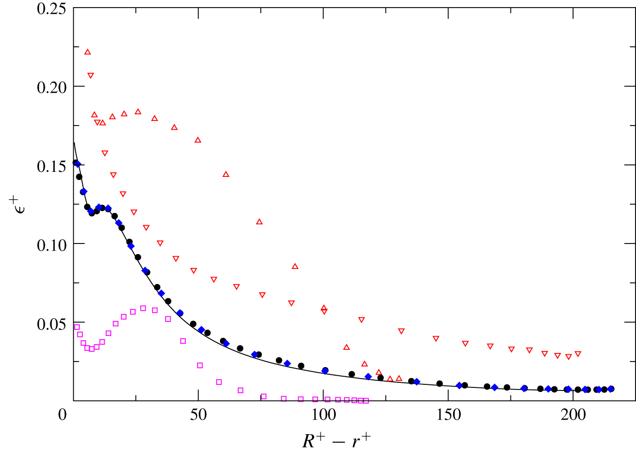
Figure 6 shows the radial profiles of normalized rate of viscous dissipation of turbulent kinetic energy  $\unicode[STIX]{x1D700}^{+}=\unicode[STIX]{x1D700}/(u_{\unicode[STIX]{x1D70F}}^{4}/\unicode[STIX]{x1D708})$ as a function of
 $R^{+}-r^{+}$. In the figure, the two profiles sampled at
 $z=225R$ and
 $400R$ collapse over the profile extracted from an auxiliary simulation (solid line). That auxiliary DNS computed fully developed turbulent pipe flow at
 $Re=6500$ using the conventional axially periodic condition with a
 $30R$ long pipe on a mesh of
 $2048\times 256\times 512$. According to Chin et al. (Reference Chin, Ooi, Marusic and Blackburn2010), this domain length should be sufficient. Radial profiles of the mean axial velocity and Reynolds stresses at
 $z=225R$ and
 $400R$ (not shown) were also cross-checked against those sampled from the auxiliary DNS. Excellent agreement among the three sets of statistics confirms that the segmented scalar field indeed exists in a velocity field of fully developed pipe flow turbulence after transition.
Rate of dissipation of turbulent kinetic energy  $\unicode[STIX]{x1D716}^{+}=\unicode[STIX]{x1D716}/(u_{\unicode[STIX]{x1D70F}}^{4}/\unicode[STIX]{x1D708})$ at
 $Re_{D}=6500$. Solid line: present auxiliary DNS with the conventional axially periodic boundary condition on a
 $30R$ long fully developed turbulent pipe flow. Symbols: the present spatially developing simulation. Circle:
 $z=400R$; diamond:
 $z=225R$; nabla:
 $z=82.5R$; triangle:
 $z=30R$; box:
 $z=15R$. Note the two profiles in the late transitional zone overshoot the fully developed turbulent profiles.

Comparison of the  $\unicode[STIX]{x1D700}^{+}$ profiles during and after transition in figure 6 suggests that second-order turbulence statistics collected in the late transitional region
 $(z=30R,82.5R)$ sharply overshoot the values observed in the fully developed turbulent region. Overshoot is observed regardless of whether the profiles are normalized by inner or outer variables. Inner variables such as
 $u_{\unicode[STIX]{x1D70F}}$ vary with axial distance in pipe flow during transition whereas outer variables
 $V$ and
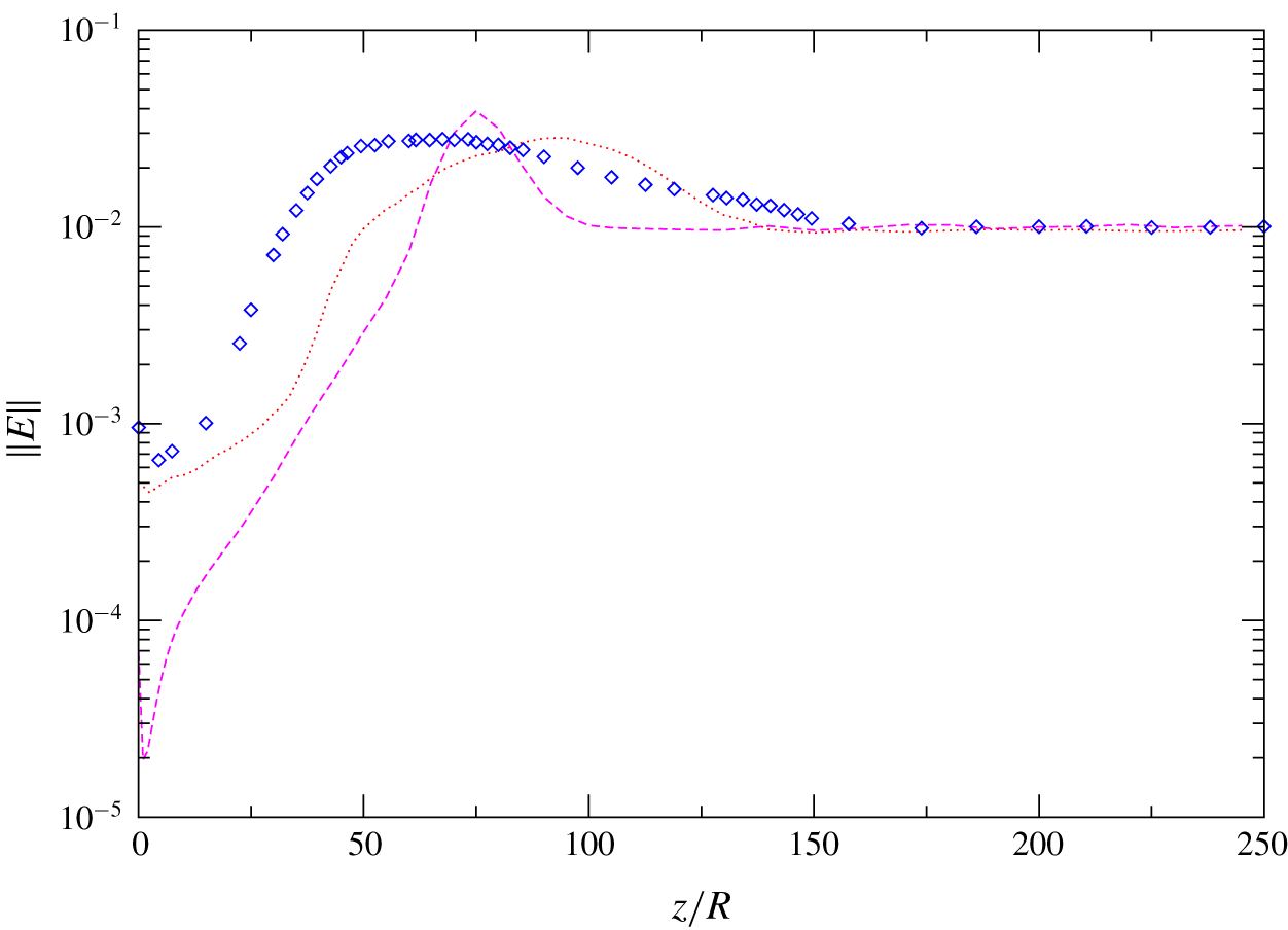
 $R$ are constants. Figure 7 shows the mean turbulent kinetic energy integrated over the pipe cross-section as a function of axial distance,
 $\Vert E\Vert =\int _{0}^{R}(u_{z,rms}^{\prime 2}+u_{\unicode[STIX]{x1D703},rms}^{\prime 2}+u_{r,rms}^{\prime 2})r\,\text{d}r/(R^{2}V^{2})$, for the present case and Cases S4R6 and S5R8 of Wu et al. (Reference Wu, Moin, Adrian and Baltzer2015). Subscript
 $_{rms}$ denotes root-mean-square value. In each of the three types of pipe flow the energy norm overshoots the respective constant value it achieves in the region of fully developed flow, irrespective of the type of inflow perturbation (circumferential mode in Wu et al. Reference Wu, Moin, Adrian and Baltzer2015 versus the present radial mode). Note that the inlet disturbance ring in Case S4R6 is placed at
 $0.4R<r<0.42R$, further away from the wall compared to Case S5R8 (disturbance ring located at
 $0.9R<r<0.915R$) and the present flow. In the latter two cases, over the inlet plane at least part of the near-wall flow is directly perturbed whereas in Case S4R6 the near-wall flow remains virtually laminar even for a considerable distance downstream of the inlet.
Energy norm  $\Vert E\Vert =\int _{0}^{R}(u_{z,rms}^{\prime 2}+u_{\unicode[STIX]{x1D703},rms}^{\prime 2}+u_{r,rms}^{\prime 2})r\,\text{d}r/(R^{2}V^{2})$ as a function of axial distance
 $z$ in the transitional region. Diamond: present flow with radial-mode inlet disturbance at
 $Re_{D}=6500$; dashed line: Case S4R6 in Wu et al. (Reference Wu, Moin, Adrian and Baltzer2015) with circumferential-mode inlet disturbance at
 $Re_{D}=6000$, ring position at
 $0.4R<r<0.42R$; dotted line: Case S5R8 in Wu et al. (Reference Wu, Moin, Adrian and Baltzer2015) with circumferential-mode inlet disturbance at
 $Re_{D}=8000$, ring position at
 $0.9R<r<0.915R$. It is seen that the rate of energy growth during the late stage of transition is similar between the present flow and Case S5R8 in which at least part of the near-wall flow is perturbed at the inlet. The energy norm in Case S4R6 is lower initially because the inlet disturbance is placed further away from the wall.

Overshoot of turbulent statistics during late transition may be a distinct feature of internal transitional flows where the Reynolds number is constant with respect to axial distance. For external transitional flows such as the zero-pressure-gradient smooth flat plate boundary layer (ZPGSFPBL), it is unclear whether such distinct overshoot can be convincingly identified. We examined the local peak values of the streamwise turbulence intensity as a function of the momentum-thickness Reynolds number  $Re_{\unicode[STIX]{x1D703}}$ in the ZPGSFPBL of Wu et al. (Reference Wu, Moin, Wallace, Skarda, Adrián and Hickey2017), together with the low Reynolds number turbulent ZPGSFPBL experimental data of Purtell, Klebanoff & Buckley (Reference Purtell, Klebanoff and Buckley1981) and Erm & Joubert (Reference Erm and Joubert1991). No convincing overshoot could be unequivocally identified from those boundary-layer data as compared to the distinct pipe flow overshoot shown in figures 6 and 7.
6 Explanation of the observed statistics overshoot
Here we give an account, from both statistical and structural viewpoints, of the factors contributing to the statistics overshoot during pipe transition.
We start by examining energy spectra to see if we can identify the range of scales associated with the overshoot. To compute frequency spectra, the instantaneous velocity, pressure and scalar data at  $z=30R,60R,90R,350R,400R$ and
 $450R$ were saved at each time step continuously for a duration of
 $50\,000\unicode[STIX]{x0394}t$. The first three axial locations are in the transitional region, and the rest are in the fully developed turbulent region. At each axial station, two radial locations are chosen,
 $r=0.5R,0.925R$. For each identified axial–radial combination, the data at all the 512 mesh points along the circumferential direction are saved at each time step. Processing of the frequency spectrum data follows the data-windowing procedure described in Choi & Moin (Reference Choi and Moin1990).
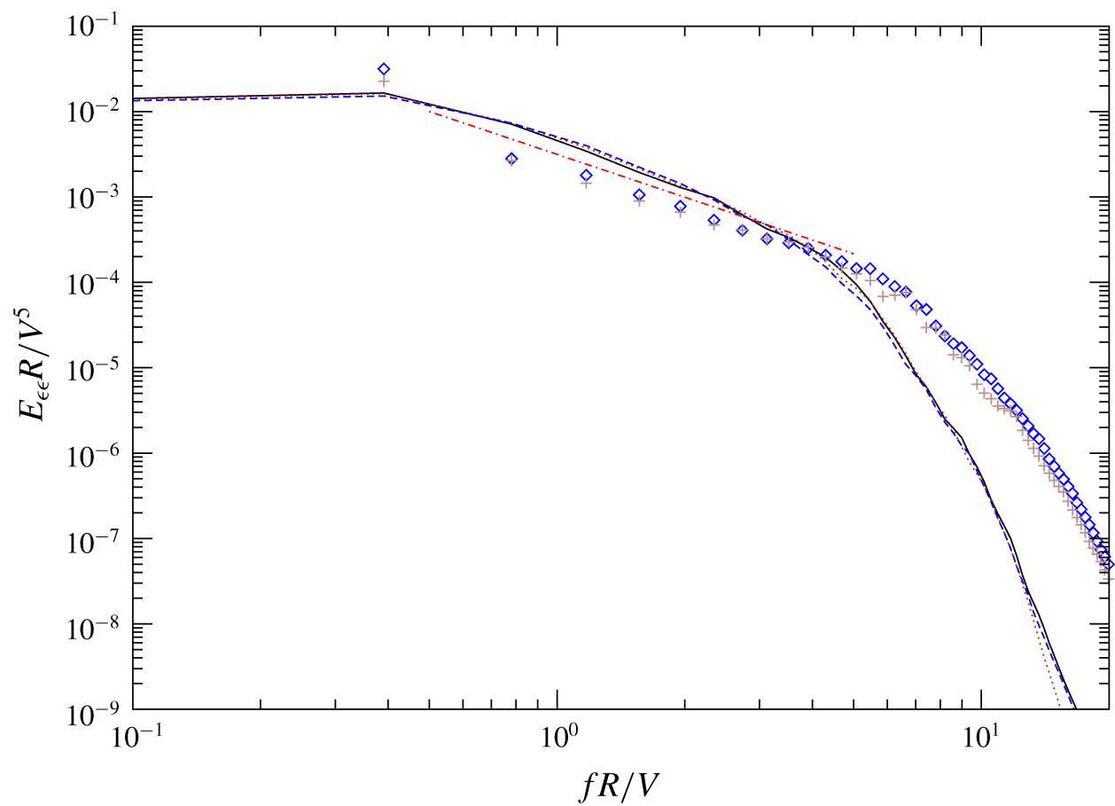
Figure 8 plots the frequency spectrum of the rate of viscous dissipation of turbulent kinetic energy  $E_{\unicode[STIX]{x1D700}\unicode[STIX]{x1D700}}R/V^{5}$ at the radial location
 $r=0.5R$. As expected, the three spectra from the fully developed turbulent zone
 $(z=350R,400R,450R)$ nearly collapse. The two spectra from the late transitional zone
 $(z=60R,90R)$ also collapse onto themselves, but in the mid-to-high frequency range,
 $fR/V>4$, they contribute considerably more to dissipation than the spectra from the fully turbulent zone. Note that the range of transitional flow’s greater contribution to dissipation begins at the end of the
 $-5/3$ range, implying that the overshoot is associated with viscous motion. The dissipation frequency spectra of the flow at the near-wall radial location
 $r=0.925R$ exhibit the same behaviour. This suggests that the higher rates of dissipation that occur at locations in the late transition zone (figure 6) may be associated with the higher spectral energy densities at frequencies past the end of the
 $-5/3$ range.
Frequency spectra of rate of dissipation of turbulent kinetic energy  $E_{\unicode[STIX]{x1D716}\unicode[STIX]{x1D716}}R/V^{5}$ at
 $Re_{D}=6500$. Late transitional region: plus
 $z=60R$; diamond
 $z=90R$; fully developed turbulent region: solid line
 $z=350R$; dotted line
 $z=400R$; dashed line
 $z=450R$. All the profiles are extracted at the radial location
 $r=0.5R$. Dash-dot-dash line:
 $-5/3$ slope. It is evident that the profiles extracted from the late transitional zone have higher mid-to-high frequency content than those from the turbulent zone for the present pipe flow.

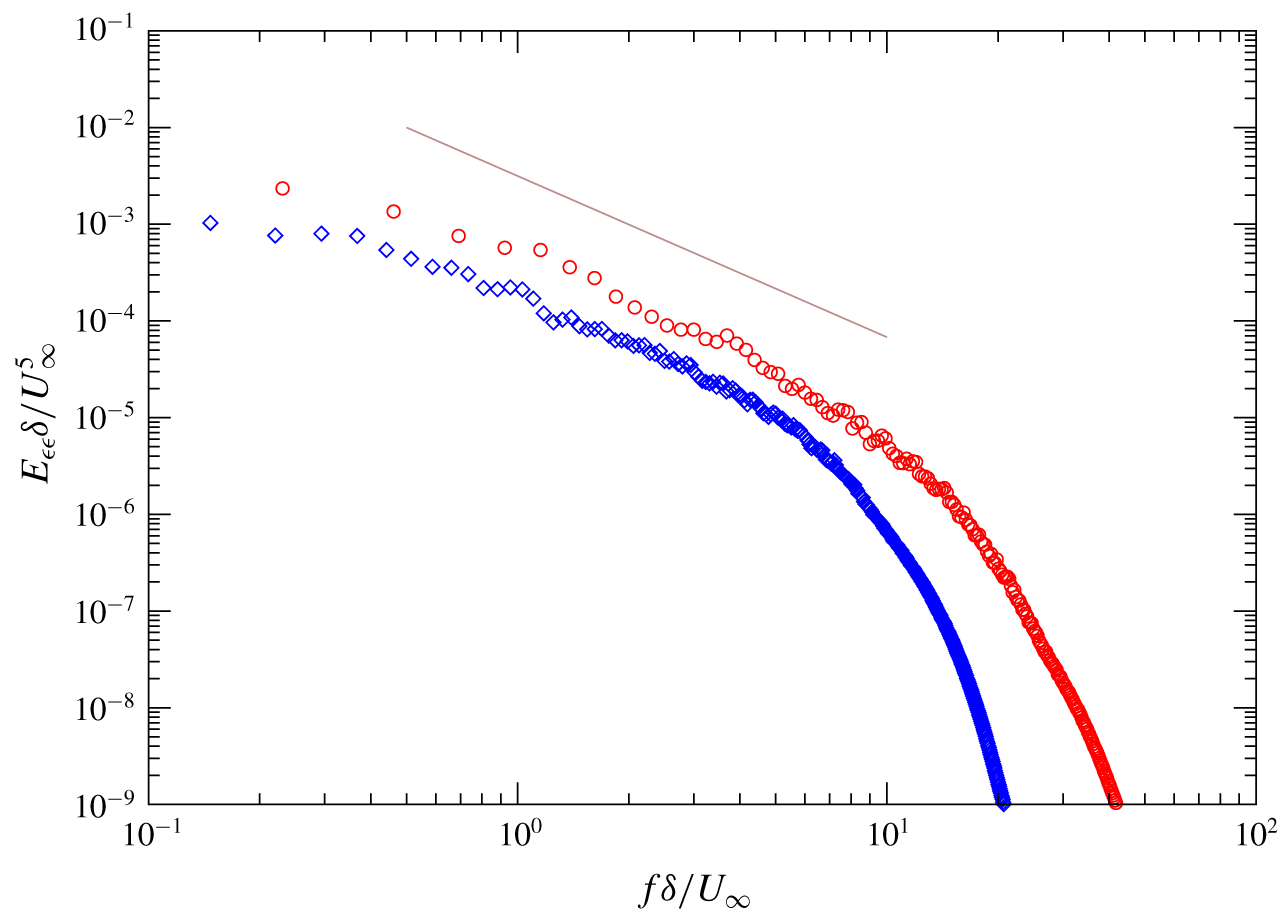
Ordinarily one tends to think that motions in fully developed turbulence possess greater high frequency content than those in transitional turbulence. But this notion is based largely on textbook spectra that show the high frequency part of outer-normalized spectra extending farther with increasing Reynolds number. This is indeed the case for a ZPGSFPBL where the Reynolds number increases with downstream distance. In figure 9, the normalized dissipation frequency spectrum  $E_{\unicode[STIX]{x1D700}\unicode[STIX]{x1D700}}\unicode[STIX]{x1D6FF}/U_{\infty }^{5}$ for the ZPGSFPBL of Wu et al. (Reference Wu, Moin, Wallace, Skarda, Adrián and Hickey2017) is plotted at two streamwise stations:
 $Re_{\unicode[STIX]{x1D703}}=670$ in the late transitional zone and
 $Re_{\unicode[STIX]{x1D703}}=2535$ in the fully turbulent zone. The wall-normal location of each spectrum is
 $y=0.5\unicode[STIX]{x1D6FF}$. It is seen from the figure that the dissipation spectrum for the late transitional zone lies below that for the fully turbulent zone, as expected. Both profiles also exhibit discernible inertial subrange slope.
Frequency spectra for rate of dissipation of turbulence kinetic energy  $E_{\unicode[STIX]{x1D716}\unicode[STIX]{x1D716}}\unicode[STIX]{x1D6FF}/U_{\infty }^{5}$ for the ZPGSFPBL of Wu et al. (Reference Wu, Moin, Wallace, Skarda, Adrián and Hickey2017). Circle:
 $Re_{\unicode[STIX]{x1D703}}=2535$ (fully turbulent region); diamond:
 $Re=670$ (late transitional region). Both profiles are at
 $y=0.5\unicode[STIX]{x1D6FF}$. Straight grey solid line:
 $-5/3$ slope. It is seen that, as expected, the profile in the turbulent region has more high frequency content than that in the late transitional region.

In contrast to the boundary-layer results in figure 9, the dissipation spectrum profiles in figure 8 have a counter-intuitive cross-over where the transition zone spectra overtake the turbulent zone spectra at mid-frequency  $fR/V\sim 4$. Again, one is reminded that the present pipe flow has a constant low Reynolds number independent of either the axial distance or the state of the flow. With this in mind, it is entirely conceivable that the transition region actually does have greater small-scale dissipation than fully turbulent flow because the small vortices in transition are very recently formed and have small diameters with, potentially, sharp edges. In contrast, as they proceed into the fully turbulent flow, viscous diffusion has time to increase their diameters, as do vortex mergers and entanglement. The effect would be like low-pass filtering the fully turbulent spectra, consistent with the behaviour in figure 8.
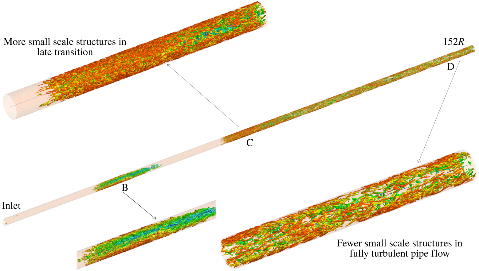
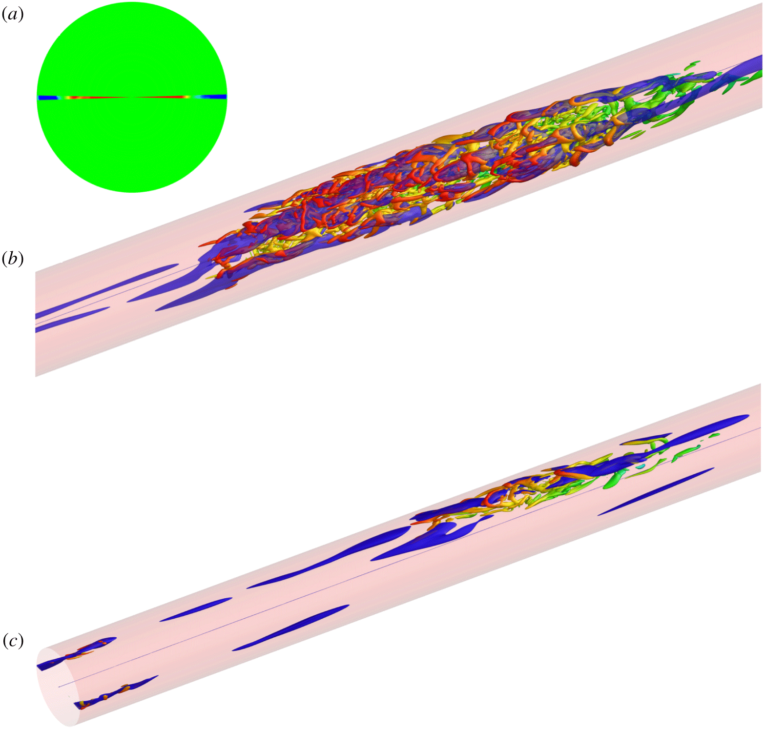
The dissipation spectra of low Reynolds number pipe flow in figure 8 indicate that the spectral density in the mid-to-high frequency range (i.e. after the  $-5/3$ range) is higher in the late transitional zone than in the downstream fully developed turbulent zone. This is further confirmed qualitatively by comparing three-dimensional visualizations of vortex motions inside the two zones. Figure 10 shows the instantaneous isosurfaces of swirling strength
 $\unicode[STIX]{x1D706}_{ci}=1.5$ (Adrian Reference Adrian2007) over
 $0<z<152R$ (approximately the upstream 30 % section of the pipe) at
 $t=176\,000\unicode[STIX]{x0394}t$. Zone B is a transitional–turbulent spot. At this particular time the spot has not yet expanded across over the entire
 $360^{\circ }$ circumference. In late transition (zone B and zone C) the density of small-to-mid-scale vortex structures is much higher than that in the turbulent zone D. The high population of mid-to-small-scale vortex motions during late transition is consistent with overshoot of the turbulence statistics.
Isosurfaces of swirling strength  $\unicode[STIX]{x1D706}_{ci}=1.5V/R$ at
 $t=176\,000\unicode[STIX]{x0394}t$ over the axial region
 $0<z/R<152$. The images demonstrate that there is a higher density of vortices in the late transitional zone (labelled as ‘B’, ‘C’) than in the turbulent zone (labelled as ‘D’) for the present low Reynolds number pipe flow. The colour of a point on the isosurface represents its radial position
 $r/R$, as in figure 4.

Bandyopadhyay (Reference Bandyopadhyay1986) emphasized the importance of tangential shear flow instability (Kelvin–Helmholtz) during pipe transition. He noted that the instability occurs at the upstream interface of the transitional–turbulent spot between the slower near-wall fluid inside the spot and the high-speed laminar fluid near the core. His two-dimensional side view dye images showed a train of three-dimensional wake-like vortices being shed from the upstream interface of the pipe transitional–turbulent spot. See also the numerical work of Duguet & Willis (Reference Duguet, Willis and Kerswell2010). During low Reynolds number pipe transition, it is likely that both the tangential shear flow instability and the wall-turbulence mechanism are at play, whereas in the downstream fully developed turbulent zone only the wall-turbulence mechanism dominates. This difference can explain the higher density of vortical structures observed in the late transitional zone since the tangential shear flow instability is unstable to all wavelengths.
7 Dual-type structural composition of pipe turbulent spots
It has been shown that two pipe flows having substantially different inlet disturbances share qualitatively similar characteristics in terms of overshoot and energy growth rate. It is thus quite natural to explore their eddy structures for similarities or differences during the transition process.
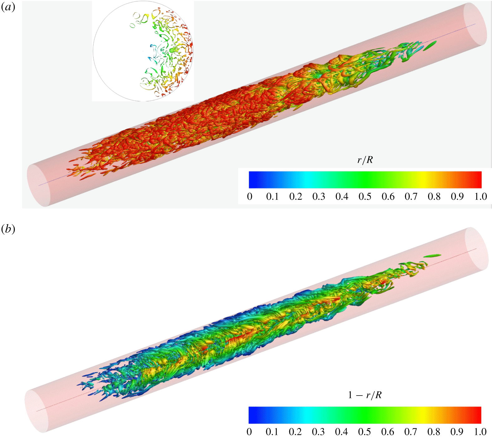
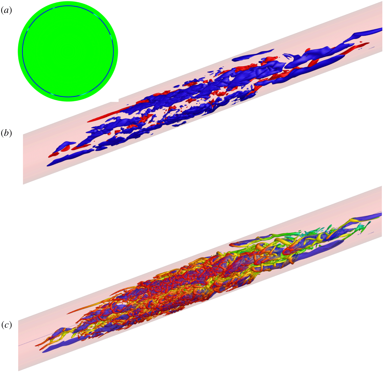
Figure 11(a) visualizes a transitional–turbulent spot from the present case (S7R6P5) at  $t=215\,000\unicode[STIX]{x0394}t$ using isosurfaces of
 $\unicode[STIX]{x1D706}_{ci}=1.5$. It is evident that the near-wall region is dominated by reverse hairpins whose heads are closer to the wall and upstream of the legs. Reverse hairpins are observed, in general, to dominate the near-wall regions of all early transitional spots in the present pipe flow. For example, the turbulent spot at the earlier instant
 $t=176\,000\unicode[STIX]{x0394}t$ shown in zone B of figure 10 also consists of mostly reverse hairpin vortices in the near-wall region. This is rather surprising since recent measurements of transitional–turbulent spots in pipe flow only indicated the presence of successions of forward hairpin vortices (Winters & Longmire Reference Winters and Longmire2019). However, that study conditionally averaged on strong ejection events, which are known to be characteristic of the upstream ends of forward hairpin packets (Adrian Reference Adrian2007). Hence, their conditional averaging keyed on forward hairpins whereas reverse hairpins generate fourth quadrant (Q4) events (Wallace Reference Wallace2016) that would not be included in the conditional averaging.
Dual structural composition of a turbulent spot ( $14<z/R<36$, see figure 3a) in the pipe flow having radial-mode inlet disturbances. Spot visualized using the isosurfaces of swirling strength
 $\unicode[STIX]{x1D706}_{ci}=1.5V/R$ at
 $t=215\,000\unicode[STIX]{x0394}t$. Inset of (a) is an axial slice of the isosurfaces through the centre of the spot at
 $z/R=25$. It is evident that this mature spot is composed primarily of reverse hairpin vortices in the near-wall region (a) and forward hairpin vortices in the pipe core (b).

While the spot at  $t=215\,000\unicode[STIX]{x0394}t$ does not yet occupy the entire
 $360^{\circ }$ circumference (as indicated by the inset of figure 11a), the view to the core region in figure 11(a) is still blocked by the near-wall reverse hairpins. This is remedied in figure 11(b) where the same turbulent spot is visualized through the unoccupied opening space so that the core becomes visible. Note that the colour scheme in figure 11(b) is changed compared to that in figure 11(a). It is seen that the core region of the turbulent spot consists of mostly forward hairpin vortices, suggesting that the pipe transitional–turbulent spots at
 $Re\sim 6000$ have an interesting dual-type structural composition.
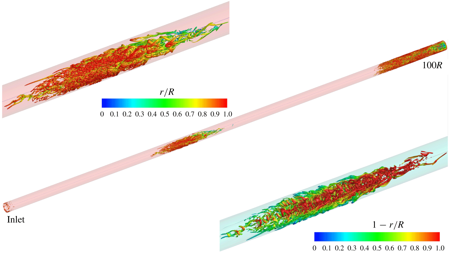
How does such dual-type spot composition found in the present flow under a radial-mode inlet disturbance compare to that in the earlier work of Wu et al. (Reference Wu, Moin, Adrian and Baltzer2015) under a circumferential-type inlet disturbance? Since the structural composition of transitional–turbulent spots was not addressed in Wu et al. (Reference Wu, Moin, Adrian and Baltzer2015), the DNS data fields of Case S5R8 in Wu et al. (Reference Wu, Moin, Adrian and Baltzer2015) are examined in this study. Using isosurfaces of  $\unicode[STIX]{x1D706}_{ci}=2.0V/R$, figure 12 shows a mature turbulent spot from Case S5R8 at
 $t=141\,000\unicode[STIX]{x0394}t$ for the region
 $0<z<100R$. Note that the (near-wall) circumferential-mode inlet disturbance can be seen figure 12. From the upper inset the spot’s near-wall region (reddish colour at large values of
 $r/R$) is dominated by reverse hairpin vortices, similar to that shown in figure 11(a). The lower inset of figure 12 visualizes the core region of the same spot with a changed colour scheme, and it reveals that the pipe core is actually populated by forward hairpins like those in figure 11(b). Thus, transitional turbulent spots in both the radial-mode inlet disturbance Case S7R6P5 and the circumferential-mode inlet disturbance Case S5R8 share the same dual-type structural composition, suggesting that dual composition may be a common phenomenon in pipe transition at
 $6000<Re<8000$. This is both interesting and somewhat puzzling.
Isosurfaces of swirling strength  $\unicode[STIX]{x1D706}_{ci}=2.0V/R$ at
 $t=141\,000\unicode[STIX]{x0394}t$ in Case S5R8 of Wu et al. (Reference Wu, Moin, Adrian and Baltzer2015) over the axial range
 $0<z/R<100$. The circumferential-mode inflow disturbance can be inferred from the isosurfaces near the inlet. It is evident from the upper inset that the near-wall region of the turbulent spot in Case S5R8 is also heavily populated by reverse hairpin vortices, whereas the core region contains mainly forward hairpin vortices (lower inset).

In a ZPGSFPBL, the heads of the hairpin vortices are almost always further away from the wall and downstream of the legs (Wu & Moin Reference Wu and Moin2009). It was reported in Wu et al. (Reference Wu, Moin, Wallace, Skarda, Adrián and Hickey2017) that, for boundary-layer bypass transition in the narrow sense, the process leading to mature transitional–turbulent spots involves a sequential formation of  $\unicode[STIX]{x1D6EC}$-vortices, breakdown near the tip region of the
 $\unicode[STIX]{x1D6EC}$-vortex and creation of hairpin packets, perhaps by the auto-generation mechanism (Zhou et al. Reference Zhou, Adrian, Balachandar and Kendall1999). This process is broadly similar to the secondary instability of boundary-layer natural transition (Herbert Reference Herbert1988; Sayadi, Hamman & Moin Reference Sayadi, Hamman and Moin2013; Zheng, Yang & Chen Reference Zheng, Yang and Chen2016).
8 Explanation for reverse hairpins in transitional–turbulent spots
The phenomenon of reverse hairpin vortices in the near-wall region of transitional–turbulent spots requires explanation. Reverse hairpins have been observed in a few other turbulent flows. Numerical simulations of fully turbulent, wall-free, homogeneous shear flows (HSF) revealed normal hairpins and reverse hairpins occurring with approximately equal probability (Rogers & Moin Reference Rogers and Moin1987). This was confirmed a quarter of a century later by the experimental flow visualization of fully turbulent HSF (Vanderwel & Tavoularis Reference Vanderwel and Tavoularis2011). Upon reflection, equiprobability can be predicted from the reflectional symmetry of the mean shear, but the mechanism for hairpins of either orientation is unclear. Vanderwel & Tavoularis conjectured that mean strain stretching and realignment of pre-existing spanwise roller-type vortices in HSF facilitates the generation of both forward and reverse hairpin vortices. It is conceivable that spanwise roller vortices can be created by chance fluctuations of the turbulent field concentrating the spanwise vortex lines of the mean shear. In laboratory experiments spanwise rollers could also be artefacts of upstream shear generating devices. Plausible inverted hairpin vortices were also identified in turbulent channel flow by Moin & Kim (Reference Moin and Kim1985). But the density of inverted hairpin vortices in fully turbulent HSF or channel flow is nowhere close to the concentration we observe in the turbulent spots of transitional pipe flow.
Previous work also showed that concentrated forward hairpin vortices can be generated deliberately in a laminar boundary layer via artificial creation of local near-wall inflexional velocity profiles. Acarlar & Smith (Reference Acarlar and Smith1987) created an artificial low-speed streak by injecting fluids through surface slots in a flat-plate laminar boundary layer. The synthesized low-speed streaks downstream of the slots developed a three-dimensional shear-layer instability at the upper interface (away from the wall) between the low-speed streak and the outer (higher-speed) boundary-layer flow. The three-dimensional instability subsequently rolled up the shear layer and formed a succession of forward hairpin vortices. The DNS study by Sau & Mahesh (Reference Sau and Mahesh2008) on a round jet in the cross-flow of a laminar flat-plate boundary layer also revealed the generation of concentrated forward hairpin packets in the low-momentum fluid downstream of the jet due to the roll-up of the three-dimensional vortex sheet surrounding the jet. The vortex sheet also exists at the upper interface (away from the wall) between the low-speed streak and the outer (higher-speed) boundary-layer flow. The hairpin packets found in laminar and turbulent boundary layers by Zhou et al. (Reference Zhou, Adrian, Balachandar and Kendall1999) were created by short regions of low-speed fluid lifting away from a wall (i.e. a second quadrant or Q2 event), leading them to conjecture that any lifted region of low-speed fluid, however created, could initiate formation of hairpin packets. Experiments (Adrian et al. Reference Adrian, Meinhart and Tomkins2000) demonstrated the frequent occurrence of hairpin packets in fully turbulent boundary layers and their close association with second quadrant events. From the studies of homogeneous shear flow, it is clear that a Q4 event could equally well create a reverse hairpin.
As discussed with reference to figure 2(a) the inlet flow within the  $3^{\circ }$ numerical wedge is replaced by a time-dependent, fully developed turbulent flow from a DNS of periodic pipe flow at
 $Re=5300$, resulting in two near-wall high-speed flow regions at the inlet. This is clearly demonstrated in figure 13(a) which shows the two-dimensional contours of
 $u_{z}-u_{z,laminar}$ over the inlet plane at the instant
 $t=214\,000\unicode[STIX]{x0394}t$. The near-wall velocity excess propagates downstream and creates two high-speed streaks. The minor velocity excess in the core region over the inlet plane does not lead to corresponding low-speed streaks. In figure 13(b), the blue coloured isosurfaces represent high-speed streaks of
 $u_{z}-u_{z,laminar}=0.25V$. Isosurfaces of
 $\unicode[STIX]{x1D706}_{ci}=1.5$ overlaid on the (blue) high-speed streaks clearly show that the head element of the reverse hairpin vortices wraps around the high-speed streaks transported from the near-wall region of the inlet. Figure 13(c)
 $(t=213\,000\unicode[STIX]{x0394}t)$ traces further backwards in space–time the matured transitional–turbulent spot at instant
 $t=215\,000\unicode[STIX]{x0394}t$ (shown earlier in figure 11). A young spot is formed in figure 13(c) consisting of both reverse and forward hairpin vortices. Again, the reverse hairpins wrap around the high-speed streaks and the legs are carried downstream by the high-speed fluid.
(a) Contours of velocity difference  $u_{z}-u_{z,laminar}$ over the inlet plane at
 $t=214\,000\unicode[STIX]{x0394}t$; blue colour:
 $u_{z}-u_{z,laminar}=0.25V$; red colour:
 $u_{z}-u_{z,laminar}=-0.25V$; green colour:
 $u_{z}-u_{z,laminar}=0$. (b,c) Isosurfaces of swirling strength
 $\unicode[STIX]{x1D706}_{ci}=1.5V/R$ overlaid on the isosurfaces of high-speed streak
 $u_{z}-u_{z,laminar}=0.25V$ (blue) at
 $t=214\,000\unicode[STIX]{x0394}t$ and
 $t=213\,000\unicode[STIX]{x0394}t$, respectively. Colour scale for
 $\unicode[STIX]{x1D706}_{ci}$ is the same as that in figure 4. It is evident that inlet disturbances result in high-speed streaks in the near-wall region, and the heads of reverse hairpin vortices wrap around the high-speed streaks.

The synthesized high-speed streaks downstream of the inlet develop a three-dimensional shear-layer instability at the interface between the high-speed streak and the slower near-wall flow. The three-dimensional instability subsequently breaks down and rolls up the unstable shear layer to form a street of concentrated reverse hairpin vortices. Since the high-speed streaks arise from the imposed inlet condition rather than from vortices, it is thus obvious that the reverse hairpin vortices observed here are a result of the high-speed streaks.
In Acarlar & Smith (Reference Acarlar and Smith1987), normal hairpin packets were deliberately created by introducing low-speed streaks from surface injection. Their figure 5 indicates that the head element of a forward hairpin packet wraps around the low-speed streaks. Here, the situation is just the opposite. Reverse hairpin vortices in transitional–turbulent spots are inadvertently created by the two high-speed streaks associated with the prescribed radial-mode inlet condition. It is worth pointing out that the present case only represents one set of sufficient conditions for the generation of concentrated reverse hairpin vortices in an overall laminar flow environment. Caution is necessary before one attempts to overly generalize this into a necessary condition covering turbulent background flow. The same comment also applies to the sufficient condition of Acarlar & Smith (Reference Acarlar and Smith1987) for forward hairpin packet generation by a synthetic low-speed streak.
We also explain how the reverse hairpins form in the near-wall region of transitional–turbulent spots when the inlet disturbances lie on a circle, as shown in figure 12. Very interestingly, high-speed flow regions are also created inadvertently in Case S5R8 of Wu et al. (Reference Wu, Moin, Adrian and Baltzer2015). Figure 14(a) shows two-dimensional contours of  $u_{z}-u_{z,laminar}$ over the inlet plane for Case S5R8 at one instant. Replacing the inlet laminar velocity profile within the ring of
 $0.9R<r<0.915R$ in Case S5R8 results in a high-speed region near the wall, which propagates downstream in the form of high-speed streaks, figure 14(b). Overlaid isosurfaces of
 $\unicode[STIX]{x1D706}_{ci}=2.0V/R$ on the velocity isosurfaces reveal that near-wall reverse hairpin vortices are wrapped around the high-speed streaks, see figure 14(c). This is consistent with figure 13 under the radial-mode inlet disturbance, and reinforces the finding that inlet disturbances capable of producing near-wall high-speed flow with respect to the parabolic laminar profile may lead to downstream transitional–turbulent spots that are filled with reverse hairpin vortices (in the near-wall region).
(a) Contours of velocity difference  $u_{z}-u_{z,laminar}$ over the inlet plane in Case S5R8 of Wu et al. (Reference Wu, Moin, Adrian and Baltzer2015). Blue colour:
 $u_{z}-u_{z,laminar}=0.4V$; red colour:
 $u_{z}-u_{z,laminar}=-0.4V$; green colour:
 $u_{z}-u_{z,laminar}=0$. (b) Isosurfaces of high-speed streak
 $u_{z}-u_{z,laminar}=0.4V$ (blue) and low-speed streak
 $u_{z}-u_{z,laminar}=-0.4V$ (red). (c) Isosurfaces of swirling strength
 $\unicode[STIX]{x1D706}_{ci}=2.0V/R$ overlaid on the isosurfaces of high-speed streak
 $u_{z}-u_{z,laminar}=0.4V$ (blue). It is evident that inlet disturbances result in high-speed streaks in the near-wall region, and the heads of reverse hairpin vortices in the turbulent spot wrap around the high-speed streaks.

9 Number density estimation of reverse hairpin vortices
Figures 11 and 13 suggest a preponderance of reverse hairpin vortices in the near-wall region of the transitional–turbulent spots in the present pipe flow. One follow-up question that arises naturally is how to quantify such numerousness.
Jalalabadi & Sung (Reference Jalalabadi and Sung2018) reported a DNS study on negative incipient detachment in fully developed turbulent pipe flow. The instantaneous backflow was found to be a rare event with a probability less than 0.1 %, and the backflow extends up to four wall units from the pipe surface. Jalalabadi & Sung (Reference Jalalabadi and Sung2018) considered that the cause of the backflow is the presence of a spanwise vortex in the buffer layer. Chin et al. (Reference Chin, Monty, Chong and Marusic2018) studied critical points in fully developed turbulent pipe flow. Their conditionally averaged streamwise wall shear stress contours display a roughly circular region of negative values surrounding a critical point. They also showed that the conditionally averaged vortex field surrounding a pair of critical points contains two hairpin vortices: a downstream reverse hairpin vortex whose head element is directed towards the wall, and an upstream forward hairpin vortex. Statistics of backflow events in fully developed turbulent channel flow were reported by Cardesa et al. (Reference Cardesa, Monty, Soria and Chong2019). Very recently, Wu et al. (Reference Wu, Cruickshank and Ghaemi2020) discovered pronounced negative skin-friction events during the bypass transition in the narrow sense of a ZPGSFPBL, and in transitional pipe flows with the no-slip (Case S3R8) and the slip boundary conditions under the circumferential-mode inlet disturbance, respectively.
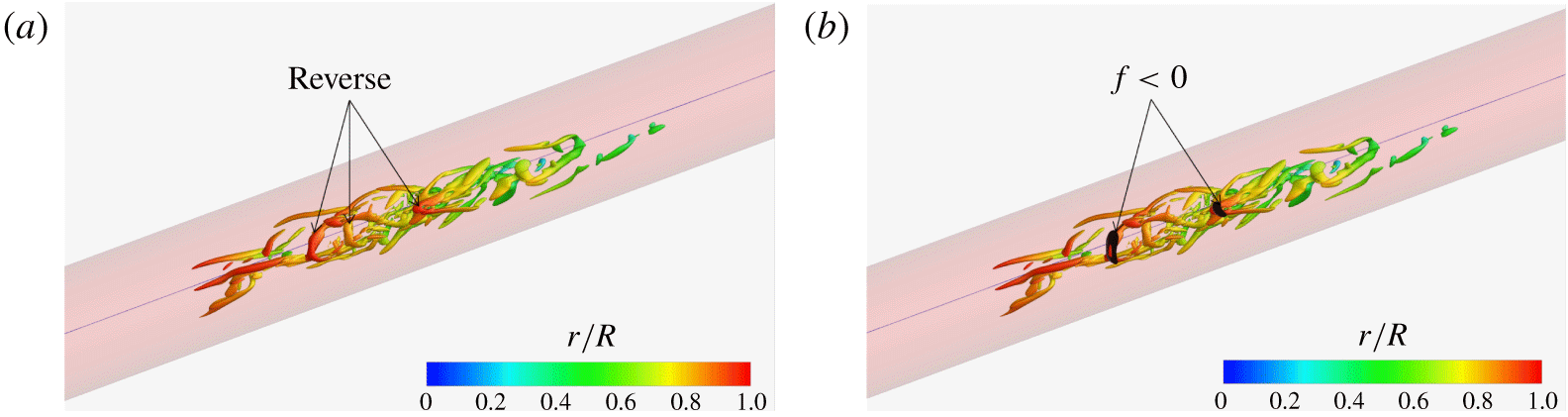
Figure 15(a) shows an infant turbulent spot from the present flow at  $t=213\,000\unicode[STIX]{x0394}t$, which is the same as that in figure 13(c) but without the high-speed streaks to better reveal the vortex structures. It is evident that this infant spot contains three reverse hairpins and two forward hairpin vortices. Note again that this spot is the predecessor of the more mature spot in figure 11 at
 $t=215\,000\unicode[STIX]{x0394}t$, and in figure 13(b) at
 $=214\,000\unicode[STIX]{x0394}t$. Figure 15(b) presents the isosurfaces of
 $\unicode[STIX]{x1D706}_{ci}=1.5$ (same as in figure 15(a), coloured based on
 $r/R$) and the isosurfaces of
 $u_{z}=-0.005V$ (coloured black). We have verified that the isosurfaces of such very weak negative axial velocity are located extremely close to the wall so that taking the derivative along the radial direction with respect to the zero velocity at the wall yields
 $f<0$. Thus, a patch of
 $u_{z}=-0.005V$ in the figure corresponds very well to a region of negative skin friction. It is evident that there are only two patches of
 $f<0$ in this region at
 $t=213\,000\unicode[STIX]{x0394}t$, and each of them is right beneath the head element of a reverse hairpin vortex. The middle reverse hairpin vortex is not associated with a negative skin-friction patch at this instant. Many other turbulent spot images similar to figure 15(b) are examined, and we found that, during transition, a negative skin-friction patch is almost always underneath the head element of a reverse hairpin vortex.
(a) Isosurfaces of  $\unicode[STIX]{x1D706}_{ci}=1.5V/R$ at
 $t=213\,000\unicode[STIX]{x0394}t$ showing the infant turbulent spot, which develops into the matured turbulent spot of figure 11. (b) Isosurface of
 $f<0$ (black) overlaid on the isosurfaces of
 $\unicode[STIX]{x1D706}_{ci}$ of (a). It is evident that during transition the negative skin-friction patch is found underneath the head element of a reverse hairpin vortex.

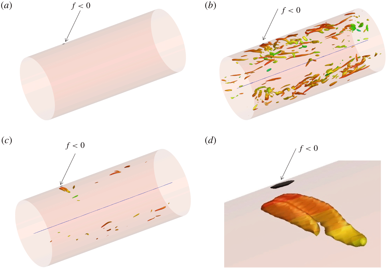
Figure 16(a) shows the negative skin-friction patch found at  $t=231\,000\unicode[STIX]{x0394}t$ in the range
 $422R<z<427R$ where the turbulent flow is fully developed. Only one patch of
 $f<0$ is seen in this zone, considerably fewer than in the transitional zone. In figure 16(b) the patch is overlaid with isosurfaces of
 $\unicode[STIX]{x1D706}_{ci}=3.0V/R$, and there is no obvious connection between the
 $f<0$ patch and the vortex structures. However, when weaker vortex structures are removed from the view with an increase of isosurface value to
 $\unicode[STIX]{x1D706}_{ci}=5.5V/R$ in figure 16(c), it becomes quite evident that the patch is right beneath a vortex structure. The zoomed view in figure 16(d) further demonstrates that the vortex structure above the
 $f<0$ patch is a reverse hairpin vortex. Corroborated with many other images like this, we found that in the fully developed turbulent pipe flow region, each negative skin-friction patch is also almost always underneath a reverse hairpin vortex.
(a) Isosurface of  $f<0$ (black) at
 $t=231\,000\unicode[STIX]{x0394}t$ in the fully developed turbulent region
 $422<z/R<427$; (b) isosurfaces of
 $\unicode[STIX]{x1D706}_{ci}=3.0V/R$ overlaid on the isosurface of
 $f<0$ (black); (c) isosurfaces of
 $\unicode[STIX]{x1D706}_{ci}=5.5V/R$ overlaid on the isosurface of
 $f<0$ (black); (d) magnified view of (c).

Thus, it is reasonable to arrive at an indirect estimate of the number density of reverse hairpin vortices in the present flow by counting the patches of negative skin friction, a procedure that avoids the challenges associated with auto-recognition or auto-untangling. We wrote a linked-list-based computer program to automatically identify, count and measure the size of each isolated patch with negative skin friction. The procedures are as follows. Step (i) is to extract the isosurfaces of streamwise velocity at a very small negative value ( $-5\times 10^{-3}V$) from a selected raw DNS volume file into a finite element three-dimensional surface data file. In this extraction process, the coordinates of the isosurfaces are exported into the finite element surface data file. Step (ii) is to check the connectivity of each element with all the other elements in the finite element file so that elements belonging to the same isolated patch are stored into one linked list. Step (iii) is to count the number of isolated patches, and to find the area and geometric centre of each patch from the finite element file corresponding to the originally selected raw DNS data volume. Steps (i) and (iii) are repeated for all the raw DNS files to be sampled to accumulate statistics.
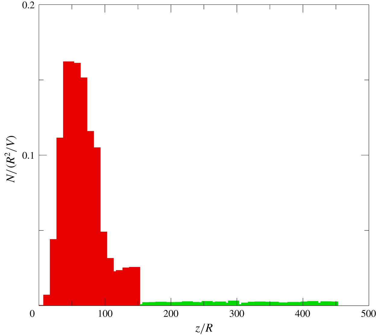
The number density of isolated  $f<0$ patches in the present flow is given in figure 17. Because we found that such patches almost always occur beneath the head element of a reverse hairpin vortex, the number density found in this way is an approximate estimate for the number density of the reverse hairpins in the flow. It is a conservative estimation because some reverse hairpins do not occur above an
 $f<0$ patch. Number density of isolated
 $f<0$ patches in Case S3R8 of Wu et al. (Reference Wu, Moin, Adrian and Baltzer2015) with a circumferential-mode inlet disturbance located at
 $0.4<r/R<0.42$ has also been computed, and it displays both qualitatively and quantitively similar characteristics to those in the present flow with a radial-mode inlet disturbance. Thus, the reverse hairpin generation paradigm in pipe turbulent spots is quite robust and valid under all the three types of inlet disturbance we considered: radial mode, circumferential mode close to the wall (Case S5R8) and circumferential mode in the pipe core region (Case S3R8 and Case S4R6). In figure 17, in order to increase the sample size, the statistics are bin averaged with a bin size of
 $10R$. It is seen that at the peak of transition, there are approximately 0.16 reverse hairpin vortices per unit axial length
 $R$ and per unit time
 $R/V$. The number density in the fully developed turbulent region shows small variation with axial distance, and the level is approximately 5 % of the value at the peak of transition.
Estimation of number density for reverse hairpin vortices in the present DNS, based on the number density of  $f<0$ patches per unit axial length
 $R$ and per unit time
 $R/V$. It is evident that the number density is substantially higher during transition (red) than in the fully developed turbulent region (green).

10 Concluding remarks
The experimental visualizations of Lindgren (Reference Lindgren1959a,Reference Lindgrenb,Reference Lindgrenc) revealed a puzzling feature: apparent ‘turbulent scalar patches’ residing in fully developed turbulent pipe flow several hundred radii downstream of transition. We performed a spatially developing pipe flow simulation from laminar through transition all the way to fully developed turbulent state in a 500 radius long pipe configuration at  $Re=6500$. Compared to the feasibility study of Wu et al. (Reference Wu, Moin, Adrian and Baltzer2015) using a localized circumferential-mode inlet perturbation, here, we adopted a radial-mode inlet disturbance through a narrow three degree numerical wedge within which the laminar velocity profile is replaced by a time-dependent turbulent field. Passive scalar is introduced into the computational domain at the inlet within the radial range of
 $0\leqslant r\leqslant 0.05$. Accuracy of the statistics is confirmed. Along the axial direction, the distribution of the passive scalar is segmented and propagates downstream with time. Scalar field segmentation originates from turbulent spots formed during pipe transition. Such scalar patches in the fully developed turbulent pipe flow carry a memory of transition events located far upstream. It is reasonable to argue that the ‘turbulent bentonite suspension patches’ observed by Lindgren in the fully turbulent pipe flow region are related to scalar field segmentation.
During the late stage of transition, second-order statistics such as Reynolds stresses and the rate of dissipation of turbulent kinetic energy overshoot substantially above their levels in the downstream fully developed turbulent flow. In order to account for the overshoot, frequency spectra for the rate of dissipation of turbulence kinetic energy were computed. It was found that spectra sampled in the late transitional region possess a stronger mid-to-high frequency content compared to those collected in the downstream fully developed turbulent region. Flow visualizations in the late transition region revealed bursts of small-scale vortex motions that probably account for the enhanced mid-to-high frequency spectral content. Both the wall-turbulence mechanism (i.e. the mechanism producing forward hairpin packets) and the inviscid Kelvin–Helmholtz instability mechanism are at play during the late stage of pipe transition. In combination, they contribute to the generation of more small-scale activity.
Mature transitional–turbulent spots are found to consist mostly of reverse hairpin vortices (in the near-wall region) with their head elements located upstream of the legs and close to the wall (‘feet first’), whereas the core region consists of forward hairpin vortices (‘head first’). The reverse hairpin vortices are due to high-speed streaks arising from the radial-mode inlet perturbation. High-speed streaks downstream of the inlet develop three-dimensional shear layers on their interface with the low-speed flow at the wall. The shear layers are unstable and subsequently break down and roll-up to form a concentrated succession of reverse hairpin vortices. The DNS data for Case S5R8 (Wu et al. Reference Wu, Moin, Adrian and Baltzer2015) under a circumferential-mode inlet perturbation were also examined, and the mature turbulent spots revealed essentially the same dual-type structural composition and the same high-speed streak effect in forming the reverse hairpins as in the current flow.
In both the transitional region and the fully developed turbulent flow region, a patch of negative skin friction almost always occurs beneath the head of a reverse hairpin vortex, although not every reverse hairpin vortex excites a negative skin-friction patch at each instant. This realization provided a means to indirectly count the number of reverse hairpin vortices through automatic enumeration of negative skin-friction patches, notwithstanding the under-countering. The acquired number density suggests that during the peak of transition there is approximately one reverse hairpin per unit axial length  $R$ for every
 $6R/V$ time units. In the fully developed turbulent region, the number density is only approximately 5 % of the peak level achieved during transition. Thus, in pipe flow the reverse hairpins are mostly a phenomenon of the transition region, and they die away to a very small number in the fully turbulent flow region.
Finally, it is interesting to note that the single initial goal of the present study was to clarify the origin of turbulent scalar patches in fully developed turbulent pipe flow. During the investigation, new questions arose about the flow physics underlying overshoot transition statistics, dual-type structural composition of turbulent spots and reverse hairpin enumeration. The answers to these new questions are perhaps at least as interesting as the answer to the original query.
Acknowledgements
R.J.A. would like to acknowledge the support of the US National Science Foundation and the Ira A. Fulton Endowment. P.M. is grateful for the support from the US Air Force Office of Scientific Research and Department of Energy. X.W. acknowledges the support from NSERC, Compute Canada and the 2016 Summer Research Program at the Center for Turbulence Research at Stanford University.
Declaration of interests
The authors report no conflict of interest.