1 Introduction
Starting with the pioneering works of Lamb (Reference Lamb1932), there is a long history of the development of analytic methods to investigate surface wavefield modifications induced by bathymetric changes. Interest in this problem is due to the phenomena associated with wave propagation over submarine trenches in the ocean or across navigational channels where changes in water depth are commonly the case. Recent years have seen renewed interest in this problem with the exciting idea to transpose the concept of metamaterials emerging from the physics community to water waves, see e.g. the introductory discussion in Porter (Reference Porter2017). Such metamaterial devices have been proposed to produce a lensing effect (Hu & Chan Reference Hu and Chan2005; Zhang, Chan & Hu Reference Zhang, Chan and Hu2014; Bobinski et al. Reference Bobinski, Eddi, Petitjeans, Maurel and Pagneux2015), to control the ocean wave energy flow (Chen et al. Reference Chen, Yang, Zi and Chan2009; Berraquero et al. Reference Berraquero, Maurel, Petitjeans and Pagneux2013; Dupont et al. Reference Dupont, Kimmoun, Molin, Guenneau and Enoch2015) or to produce a protected free wave region using cloaking strategies (Farhat et al. Reference Farhat, Enoch, Guenneau and Movchan2008; Newman Reference Newman2014; Porter & Newman Reference Porter and Newman2014; Xu et al. Reference Xu, Jiang, Fang, Georget, Abdeddaim, Geffrin, Farhat, Sabouroux, Enoch and Guenneau2015; Zareei & Alam Reference Zareei and Alam2015; Dupont et al. Reference Dupont, Guenneau, Kimmoun, Molin and Enoch2016; Porter Reference Porter2017). For most cases, the idea is to exploit an effective anisotropy resulting from a bathymetry varying at the subwavelength scale. A tempting approach to predicting this anisotropy relies on a two-step procedure, in which a three- to two-dimensional reduction (in the vertical direction) is firstly conducted, afterwards the homogenization of the resulting two-dimensional equation of the shallow water type is performed, thus benefitting from the analogy with the polarized Maxwell equations. In the case of a layer structured sea bed, this provides effective water depths that are simply the arithmetic and geometric averages of the actual ones, see e.g. Chen et al. (Reference Chen, Yang, Zi and Chan2009), Berraquero et al. (Reference Berraquero, Maurel, Petitjeans and Pagneux2013), Dupont et al. (Reference Dupont, Kimmoun, Molin, Guenneau and Enoch2015). As already stressed in Porter & Newman (Reference Porter and Newman2014) and in Porter (Reference Porter2017), the validity of the shallow water equations is restricted to bed gradients that are small compared to the typical wavelength, which is rarely fulfilled. Besides, it has been shown in Rosales & Papanicolaou (Reference Rosales and Papanicolaou1983) that conducting the homogenization of the full three-dimensional problem results in effective water depths depending on the resolution of cell problems which interrogate effects of the evanescent field, or transition effects, in the water channel, see also Mei et al. (Reference Mei, Chan, Liu, Huang and Zhang2011), Wang, Guo & Mei (Reference Wang, Guo and Mei2015), Guo et al. (Reference Guo, Wang, Mei and Liu2017). Recently, this result has been validated experimentally (Maurel et al. Reference Maurel, Marigo, Cobelli, Petitjeans and Pagneux2017); for a simple layered microstructures, it has been shown that it is possible to play with the three-dimensional effects to get an anisotropy significantly higher than that predicted by the homogenized two-dimensional shallow water wave equation.
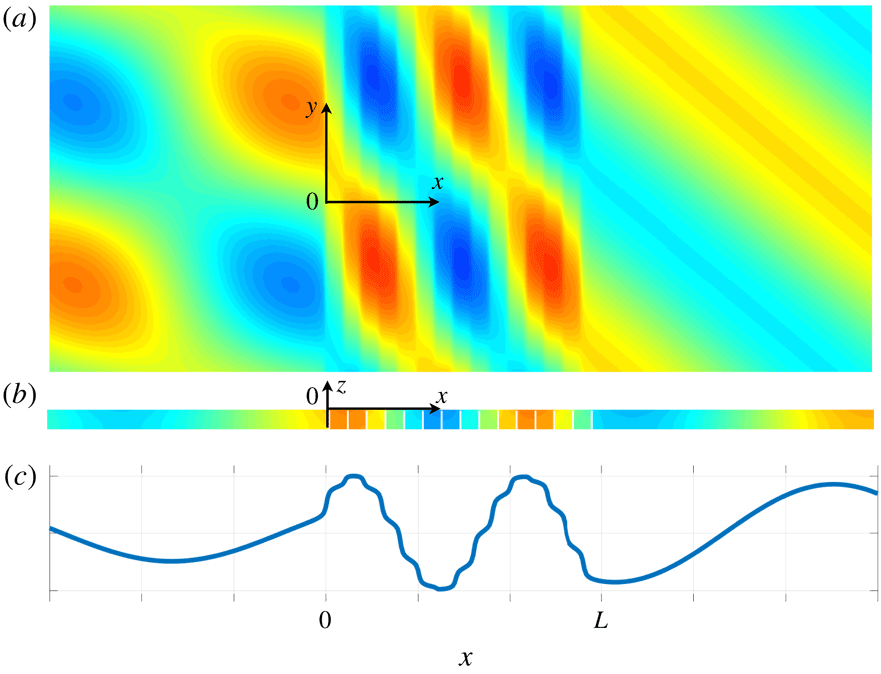
Scattering by a structured ridge of finite extent (computed numerically). The region
 $(0,L)$
contains
 $N=15$
layers alternating
 $h^{-}=0.05$
of relative thickness
 $\unicode[STIX]{x1D709}=0.1$
and
 $h^{+}=1$
(the spacing is
 $\ell =1$
); outside the ridge,
 $h=1$
. The incident wave comes from the left at incidence
 $\unicode[STIX]{x1D703}=50^{\circ }$
and frequency
 $\unicode[STIX]{x1D714}\sqrt{h/g}=0.4$
. (a) The free surface elevation (
 $\unicode[STIX]{x1D711}_{\mathit{num}}(x,y,0)$
), (b) field of the potential in a vertical section
 $\unicode[STIX]{x1D711}_{\mathit{num}}(x,0,z)$
and (c) profile of the free surface elevation
 $\unicode[STIX]{x1D711}_{\mathit{num}}(x,0,0)$
.

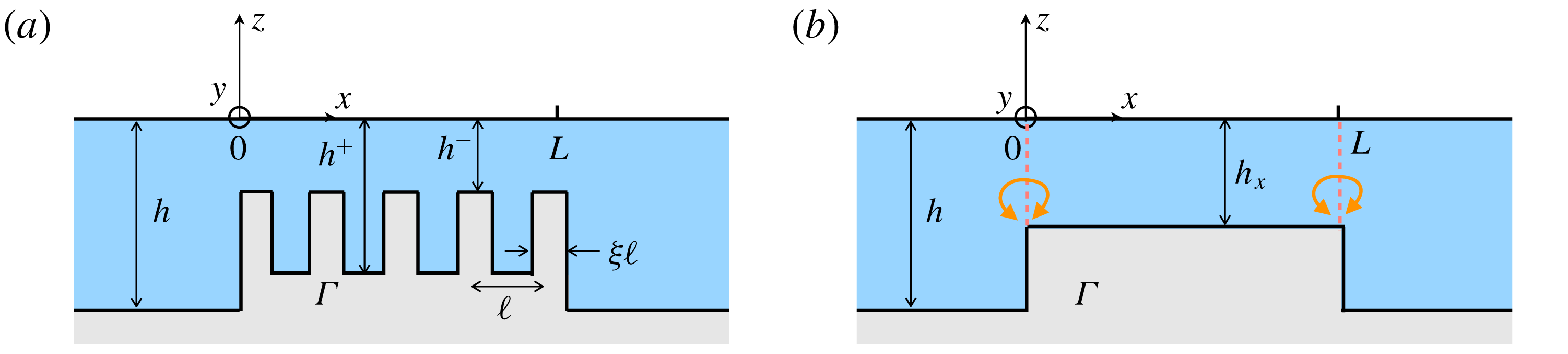
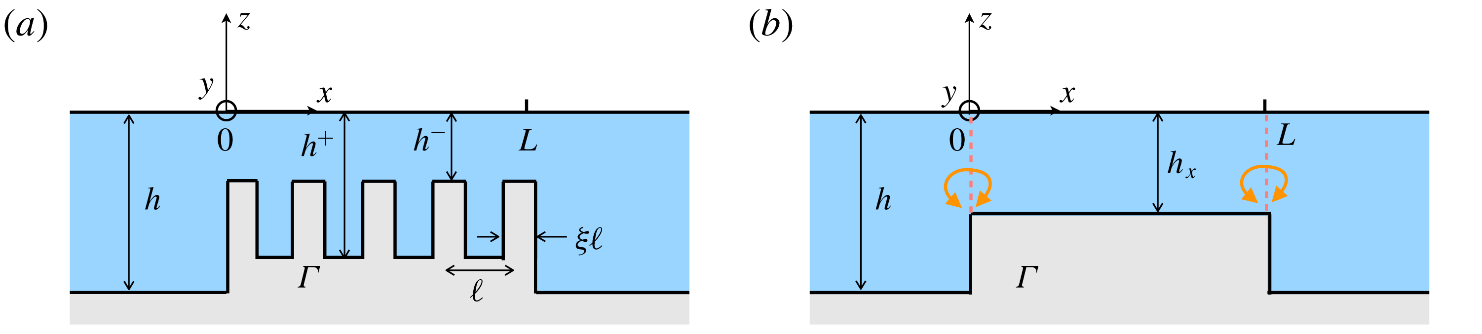
In the present study, we extend the homogenization procedure and address the problem of scattering by a structured ridge of finite extent, see figure 1. Specifically, we focus on the transmission conditions which complement the homogenized two-dimensional equation, and which encapsulate the effects of the evanescent field at the end boundaries of the ridge, as shown in figure 2. We shall establish that at the dominant, first, order these conditions are the intuitive continuities of the surface elevation and of the normal mass flux while at second order these two fields are discontinuous. The derivation of such unusual transmission conditions are classical for piecewise constant water channels using matched asymptotic techniques (Tuck Reference Tuck1976) and we shall see that our result includes this limiting case. In the present case, matched asymptotic techniques have to be combined with homogenization and there are only few works dealing with such methods, see e.g. Cakoni, Guzina & Moskow (Reference Cakoni, Guzina and Moskow2016), Vinoles (Reference Vinoles2016), Marigo & Maurel (Reference Marigo and Maurel2017) and Maurel & Marigo (Reference Maurel and Marigo2018). It is worth noting that these unusual transmission conditions are corrections to the intuitive ones and as such we could expect that they have a weak influence on the scattering properties. In fact, we shall illustrate that their influence can be very significant since the leading-order model may fail dramatically even at relatively low frequencies. Such failure has already been reported in Sheinfux et al. (Reference Sheinfux, Kaminer, Plotnik, Bartal and Segev2014) for the scattering of electromagnetic waves by stratified structures, and analysed in Maurel & Marigo (Reference Maurel and Marigo2018) using a similar approach. We also mention a recent work by Porter (Reference Porter2019) which demonstrates the significant improvement due to second-order corrections in an extended version of the shallow water equation; in this case, a discontinuity in the gradient of the sea bed gives rise to a discontinuous surface elevation.
The outline of the rest of the paper is as follows. In § 2, we give the statement of the scattering problem by a structured ridge surrounded by regions of constant depth and we present the homogenized model up to the second order. The derivation of this model is detailed in §§ 3 and 4. In § 3, the homogenization is performed far from the end boundaries of the ridge. Although this procedure simply follows that conducted by Rosales & Papanicolaou (Reference Rosales and Papanicolaou1983), it allows us to define the fields at the two first orders and to introduce auxiliary problems, often termed cell problems, which are needed to set the problem at the end boundary of the structure. This problem and the resulting transmission conditions are presented in § 4. The properties of the homogenized models are discussed in § 5 and their validity is inspected in § 6 by comparison with the complete solution computed numerically. In particular, the sensitivity of the scattering properties to the geometry of the layers terminating the ridge is exemplified.


2 The actual and the effective problems
Using the assumptions of an inviscid, incompressible fluid, and an irrotational motion, the velocity potential
 $\unicode[STIX]{x1D711}^{\mathit{3d}}(\boldsymbol{r},z)$
and the associated velocity
 $\boldsymbol{u}^{\mathit{3d}}(\boldsymbol{r},z)$
satisfy in the transient regime the full three-dimensional problem
 $$\begin{eqnarray}\displaystyle \left.\begin{array}{@{}l@{}}\displaystyle \boldsymbol{u}^{\mathit{3d}}=\unicode[STIX]{x1D735}\unicode[STIX]{x1D711}^{\mathit{3d}}+\frac{\unicode[STIX]{x2202}\unicode[STIX]{x1D711}^{\mathit{3d}}}{\unicode[STIX]{x2202}z}\,\boldsymbol{e}_{\mathit{z}},\quad \text{div}\,\boldsymbol{u}^{\mathit{3d}}+\frac{\unicode[STIX]{x2202}u_{z}^{\mathit{3d}}}{\unicode[STIX]{x2202}z}=0,\\[10.0pt] \displaystyle {u_{z}^{\mathit{3d}}}_{|z=0}=-\frac{1}{g}\,{\unicode[STIX]{x2202}_{tt}\unicode[STIX]{x1D711}^{\mathit{3d}}}_{|z=0},\quad \boldsymbol{u}^{\mathit{3d}}\boldsymbol{\cdot }\boldsymbol{n}_{|\unicode[STIX]{x1D6E4}}=0,\end{array}\right\} & & \displaystyle\end{eqnarray}$$
with
 $g$
the gravitational constant;
 $t$
is the time,
 $\boldsymbol{r}=(x,y)$
is the coordinate in the horizontal plane (
 $\unicode[STIX]{x1D735}$
and
 $\text{div}$
are the gradient and the divergence with respect to
 $\boldsymbol{r}$
),
 $z$
is the vertical coordinate. Next,
 $z=0$
is the undisturbed free surface and
 $\unicode[STIX]{x1D6E4}$
denotes the boundary of the sea bottom (
 $\unicode[STIX]{x2202}_{n}\unicode[STIX]{x1D711}^{\mathit{3d}}$
is the normal derivative of
 $\unicode[STIX]{x1D711}^{\mathit{3d}}$
).
In the time domain, the shallow water regime is guaranteed if the maximum frequency
 $\unicode[STIX]{x1D714}$
imposed by the source satisfies
 $\unicode[STIX]{x1D714}^{2}h/g\ll 1$
with
 $h$
the typical immersion depth and we restrict our study to this case. We consider also that the array spacing
 $\ell$
is of the same order of magnitude as
 $h$
. Following Rosales & Papanicolaou (Reference Rosales and Papanicolaou1983), we shall establish that the effective homogenized problem is reduced to a two-dimensional problem for a two-dimensional potential
 $\unicode[STIX]{x1D711}(\boldsymbol{r})$
and it reads
 $$\begin{eqnarray}\displaystyle \left.\begin{array}{@{}ll@{}}\displaystyle h\,\unicode[STIX]{x1D6FB}^{2}\unicode[STIX]{x1D711}(\boldsymbol{r})-\frac{1}{g}\,\unicode[STIX]{x2202}_{tt}\unicode[STIX]{x1D711}(\boldsymbol{r})=0, & \text{over channels of constant depth }h,\\[10.0pt] \displaystyle h_{x}\,\frac{\unicode[STIX]{x2202}^{2}\unicode[STIX]{x1D711}}{\unicode[STIX]{x2202}x^{2}}(\boldsymbol{r})+h_{y}\,\frac{\unicode[STIX]{x2202}^{2}\unicode[STIX]{x1D711}}{\unicode[STIX]{x2202}y^{2}}(\boldsymbol{r})-\frac{1}{g}\,\unicode[STIX]{x2202}_{tt}\unicode[STIX]{x1D711}(\boldsymbol{r})=0, & \text{over a structured ridge}.\end{array}\right\}\quad & & \displaystyle\end{eqnarray}$$
In the case of the microstructure varying along
 $x$
only, with a periodicity
 $\ell$
, we get
 $$\begin{eqnarray}\displaystyle h_{x}=\ell \,\int _{\unicode[STIX]{x1D6FA}}\left(\frac{\unicode[STIX]{x2202}\unicode[STIX]{x1D6F7}}{\unicode[STIX]{x2202}x_{\mathit{r}}}+1\right)\,\text{d}x_{r}\,\text{d}z_{\mathit{r}},\quad h_{y}=\langle h\rangle , & & \displaystyle\end{eqnarray}$$
where
 $\unicode[STIX]{x1D6F7}(x_{\mathit{r}},z_{\mathit{r}})$
is the solution of a static problem, see forthcoming equation (3.18), set in coordinates
 $(x_{\mathit{r}},z_{\mathit{r}})$
rescaled with the spacing
 $\ell$
, where
 $\unicode[STIX]{x1D6FA}$
is the unit cell containing a single microstructure; also,
 $\langle .\rangle$
means the average over
 $\unicode[STIX]{x1D6FA}$
. Hence, only
 $h_{x}$
is impacted by the transition effects in the water depth. Now, defining the normal flux
 $D(\boldsymbol{r})$
as
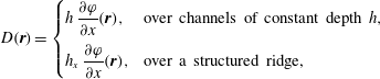 $$\begin{eqnarray}\displaystyle D(\boldsymbol{r})=\left\{\begin{array}{@{}ll@{}}\displaystyle h\,\frac{\unicode[STIX]{x2202}\unicode[STIX]{x1D711}}{\unicode[STIX]{x2202}x}(\boldsymbol{r}), & \text{over channels of constant depth }h,\\[10.0pt] \displaystyle h_{x}\,\frac{\unicode[STIX]{x2202}\unicode[STIX]{x1D711}}{\unicode[STIX]{x2202}x}(\boldsymbol{r}), & \text{over a structured ridge,}\end{array}\right. & & \displaystyle\end{eqnarray}$$
non-intuitive transmission conditions apply at the boundary between the two regions, say at
 $x=0$
, of the form
 $$\begin{eqnarray}\displaystyle \displaystyle \unicode[STIX]{x27E6}\unicode[STIX]{x1D711}\unicode[STIX]{x27E7}={\mathcal{B}}\,\overline{D},\quad \displaystyle \unicode[STIX]{x27E6}D\unicode[STIX]{x27E7}=\ell ^{2}{\mathcal{C}}\,\frac{\unicode[STIX]{x2202}^{2}\overline{\unicode[STIX]{x1D711}}}{\unicode[STIX]{x2202}y^{2}}, & & \displaystyle\end{eqnarray}$$
where we defined the jump
 $\unicode[STIX]{x27E6}\unicode[STIX]{x1D711}\unicode[STIX]{x27E7}=\unicode[STIX]{x1D711}(0^{+},y)-\unicode[STIX]{x1D711}(0^{-},y)$
and the mean value
 $\overline{\unicode[STIX]{x1D711}}=(1/2)(\unicode[STIX]{x1D711}(0^{+},y)+\unicode[STIX]{x1D711}(0^{-},y))$
(the same for
 $D$
). It is worth noting that the effective problem, equations (2.2)–(2.5), is simpler than the actual one in (2.1) because the region containing the microstructure at the small scale
 $\ell$
has been replaced by a region (of same extent) made of an anisotropic but homogeneous medium. This is the basic simplification expected from the homogenization process. Next, a dimensional reduction from a three-dimensional problem to a two-dimensional problem has been obtained owing to the shallow water hypothesis. We shall now detail the derivation of this model using a combination of the techniques of two scale homogenization and of matched asymptotic expansions.
3 Propagation in regions with constant depth and structured sea bed
The asymptotic analysis is performed owing to the two typical length scales separated by
 $\unicode[STIX]{x1D700}$
. The small scales are
 $\ell$
, the spacing of the microstructure, and the water depth
 $h$
is of the same order of magnitude. In the transient regime, we assume that the source imposes a maximum frequency
 $\unicode[STIX]{x1D714}$
, hence a smallest wavelength
 $\sqrt{g\ell }/\unicode[STIX]{x1D714}$
, and we set
 $$\begin{eqnarray}\displaystyle \unicode[STIX]{x1D700}=\unicode[STIX]{x1D714}\sqrt{\frac{\ell }{g}}\ll 1\quad \text{and}\quad \unicode[STIX]{x1D714}\sqrt{\frac{h}{g}}=O(\unicode[STIX]{x1D700}). & & \displaystyle\end{eqnarray}$$
In this section, we write the problem in non-dimensional form, with
 $$\begin{eqnarray}\displaystyle t\rightarrow \unicode[STIX]{x1D714}t,\quad \boldsymbol{r}\rightarrow \frac{\unicode[STIX]{x1D714}\boldsymbol{r}}{\sqrt{g\ell }},\quad z\rightarrow \frac{\unicode[STIX]{x1D714}z}{\sqrt{g\ell }},\quad \boldsymbol{u}^{\mathit{3d}}\rightarrow \frac{\boldsymbol{u}^{\mathit{3d}}}{u_{0}},\quad \unicode[STIX]{x1D711}^{\mathit{3d}}\rightarrow \frac{\unicode[STIX]{x1D714}}{\sqrt{g\ell }}\frac{\unicode[STIX]{x1D711}^{\mathit{3d}}}{u_{0}}, & & \displaystyle\end{eqnarray}$$
from which (2.1) reads as
 $$\begin{eqnarray}\displaystyle \left.\begin{array}{@{}l@{}}\displaystyle \boldsymbol{u}^{\mathit{3d}}=\unicode[STIX]{x1D735}\unicode[STIX]{x1D711}^{\mathit{3d}}+\unicode[STIX]{x2202}_{z}\unicode[STIX]{x1D711}^{\mathit{3d}},\quad \text{div}\,\boldsymbol{u}^{\mathit{3d}}+\unicode[STIX]{x2202}_{z}u_{z}^{\mathit{3d}}=0,\\ \displaystyle {u_{z}^{\mathit{3d}}}_{|z=0}=-\unicode[STIX]{x1D700}\,\unicode[STIX]{x2202}_{tt}\unicode[STIX]{x1D711}^{\mathit{3d}}_{|z=0},\quad \boldsymbol{u}^{\mathit{3d}}\boldsymbol{\cdot }\boldsymbol{n}_{|\unicode[STIX]{x1D6E4}}=0.\end{array}\right\} & & \displaystyle\end{eqnarray}$$
Next, the separation of scales is accounted for using two coordinate systems, with
 $$\begin{eqnarray}\displaystyle \boldsymbol{r}=(x,y),\quad \text{and}\quad (x_{\mathit{r}},z_{\mathit{r}})=\left(\frac{x}{\unicode[STIX]{x1D700}},\frac{z}{\unicode[STIX]{x1D700}}\right). & & \displaystyle\end{eqnarray}$$
The macroscopic coordinate
 $\boldsymbol{r}$
is adopted to describe the slow variations of the surface waves propagating at the free surface, while the microscopic coordinate
 $(x_{\mathit{r}},z_{\mathit{r}})$
is adopted to describe the rapid variations of the evanescent field along
 $x_{\mathit{r}}$
due to the microstructure and in the vertical direction because of the shallow regime.
3.1 A warm up and useful result – propagation in a region of constant depth
To begin with, we shall recover the shallow water equation over channels of constant depth
 $h$
. To do so, we consider the following expansions
 $$\begin{eqnarray}\displaystyle \displaystyle \unicode[STIX]{x1D711}^{\mathit{3d}}=\unicode[STIX]{x1D711}^{0}(\boldsymbol{r},z_{\mathit{r}})+\unicode[STIX]{x1D700}\unicode[STIX]{x1D711}^{1}(\boldsymbol{r},z_{\mathit{r}})+\cdots \,,\quad \boldsymbol{u}^{\mathit{3d}}=\boldsymbol{u}^{0}(\boldsymbol{r},z_{\mathit{r}})+\unicode[STIX]{x1D700}\boldsymbol{u}^{1}(\boldsymbol{r},z_{\mathit{r}})+\cdots \,, & & \displaystyle\end{eqnarray}$$
and the horizontal gradient is replaced by
 $$\begin{eqnarray}\displaystyle \unicode[STIX]{x1D735}+\frac{\boldsymbol{e}_{\mathit{z}}}{\unicode[STIX]{x1D700}}\frac{\unicode[STIX]{x2202}}{\unicode[STIX]{x2202}z_{\mathit{r}}},\quad \text{with }\unicode[STIX]{x1D735}=\boldsymbol{e}_{\mathit{x}}\,\frac{\unicode[STIX]{x2202}}{\unicode[STIX]{x2202}x}+\boldsymbol{e}_{\mathit{y}}\,\frac{\unicode[STIX]{x2202}}{\unicode[STIX]{x2202}y}, & & \displaystyle\end{eqnarray}$$
so that (3.3) becomes, for
 $n\geqslant 0$
,
 $$\begin{eqnarray}\displaystyle \left.\begin{array}{@{}l@{}}\displaystyle \frac{\unicode[STIX]{x2202}\unicode[STIX]{x1D711}^{0}}{\unicode[STIX]{x2202}z_{\mathit{r}}}=0,\quad \boldsymbol{u}^{n}=\unicode[STIX]{x1D735}\unicode[STIX]{x1D711}^{n}+\frac{\unicode[STIX]{x2202}\unicode[STIX]{x1D711}^{n+1}}{\unicode[STIX]{x2202}z_{\mathit{r}}}\,\boldsymbol{e}_{\mathit{z}},\\[12.0pt] \displaystyle \frac{\unicode[STIX]{x2202}u_{z}^{0}}{\unicode[STIX]{x2202}z_{\mathit{r}}}=0,\quad \text{div}\,\boldsymbol{u}^{n}+\frac{\unicode[STIX]{x2202}u_{z}^{n+1}}{\unicode[STIX]{x2202}z_{\mathit{r}}}=0,\\[12.0pt] \displaystyle {u_{z}^{0}}_{|z_{\mathit{r}}=0}=0,\quad {u_{z}^{n+1}}_{|z_{\mathit{r}}=0}=-\unicode[STIX]{x2202}_{tt}{\unicode[STIX]{x1D711}^{n}}_{|z_{\mathit{r}}=0},\quad {u_{z}^{n}}_{|z_{\mathit{r}}=-h^{\ast }}=0,\end{array}\right\} & & \displaystyle\end{eqnarray}$$
where
 $h^{\ast }=h/\ell$
is the channel depth in dimensionless form.
3.2 The first order
From (3.7),
 $\unicode[STIX]{x1D711}^{0}$
and
 $u_{z}^{0}$
do not depend on
 $z_{\mathit{r}}$
. Besides, since
 $u_{z}^{0}(\boldsymbol{r})$
vanishes at
 $z_{\mathit{r}}=0$
, we deduce that
 $u_{z}^{0}=0$
and eventually
 $$\begin{eqnarray}\displaystyle \boldsymbol{u}^{0}(\boldsymbol{r})=\unicode[STIX]{x1D735}\unicode[STIX]{x1D711}^{0}(\boldsymbol{r}). & & \displaystyle\end{eqnarray}$$
Also, it follows from
 $0=u_{z}^{0}=\unicode[STIX]{x2202}_{z_{\mathit{r}}}\unicode[STIX]{x1D711}^{1}$
that
 $\unicode[STIX]{x1D711}^{1}(\boldsymbol{r})$
does not depend on
 $z_{\mathit{r}}$
, hence
 $$\begin{eqnarray}\displaystyle \boldsymbol{u}^{1}(\boldsymbol{r},z_{\mathit{r}})=\unicode[STIX]{x1D735}\unicode[STIX]{x1D711}^{1}(\boldsymbol{r})+\frac{\unicode[STIX]{x2202}u_{z}^{2}}{\unicode[STIX]{x2202}z_{\mathit{r}}}(\boldsymbol{r},z_{\mathit{r}})\;\boldsymbol{e}_{z}, & & \displaystyle\end{eqnarray}$$
and
 $\text{div}\,\boldsymbol{u}^{1}=\unicode[STIX]{x1D6FB}^{2}\unicode[STIX]{x1D711}^{1}(\boldsymbol{r})$
since the divergence is two-dimensional. Thus, integrating for
 $n=0,1$
the relation
 $\text{div}\,\boldsymbol{u}^{n}+\unicode[STIX]{x2202}_{z_{\mathit{r}}}u_{z}^{n+1}=0$
between
 $z_{\mathit{r}}=-h^{\ast }$
and
 $z_{\mathit{r}}=0$
, along with the boundary conditions
 ${u_{z}^{n+1}}_{|z_{\mathit{r}}=-h^{\ast }}=0$
and
 ${u_{z}^{n+1}}_{|z_{\mathit{r}}=0}=\unicode[STIX]{x2202}_{tt}\unicode[STIX]{x1D711}^{n}(\boldsymbol{r})$
, we get that
 $$\begin{eqnarray}\displaystyle \left.\begin{array}{@{}l@{}}\displaystyle h^{\ast }\unicode[STIX]{x1D6FB}^{2}\unicode[STIX]{x1D711}^{0}(\boldsymbol{r})-\unicode[STIX]{x2202}_{tt}\unicode[STIX]{x1D711}^{0}(\boldsymbol{r})=0,\\[4.0pt] \displaystyle h^{\ast }\unicode[STIX]{x1D6FB}^{2}\unicode[STIX]{x1D711}^{1}(\boldsymbol{r})-\unicode[STIX]{x2202}_{tt}\unicode[STIX]{x1D711}^{1}(\boldsymbol{r})=0,\end{array}\right\} & & \displaystyle\end{eqnarray}$$
which is the usual shallow water equation applying at the first and second orders.
3.3 Effective propagation in a region with structured sea bed
Over the structured ridge and far away from its end boundaries, we assume that the fields can be expanded as follows
 $$\begin{eqnarray}\displaystyle \unicode[STIX]{x1D711}^{\mathit{3d}}=\unicode[STIX]{x1D711}^{0}(\boldsymbol{r},x_{\mathit{r}},z_{\mathit{r}})+\unicode[STIX]{x1D700}\unicode[STIX]{x1D711}^{1}(\boldsymbol{r},x_{\mathit{r}},z_{\mathit{r}})+\cdots \,,\quad \boldsymbol{u}^{\mathit{3d}}=\boldsymbol{u}^{0}(\boldsymbol{r},x_{\mathit{r}},z_{\mathit{r}})+\unicode[STIX]{x1D700}\boldsymbol{u}^{1}(\boldsymbol{r},x_{\mathit{r}},z_{\mathit{r}})+\cdots \,, & & \displaystyle \nonumber\\ \displaystyle & & \displaystyle\end{eqnarray}$$
with
 $\boldsymbol{r}=(x,y)$
well suited to describe the variations of the propagating field at the wavelength scale, and
 $(x_{\mathit{r}},z_{\mathit{r}})$
well suited to describe the variations of the evanescent field in the vertical direction (as previously) and along
 $x$
because of the microstructure. In this region, the horizontal gradient is replaced by
 $$\begin{eqnarray}\displaystyle \unicode[STIX]{x1D735}+\frac{1}{\unicode[STIX]{x1D700}}\,\unicode[STIX]{x1D735}_{\mathit{r}},\quad \text{with }\unicode[STIX]{x1D735}_{\mathit{r}}=\boldsymbol{e}_{\mathit{x}}\,\frac{\unicode[STIX]{x2202}}{\unicode[STIX]{x2202}x_{\mathit{r}}}+\boldsymbol{e}_{\mathit{z}}\,\frac{\unicode[STIX]{x2202}}{\unicode[STIX]{x2202}z_{\mathit{r}}}, & & \displaystyle\end{eqnarray}$$
and
 $\unicode[STIX]{x1D735}$
is defined in (3.6); it is useful to remark that
 $$\begin{eqnarray}\displaystyle \text{div}\,\unicode[STIX]{x1D735}_{\mathit{r}}=\text{div}_{\mathit{r}}\unicode[STIX]{x1D735}=\frac{\unicode[STIX]{x2202}^{2}}{\unicode[STIX]{x2202}x\unicode[STIX]{x2202}x_{\mathit{r}}}. & & \displaystyle\end{eqnarray}$$
In addition, we assume that
 $\unicode[STIX]{x1D711}^{n}$
and
 $\boldsymbol{u}^{n}$
are periodic with respect to
 $x_{\mathit{r}}$
, and we define
 $\unicode[STIX]{x1D6FA}$
the elementary cell in
 $(x_{\mathit{r}},z_{\mathit{r}})$
coordinates, with
 $x_{\mathit{r}}\in (-1/2,1/2)$
(figure 3). Now, equation (2.1) reads as
 $$\begin{eqnarray}\displaystyle \left.\begin{array}{@{}l@{}}\displaystyle \unicode[STIX]{x1D735}_{\mathit{r}}\unicode[STIX]{x1D711}^{0}=0,\quad \boldsymbol{u}^{n}=\unicode[STIX]{x1D735}_{\mathit{r}}\unicode[STIX]{x1D711}^{n+1}+\unicode[STIX]{x1D735}\unicode[STIX]{x1D711}^{n},\\[4.0pt] \displaystyle \text{div}_{\mathit{r}}\,\boldsymbol{u}^{0}=0,\quad \text{div}_{\mathit{r}}\,\boldsymbol{u}^{n+1}+\text{div}\,\boldsymbol{u}^{n}=0,\\[4.0pt] \displaystyle {u_{z}^{0}}_{|z_{\mathit{r}}=0}=0,\quad {u_{z}^{n+1}}_{|z_{\mathit{r}}=0}=-\unicode[STIX]{x2202}_{tt}{\unicode[STIX]{x1D711}^{n}}_{|z_{\mathit{r}}=0},\quad \boldsymbol{u}^{n}\boldsymbol{\cdot }\boldsymbol{n}_{|\unicode[STIX]{x1D6E4}}=0,\\[4.0pt] \unicode[STIX]{x1D711}^{n},\boldsymbol{u}^{n}\;\text{periodic with respect to}~x_{\mathit{r}}.\end{array}\right\} & & \displaystyle\end{eqnarray}$$
Homogenization in the bulk. On the left, the ridge of finite extent in
 $(x,y,z)$
coordinates (
 $\boldsymbol{r}=(x,y)$
). On the right, the unit cell
 $\unicode[STIX]{x1D6FA}$
in rescaled in
 $(x_{\mathit{r}},z_{\mathit{r}})$
coordinates, with
 $h^{\ast }(x_{\mathit{r}})=h(x/\unicode[STIX]{x1D700})/\ell$
.

3.3.1 First order
At the leading order in
 $1/\unicode[STIX]{x1D700}$
, equation (3.14) gives
 $\unicode[STIX]{x1D735}_{\mathit{r}}\unicode[STIX]{x1D711}^{0}=0$
, from which
 $\unicode[STIX]{x1D711}^{0}(\boldsymbol{r})$
depends on the macroscopic coordinates
 $\boldsymbol{r}$
only. It follows that
 $\unicode[STIX]{x1D711}^{1}(\boldsymbol{r},x_{\mathit{r}},z_{\mathit{r}})$
satisfies the following problem
 $$\begin{eqnarray}\displaystyle \left.\begin{array}{@{}l@{}}\displaystyle \unicode[STIX]{x1D6FB}_{\mathit{r}}^{2}\unicode[STIX]{x1D711}^{1}=0,\\[4.0pt] \displaystyle \frac{\unicode[STIX]{x2202}\unicode[STIX]{x1D711}^{1}}{\unicode[STIX]{x2202}z_{\mathit{r}}}_{|z_{\mathit{r}}=0}=0,\quad \unicode[STIX]{x1D735}_{\mathit{r}}\unicode[STIX]{x1D711}^{1}\boldsymbol{\cdot }\boldsymbol{n}=-\frac{\unicode[STIX]{x2202}\unicode[STIX]{x1D711}^{0}}{\unicode[STIX]{x2202}x}(\boldsymbol{r})\,{n_{x}}_{|\unicode[STIX]{x1D6E4}},\\[10.0pt] \unicode[STIX]{x1D711}^{1},\quad \unicode[STIX]{x1D735}_{\mathit{r}}\unicode[STIX]{x1D711}^{1}\text{ periodic with respect to}~x_{\mathit{r}},\end{array}\right\} & & \displaystyle\end{eqnarray}$$
where we have used that
 $\unicode[STIX]{x1D735}\unicode[STIX]{x1D711}^{0}\boldsymbol{\cdot }\boldsymbol{n}=\unicode[STIX]{x2202}_{x}\unicode[STIX]{x1D711}^{0}\,n_{x}$
(since the problem is invariant along
 $y$
hence
 $n_{y}=0$
). Next, the velocity at the leading order reads as
 $$\begin{eqnarray}\displaystyle \boldsymbol{u}^{0}(\boldsymbol{r},x_{\mathit{r}},z_{\mathit{r}})=\unicode[STIX]{x1D735}\unicode[STIX]{x1D711}^{0}(\boldsymbol{r})+\unicode[STIX]{x1D735}_{\mathit{r}}\unicode[STIX]{x1D711}^{1}(\boldsymbol{r},x_{\mathit{r}},z_{\mathit{r}}). & & \displaystyle\end{eqnarray}$$
The problem (3.15) is linear with respect to
 $\unicode[STIX]{x2202}_{x}\unicode[STIX]{x1D711}^{0}(\boldsymbol{r})$
so that we can set
 $$\begin{eqnarray}\displaystyle \unicode[STIX]{x1D711}^{1}(\boldsymbol{r},x_{\mathit{r}},z_{\mathit{r}})=\frac{\unicode[STIX]{x2202}\unicode[STIX]{x1D711}^{0}}{\unicode[STIX]{x2202}x}(\boldsymbol{r})\,\unicode[STIX]{x1D6F7}(x_{\mathit{r}},z_{\mathit{r}})+\langle \unicode[STIX]{x1D711}^{1}\rangle (\boldsymbol{r}), & & \displaystyle\end{eqnarray}$$
with
 $\unicode[STIX]{x1D6F7}$
satisfying the two-dimensional cell problem defined in
 $\unicode[STIX]{x1D6FA}$
 $$\begin{eqnarray}\displaystyle \left.\begin{array}{@{}l@{}}\unicode[STIX]{x1D6FB}_{\mathit{r}}^{2}\unicode[STIX]{x1D6F7}=0,\quad \text{in}\;\unicode[STIX]{x1D6FA}\\[4.0pt] \displaystyle \frac{\unicode[STIX]{x2202}\unicode[STIX]{x1D6F7}}{\unicode[STIX]{x2202}z_{\mathit{r}}}(x_{\mathit{r}},0)=0,\quad \displaystyle \frac{\unicode[STIX]{x2202}\unicode[STIX]{x1D6F7}}{\unicode[STIX]{x2202}n}_{|\unicode[STIX]{x1D6E4}}=-n_{x},\quad \unicode[STIX]{x1D6F7},\quad \unicode[STIX]{x2202}_{x_{\mathit{r}}}\unicode[STIX]{x1D6F7}\;\text{periodic with respect to}~x_{\mathit{r}}.\end{array}\right\}\quad & & \displaystyle\end{eqnarray}$$
Example of field
 $\unicode[STIX]{x1D6F7}(x_{\mathit{r}},z_{\mathit{r}})$
solution of (3.18) in the unit cell
 $\unicode[STIX]{x1D6FA}$
(
 $h^{+}/\ell =1$
,
 $h^{-}/\ell =0.3$
and
 $\unicode[STIX]{x1D709}=0.4$
).

It is worth noting that this problem is independent of the frequency, and
 $(\unicode[STIX]{x1D6F7}+x_{\mathit{r}})$
corresponds to the problem of potential flow in a corrugated rigid duct (figure 4). In (3.15),
 $\unicode[STIX]{x1D711}^{1}$
is defined up to a function of
 $\boldsymbol{r}$
; in (3.17), we have fixed this function equal to
 $$\begin{eqnarray}\displaystyle \langle \unicode[STIX]{x1D711}^{1}\rangle (\boldsymbol{r})=\frac{1}{\langle h^{\ast }\rangle }\int _{\unicode[STIX]{x1D6FA}}\unicode[STIX]{x1D711}^{1}(\boldsymbol{r},x_{\mathit{r}},z_{\mathit{r}})\,\text{d}x_{r}\,\text{d}z_{\mathit{r}}, & & \displaystyle\end{eqnarray}$$
being the mean value of
 $\unicode[STIX]{x1D711}^{1}$
, with
 $\langle h^{\ast }\rangle$
the surface of
 $\unicode[STIX]{x1D6FA}$
. Doing so, we have imposed the condition
 $$\begin{eqnarray}\displaystyle \int _{\unicode[STIX]{x1D6FA}}\unicode[STIX]{x1D6F7}\,\text{d}x_{r}\,\text{d}z_{\mathit{r}}=0, & & \displaystyle\end{eqnarray}$$
hence for symmetric layers,
 $\unicode[STIX]{x1D6F7}$
is an odd function of
 $x_{\mathit{r}}$
. It is now sufficient to integrate, from (3.14), the relation
 $\text{div}_{\mathit{r}}\,\boldsymbol{u}^{1}+\text{div}\,\boldsymbol{u}^{0}=0$
over the unit cell
 $\unicode[STIX]{x1D6FA}$
to get that
 $$\begin{eqnarray}\displaystyle h_{x}^{\ast }\,\frac{\unicode[STIX]{x2202}^{2}\unicode[STIX]{x1D711}^{0}}{\unicode[STIX]{x2202}x^{2}}(\boldsymbol{r})+h_{y}^{\ast }\,\frac{\unicode[STIX]{x2202}^{2}\unicode[STIX]{x1D711}^{0}}{\unicode[STIX]{x2202}y^{2}}(\boldsymbol{r})-\unicode[STIX]{x2202}_{tt}\unicode[STIX]{x1D711}^{0}(\boldsymbol{r})=0, & & \displaystyle\end{eqnarray}$$
where
 $(h_{x}^{\ast },h_{y}^{\ast })$
are given by
 $$\begin{eqnarray}\displaystyle h_{x}^{\ast }=\int _{\unicode[STIX]{x1D6FA}}\left(\frac{\unicode[STIX]{x2202}\unicode[STIX]{x1D6F7}}{\unicode[STIX]{x2202}x_{\mathit{r}}}+1\right)\text{d}x_{r}\,\text{d}z_{\mathit{r}},\quad h_{y}^{\ast }=\langle h^{\ast }\rangle . & & \displaystyle\end{eqnarray}$$
To derive the above relation, we have used that (i)
 $\int _{\unicode[STIX]{x1D6FA}}\text{div}_{\mathit{r}}\,\boldsymbol{u}^{1}=\unicode[STIX]{x2202}_{tt}\unicode[STIX]{x1D711}^{0}(\boldsymbol{r})$
from Green’s theorem with
 ${u_{z}^{1}}_{|z_{\mathit{r}}=0}=\unicode[STIX]{x2202}_{tt}\unicode[STIX]{x1D711}^{0}(\boldsymbol{r})$
,
 $\boldsymbol{u}^{1}\boldsymbol{\cdot }\boldsymbol{n}$
vanishing on
 $\unicode[STIX]{x1D6E4}$
and being periodic with respect to
 $x_{\mathit{r}}$
and (ii)
 $\text{div}\,\boldsymbol{u}^{0}=\unicode[STIX]{x1D6FB}^{2}\unicode[STIX]{x1D711}^{0}(\boldsymbol{r})+\unicode[STIX]{x2202}_{xx}\unicode[STIX]{x1D711}^{0}(\boldsymbol{r})\unicode[STIX]{x2202}_{x_{r}}\unicode[STIX]{x1D6F7}$
making use of (3.16).
3.3.2 Second order
To get the effective propagation at the second order, the problem on
 $\unicode[STIX]{x1D711}^{2}$
has to be defined. From (3.14), it is easy to see that
 $\unicode[STIX]{x1D711}^{2}$
satisfies the following problem
 $$\begin{eqnarray}\displaystyle \left.\begin{array}{@{}l@{}}\displaystyle \unicode[STIX]{x1D6FB}_{\mathit{r}}^{2}\unicode[STIX]{x1D711}^{2}=-\frac{\unicode[STIX]{x2202}^{2}\unicode[STIX]{x1D711}^{0}}{\unicode[STIX]{x2202}x^{2}}(\boldsymbol{r})\left(2\,\frac{\unicode[STIX]{x2202}\unicode[STIX]{x1D6F7}}{\unicode[STIX]{x2202}x_{\mathit{r}}}+1\right)-\frac{\unicode[STIX]{x2202}^{2}\unicode[STIX]{x1D711}^{0}}{\unicode[STIX]{x2202}y^{2}}(\boldsymbol{r}),\quad \text{in}\;\unicode[STIX]{x1D6FA},\\[10.0pt] \displaystyle \frac{\unicode[STIX]{x2202}\unicode[STIX]{x1D711}^{2}}{\unicode[STIX]{x2202}z_{\mathit{r}}}_{|z_{\mathit{r}}=0}=-h_{x}^{\ast }\,\frac{\unicode[STIX]{x2202}^{2}\unicode[STIX]{x1D711}^{0}}{\unicode[STIX]{x2202}x^{2}}(\boldsymbol{r})-h_{y}^{\ast }\,\frac{\unicode[STIX]{x2202}^{2}\unicode[STIX]{x1D711}^{0}}{\unicode[STIX]{x2202}y^{2}}(\boldsymbol{r}),\\ \displaystyle {\unicode[STIX]{x1D735}_{\mathit{r}}\unicode[STIX]{x1D711}^{2}\boldsymbol{\cdot }\boldsymbol{n}}_{|\unicode[STIX]{x1D6E4}}=-\frac{\unicode[STIX]{x2202}^{2}\unicode[STIX]{x1D711}^{0}}{\unicode[STIX]{x2202}x^{2}}(\boldsymbol{r})\,\unicode[STIX]{x1D6F7}_{|\unicode[STIX]{x1D6E4}}\;n_{x}-\frac{\unicode[STIX]{x2202}\langle \unicode[STIX]{x1D711}^{1}\rangle }{\unicode[STIX]{x2202}x}(\boldsymbol{r})\,{n_{x}}_{|\unicode[STIX]{x1D6E4}},\\[10.0pt] \unicode[STIX]{x1D711}^{2},\quad \unicode[STIX]{x1D735}_{\mathit{r}}\unicode[STIX]{x1D711}^{1}\;\text{periodic with respect to}~x_{\mathit{r}}.\end{array}\right\} & & \displaystyle\end{eqnarray}$$
The above system has been obtained using that
 $$\begin{eqnarray}\displaystyle \boldsymbol{u}^{1}=\unicode[STIX]{x1D735}_{\mathit{r}}\unicode[STIX]{x1D711}^{2}+\unicode[STIX]{x1D735}\unicode[STIX]{x1D711}^{1}, & & \displaystyle\end{eqnarray}$$
and the boundary conditions on
 $\boldsymbol{u}^{1}$
in (2.1), along with (3.21). The problem (3.23) on
 $\unicode[STIX]{x1D711}^{2}$
in
 $(x_{\mathit{r}},z_{\mathit{r}})$
coordinates is linear with respect
 $\unicode[STIX]{x2202}_{xx}\unicode[STIX]{x1D711}^{0}(\boldsymbol{r})$
,
 $\unicode[STIX]{x2202}_{yy}\unicode[STIX]{x1D711}^{0}(\boldsymbol{r})$
and
 $\unicode[STIX]{x2202}_{x}\langle \unicode[STIX]{x1D711}^{1}\rangle (\boldsymbol{r})$
, thus we can set
 $$\begin{eqnarray}\displaystyle \unicode[STIX]{x1D711}^{2}(\boldsymbol{r},x_{\mathit{r}},z_{\mathit{r}})=\frac{\unicode[STIX]{x2202}\langle \unicode[STIX]{x1D711}^{1}\rangle }{\unicode[STIX]{x2202}x}(\boldsymbol{r})\,\unicode[STIX]{x1D6F7}(x_{\mathit{r}},z_{\mathit{r}})-\frac{\unicode[STIX]{x2202}^{2}\unicode[STIX]{x1D711}^{0}}{\unicode[STIX]{x2202}x^{2}}(\boldsymbol{r})\,\tilde{\unicode[STIX]{x1D6F7}}(x_{\mathit{r}},z_{\mathit{r}})-\frac{\unicode[STIX]{x2202}^{2}\unicode[STIX]{x1D711}^{0}}{\unicode[STIX]{x2202}y^{2}}(\boldsymbol{r})\,\hat{\unicode[STIX]{x1D6F7}}(x_{\mathit{r}},z_{\mathit{r}})+\langle \unicode[STIX]{x1D711}^{2}\rangle (\boldsymbol{r}), & & \displaystyle \nonumber\\ \displaystyle & & \displaystyle\end{eqnarray}$$
with
 $\tilde{\unicode[STIX]{x1D6F7}}$
and
 $\hat{\unicode[STIX]{x1D6F7}}$
satisfying the cell problems
 $$\begin{eqnarray}\displaystyle \begin{array}{@{}ll@{}}\!\left\{\begin{array}{@{}l@{}}\displaystyle \unicode[STIX]{x1D6FB}_{\mathit{r}}^{2}\tilde{\unicode[STIX]{x1D6F7}}=2\,\frac{\unicode[STIX]{x2202}\unicode[STIX]{x1D6F7}}{\unicode[STIX]{x2202}x_{\mathit{r}}}+1,\quad \text{in}\;\unicode[STIX]{x1D6FA},\\[7.0pt] \displaystyle \frac{\unicode[STIX]{x2202}\tilde{\unicode[STIX]{x1D6F7}}}{\unicode[STIX]{x2202}z_{\mathit{r}}}_{|z_{\mathit{r}}=0}=h_{x}^{\ast },\quad \displaystyle \frac{\unicode[STIX]{x2202}\tilde{\unicode[STIX]{x1D6F7}}}{\unicode[STIX]{x2202}n}_{|\unicode[STIX]{x1D6E4}}=\unicode[STIX]{x1D6F7}\,{n_{x}}_{|\unicode[STIX]{x1D6E4}},\\[12.0pt] \displaystyle \tilde{\unicode[STIX]{x1D6F7}}\;\text{and }\frac{\unicode[STIX]{x2202}\unicode[STIX]{x1D6F7}}{\unicode[STIX]{x2202}x_{\mathit{r}}}\;\text{periodic with respect to}~x_{\mathit{r}}.\end{array}\right. & \left\{\begin{array}{@{}l@{}}\displaystyle \unicode[STIX]{x1D6FB}_{\mathit{r}}^{2}\hat{\unicode[STIX]{x1D6F7}}=1,\quad \text{in}\;\unicode[STIX]{x1D6FA},\\[4.0pt] \displaystyle \frac{\unicode[STIX]{x2202}\hat{\unicode[STIX]{x1D6F7}}}{\unicode[STIX]{x2202}z_{\mathit{r}}}_{|z_{\mathit{r}}=0}=h_{y}^{\ast },\quad \displaystyle \frac{\unicode[STIX]{x2202}\hat{\unicode[STIX]{x1D6F7}}}{\unicode[STIX]{x2202}n}_{|\unicode[STIX]{x1D6E4}}=0,\\[10.0pt] \displaystyle \hat{\unicode[STIX]{x1D6F7}}\;\text{and }\frac{\unicode[STIX]{x2202}\hat{\unicode[STIX]{x1D6F7}}}{\unicode[STIX]{x2202}x_{\mathit{r}}}\;\text{periodic with respect to}~x_{\mathit{r}}.\end{array}\right.\end{array} & & \displaystyle \nonumber\\ \displaystyle & & \displaystyle\end{eqnarray}$$
In (3.25), we have imposed that
 $\tilde{\unicode[STIX]{x1D6F7}}$
and
 $\hat{\unicode[STIX]{x1D6F7}}$
have zero mean, hence for a symmetric sea bed shape in
 $\unicode[STIX]{x1D6FA}$
they are even functions of
 $x_{\mathit{r}}$
. It is now sufficient to integrate
 $\text{div}_{\mathit{r}}\,\boldsymbol{u}^{2}+\text{div}\,\boldsymbol{u}^{1}=0$
over
 $\unicode[STIX]{x1D6FA}$
to get that
 $$\begin{eqnarray}\displaystyle \displaystyle h_{x}^{\ast }\,\frac{\unicode[STIX]{x2202}^{2}\langle \unicode[STIX]{x1D711}^{1}\rangle }{\unicode[STIX]{x2202}x^{2}}+h_{y}^{\ast }\,\frac{\unicode[STIX]{x2202}^{2}\langle \unicode[STIX]{x1D711}^{1}\rangle }{\unicode[STIX]{x2202}y^{2}}-\unicode[STIX]{x2202}_{tt}\langle \unicode[STIX]{x1D711}^{1}\rangle =0. & & \displaystyle\end{eqnarray}$$
Here, we have used that
 $\int _{\unicode[STIX]{x1D6FA}}\text{div}_{\mathit{r}}\,\boldsymbol{u}^{2}=\unicode[STIX]{x2202}_{tt}\langle \unicode[STIX]{x1D711}^{1}\rangle (\boldsymbol{r})$
, using Green’s theorem along with the boundary conditions on
 $\boldsymbol{u}^{2}$
in (2.1) and
 $\unicode[STIX]{x1D711}^{1}$
in (3.17) along with (3.20). We also used
 $\boldsymbol{u}^{1}$
in (3.24) with
 $\unicode[STIX]{x1D711}^{1},\unicode[STIX]{x1D711}^{2}$
in (3.17) and (3.25), where
 $\int _{\unicode[STIX]{x1D6E4}}\,\text{d}s\,\tilde{\unicode[STIX]{x1D6F7}}\;n_{x}=\int _{\unicode[STIX]{x1D6E4}}\,\text{d}s\,\hat{\unicode[STIX]{x1D6F7}}\;n_{x}=0$
and (3.20).
Asymptotic analysis at the end boundary of the structured ridge. On the left, we zoom in on the vicinity of the boundary at
 $x=0$
. On the right, the elementary cell
 $\unicode[STIX]{x1D654}$
in
 $(x_{\mathit{r}}^{\prime },z_{\mathit{r}})$
coordinates is infinite along
 $x_{\mathit{r}}^{\prime }$
, with
 $h^{\ast }(x_{\mathit{r}}^{\prime })=h(x/\ell )/\ell$
,
 $x_{\mathit{r}}^{\prime }\in (-\infty ,+\infty )$
.

4 Derivation of the transmission conditions
In this section, we shall derive the transmission conditions to be applied at the boundary between a channel of constant depth
 $h$
and the structured ridge, in figure 2(a) at
 $x=0,L$
(below, we consider the boundary at
 $x=0$
, see figure 5). So far, we have defined two expansions (3.5) and (3.11) valid far from the interface, specifically and accounting for (3.8) and (3.9),
 $$\begin{eqnarray}\displaystyle & \displaystyle x<0,\quad \unicode[STIX]{x1D711}^{\mathit{3d}}=\unicode[STIX]{x1D711}^{0}(\boldsymbol{r})+\unicode[STIX]{x1D700}\unicode[STIX]{x1D711}^{1}(\boldsymbol{r})+\cdots \,, & \displaystyle\end{eqnarray}$$
 $$\begin{eqnarray}\displaystyle & \displaystyle \boldsymbol{u}^{\mathit{3d}}=\unicode[STIX]{x1D735}\unicode[STIX]{x1D711}^{0}(\boldsymbol{r})+\unicode[STIX]{x1D700}(\unicode[STIX]{x1D735}\unicode[STIX]{x1D711}^{1}(\boldsymbol{r})+u_{z}^{1}(\boldsymbol{r},z_{\mathit{r}})\boldsymbol{e}_{\mathit{z}})+\cdots \,, & \displaystyle\end{eqnarray}$$
 $$\begin{eqnarray}\displaystyle & x>0,\quad \displaystyle \unicode[STIX]{x1D711}^{\mathit{3d}}=\unicode[STIX]{x1D711}^{0}(\boldsymbol{r})+\unicode[STIX]{x1D700}\unicode[STIX]{x1D711}^{1}(\boldsymbol{r},x_{\mathit{r}},z_{\mathit{r}})+\cdots \,, & \displaystyle\end{eqnarray}$$
 $$\begin{eqnarray}\displaystyle & \displaystyle \boldsymbol{u}^{\mathit{3d}}=\boldsymbol{u}^{0}(\boldsymbol{r},x_{\mathit{r}},z_{\mathit{r}})+\unicode[STIX]{x1D700}\boldsymbol{u}^{1}(\boldsymbol{r},x_{\mathit{r}},z_{\mathit{r}})+\cdots \,, & \displaystyle\end{eqnarray}$$
 $$\begin{eqnarray}\displaystyle & \displaystyle \unicode[STIX]{x1D711}^{\mathit{3d}}=\unicode[STIX]{x1D713}^{0}(y,x_{\mathit{r}}^{\prime },z_{\mathit{r}})+\unicode[STIX]{x1D700}\unicode[STIX]{x1D713}^{1}(y,x_{\mathit{r}}^{\prime },z_{\mathit{r}})+\cdots \,, & \displaystyle\end{eqnarray}$$
 $$\begin{eqnarray}\displaystyle & \displaystyle \boldsymbol{u}^{\mathit{3d}}=\boldsymbol{v}^{0}(y,x_{\mathit{r}}^{\prime },z_{\mathit{r}})+\unicode[STIX]{x1D700}\boldsymbol{v}^{1}(y,x_{\mathit{r}}^{\prime },z_{\mathit{r}})+\cdots \,, & \displaystyle\end{eqnarray}$$
 $$\begin{eqnarray}\displaystyle x_{\mathit{r}}^{\prime }=\frac{x}{\unicode[STIX]{x1D700}}, & & \displaystyle\end{eqnarray}$$
but now
 $x_{\mathit{r}}^{\prime }\in (-\infty ,+\infty )$
, and it remains to see how
 $x_{\mathit{r}}^{\prime }$
compares to
 $x_{\mathit{r}}$
(figure 5). The meaning of the above expansions is the following. The fields depend on
 $z_{\mathit{r}}$
to account for the evanescent field in the water depth and a priori on
 $y$
. Next the matching with the outer regions is handled by
 $x_{\mathit{r}}^{\prime }$
, and it tells us that the fields have to coincide in an intermediate region, typically when
 $|x|\sim \sqrt{\unicode[STIX]{x1D700}}\rightarrow 0$
in the outer regions, hence when
 $|x_{\mathit{r}}^{\prime }|\sim 1/\sqrt{\unicode[STIX]{x1D700}}\rightarrow \infty$
in the inner region. It follows that matching conditions can be written at each order by using Taylor expansions of
 $\unicode[STIX]{x1D711}^{0}$
near
 $x=0^{\pm }$
; at order 0, they read as
 $$\begin{eqnarray}\displaystyle \displaystyle {\unicode[STIX]{x1D711}^{0}}_{|x=0^{\pm }}=\lim _{x_{\mathit{r}}^{\prime }\rightarrow \pm \infty }\unicode[STIX]{x1D713}^{0},\quad \displaystyle {\boldsymbol{u}^{0}}_{|x=0^{\pm }}=\lim _{x_{\mathit{r}}^{\prime }\rightarrow \pm \infty }\boldsymbol{v}^{0}, & & \displaystyle\end{eqnarray}$$
and at order 1 they read as
 $$\begin{eqnarray}\displaystyle \displaystyle {\unicode[STIX]{x1D711}^{1}}_{|x=0^{\pm }}=\lim _{x_{\mathit{r}}^{\prime }\rightarrow \pm \infty }\left[\unicode[STIX]{x1D713}^{1}-x_{\mathit{r}}^{\prime }\,\frac{\unicode[STIX]{x2202}\unicode[STIX]{x1D711}^{0}}{\unicode[STIX]{x2202}x}_{|x=0^{\pm }}\right],\quad \displaystyle {\boldsymbol{u}^{1}}_{|x=0^{\pm }}=\lim _{x_{\mathit{r}}^{\prime }\rightarrow \pm \infty }\left[\boldsymbol{v}^{1}-x_{\mathit{r}}^{\prime }\,\frac{\unicode[STIX]{x2202}\boldsymbol{u}^{0}}{\unicode[STIX]{x2202}x}_{|x=0^{\pm }}\right].\qquad & & \displaystyle\end{eqnarray}$$
We shall now conduct the analysis in the inner region owing to the matching conditions (4.5) and (4.6). With the horizontal gradient being replaced by
 $$\begin{eqnarray}\displaystyle \boldsymbol{e}_{\mathit{y}}\,\frac{\unicode[STIX]{x2202}}{\unicode[STIX]{x2202}y}+\frac{1}{\unicode[STIX]{x1D700}}\,\unicode[STIX]{x1D735}_{\mathit{r}}, & & \displaystyle\end{eqnarray}$$
the problem for
 $n\geqslant 0$
reads as
 $$\begin{eqnarray}\displaystyle \left.\begin{array}{@{}l@{}}\displaystyle \unicode[STIX]{x1D735}_{\mathit{r}}\unicode[STIX]{x1D713}^{0}=0,\quad \boldsymbol{v}^{n}=\unicode[STIX]{x1D735}_{\mathit{r}}\unicode[STIX]{x1D713}^{n+1}+\frac{\unicode[STIX]{x2202}\unicode[STIX]{x1D713}^{n}}{\unicode[STIX]{x2202}y}\,\boldsymbol{e}_{\mathit{y}},\\[10.0pt] \text{div}_{\mathit{r}}\,\boldsymbol{v}^{0}=0,\quad \text{div}_{\mathit{r}}\,\boldsymbol{v}^{n+1}+\displaystyle \frac{\unicode[STIX]{x2202}v_{y}^{n}}{\unicode[STIX]{x2202}y}=0,\\[10.0pt] \displaystyle {v_{z}^{0}}_{|z_{\mathit{r}}=0}=0,\quad {v_{z}^{n+1}}_{|z_{\mathit{r}}=0}=-{\unicode[STIX]{x2202}_{tt}\unicode[STIX]{x1D713}^{n}}_{|z_{\mathit{r}}=0},\quad \boldsymbol{v}^{n}\boldsymbol{\cdot }\boldsymbol{n}_{|\unicode[STIX]{x1D6E4}}=0,\end{array}\right\} & & \displaystyle\end{eqnarray}$$
and matching conditions when
 $x_{\mathit{r}}^{\prime }\rightarrow \pm \infty$
apply at each order; we shall need them for
 $n=0,1$
and they are given in (4.5)–(4.6).
The inner region in (
 $x_{\mathit{r}}^{\prime },z_{\mathit{r}}$
) coordinates. The matching conditions are written for
 $x_{m}^{\prime }\rightarrow \infty$
;
 $\unicode[STIX]{x1D6FF}$
is the distance from the origin of
 $x_{\mathit{r}}^{\prime }$
and the first zero of
 $\unicode[STIX]{x1D6F7}$
.

4.1 The first order
From (4.8), we have
 $\unicode[STIX]{x1D735}_{\mathit{r}}\unicode[STIX]{x1D713}^{0}=0$
, thus
 $\unicode[STIX]{x1D713}^{0}(y)$
does not depend on the rapid coordinate. Hence, from (4.5), we get
 $$\begin{eqnarray}\displaystyle \unicode[STIX]{x1D713}^{0}(y)=\unicode[STIX]{x1D711}^{0}(0^{\pm },y),\quad \unicode[STIX]{x27E6}\unicode[STIX]{x1D711}^{0}\unicode[STIX]{x27E7}=0. & & \displaystyle\end{eqnarray}$$
Now, we also have
 $\text{div}_{\mathit{r}}\,\boldsymbol{v}^{0}=0$
that we integrate over
 $$\begin{eqnarray}\displaystyle \unicode[STIX]{x1D654}_{m}=\{x_{\mathit{r}}^{\prime }\in (-x_{m}^{\prime },x_{m}^{\prime }),z_{\mathit{r}}\in (-h(x_{\mathit{r}}^{\prime }),0)\}, & & \displaystyle\end{eqnarray}$$
and
 $\unicode[STIX]{x1D654}_{m}\rightarrow \unicode[STIX]{x1D654}$
when
 $x_{m}^{\prime }\rightarrow +\infty$
, see figure 6. Using the boundary conditions
 $\boldsymbol{v}^{0}\boldsymbol{\cdot }\boldsymbol{n}=0$
at
 $z_{\mathit{r}}=0$
and on
 $\unicode[STIX]{x1D6E4}$
, we get that
 $$\begin{eqnarray}\displaystyle \lim _{x_{\mathit{m}}^{\prime }\rightarrow +\infty }\left[\int _{-h^{\ast }(x_{\mathit{m}}^{\prime })}^{0}v_{x}^{0}(y,x_{\mathit{m}}^{\prime },z_{\mathit{r}})\,\text{d}z_{\mathit{r}}-\int _{-h^{\ast }}^{0}v_{x}^{0}(y,-x_{\mathit{m}}^{\prime },z_{\mathit{r}})\,\text{d}z_{\mathit{r}}\right]=0. & & \displaystyle\end{eqnarray}$$
It is now sufficient to use the matching conditions (4.5), with
 $u_{x}^{0}(\boldsymbol{r})=\unicode[STIX]{x2202}_{x}\unicode[STIX]{x1D711}^{0}(\boldsymbol{r})$
which applies at
 $x=0^{-}$
and with
 $u_{x}^{0}(\boldsymbol{r},x_{\mathit{r}},z_{\mathit{r}})=\unicode[STIX]{x2202}_{x}\unicode[STIX]{x1D711}^{0}(\boldsymbol{r})(\unicode[STIX]{x2202}_{x_{\mathit{r}}}\unicode[STIX]{x1D6F7}(x_{\mathit{r}},z_{\mathit{r}})+1)$
from (3.16) to (3.17) which applies at
 $x=0^{+}$
, and we get
 $$\begin{eqnarray}\displaystyle D^{0}(y)=h^{\ast }\,\frac{\unicode[STIX]{x2202}\unicode[STIX]{x1D711}^{0}}{\unicode[STIX]{x2202}x}(0^{-},y)=h_{x}^{\ast }\,\frac{\unicode[STIX]{x2202}\unicode[STIX]{x1D711}^{0}}{\unicode[STIX]{x2202}x}(0^{+},y), & & \displaystyle\end{eqnarray}$$
where we have used that
 $$\begin{eqnarray}\displaystyle \int _{-h^{\ast }(x_{\mathit{r}})}^{0}\left(\frac{\unicode[STIX]{x2202}\unicode[STIX]{x1D6F7}}{\unicode[STIX]{x2202}x_{\mathit{r}}}+1\right)\text{d}z_{\mathit{r}}=h_{x}^{\ast }, & & \displaystyle\end{eqnarray}$$
is independent of
 $x_{\mathit{r}}$
(and thus, independent of
 $x_{\mathit{r}}^{\prime }$
), see § A.1. At this leading order, we find that the potential and the flow rate are continuous. We shall see that this is not the case anymore at the next order.
4.2 The second order
First, we shall consider the problem on
 $\unicode[STIX]{x1D713}^{1}$
, which from (4.8) reads as
 $$\begin{eqnarray}\displaystyle \left.\begin{array}{@{}c@{}}\unicode[STIX]{x1D6FB}_{\mathit{r}}^{2}\unicode[STIX]{x1D713}^{1}=0,\\[4.0pt] \displaystyle \frac{\unicode[STIX]{x2202}\unicode[STIX]{x1D713}^{1}}{\unicode[STIX]{x2202}z_{\mathit{r}}}_{|z_{\mathit{r}}=0}=0,\quad \unicode[STIX]{x1D735}_{\mathit{r}}\unicode[STIX]{x1D713}^{1}\boldsymbol{\cdot }\boldsymbol{n}_{|\unicode[STIX]{x1D6E4}}=0,\\[9.0pt] \displaystyle \lim _{x_{\mathit{r}}^{\prime }\rightarrow -\infty }\unicode[STIX]{x1D735}_{\mathit{r}}\unicode[STIX]{x1D713}^{1}=\frac{D^{0}(y)}{h^{\ast }}\,\boldsymbol{e}_{\mathit{x}},\quad \displaystyle \lim _{x_{\mathit{r}}^{\prime }\rightarrow +\infty }\unicode[STIX]{x1D735}_{\mathit{r}}\unicode[STIX]{x1D713}^{1}=\frac{D^{0}(y)}{h_{x}^{\ast }}\,(\unicode[STIX]{x1D735}\unicode[STIX]{x1D6F7}(x_{\mathit{r}},z_{\mathit{r}})+\boldsymbol{e}_{\mathit{x}}),\end{array}\right\} & & \displaystyle\end{eqnarray}$$
with
 $$\begin{eqnarray}\displaystyle \boldsymbol{v}^{0}(y,x_{\mathit{r}}^{\prime },z_{\mathit{r}})=\unicode[STIX]{x1D735}_{\mathit{r}}\unicode[STIX]{x1D713}^{1}(y,x_{\mathit{r}}^{\prime },z_{\mathit{r}})+\frac{\unicode[STIX]{x2202}\unicode[STIX]{x1D711}^{0}}{\unicode[STIX]{x2202}y}(0,y)\,\boldsymbol{e}_{\mathit{y}}. & & \displaystyle\end{eqnarray}$$
To determine the limits when
 $x_{\mathit{r}}^{\prime }\rightarrow \pm \infty$
, we have used the matching condition (4.5) on
 $\boldsymbol{v}^{0}$
with
 $\boldsymbol{u}^{0}=\unicode[STIX]{x1D735}\unicode[STIX]{x1D711}^{0}$
which applies at
 $x=0^{-}$
and with
 $\boldsymbol{u}^{0}$
in (3.16) which applies at
 $x=0^{+}$
, along with (3.17). The problem on
 $\unicode[STIX]{x1D6F9}^{1}$
in (4.14) is linear with respect to
 $D^{0}(y)$
and we can set
 $$\begin{eqnarray}\displaystyle \unicode[STIX]{x1D713}^{1}(y,x_{\mathit{r}}^{\prime },z_{\mathit{r}})=D^{0}(y)\,\unicode[STIX]{x1D6F9}(x_{\mathit{r}}^{\prime },z_{\mathit{r}})+\unicode[STIX]{x1D711}^{1}(0^{-},y). & & \displaystyle\end{eqnarray}$$
Since
 $\unicode[STIX]{x1D713}_{1}$
in (4.14) is defined up to a function of
 $y$
, we set this function equal to
 $\unicode[STIX]{x1D711}^{1}(0^{-},y)$
; next
 $\unicode[STIX]{x1D6F9}$
satisfies the elementary problem
 $$\begin{eqnarray}\displaystyle \left.\begin{array}{@{}l@{}}\unicode[STIX]{x1D6FB}_{\mathit{r}}^{2}\unicode[STIX]{x1D6F9}=0,\quad \text{in }\unicode[STIX]{x1D654},\\[4.0pt] \displaystyle \frac{\unicode[STIX]{x2202}\unicode[STIX]{x1D6F9}}{\unicode[STIX]{x2202}z_{\mathit{r}}}_{|z_{\mathit{r}}=0}=0,\quad \unicode[STIX]{x1D735}_{\mathit{r}}\unicode[STIX]{x1D6F9}\boldsymbol{\cdot }\boldsymbol{n}_{|\unicode[STIX]{x1D6E4}}=0,\\[10.0pt] \displaystyle \lim _{x_{\mathit{r}}^{\prime }\rightarrow -\infty }\unicode[STIX]{x1D735}_{\mathit{r}}\unicode[STIX]{x1D6F9}=\frac{\boldsymbol{e}_{\mathit{x}}}{h^{\ast }},\quad \displaystyle \lim _{x_{\mathit{r}}^{\prime }\rightarrow +\infty }\unicode[STIX]{x1D735}_{\mathit{r}}\unicode[STIX]{x1D6F9}=\frac{\unicode[STIX]{x1D735}\unicode[STIX]{x1D6F7}+\boldsymbol{e}_{\mathit{x}}}{h_{x}^{\ast }},\end{array}\right\} & & \displaystyle\end{eqnarray}$$


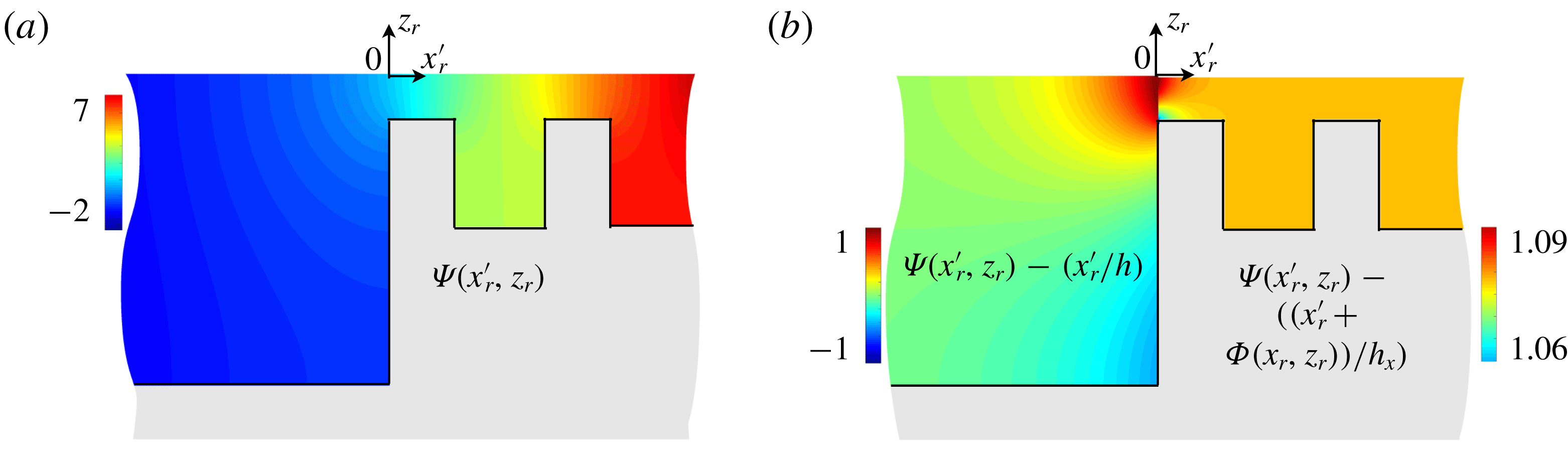
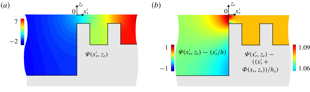
(an example of the field
 $\unicode[STIX]{x1D6F9}$
is given in figure 7). From the limits on
 $\unicode[STIX]{x1D735}_{\mathit{r}}\unicode[STIX]{x1D6F9}$
, we have that
 $$\begin{eqnarray}\displaystyle \left.\begin{array}{@{}ll@{}}\displaystyle \unicode[STIX]{x1D6F9}(x_{\mathit{r}}^{\prime },z_{\mathit{r}})\sim \frac{x_{\mathit{r}}^{\prime }}{h^{\ast }}, & \text{when }x_{\mathit{r}}^{\prime }\rightarrow -\infty ,\\[10.0pt] \displaystyle \unicode[STIX]{x1D6F9}(x_{\mathit{r}}^{\prime },z_{\mathit{r}})\sim \frac{\unicode[STIX]{x1D6F7}(x_{\mathit{r}},z_{\mathit{r}})+x_{\mathit{r}}^{\prime }}{h_{x}^{\ast }}+{\mathcal{B}}, & \text{when }x_{\mathit{r}}^{\prime }\rightarrow +\infty ,\end{array}\right\} & & \displaystyle\end{eqnarray}$$
with
 ${\mathcal{B}}$
a constant. Using these limits in (4.16) and the matching conditions for
 $\unicode[STIX]{x1D713}^{1}$
in (4.6), we get that
 $$\begin{eqnarray}\displaystyle \unicode[STIX]{x1D711}^{1}(0^{+},y,x_{\mathit{r}},z_{\mathit{r}})=D^{0}(y)\left(\frac{\unicode[STIX]{x1D6F7}(x_{\mathit{r}},z_{\mathit{r}})}{h_{x}^{\ast }}+{\mathcal{B}}\right)+\unicode[STIX]{x1D711}^{1}(0^{-},y). & & \displaystyle\end{eqnarray}$$
Expectedly, we recover that
 $\unicode[STIX]{x1D711}_{|x=0^{+}}^{1}$
is periodic with respect
 $x_{\mathit{r}}$
. Eventually, with
 $\langle \unicode[STIX]{x1D6F7}\rangle =0$
, we get the jump in
 $\langle \unicode[STIX]{x1D711}^{1}\rangle$
 $$\begin{eqnarray}\displaystyle \unicode[STIX]{x27E6}\langle \unicode[STIX]{x1D711}^{1}\rangle \unicode[STIX]{x27E7}=\langle \unicode[STIX]{x1D711}^{1}\rangle (0^{+},y)-\unicode[STIX]{x1D711}^{1}(0^{-},y)={\mathcal{B}}\,D^{0}(y), & & \displaystyle\end{eqnarray}$$
(with
 $\langle \unicode[STIX]{x1D711}^{1}\rangle =\unicode[STIX]{x1D711}^{1}$
for
 $x<0$
). At this order, the potential is not continuous anymore and we shall see that the mass flux is not continuous either. To do so, we integrate over
 $\unicode[STIX]{x1D654}_{m}$
the incompressibility relation
 $(\text{div}_{\mathit{r}}\,\boldsymbol{v}^{1}+\unicode[STIX]{x2202}_{y}v_{y}^{0})=0$
from (4.8). With
 $\unicode[STIX]{x2202}_{y}v_{y}^{0}=\unicode[STIX]{x2202}_{yy}\unicode[STIX]{x1D711}^{0}(0,y)$
applying in
 $\unicode[STIX]{x1D654}_{m}$
from (4.15), we get that
 $$\begin{eqnarray}\displaystyle \displaystyle \int _{\unicode[STIX]{x1D654}_{m}}\frac{\unicode[STIX]{x2202}v_{y}^{0}}{\unicode[STIX]{x2202}y}=\left(h^{\ast }\,x_{m}^{\prime }+\int _{0}^{x_{m}^{\prime }}h^{\ast }(x_{\mathit{r}}^{\prime })\,\text{d}x_{r}^{\prime }\right)\,\frac{\unicode[STIX]{x2202}^{2}\unicode[STIX]{x1D711}^{0}}{\unicode[STIX]{x2202}y^{2}}(0,y). & & \displaystyle\end{eqnarray}$$
Next, we use Green’s theorem and we account for the boundary conditions in (4.8) and for the matching condition on
 $\boldsymbol{v}^{1}$
in (4.6) to get that
 $$\begin{eqnarray}\displaystyle \int _{\unicode[STIX]{x1D654}_{m}}\text{div}_{\mathit{r}}\,\boldsymbol{v}^{1}=I^{-}(x_{m}^{\prime })+I^{+}(x_{m}^{\prime }), & & \displaystyle\end{eqnarray}$$
with
 $$\begin{eqnarray}\displaystyle \left.\begin{array}{@{}l@{}}\displaystyle I^{-}(x_{m}^{\prime })=-h^{\ast }\left[u_{x}^{1}-x_{m}^{\prime }\frac{\unicode[STIX]{x2202}u_{x}^{0}}{\unicode[STIX]{x2202}x}\right]_{|x=0^{-}}-x_{m}^{\prime }\unicode[STIX]{x2202}_{tt}\unicode[STIX]{x1D711}^{0}(0,y),\\[12.0pt] \displaystyle I^{+}(x_{m}^{\prime })=\int _{-h^{\ast }(x_{m}^{\prime })}^{0}\left[u_{x}^{1}+x_{m}^{\prime }\frac{\unicode[STIX]{x2202}u_{x}^{0}}{\unicode[STIX]{x2202}x}\right]_{|x=0^{+}}\text{d}z_{\mathit{r}}-x_{m}^{\prime }\unicode[STIX]{x2202}_{tt}\unicode[STIX]{x1D711}^{0}(0,y).\end{array}\right\} & & \displaystyle\end{eqnarray}$$
At
 $x=0^{-}$
, we simply have
 $u_{x}^{n}=\unicode[STIX]{x2202}_{x}\unicode[STIX]{x1D711}^{n}$
,
 $n=0,1$
; next, making use of (3.10) leaves us with
 $$\begin{eqnarray}\displaystyle \displaystyle I^{-}(x_{m}^{\prime })=-h^{\ast }\frac{\unicode[STIX]{x2202}\unicode[STIX]{x1D711}^{1}}{\unicode[STIX]{x2202}x}(0^{-},y)-x_{m}^{\prime }h^{\ast }\;\frac{\unicode[STIX]{x2202}^{2}\unicode[STIX]{x1D711}^{0}}{\unicode[STIX]{x2202}y^{2}}(0,y). & & \displaystyle\end{eqnarray}$$
The term
 $I^{+}$
is evaluated using that
 $u_{x}^{0}=\unicode[STIX]{x2202}_{x}\unicode[STIX]{x1D711}^{0}+\unicode[STIX]{x2202}_{x_{\mathit{r}}}\unicode[STIX]{x1D711}^{1}$
from (3.16) and
 $u_{x}^{1}=\unicode[STIX]{x2202}_{x}\unicode[STIX]{x1D711}^{1}+\unicode[STIX]{x2202}_{x_{\mathit{r}}}\unicode[STIX]{x1D711}^{2}$
from (3.24), with
 $\unicode[STIX]{x1D711}^{1}$
in (3.17) and
 $\unicode[STIX]{x1D711}^{2}$
in (3.25), namely
 $$\begin{eqnarray}\displaystyle \left.\begin{array}{@{}c@{}}\displaystyle u_{x}^{0}=\frac{\unicode[STIX]{x2202}\unicode[STIX]{x1D711}^{0}}{\unicode[STIX]{x2202}x}(\boldsymbol{r})\left(\frac{\unicode[STIX]{x2202}\unicode[STIX]{x1D6F7}}{\unicode[STIX]{x2202}x_{\mathit{r}}}+1\right),\\ \displaystyle u_{x}^{1}=\frac{\unicode[STIX]{x2202}\langle \unicode[STIX]{x1D711}^{1}\rangle }{\unicode[STIX]{x2202}x}(\boldsymbol{r})\left(\frac{\unicode[STIX]{x2202}\unicode[STIX]{x1D6F7}}{\unicode[STIX]{x2202}x_{\mathit{r}}}+1\right)-\frac{\unicode[STIX]{x2202}^{2}\unicode[STIX]{x1D711}^{0}}{\unicode[STIX]{x2202}x^{2}}(\boldsymbol{r})\left(\frac{\unicode[STIX]{x2202}\tilde{\unicode[STIX]{x1D6F7}}}{\unicode[STIX]{x2202}x_{\mathit{r}}}-\unicode[STIX]{x1D6F7}\right)-\frac{\unicode[STIX]{x2202}^{2}\unicode[STIX]{x1D711}^{0}}{\unicode[STIX]{x2202}y^{2}}(\boldsymbol{r})\frac{\unicode[STIX]{x2202}\hat{\unicode[STIX]{x1D6F7}}}{\unicode[STIX]{x2202}x_{\mathit{r}}}.\end{array}\right\} & & \displaystyle\end{eqnarray}$$
It follows that
 $$\begin{eqnarray}\displaystyle \displaystyle I^{+}(x_{m}^{\prime }) & = & \displaystyle h_{x}^{\ast }\,\frac{\unicode[STIX]{x2202}\langle \unicode[STIX]{x1D711}^{1}\rangle }{\unicode[STIX]{x2202}x}(0^{+},y)-\tilde{g}(x_{m}^{\prime })\,\frac{\unicode[STIX]{x2202}^{2}\unicode[STIX]{x1D711}^{0}}{\unicode[STIX]{x2202}x^{2}}(0^{+},y)\nonumber\\ \displaystyle & & \displaystyle -\,{\hat{g}}(x_{m}^{\prime })\,\frac{\unicode[STIX]{x2202}^{2}\unicode[STIX]{x1D711}^{0}}{\unicode[STIX]{x2202}y^{2}}(0,y)-x_{m}^{\prime }\,\langle h^{\ast }\rangle \,\frac{\unicode[STIX]{x2202}^{2}\unicode[STIX]{x1D711}^{0}}{\unicode[STIX]{x2202}y^{2}}(0,y),\end{eqnarray}$$
with the first term obtained using (4.13) and the last term obtained using (3.21). In the above expression, we have defined
 $$\begin{eqnarray}\displaystyle \tilde{g}(x_{m}^{\prime })=\int _{-h^{\ast }(x_{m}^{\prime })}^{0}\left(\frac{\unicode[STIX]{x2202}\tilde{\unicode[STIX]{x1D6F7}}}{\unicode[STIX]{x2202}x_{\mathit{r}}}-\unicode[STIX]{x1D6F7}\right)\text{d}z_{\mathit{r}},\quad {\hat{g}}(x_{m}^{\prime })=\int _{-h^{\ast }(x_{m}^{\prime })}^{0}\frac{\unicode[STIX]{x2202}\hat{\unicode[STIX]{x1D6F7}}}{\unicode[STIX]{x2202}x_{\mathit{r}}}\,\text{d}z_{\mathit{r}}. & & \displaystyle\end{eqnarray}$$
It is shown in appendix A that
 $\tilde{g}(x_{m}^{\prime })=0$
and
 ${\hat{g}}(x_{m}^{\prime })=\int _{x_{0m}}^{x_{m}^{\prime }}(h^{\ast }(x_{\mathit{r}}^{\prime })-\langle h^{\ast }\rangle )\,\text{d}x_{r}^{\prime }$
, with
 $x_{0m}$
any
 $x$
-abscissa where
 $\unicode[STIX]{x2202}_{x_{\mathit{r}}}\tilde{\unicode[STIX]{x1D6F7}}$
and
 $\unicode[STIX]{x2202}_{x_{\mathit{r}}}\hat{\unicode[STIX]{x1D6F7}}$
vanish, hence where
 $\unicode[STIX]{x1D6F7}$
vanishes. With the symmetry of our layers, the zeros of
 $\unicode[STIX]{x1D6F7}$
take place for
 $x_{\mathit{r}}=-1/2,0,1/2$
and for
 $x_{\mathit{r}}^{\prime }\in (x_{0m}-1/2,x_{0m}+1/2)$
, we have
 $x_{\mathit{r}}^{\prime }=x_{0m}+x_{\mathit{r}}$
; it follows that
 $x_{0m}=\unicode[STIX]{x1D6FF}+(m+1)/2$
with
 $m=-1,0,\ldots$
integer and
 $\unicode[STIX]{x1D6FF}$
the distance from the origin to the first half-layer, see figure 6. Eventually, gathering (4.21) and (4.22) along with (4.24) and (4.26) leaves us with
 $$\begin{eqnarray}\displaystyle h_{x}^{\ast }\,\frac{\unicode[STIX]{x2202}\langle \unicode[STIX]{x1D711}^{1}\rangle }{\unicode[STIX]{x2202}x}(0^{+},y)-h^{\ast }\,\frac{\unicode[STIX]{x2202}\unicode[STIX]{x1D711}^{1}}{\unicode[STIX]{x2202}x}(0^{-},y)={\mathcal{C}}\,\frac{\unicode[STIX]{x2202}^{2}\unicode[STIX]{x1D711}^{0}}{\unicode[STIX]{x2202}y^{2}}(0,y), & & \displaystyle\end{eqnarray}$$
with
 $$\begin{eqnarray}\displaystyle {\mathcal{C}}\equiv \int _{0}^{\unicode[STIX]{x1D6FF}}(\langle h^{\ast }\rangle -h^{\ast }(x_{\mathit{r}}^{\prime }))\,\text{d}x_{r}^{\prime }. & & \displaystyle\end{eqnarray}$$
4.3 Final homogenized problem
The final homogenized problem (2.2) along with (2.5) is constructed by considering the potential
 $(\unicode[STIX]{x1D711}^{0}+\unicode[STIX]{x1D700}\,\langle \unicode[STIX]{x1D711}^{1}\rangle )$
. Once coming back to the physical variables using (3.2) along with
 $h^{\ast }=h/\ell$
, equation (3.10) applying for
 $x<0$
, and (3.21), (3.27) applying for
 $x>0$
, gives simply (2.2). Then, from the transmission conditions (4.9), (4.20) and (4.12), (4.28), the potential
 $\unicode[STIX]{x1D711}$
satisfying (2.2) and (2.5) admits the same expansions as
 $(\unicode[STIX]{x1D711}^{0}+\unicode[STIX]{x1D700}\,\langle \unicode[STIX]{x1D711}^{1}\rangle )$
up to
 $O(\unicode[STIX]{x1D700}^{2})$
, hence the same expansion as the potential in the actual problem up to
 $O(\unicode[STIX]{x1D700}^{2})$
. For instance, equations (4.9) and (4.20) provide the relation
 $$\begin{eqnarray}\displaystyle \unicode[STIX]{x27E6}\unicode[STIX]{x1D711}^{0}+\unicode[STIX]{x1D700}\unicode[STIX]{x1D711}^{1}\unicode[STIX]{x27E7}=\unicode[STIX]{x1D700}\,{\mathcal{B}}\,D^{0}=\unicode[STIX]{x1D700}\,{\mathcal{B}}\,\overline{D}+O(\unicode[STIX]{x1D700}^{2}), & & \displaystyle\end{eqnarray}$$
and once coming back to the field with dimensions,
 $\unicode[STIX]{x27E6}\unicode[STIX]{x1D711}\unicode[STIX]{x27E7}={\mathcal{B}}\overline{D}$
. Eventually, we shall refer to the model at first order (that of
 $\unicode[STIX]{x1D711}^{0}$
) the model obtained by setting
 ${\mathcal{B}}={\mathcal{C}}=0$
in (2.5).
5 Discussion on the homogenized problems
The homogenization of the structured ridge with finite extent shows that the two-dimensional wave equation over the structured ridge (2.2) is that of a homogeneous anisotropic medium; it applies at the first and at the second orders. Among the two effective water depths, only
 $h_{x}$
depend on transition effects within the water depth; this holds for a microstructure repeated along
 $x$
only, as we have considered, and the more general case can be found in Rosales & Papanicolaou (Reference Rosales and Papanicolaou1983). Next, the transmission conditions at the first order are the classical continuities of the field and of the normal flux. As a correction to these continuity conditions, the model conducted at second order provides non-intuitive transmission conditions which tell us that these two fields experience a jump at the end boundaries of the ridge, equation (2.5).
The model at first order has a convergence in
 $\unicode[STIX]{x1D700}\propto \unicode[STIX]{x1D714}$
and as such, it will be accurate in some low frequency regime; this is illustrated in appendix D. However, and beyond the convergence, the error of any model at moderate
 $\unicode[STIX]{x1D700}$
values is of practical importance. We shall see that the improvement in the prediction of the scattering properties is significant even at relatively low frequency, especially when the contrast in the water depths is important; this is expected since large contrasts produce strong evanescent fields at the depth discontinuities. In the forthcoming § 6, this will be illustrated, but to gain insights into the importance of the evanescent field, we shall discuss below the variations of the effective parameters entering in the model at the first and second orders for simple layered structure.
5.1 The effective water depth
 $h_{x}$

To begin with, it is shown in § B.1 that
 $h_{x}\leqslant \langle h^{-1}\rangle ^{-1}\leqslant \langle h\rangle =h_{y}$
; this means that the two-step homogenization procedure starting with the use of the shallow water equation overestimates the actual wavelength; this will be illustrated in § 6. Next, the effective depth
 $h_{x}$
depends on the geometry of the unit cell, see figure 4, and as such it depends on the spacing
 $\ell$
which is unusual in effective medium theories; this is a specificity in the context of water waves which do not appear in acoustics and in electromagnetism at leading order. In general,
 $h_{x}$
has to be determined numerically which is not too demanding. However, recalling that
 $h_{x}$
is related to a potential flow problem of a perfect fluid flowing over the ridge with Neumann boundary condition at the free surface, the following trends can be identified:
(i) When
 $\ell$
increases,
 $h_{x}$
tends to
 $\langle h^{-1}\rangle ^{-1}$
since all the dimensions of the periodic cell along
 $z_{\mathit{r}}$
decrease (see figure 4) and the shallow water approximation becomes increasingly valid. Conversely, when
 $\ell$
decreases,
 $h_{x}$
tends to
 $h^{-}$
since the flow cannot enter the dense region of the vertical array, which becomes similar to a flat bottom at depth
 $h^{-}$
(and this remains true for any filling
 $\unicode[STIX]{x1D709}$
).
(ii) The limit
 $\unicode[STIX]{x1D709}=1$
simply corresponds to a ridge of constant water depth
 $h^{-}$
, hence
 $h_{x}=h^{-}$
. The limit
 $\unicode[STIX]{x1D709}\rightarrow 0$
is less trivial since it corresponds to vertical plates (layers of vanishing thickness) for which
 $h_{\mathit{x}0}={h_{x}}_{|\unicode[STIX]{x1D709}=0}$
is unknown. However, once
 $h^{-}\leqslant h_{\mathit{x}0}\leqslant h^{+}$
has been determined, a reasonable approximation of
 $h_{x}$
for any
 $\unicode[STIX]{x1D709}$
value is given by the following form
 $$\begin{eqnarray}\displaystyle h_{x}=\frac{1}{\unicode[STIX]{x1D709}/h^{-}+(1-\unicode[STIX]{x1D709})/h_{\mathit{x}0}}. & & \displaystyle\end{eqnarray}$$
These trends are illustrated in figure 8, where we report
 $h_{x}$
against
 $\unicode[STIX]{x1D709}$
for different spacing
 $\ell$
along with its estimate in (5.1) (using the numerical value of
 $h_{\mathit{x}0}$
); in the reported cases, the agreement is better than 5 %. We also report
 $h_{\mathit{x}0}$
against
 $\ell$
for which we did not find a satisfactory estimate.
Typical variations of
 $h_{x}$
, (a)
 $h_{x}$
against
 $\unicode[STIX]{x1D709}$
for different
 $\ell$
(
 $h^{-}\!=0.05$
,
 $h^{+}=1$
); blue plain lines show
 $h_{x}$
computed numerically and dotted red lines the estimate in (5.1). Dashed grey lines show
 $\langle h^{-1}\rangle ^{-1}$
and
 $\langle h\rangle$
; (b)
 $h_{\mathit{x}0}={h_{x}}_{|\unicode[STIX]{x1D709}=0}$
against
 $\ell$
(
 $h^{-}=0.05$
).

5.2 The effective parameters
$({\mathcal{B}},{\mathcal{C}})$

The effective parameters
 $({\mathcal{B}},{\mathcal{C}})$
entering in the transmission conditions depend on the geometry of the structuration of the ridge at its extremities. We begin with the parameter
 ${\mathcal{C}}$
which has an explicit dependence on this geometry, and use the parametrization
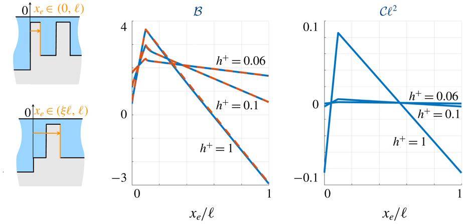
 $x_{\mathit{e}}\in (0,\ell )$
shown in figure 8. For
 $x_{\mathit{e}}=0$
the ridge starts with a vanishing thickness plate at depth
 $h^{-}$
and increasing
 $x_{\mathit{e}}$
produces a shift of the structuration toward the left. From (4.29), it is easy to see that
 ${\mathcal{C}}$
varies following
 $$\begin{eqnarray}\displaystyle {\mathcal{C}}\ell ^{2}=(h^{+}-h^{-})\left\{\begin{array}{@{}ll@{}}\displaystyle (1-\unicode[STIX]{x1D709})\left(x_{\mathit{e}}-\frac{\unicode[STIX]{x1D709}\ell }{2}\right), & x_{\mathit{e}}\in (0,\unicode[STIX]{x1D709}\ell ),\\[10.0pt] \displaystyle \unicode[STIX]{x1D709}\left(-x_{\mathit{e}}+\frac{(1+\unicode[STIX]{x1D709})\ell }{2}\right), & x_{\mathit{e}}\in (\unicode[STIX]{x1D709}\ell ,\ell ).\end{array}\right. & & \displaystyle\end{eqnarray}$$
Unlike
 ${\mathcal{C}}$
,
 ${\mathcal{B}}$
requires the resolution of an elementary problem which is quite involved. Indeed, the problem on
 $\unicode[STIX]{x1D6F9}$
in (4.17) is a problem of potential flow ending on one side with a semi-infinite periodic medium, and this is much more demanding numerically, see chapter 9 in Vinoles (Reference Vinoles2016). Fortunately, the evanescent field that we want to capture is localized in the close vicinity of this ending layer; this means that, in practice, only the ending layer (plus one or two additional layers) can be considered in the numerical resolution and a constant depth can be considered afterwards. It turns out that for the simple layered structure considered here, an accurate approximate expression for
 ${\mathcal{B}}$
is provided which avoids any numerical resolution. To build such an estimate, we make use of two ingredients, (i) the exact result
 ${\mathcal{B}}_{0}$
for ridges of constant immersion depth
 $h_{r}$
provided by Tuck (Reference Tuck1976) (in this case, it is easy to see that
 $\unicode[STIX]{x1D6F7}=0$
is a solution of (3.18) with (3.20); we also get from (3.26) that
 $\tilde{\unicode[STIX]{x1D6F7}}(x_{\mathit{r}},z_{\mathit{r}})=\hat{\unicode[STIX]{x1D6F7}}(x_{\mathit{r}},z_{\mathit{r}})=-z_{\mathit{r}}(z_{\mathit{r}}+2h_{c})/2$
; this is expected since a constant bathymetry does not produce rapid variations of the field. Also expected is the fact that, from (3.17),
 $\unicode[STIX]{x1D711}^{1}(\boldsymbol{r})$
does not depend on
 $(x_{\mathit{r}},z_{\mathit{r}})$
as we have obtained in § 3.1, and from (3.22),
 $h_{x}=h_{y}=h_{r}$
. The transmission conditions at first order are unchanged and at second order simply follow from the problem set in (4.17), with
 $\unicode[STIX]{x1D6F7}=0$
, and
 ${\mathcal{C}}=0$
in agreement with Tuck (Reference Tuck1976))
 $$\begin{eqnarray}\displaystyle {\mathcal{B}}_{0}(\unicode[STIX]{x1D707})=\frac{1}{\unicode[STIX]{x03C0}}\left(\frac{\unicode[STIX]{x1D707}^{2}+1}{\unicode[STIX]{x1D707}}\log \frac{\unicode[STIX]{x1D707}+1}{|\unicode[STIX]{x1D707}-1|}-2\log \frac{4\unicode[STIX]{x1D707}}{|\unicode[STIX]{x1D707}^{2}-1|}\right), & & \displaystyle\end{eqnarray}$$
where
 $\unicode[STIX]{x1D707}=h/h_{r}$
, (ii) explicit lower bounds for
 ${\mathcal{B}}$
, see § B.2. Playing with these two ingredients, an estimate of
 ${\mathcal{B}}$
is found of the form
 $$\begin{eqnarray}\displaystyle {\mathcal{B}}\simeq \left\{\begin{array}{@{}l@{}}\displaystyle \left(x_{\mathit{e}}-\frac{\unicode[STIX]{x1D709}\ell }{2}\right)\left(\frac{1}{h^{-}}-\frac{1}{h_{x}}\right)+{\mathcal{B}}_{0}\left(\frac{h}{h^{-}}\right),\quad x_{\mathit{e}}\in (0,\unicode[STIX]{x1D709}\ell ),\\[10.0pt] \displaystyle (x_{\mathit{e}}-\unicode[STIX]{x1D709}\ell )\left(\frac{1}{h^{+}}-\frac{1}{h_{x}}\right)+\frac{\unicode[STIX]{x1D709}\ell }{2}\left(\frac{1}{h^{-}}-\frac{1}{h_{x}}\right)\\[10.0pt] \quad \displaystyle +\,\hat{{\mathcal{B}}}_{0}+\left({\mathcal{B}}_{0}\left(\frac{h}{h^{-}}\right)-\hat{{\mathcal{B}}}_{0}\right)\text{e}^{-((x_{\mathit{e}}-\unicode[STIX]{x1D709}\ell )/(h^{+}-h^{-}))},\quad x_{\mathit{e}}\in (\unicode[STIX]{x1D709}\ell ,\ell ),\end{array}\right. & & \displaystyle\end{eqnarray}$$
with
 $\hat{{\mathcal{B}}}_{0}={\mathcal{B}}_{0}(h/h^{+})+{\mathcal{B}}_{0}(h^{+}/h^{-})$
. We have accounted for the fact that
 $h^{+}$
and
 $h^{-}$
do not play the same role. Indeed, a first layer at immersion depth
 $h^{-}$
blocks efficiently the flow which does not feel the following layers. On the contrary, when the first layer is at immersion depth
 $h^{+}$
, the effect of the two first layers with decreasing depth immersions have to be accounted for.
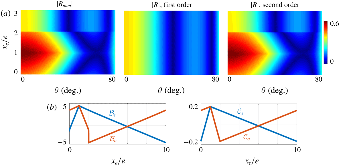
Variations of
 ${\mathcal{B}}$
and
 ${\mathcal{C}}$
against
 $x_{\mathit{e}}$
; we used
 $h=2$
,
 $h^{-}=0.05$
,
 $\unicode[STIX]{x1D709}=0.1$
 $\ell =2$
, and
 $h^{+}=0.06$
, 0.1 and 1. For
 ${\mathcal{B}}$
the plain lines show
 ${\mathcal{B}}$
computed numerically and the dashed lines show the approximate expression in (5.4) (here
 ${\mathcal{B}}_{0}(h/h^{-})=2.10$
).

Typical variations of
 ${\mathcal{B}}$
and
 ${\mathcal{C}}$
against
 $x_{\mathit{e}}$
are shown in figure 9 (in the reported cases, the accuracy of the estimate of
 ${\mathcal{B}}$
in (5.4) is better than 0.2 %). It is worth noting that
 ${\mathcal{B}}$
is discontinuous at
 $x_{\mathit{e}}=0,\ell$
since the two situations are not identical; for
 $x_{\mathit{e}}=0$
the ridge starts on a vanishing thickness plate at immersion depth
 $h^{-}$
while for
 $x_{\mathit{e}}=\ell$
it starts with an entire layer at immersion depth
 $h^{+}$
. Also unusual is the fact that
 ${\mathcal{B}}$
can be negative, while
 ${\mathcal{B}}_{0}\geqslant 0$
for a ridge of constant height.
6 Validation of the homogenized model
In this section, we inspect the validity of the homogenized model in a simple problem of the scattering of an incident plane wave at oblique incidence
 $\unicode[STIX]{x1D703}$
, in the harmonic regime with
 $\text{e}^{-\text{i}\unicode[STIX]{x1D714}t}$
time dependence. To do so, the solution
 $\unicode[STIX]{x1D711}_{\mathit{num}}(\boldsymbol{r},z)$
of the actual three-dimensional problem, and the corresponding scattering coefficients
 $(R_{\mathit{num}},T_{\mathit{num}})$
, are computed numerically using a multimodal method based on matched eigenfunction expansions, see e.g. Maurel et al. (Reference Maurel, Marigo, Cobelli, Petitjeans and Pagneux2017).
6.1 The scattering problem for an incident plane wave
In the homogenized problem, the potential
 $\unicode[STIX]{x1D711}(x,y)$
reads
 $$\begin{eqnarray}\displaystyle \unicode[STIX]{x1D711}(x,y)=\text{e}^{\text{i}k\sin \unicode[STIX]{x1D703}y}\left\{\begin{array}{@{}ll@{}}\displaystyle \text{e}^{\text{i}k_{x}x}+R\text{e}^{-\text{i}k_{x}x}, & x<0,\\ \displaystyle a\text{e}^{\text{i}K_{x}x}+b\text{e}^{-\text{i}K_{x}x}, & 0<x<L,\\ \displaystyle T\text{e}^{\text{i}k_{x}(x-L)}, & L<x,\end{array}\right. & & \displaystyle\end{eqnarray}$$
where
 $k_{x}$
and
 $K_{x}$
satisfy the dispersion relations, from (2.2),
 $\unicode[STIX]{x1D714}^{2}=gh(k_{x}^{2}+k_{y}^{2})$
for
 $x<0$
and
 $x>L$
, and
 $\unicode[STIX]{x1D714}^{2}=g(h_{x}K_{x}^{2}+h_{y}k_{y}^{2})$
for
 $0<x<L$
and in the present case
 $k_{y}=K_{y}=k\sin \unicode[STIX]{x1D703}$
. It is worth noting that such dispersion relations miss the dispersion inherent to water waves. When needed, and in order to inspect the influence of the transmission conditions only, we use the following relations
 $$\begin{eqnarray}\displaystyle \left.\begin{array}{@{}l@{}}\unicode[STIX]{x1D714}^{2}=gk\tan (kh),\\ \unicode[STIX]{x1D714}^{2}=g(K_{x}^{2}h_{x}+K_{y}^{2}h_{y})\tanh (X)/X,\quad X\equiv \sqrt{K_{x}^{2}h_{x}^{2}+K_{y}^{2}h_{y}^{2}},\end{array}\right\} & & \displaystyle\end{eqnarray}$$
where the former is that valid for the flat bathymetry and the latter has been shown to be valid over a layered bathymetry up to relatively high frequencies (Maurel et al.
Reference Maurel, Marigo, Cobelli, Petitjeans and Pagneux2017). The expressions of
 $(R,T,a,b)$
are given in appendix C, where the scattering properties in the homogenized problem are discussed.
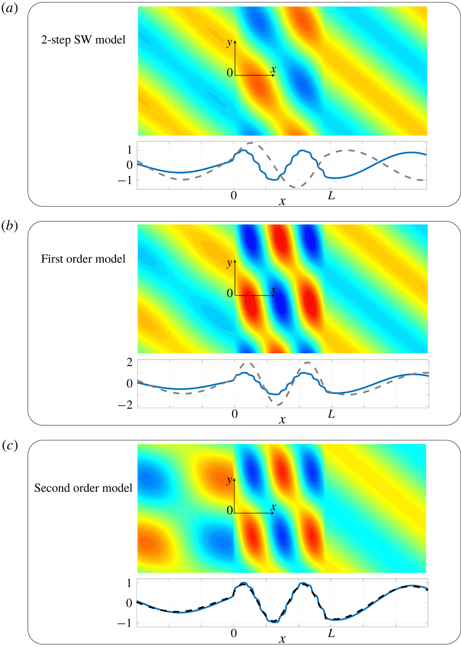
Accuracy of the different models; (a) to (c) report
 $\unicode[STIX]{x1D711}(x,y)$
to be compared with
 $\unicode[STIX]{x1D711}_{\mathit{num}}(x,y,0)$
in figure 1(a) and the profile
 $\unicode[STIX]{x1D711}(x,0)$
(dashed line) along with
 $\unicode[STIX]{x1D711}_{\mathit{num}}(x,0,0)$
(plain blue line). (a) Two-step shallow water model, with
 $h_{x}=\langle h^{-1}\rangle ^{-1}$
and
 $\unicode[STIX]{x27E6}\unicode[STIX]{x1D711}\unicode[STIX]{x27E7}=\unicode[STIX]{x27E6}D\unicode[STIX]{x27E7}=0$
. (b) First-order model, with
 $h_{x}$
corrected, equation (2.3), and
 $\unicode[STIX]{x27E6}\unicode[STIX]{x1D711}\unicode[STIX]{x27E7}=\unicode[STIX]{x27E6}D\unicode[STIX]{x27E7}=0$
). (c) Second-order model, with
 $h_{x}$
corrected and
 $\unicode[STIX]{x27E6}\unicode[STIX]{x1D711}\unicode[STIX]{x27E7}$
,
 $\unicode[STIX]{x27E6}D\unicode[STIX]{x27E7}$
from (2.5).

6.2 Comparison of the different models
To begin with, we come back to the illustration of figure 1. Figure 10 shows the fields
 $\unicode[STIX]{x1D711}(x,y)$
and the profiles
 $\unicode[STIX]{x1D711}(x,0)$
given by the different models. Panel (a) shows the two-step homogenized model using
 $h_{x}=\langle h^{-1}\rangle ^{-1}=0.345$
(
 $h_{y}=0.905$
) and applying the continuities of the surface elevation and of the flux; the error in the field
 $|\unicode[STIX]{x1D711}-\unicode[STIX]{x1D711}_{\mathit{num}}|/|\unicode[STIX]{x1D711}_{\mathit{num}}|$
and on the reflection coefficient
 $|R-R_{\mathit{num}}|/|R_{\mathit{num}}|$
is larger than 100 % and by inspection of the profiles, the error is clearly attributable to an effective wavelength largely overestimated (we have seen that
 $h_{x}<\langle h^{-1}\rangle ^{-1}$
). In panel (b), the homogenized model at first order corrects this drawback by considering the right
 $h_{x}=0.165$
from (2.3) and applying the continuities of the surface elevation and of the flux; although it is visible that the wavenumber over the ridge has been corrected, the scattering properties of the ridge are still not correctly accounted for. The errors remain high with an approximately 50 % discrepancy on the field and 80 % on the reflection coefficient. Eventually in panel (c), the model at second order appears to reproduce with a good accuracy the field and the scattering properties of the ridge, with errors on the field and on
 $R$
of approximately 10 %, which is satisfactory at this relatively high frequency (
 $\unicode[STIX]{x1D700}=\unicode[STIX]{x1D714}\sqrt{h/g}=0.4$
, and decreasing the frequency would produce lower errors). We used the effective parameters
 ${\mathcal{B}}=2.356$
computed numerically (the estimate in (5.4) provides
 ${\mathcal{B}}=2.358$
) and
 ${\mathcal{C}}\ell ^{2}=0.043$
.
6.3 Influence of the ending layers
To illustrate further the influence of the transmission conditions, we shall now focus on the geometry of the ending layers while keeping constant the other parameters. To do so, we set the ridge structuration:
 $h^{+}=1$
,
 $h^{-}=0.05$
,
 $h=2$
,
 $\unicode[STIX]{x1D709}=0.1$
,
 $\ell =4$
and a constant extent
 $L=36.4$
. It follows that in the models at the orders 1 and 2,
 $h_{x}=0.268$
and
 $h_{y}=0.905$
are fixed. Next, the ridge occupies the region
 $x\in (0,L)$
and the form of the first layer is parametrized by
 $x_{\mathit{e}}\in (0,\ell )$
defined in figure 9. Using
 $e=\unicode[STIX]{x1D709}\ell$
as reference length, figure 11 shows the scattering properties of ridges for
 $x_{\mathit{e}}\simeq 0,$
 $e$
and
 $2.5e$
. Specifically, we report (i) the variations of
 $R_{\mathit{num}}$
against
 $\unicode[STIX]{x1D703}$
(plain blue lines) and the corresponding variations of
 $R$
given by the models at the first (dashed grey lines) and at the second orders (black dashed lines), (ii) the wavefields
 $\unicode[STIX]{x1D711}_{\mathit{num}}(x,y,0)$
and
 $\unicode[STIX]{x1D711}(x,y)$
from the model at the second order. The results are given for a frequency
 $\unicode[STIX]{x1D714}\sqrt{h/g}=0.07$
. It is visible that the model at order 2 reproduces accurately the significant variations in the scattering properties of the ridges. These variations are not predicted by the model at first order which see erroneously the same effective structure.
Influence of the layers terminating a ridge of extent
 $L=36.4$
(
 $h^{+}=1$
,
 $h^{-}=0.05$
,
 $h=2$
,
 $\unicode[STIX]{x1D709}=0.1$
and
 $\ell =4$
). The three panels correspond to different layer arrangements at the entrance (see inset, with
 $x_{\mathit{e}}$
defined in figure 9). (a) Reflection coefficient against
 $\unicode[STIX]{x1D703}$
,
 $R_{\mathit{num}}$
from direct numerics (blue plain lines) and
 $R$
from the model at order 1 (dashed grey lines) and from the model at order 2 (dashed black lines). (b) Corresponding fields at incidence
 $\unicode[STIX]{x1D703}=40^{\circ }$
; for comparison,
 $\unicode[STIX]{x1D711}_{\mathit{num}}$
is shown for
 $y>0$
and
 $\unicode[STIX]{x1D711}$
from the model at second order for
 $y<0$
. The frequency is
 $\unicode[STIX]{x1D714}\sqrt{h/g}=0.07$
.
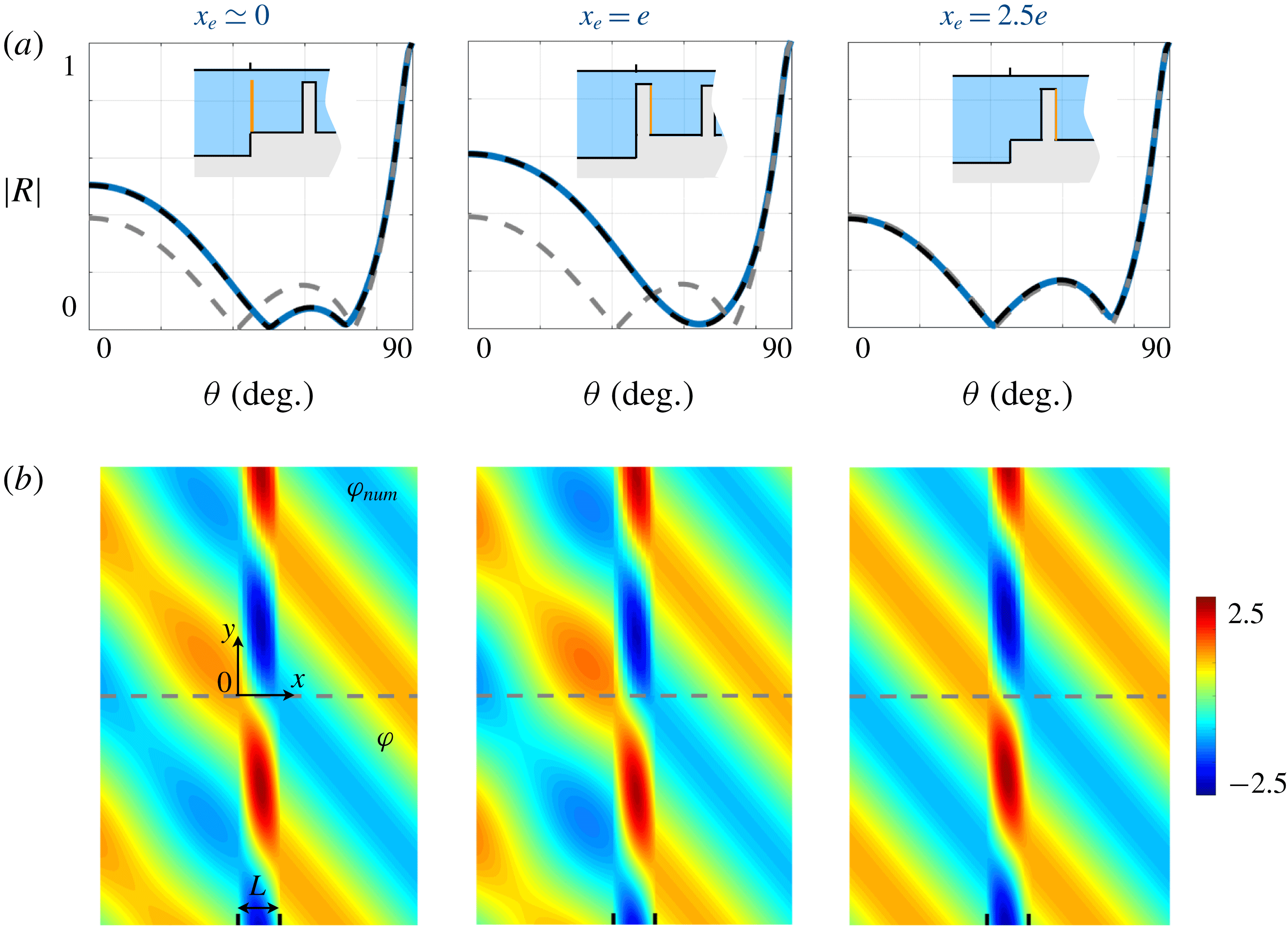
Eventually, figure 12 offers a continuous version of these variations by reporting
 $|R_{\mathit{num}}|$
in colour scale against
 $\unicode[STIX]{x1D703}$
and
 $x_{\mathit{e}}/e$
. The model at second order is accurate with an overall error of approximately 1 %. The corresponding variations of
 $({\mathcal{B}},{\mathcal{C}})$
denoted
 $({\mathcal{B}}_{e},{\mathcal{C}}_{e})$
at the entrance and
 $({\mathcal{B}}_{o},{\mathcal{C}}_{o})$
at the exit are reported and allow us to interpret the observed variations. For
 $x_{\mathit{e}}\in (0,e)$
the parameters vary rapidly, resulting in rapid variations of the scattering properties. Due to the symmetry of the ridge,
 $x_{\mathit{e}}\in (e,2e)$
exchanges the role of the entrance and exit, hence
 $R_{\mathit{num}}$
follows the reverse course. For
 $x_{\mathit{e}}=2e=0.8$
,
 ${\mathcal{B}}_{o}$
experiences a jump corresponding to the disappearance of a layer at immersion depth
 $h^{-}$
. Eventually, for
 $x_{\mathit{e}}>2e$
, the end boundaries of the ridge are formed by a layer at immersion depth
 $h^{+}$
which produces
 ${\mathcal{B}}_{o}\simeq -{\mathcal{B}}_{e}$
and
 ${\mathcal{C}}_{o}\simeq -{\mathcal{C}}_{e}$
. Inspecting
 $R$
in (C 6) shows that this produces the cancellation of the dominant corrections in
 ${\mathcal{B}}(kh)$
,
 ${\mathcal{C}}(kh)$
; thus, although each extremity of the ridge is the place of significant transition effects, their collective effect tends to cancel. As a consequence, the scattering properties for
 $x_{\mathit{e}}>2e$
are correctly described by the model at first order.
(a) Variations of
 $R_{\mathit{num}}$
and
 $R$
in the model at first and second orders against
 $x_{\mathit{e}}$
and
 $\unicode[STIX]{x1D703}$
in colour scale. (b) Corresponding variations of the parameters (
 ${\mathcal{B}},{\mathcal{C}}$
) against
 $x_{\mathit{e}}$
(index
 $e$
refers to the ridge entrance at
 $o$
to the ridge exit).

7 Concluding remarks
In this work, we study the problem of the scattering of water waves by a structured ridge of finite extent. Our work focuses on non-intuitive effective transmission conditions which complement the effective two-dimensional wave equation derived in Rosales & Papanicolaou (Reference Rosales and Papanicolaou1983) and recently validated experimentally in Maurel et al. (Reference Maurel, Marigo, Cobelli, Petitjeans and Pagneux2017). Although such transmission conditions have been derived for trenches and ridges with constant immersion depth, they have not been considered for periodically structured devices as envisaged recently by the community of metamaterials. In the present study, we restricted ourselves to structurations with symmetries which produce substantial simplifications in the derivation of the effective model conducted at second order with respect to a small parameter which is a measure of the shallowness regime and of the subwavelength character of the structuration. While extension of the present work is straightforward for non-symmetric structurations, the complexity of the resulting model would be quite cumbersome since it would involve much more effective parameters both in the effective wave equation and in the transmission conditions. In our opinion, more promising extensions concern the homogenization of floating or partially submerged structured devices which have practical applications beyond the shallow water regime; as such, metamaterial devices in the deep ocean can be sought. Also of interest is to include more realistic effects, such as the viscosity of the fluid and the nonlinearities of the waves, or coupling effects accounting for the possible elasticity of the devices.
Appendix A. Useful relations
In this section, we define
 $\unicode[STIX]{x1D6FA}_{x}$
the subdomain of
 $\unicode[STIX]{x1D6FA}$
restricted to
 $(0,x_{\mathit{r}})$
along the horizontal direction (and
 $x_{\mathit{r}}\in (-1/2,1/2)$
).
A.1 Property on
$\unicode[STIX]{x1D6F7}$

We have defined
 $h_{x}^{\ast }$
in (3.22) and in (4.13), with
 $\unicode[STIX]{x1D6F7}$
satisfying (3.18). Integrating
 $\unicode[STIX]{x1D6FB}_{\mathit{r}}^{2}(\unicode[STIX]{x1D6F7}+x_{\mathit{r}})=0$
over
 $\unicode[STIX]{x1D6FA}_{x}$
and accounting for the boundary conditions
 $\unicode[STIX]{x2202}_{z_{\mathit{r}}}\unicode[STIX]{x1D6F7}=0$
at
 $z_{\mathit{r}}=0$
and
 $\unicode[STIX]{x1D735}_{\mathit{r}}(\unicode[STIX]{x1D6F7}+x_{\mathit{r}})\boldsymbol{\cdot }\boldsymbol{n}_{|\unicode[STIX]{x1D6E4}}=0$
, we easily get that
 $$\begin{eqnarray}\displaystyle \int _{-h^{\ast }(x_{\mathit{r}})}^{0}\left(\frac{\unicode[STIX]{x2202}\unicode[STIX]{x1D6F7}}{\unicode[STIX]{x2202}x_{\mathit{r}}}(x_{\mathit{r}},z_{\mathit{r}})+1\right)\text{d}z_{\mathit{r}}=\int _{-h^{\ast }(0)}^{0}\left(\frac{\unicode[STIX]{x2202}\unicode[STIX]{x1D6F7}}{\unicode[STIX]{x2202}x_{\mathit{r}}}(0,z_{\mathit{r}})+1\right)\text{d}z_{\mathit{r}}, & & \displaystyle\end{eqnarray}$$
hence it is independent of
 $x_{\mathit{r}}\in (-1/2,1/2)$
. It immediately follows that
 $$\begin{eqnarray}\displaystyle \int _{-h^{\ast }(x_{\mathit{r}})}^{0}\left(\frac{\unicode[STIX]{x2202}\unicode[STIX]{x1D6F7}}{\unicode[STIX]{x2202}x_{\mathit{r}}}(x_{\mathit{r}},z_{\mathit{r}})+1\right)\text{d}z_{\mathit{r}}=h_{x}^{\ast }. & & \displaystyle\end{eqnarray}$$
A.2 Property on
$\tilde{g}(x_{\mathit{r}})$

Making use of
 $\text{div}(\unicode[STIX]{x1D6F7}\boldsymbol{e}_{\mathit{x}})=\unicode[STIX]{x2202}_{x_{\mathit{r}}}\unicode[STIX]{x1D6F7}$
, we write for
 $\tilde{\unicode[STIX]{x1D6F7}}$
satisfying (3.26) that
 $\text{div}(\unicode[STIX]{x1D735}_{\mathit{r}}\tilde{\unicode[STIX]{x1D6F7}}-\unicode[STIX]{x1D6F7}\boldsymbol{e}_{\mathit{x}})=\unicode[STIX]{x2202}_{x_{\mathit{r}}}\unicode[STIX]{x1D6F7}+1$
, which we integrate over
 $\unicode[STIX]{x1D6FA}_{x}$
. We get
 $$\begin{eqnarray}\displaystyle \displaystyle \int _{\unicode[STIX]{x1D6FA}_{x}}\left(\frac{\unicode[STIX]{x2202}\unicode[STIX]{x1D6F7}}{\unicode[STIX]{x2202}x_{\mathit{r}}}+1\right)=\int _{\unicode[STIX]{x2202}\unicode[STIX]{x1D6FA}_{x}}(\unicode[STIX]{x1D735}_{\mathit{r}}\tilde{\unicode[STIX]{x1D6F7}}-\unicode[STIX]{x1D6F7}\boldsymbol{e}_{\mathit{x}})\boldsymbol{\cdot }\boldsymbol{n}, & & \displaystyle\end{eqnarray}$$
where the second equality is obtained using Green’s theorem. It is now sufficient to account for the boundary condition
 $\unicode[STIX]{x2202}_{z_{\mathit{r}}}\tilde{\unicode[STIX]{x1D6F7}}_{|z_{\mathit{r}}=0}=h_{x}$
and
 $\unicode[STIX]{x1D735}_{\mathit{r}}\tilde{\unicode[STIX]{x1D6F7}}\boldsymbol{\cdot }\boldsymbol{n}_{|\unicode[STIX]{x1D6E4}}=\unicode[STIX]{x1D6F7}\,\boldsymbol{e}_{\mathit{x}}\boldsymbol{\cdot }\boldsymbol{n}_{|\unicode[STIX]{x1D6E4}}$
to get that
 $$\begin{eqnarray}\displaystyle \int _{\unicode[STIX]{x2202}\unicode[STIX]{x1D6FA}_{x}}(\unicode[STIX]{x1D735}_{\mathit{r}}\tilde{\unicode[STIX]{x1D6F7}}-\unicode[STIX]{x1D6F7}\boldsymbol{e}_{\mathit{x}})\boldsymbol{\cdot }\boldsymbol{n}=h_{x}^{\ast }\,x_{\mathit{r}}+\tilde{g}(x_{\mathit{r}})-\tilde{g}(0), & & \displaystyle\end{eqnarray}$$
where
 $$\begin{eqnarray}\displaystyle \tilde{g}(x_{\mathit{r}})\equiv \int _{-h^{\ast }(x_{\mathit{r}})}^{0}\left(\frac{\unicode[STIX]{x2202}\tilde{\unicode[STIX]{x1D6F7}}}{\unicode[STIX]{x2202}x_{\mathit{r}}}(x_{\mathit{r}},z_{\mathit{r}})-\unicode[STIX]{x1D6F7}(x_{\mathit{r}},z_{\mathit{r}})\right)\text{d}z_{\mathit{r}}. & & \displaystyle\end{eqnarray}$$
Making now use of (A 2) in (A 3) leaves us with
 $\tilde{g}(x_{\mathit{r}})=\tilde{g}(0)$
being independent of
 $x_{\mathit{r}}$
. In the case of symmetric sea bed shape,
 $\unicode[STIX]{x2202}_{x_{\mathit{r}}}\tilde{\unicode[STIX]{x1D6F7}}$
and
 $\unicode[STIX]{x1D6F7}$
are odd with respect to
 $x_{\mathit{r}}$
, hence
 $\tilde{g}(0)=0=\tilde{g}(x_{\mathit{r}})$
.
It is worth noting that extending
 $\tilde{\unicode[STIX]{x1D6F7}}$
and
 $\unicode[STIX]{x1D6F7}$
in the whole space would produce the same result as long as the origin, say
 $0_{m}$
, corresponds to a zero of
 $\unicode[STIX]{x1D6F7}$
(hence a zero of
 $\unicode[STIX]{x2202}_{x_{\mathit{r}}}\tilde{\unicode[STIX]{x1D6F7}}$
).
A.3 Property on
${\hat{g}}(x_{\mathit{r}})$

Again, we use that
 $\hat{\unicode[STIX]{x1D6F7}}$
satisfies (3.26), and integrating
 $\unicode[STIX]{x1D6FB}_{\mathit{r}}^{2}\hat{\unicode[STIX]{x1D6F7}}=1$
over
 $\unicode[STIX]{x1D6FA}_{x}$
leaves us with
 $$\begin{eqnarray}\displaystyle \int _{0}^{x_{\mathit{r}}}h^{\ast }(x^{\prime })\,\text{d}x^{\prime }=\int _{\unicode[STIX]{x2202}\unicode[STIX]{x1D6FA}_{x}}\unicode[STIX]{x1D735}_{\mathit{r}}\hat{\unicode[STIX]{x1D6F7}}\boldsymbol{\cdot }\boldsymbol{n}. & & \displaystyle\end{eqnarray}$$
The boundary conditions
 $\unicode[STIX]{x2202}_{z}\hat{\unicode[STIX]{x1D6F7}}_{|z_{\mathit{r}}=0}=\langle h^{\ast }\rangle$
and
 $\unicode[STIX]{x1D735}_{\mathit{r}}\hat{\unicode[STIX]{x1D6F7}}\boldsymbol{\cdot }\boldsymbol{n}_{|\unicode[STIX]{x1D6E4}}=0$
are used to get that
 $$\begin{eqnarray}\displaystyle \int _{\unicode[STIX]{x2202}\unicode[STIX]{x1D6FA}_{x}}\unicode[STIX]{x1D735}_{\mathit{r}}\hat{\unicode[STIX]{x1D6F7}}\boldsymbol{\cdot }\boldsymbol{n}=\langle h^{\ast }\rangle \,x_{\mathit{r}}+{\hat{g}}(x_{\mathit{r}})-{\hat{g}}(0), & & \displaystyle\end{eqnarray}$$
where
 $$\begin{eqnarray}\displaystyle {\hat{g}}(x_{\mathit{r}})=\int _{-h^{\ast }(x_{\mathit{r}})}^{0}\frac{\unicode[STIX]{x2202}\hat{\unicode[STIX]{x1D6F7}}}{\unicode[STIX]{x2202}x_{\mathit{r}}}(x_{\mathit{r}},z_{\mathit{r}})\,\text{d}z_{\mathit{r}}. & & \displaystyle\end{eqnarray}$$
Eventually, for symmetric sea bed shape,
 ${\hat{g}}(0)=0$
which provides
 $$\begin{eqnarray}\displaystyle {\hat{g}}(x_{\mathit{r}})=\int _{0}^{x_{\mathit{r}}}(h^{\ast }(x^{\prime })-\langle h^{\ast }\rangle )\,\text{d}x^{\prime }. & & \displaystyle\end{eqnarray}$$
Appendix B. Some bounds of the effective parameters
B.1 Upper bound of
$h_{x}$

We shall use a principle of energy minimization to show that
 $h_{x}\leqslant \langle h^{-1}\rangle ^{-1}\leqslant \langle h\rangle$
. To avoid heavy notation, we use in this section
 $\ell =1$
. From (3.18), we have that for any field
 $\tilde{\unicode[STIX]{x1D6F7}}$
 $$\begin{eqnarray}\displaystyle 0=\int _{\unicode[STIX]{x1D6FA}}\tilde{\unicode[STIX]{x1D6F7}}\unicode[STIX]{x0394}\unicode[STIX]{x1D6F7}=-\int _{\unicode[STIX]{x1D6FA}}\unicode[STIX]{x1D735}\tilde{\unicode[STIX]{x1D6F7}}\boldsymbol{\cdot }\unicode[STIX]{x1D735}\unicode[STIX]{x1D6F7}-\int _{\unicode[STIX]{x1D6FA}}\unicode[STIX]{x2202}_{x_{\mathit{r}}}\tilde{\unicode[STIX]{x1D6F7}}. & & \displaystyle\end{eqnarray}$$
The Dirichlet principle tells us that for any admissible
 $\tilde{\unicode[STIX]{x1D6F7}}$
being continuous and square integrable, we have
 $$\begin{eqnarray}\displaystyle E(\unicode[STIX]{x1D6F7})={\textstyle \frac{1}{2}}(h_{x}-\langle h\rangle )\leqslant E(\tilde{\unicode[STIX]{x1D6F7}}),\quad \text{with }E(\tilde{\unicode[STIX]{x1D6F7}})=\int _{\unicode[STIX]{x1D6FA}}({\textstyle \frac{1}{2}}|\unicode[STIX]{x1D735}\tilde{\unicode[STIX]{x1D6F7}}|^{2}+\unicode[STIX]{x2202}_{x_{\mathit{r}}}\tilde{\unicode[STIX]{x1D6F7}}), & & \displaystyle\end{eqnarray}$$
where
 $E(\unicode[STIX]{x1D6F7})$
has been obtained using that
 $|\unicode[STIX]{x1D735}\unicode[STIX]{x1D6F7}|^{2}=\langle h\rangle -h_{x}$
, from (B 1) (with
 $\tilde{\unicode[STIX]{x1D6F7}}=\unicode[STIX]{x1D6F7}$
). If one chooses
 $\tilde{\unicode[STIX]{x1D6F7}}=0$
, we get that
 $h_{x}\leqslant \langle h\rangle$
but we want more. Hence we choose
 $\tilde{\unicode[STIX]{x1D6F7}}(x_{\mathit{r}},z_{\mathit{r}})=f(x_{\mathit{r}})$
with
 $f(x_{\mathit{r}})$
an odd function of
 $x_{\mathit{r}}\in (-1/2,1/2)$
with
 $f(x_{\mathit{r}})=ax_{\mathit{r}}/\unicode[STIX]{x1D709}$
, for
 $x_{\mathit{r}}\in (0,\unicode[STIX]{x1D709}/2)$
and
 $f(x_{\mathit{r}})=a(x_{\mathit{r}}-1/2)/(\unicode[STIX]{x1D709}-1),$
for
 $x_{\mathit{r}}\in (\unicode[STIX]{x1D709}/2,1/2)$
, and at this stage
 $a$
is a free parameter. It follows that
 $$\begin{eqnarray}\displaystyle E(\tilde{\unicode[STIX]{x1D6F7}})=\frac{a^{2}}{2}\left(\frac{h^{-}}{\unicode[STIX]{x1D709}}+\frac{h^{+}}{1-\unicode[STIX]{x1D709}}\right)-a(h^{+}-h^{-}), & & \displaystyle\end{eqnarray}$$
which is minimum for
 $a=(h^{+}-h^{-})/(h^{-}/\unicode[STIX]{x1D709}+h^{+}/(1-\unicode[STIX]{x1D709}))$
, resulting in
 $$\begin{eqnarray}\displaystyle E(\tilde{\unicode[STIX]{x1D6F7}})=-\frac{1}{2}\frac{(h^{+}-h^{-})^{2}}{\displaystyle \frac{h^{-}}{\unicode[STIX]{x1D709}}+\frac{h^{+}}{1-\unicode[STIX]{x1D709}}}. & & \displaystyle\end{eqnarray}$$
It follows from (B 2) that
 $$\begin{eqnarray}\displaystyle h_{x}\leqslant \langle h\rangle -\frac{(h^{+}-h^{-})^{2}}{\displaystyle \frac{h^{-}}{\unicode[STIX]{x1D709}}+\frac{h^{+}}{1-\unicode[STIX]{x1D709}}}=\langle h^{-1}\rangle ^{-1}, & & \displaystyle\end{eqnarray}$$
from which
 $$\begin{eqnarray}\displaystyle h_{x}\leqslant \langle h^{-1}\rangle ^{-1}\leqslant \langle h\rangle , & & \displaystyle\end{eqnarray}$$
which shows that the actual effective water depth
 $h_{x}$
is smaller than the arithmetic and geometric averages predicted within the shallow water approximation.
B.2 Lower bound of
${\mathcal{B}}$

To get a simple lower bound for
 ${\mathcal{B}}$
, it is sufficient to use the so-called Dirichlet principle, which allows us to set the problem (4.17) as a problem of energy minimization. To do so, we start by defining
 $$\begin{eqnarray}\displaystyle \left.\begin{array}{@{}ll@{}}\displaystyle \unicode[STIX]{x1D6F9}_{\mathit{s}}(x_{\mathit{r}}^{\prime },z_{\mathit{r}})=\unicode[STIX]{x1D6F9}(x_{\mathit{r}}^{\prime },z_{\mathit{r}})-\frac{x_{\mathit{r}}^{\prime }}{h}, & x_{\mathit{r}}^{\prime }<0,\\[10.0pt] \displaystyle \unicode[STIX]{x1D6F9}_{\mathit{s}}(x_{\mathit{r}}^{\prime },z_{\mathit{r}})=\unicode[STIX]{x1D6F9}(x_{\mathit{r}}^{\prime },z_{\mathit{r}})-\frac{\unicode[STIX]{x1D6F7}(x_{\mathit{r}},z_{\mathit{r}})+x_{\mathit{r}}^{\prime }}{h_{x}}, & x_{\mathit{r}}^{\prime }>0,\end{array}\right\} & & \displaystyle\end{eqnarray}$$
hence
 $\unicode[STIX]{x1D735}\unicode[STIX]{x1D6F9}_{\mathit{s}}$
is square integrable, with
 $\unicode[STIX]{x27E6}\unicode[STIX]{x1D6F9}_{\mathit{s}}\unicode[STIX]{x27E7}=-\unicode[STIX]{x1D6F7}_{|x_{\mathit{r}}^{\prime }=0}/h_{x}$
and
 $\unicode[STIX]{x1D6F9}_{\mathit{s}}(+\infty ,z_{\mathit{r}})-\unicode[STIX]{x1D6F9}_{\mathit{s}}(-\infty ,z_{\mathit{r}})={\mathcal{B}}$
. Now, it is straightforward to get that
 $\unicode[STIX]{x1D6F9}_{\mathit{s}}$
satisfies the following problem
 $$\begin{eqnarray}\displaystyle & \displaystyle {\mathcal{E}}(\unicode[STIX]{x1D6F9}_{\mathit{s}})\leqslant {\mathcal{E}}(\unicode[STIX]{x1D6F9}^{\ast }), & \displaystyle\end{eqnarray}$$
 $$\begin{eqnarray}\displaystyle & \displaystyle {\mathcal{E}}(\unicode[STIX]{x1D6F9}^{\ast })=\int _{\unicode[STIX]{x1D6FA}}\frac{1}{2}|\unicode[STIX]{x1D735}\unicode[STIX]{x1D6F9}^{\ast }|^{2}+\frac{1}{h}\int _{\unicode[STIX]{x1D6FA}^{-}}\frac{\unicode[STIX]{x2202}\unicode[STIX]{x1D6F9}^{\ast }}{\unicode[STIX]{x2202}x_{\mathit{r}}}+\frac{1}{h_{x}}\int _{\unicode[STIX]{x1D6FA}^{+}}\left(\frac{\unicode[STIX]{x2202}\unicode[STIX]{x1D6F9}^{\ast }}{\unicode[STIX]{x2202}x_{\mathit{r}}}+\unicode[STIX]{x1D735}\unicode[STIX]{x1D6F9}^{\ast }\boldsymbol{\cdot }\unicode[STIX]{x1D735}\unicode[STIX]{x1D6F7}\right)-{\mathcal{B}}^{\ast },\quad & \displaystyle\end{eqnarray}$$
 ${\mathcal{B}}^{\ast }=\unicode[STIX]{x1D6F9}^{\ast }(+\infty ,z_{\mathit{r}})-\unicode[STIX]{x1D6F9}^{\ast }(-\infty ,z_{\mathit{r}})$
, and where the
 $\unicode[STIX]{x1D6F9}^{\ast }$
is any admissible field, specifically whose gradient is square integrable and which satisfies
 $\unicode[STIX]{x27E6}\unicode[STIX]{x1D6F9}^{\ast }\unicode[STIX]{x27E7}=-\unicode[STIX]{x1D6F7}_{|x_{\mathit{r}}^{\prime }=0}/h_{x}$
. To establish the lower bound for
 ${\mathcal{B}}$
, it remains to derive
 ${\mathcal{E}}(\unicode[STIX]{x1D6F9}_{\mathit{s}})$
and to choose an admissible field
 $\unicode[STIX]{x1D6F9}^{\ast }$
. The energy associated with
 $\unicode[STIX]{x1D6F9}_{\mathit{s}}$
reads as
 $$\begin{eqnarray}\displaystyle {\mathcal{E}}(\unicode[STIX]{x1D6F9}_{\mathit{s}})=\frac{1}{2h_{x}^{2}}\int _{0}^{\unicode[STIX]{x1D6FF}}\,\text{d}x_{r}^{\prime }\int \text{d}z_{\mathit{r}}\,\left(|\unicode[STIX]{x1D735}\unicode[STIX]{x1D6F7}|^{2}+\frac{\unicode[STIX]{x2202}\unicode[STIX]{x1D6F7}}{\unicode[STIX]{x2202}x_{\mathit{r}}}\right)-\frac{{\mathcal{B}}}{2}. & & \displaystyle\end{eqnarray}$$
(i) For a starting layer with water depth
 $h^{-}$
, we focus on the first layer only. We choose
 $$\begin{eqnarray}\displaystyle \unicode[STIX]{x1D6F9}^{\ast }(x_{\mathit{r}},z_{\mathit{r}})=\left\{\begin{array}{@{}ll@{}}0, & x_{\mathit{r}}<0,\\ \displaystyle a\frac{x_{\mathit{r}}}{\unicode[STIX]{x1D6FF}}-\frac{\unicode[STIX]{x1D6F7}(x_{\mathit{r}},z_{\mathit{r}})}{h_{x}}, & 0<x_{\mathit{r}}<\unicode[STIX]{x1D6FF},\\ a, & \unicode[STIX]{x1D6FF}<x_{\mathit{r}},\end{array}\right. & & \displaystyle\end{eqnarray}$$
and at this stage
 $a$
is a free parameter. Remember that, by definition of
 $\unicode[STIX]{x1D6FF}$
,
 $\unicode[STIX]{x1D6F7}(\unicode[STIX]{x1D6FF},z_{\mathit{r}})=0$
, which ensures that
 $\unicode[STIX]{x1D6F9}^{\ast }$
is continuous everywhere except at
 $x_{\mathit{r}}=0$
. Inserting this form of
 $\unicode[STIX]{x1D6F9}^{\ast }$
, and accounting for (A 2), we obtain
 $$\begin{eqnarray}\displaystyle {\mathcal{E}}(\unicode[STIX]{x1D6F9}^{\ast })=\frac{h^{-}}{2\unicode[STIX]{x1D6FF}}\,a^{2}+\left(\frac{h^{-}}{h_{x}}-1\right)\left(a+\frac{\unicode[STIX]{x1D6FF}}{h_{x}}\right)-\frac{1}{2h_{x}^{2}}\int _{0}^{\unicode[STIX]{x1D6FF}}\,\text{d}x_{r}^{\prime }\int \text{d}z_{\mathit{r}}\,|\unicode[STIX]{x1D735}\unicode[STIX]{x1D6F7}|^{2}, & & \displaystyle\end{eqnarray}$$
while
 $$\begin{eqnarray}\displaystyle {\mathcal{E}}(\unicode[STIX]{x1D6F9}_{\mathit{s}})=\frac{\unicode[STIX]{x1D6FF}}{2h_{x}}\left(\frac{h^{-}}{h_{x}}-1\right)-\frac{{\mathcal{B}}}{2}-\frac{1}{2h_{x}^{2}}\int _{0}^{\unicode[STIX]{x1D6FF}}\,\text{d}x_{r}^{\prime }\int \text{d}z_{\mathit{r}}\,|\unicode[STIX]{x1D735}\unicode[STIX]{x1D6F7}|^{2}. & & \displaystyle\end{eqnarray}$$
It follows that the principle of energy minimization reduces to
 $$\begin{eqnarray}\displaystyle {\mathcal{B}}\geqslant -\frac{h^{-}}{\unicode[STIX]{x1D6FF}}\,a^{2}-2\left(\frac{h^{-}}{h_{x}}-1\right)a-\left(\frac{h^{-}}{h_{x}}-1\right)\frac{\unicode[STIX]{x1D6FF}}{h_{x}}, & & \displaystyle\end{eqnarray}$$
for any
 $a$
, and the maximum with respect to
 $a$
of the right-hand side term is reached for
 $a=(1/h_{x}-1/h^{-})\unicode[STIX]{x1D6FF}$
, leading to
 $$\begin{eqnarray}\displaystyle {\mathcal{B}}\geqslant \unicode[STIX]{x1D6FF}\left(\frac{1}{h^{-}}-\frac{1}{h_{x}}\right), & & \displaystyle\end{eqnarray}$$
which is used in (5.4), with
 $\unicode[STIX]{x1D6FF}=x_{\mathit{e}}-\unicode[STIX]{x1D709}\ell /2$
.
(ii) When the first layer is associated with water depth
 $h^{+}$
, we want to account for the two first layers; hence we set
 $\unicode[STIX]{x1D6FF}=\hat{\unicode[STIX]{x1D6FF}}+\unicode[STIX]{x1D709}\ell /2$
, and we choose
 $$\begin{eqnarray}\displaystyle \unicode[STIX]{x1D6F9}^{\ast }(x_{\mathit{r}},z_{\mathit{r}})=\left\{\begin{array}{@{}ll@{}}0, & x_{\mathit{r}}<0,\\ \displaystyle b\frac{x_{\mathit{r}}}{\hat{\unicode[STIX]{x1D6FF}}}-\frac{\unicode[STIX]{x1D6F7}(x_{\mathit{r}},z_{\mathit{r}})}{h_{x}}, & 0<x_{\mathit{r}}<\hat{\unicode[STIX]{x1D6FF}},\\[10.0pt] \displaystyle (a-b)\frac{x_{\mathit{r}}-\hat{\unicode[STIX]{x1D6FF}}}{\unicode[STIX]{x1D709}\ell /2}+b-\frac{\unicode[STIX]{x1D6F7}(x_{\mathit{r}},z_{\mathit{r}})}{h_{x}}, & \hat{\unicode[STIX]{x1D6FF}}<x_{\mathit{r}}<\unicode[STIX]{x1D6FF},\\ a, & x_{\mathit{r}}>\unicode[STIX]{x1D6FF},\end{array}\right. & & \displaystyle\end{eqnarray}$$
with
 $(a,b)$
free parameters. It is easy to see that the problem can be set as a combination of two problems of minimization on
 $a$
and
 $b$
independently, resulting in
 $$\begin{eqnarray}\displaystyle {\mathcal{B}}\geqslant \hat{\unicode[STIX]{x1D6FF}}\left(\frac{1}{h^{+}}-\frac{1}{h_{x}}\right)+\frac{\unicode[STIX]{x1D709}\ell }{2}\left(\frac{1}{h^{-}}-\frac{1}{h_{x}}\right), & & \displaystyle\end{eqnarray}$$
which is used in (5.4), with
 $\hat{\unicode[STIX]{x1D6FF}}=x_{\mathit{e}}-\unicode[STIX]{x1D709}\ell$
.
Appendix C. Scattering properties
Here, we solve the full scattering problem for incident right-going and left-going waves of amplitudes
 $(\unicode[STIX]{x1D711}^{\mathit{inc},-},\unicode[STIX]{x1D711}^{\mathit{inc},+})$
. The solution reads as
 $$\begin{eqnarray}\displaystyle \unicode[STIX]{x1D711}(x,y)=\text{e}^{\text{i}k\sin \unicode[STIX]{x1D703}y}\left\{\begin{array}{@{}ll@{}}\displaystyle \unicode[STIX]{x1D711}^{\mathit{inc},+}\text{e}^{\text{i}k_{x}x}+\unicode[STIX]{x1D711}^{-}\text{e}^{-\text{i}k_{x}x}, & x<0,\\[2.0pt] \displaystyle a\text{e}^{\text{i}K_{x}x}+b\text{e}^{-\text{i}K_{x}x}, & 0<x<L,\\ \displaystyle \unicode[STIX]{x1D711}^{+}\text{e}^{\text{i}k_{x}(x-L)}+\unicode[STIX]{x1D711}^{\mathit{inc},-}\text{e}^{-\text{i}k_{x}(x-L)}, & L<x.\end{array}\right. & & \displaystyle\end{eqnarray}$$
Applying the jump conditions at
 $x=0$
and
 $x=L$
leaves us with the relations involving the local scattering coefficients
 $(t_{\mathit{e,o}}^{\pm },r_{\mathit{e,o}}^{\pm })$
of the form
 $$\begin{eqnarray}\displaystyle \left(\begin{array}{@{}c@{}}a\\ \unicode[STIX]{x1D711}^{-}\end{array}\right)=\left(\begin{array}{@{}cc@{}}t_{\mathit{e}}^{+} & r_{\mathit{e}}^{-}\\ r_{\mathit{e}}^{+} & t_{\mathit{e}}^{-}\end{array}\right)\left(\begin{array}{@{}c@{}}\unicode[STIX]{x1D711}^{\mathit{inc},+}\\ b\end{array}\right),\quad \left(\begin{array}{@{}c@{}}\unicode[STIX]{x1D711}^{+}\\ b\text{e}^{-\text{i}K_{x}L}\end{array}\right)=\left(\begin{array}{@{}cc@{}}t_{\mathit{o}}^{+} & r_{\mathit{o}}^{-}\\ r_{\mathit{o}}^{+} & t_{\mathit{o}}^{-}\end{array}\right)\left(\begin{array}{@{}c@{}}a\text{e}^{\text{i}K_{x}L}\\ \unicode[STIX]{x1D711}^{\mathit{inc},-}\end{array}\right), & & \displaystyle\end{eqnarray}$$
where
 $$\begin{eqnarray}\displaystyle \left.\begin{array}{@{}l@{}}\displaystyle t_{\mathit{e}}^{+}=\frac{y_{\mathit{e}}z_{\mathit{e}}^{\ast }+y_{\mathit{e}}^{\ast }z_{\mathit{e}}}{D_{\mathit{e}}},\quad r_{\mathit{e}}^{-}=\frac{y_{\mathit{e}}^{\ast }Z_{\mathit{e}}-Y_{\mathit{e}}z_{\mathit{e}}^{\ast }}{D_{\mathit{e}}},\quad r_{\mathit{e}}^{+}=\frac{Y_{\mathit{e}}^{\ast }z_{\mathit{e}}-y_{\mathit{e}}Z_{\mathit{e}}^{\ast }}{D_{\mathit{e}}},\quad t_{\mathit{e}}^{-}=\frac{Y_{\mathit{e}}Z_{\mathit{e}}^{\ast }+Y_{\mathit{e}}^{\ast }Z_{\mathit{e}}}{D_{\mathit{e}}},\\[11.0pt] \displaystyle t_{\mathit{o}}^{+}=\frac{Y_{\mathit{o}}Z_{\mathit{o}}^{\ast }+Y_{\mathit{o}}^{\ast }Z_{\mathit{o}}}{D_{\mathit{o}}},\quad r_{\mathit{o}}^{-}=\frac{Y_{\mathit{o}}^{\ast }z_{\mathit{o}}-y_{\mathit{o}}Z_{\mathit{o}}^{\ast }}{D_{\mathit{o}}},\quad r_{\mathit{o}}^{+}=\frac{y_{\mathit{o}}^{\ast }Z_{\mathit{o}}-Y_{\mathit{o}}z_{\mathit{o}}^{\ast }}{D_{\mathit{o}}},\quad t_{\mathit{o}}^{-}=\frac{y_{\mathit{o}}z_{\mathit{o}}^{\ast }+y_{\mathit{o}}^{\ast }z_{\mathit{o}}}{D_{\mathit{o}}},\end{array}\right\} & & \displaystyle \nonumber\\ \displaystyle & & \displaystyle\end{eqnarray}$$
and where we have defined
 $$\begin{eqnarray}\displaystyle \left.\begin{array}{@{}ll@{}}\displaystyle y_{\mathit{e,o}}=1+\frac{i{\mathcal{B}}_{\mathit{e,o}}}{2}k_{x}h, & \displaystyle Y_{\mathit{e,o}}=1+\frac{i{\mathcal{B}}_{\mathit{e,o}}}{2}K_{x}h_{x},\\[10.0pt] \displaystyle z_{\mathit{e,o}}=k_{x}h+\frac{i{\mathcal{C}}_{\mathit{e,o}}}{2}(k\ell \sin \unicode[STIX]{x1D703})^{2}, & \displaystyle Z_{\mathit{e,o}}=K_{x}h_{x}+\frac{i{\mathcal{C}}_{\mathit{e,o}}}{2}(k\ell \sin \unicode[STIX]{x1D703})^{2},\end{array}\right\} & & \displaystyle\end{eqnarray}$$
and
 $D_{\mathit{e,o}}=y_{\mathit{e,o}}^{\ast }Z_{\mathit{e,o}}^{\ast }+z_{\mathit{e,o}}^{\ast }Y_{\mathit{e,o}}^{\ast }$
. The scattering matrix
 $\unicode[STIX]{x1D64E}$
defined by
 $$\begin{eqnarray}\displaystyle \left(\begin{array}{@{}c@{}}\unicode[STIX]{x1D711}^{-}\\ \unicode[STIX]{x1D711}^{+}\end{array}\right)=\unicode[STIX]{x1D64E}\left(\begin{array}{@{}c@{}}\unicode[STIX]{x1D711}^{\mathit{inc},+}\\ \unicode[STIX]{x1D711}^{\mathit{inc},-}\end{array}\right),\quad \unicode[STIX]{x1D64E}=\left(\begin{array}{@{}cc@{}}R^{+} & T\\ T & R^{-}\end{array}\right), & & \displaystyle\end{eqnarray}$$
allows us to express the scattering coefficients
 $$\begin{eqnarray}\displaystyle \left.\begin{array}{@{}l@{}}\displaystyle R^{+}=\frac{r_{\mathit{e}}^{+}-r_{\mathit{o}}^{+}(r_{\mathit{e}}^{+}r_{\mathit{e}}^{-}-t_{\mathit{e}}^{+}t_{\mathit{e}}^{-})\text{e}^{2\text{i}K_{x}L}}{1-r_{\mathit{o}}^{+}r_{\mathit{e}}^{-}\text{e}^{2\text{i}K_{x}L}},\quad R^{-}=\frac{r_{\mathit{o}}^{-}-r_{\mathit{e}}^{-}(r_{\mathit{o}}^{+}r_{\mathit{o}}^{-}-t_{\mathit{o}}^{+}t_{\mathit{o}}^{-})\text{e}^{2\text{i}K_{x}L}}{1-r_{\mathit{o}}^{+}r_{\mathit{e}}^{-}\text{e}^{2\text{i}K_{x}L}},\\[10.0pt] \displaystyle T=\frac{t_{\mathit{o}}^{-}t_{\mathit{e}}^{-}\text{e}^{\text{i}K_{x}L}}{1-r_{\mathit{o}}^{+}r_{\mathit{e}}^{-}\text{e}^{2\text{i}K_{x}L}},\end{array}\right\} & & \displaystyle\end{eqnarray}$$
which satisfy the properties of reciprocity and energy conservation
 $\unicode[STIX]{x1D64E}=^{t}\unicode[STIX]{x1D64E}$
, and
 $\unicode[STIX]{x1D64E}\unicode[STIX]{x1D64E}^{\ast }=\unicode[STIX]{x1D644}$
, whence
 $TR^{+\ast }+T^{\ast }R^{-}=0$
and
 $|R^{-,+}|^{2}+|T|^{2}=1$
.
Appendix D. Convergence of the models
From the analysis conducted in this paper, we expect a convergence of the model in
 $\unicode[STIX]{x1D700}^{2}$
, with
 $\unicode[STIX]{x1D700}=k\ell$
and
 $k=\unicode[STIX]{x1D714}\sqrt{h/g}$
the incident wavenumber. Setting
 ${\mathcal{B}}={\mathcal{C}}=0$
produces the continuities of the field and its normal flux obtained at the dominant order; this leading-order model has a convergence in
 $\unicode[STIX]{x1D700}$
. These convergences are confirmed, see figure 13, by means of the variations of the errors
 $|R_{\mathit{num}}-R|$
against
 $k\ell$
, for different incidences.
Convergence of the models at orders 1 and 2 by means of
 $|R_{\mathit{num}}-R|$
against
 $\unicode[STIX]{x1D700}=k\ell$
at various incidences (and
 $N=10$
).