Nomenclature
-
 $Ze{r_{nm}}$
-
n-order m-th Zernike moments of the image
- D
-
distance from the edge to the v-axis
- h and h + g
-
grey value of image background and image respectively
-
$\left( {{u_{\rm{e}}},{v_{\rm{e}}}} \right)$
-
final sub-pixel edge coordinates
- x
-
x-axis
- y
-
y-axis
- z
-
z-axis
-
$\Delta {x_g}$
-
${x_g}$
direction deviation
-
$\Delta {y_g}$
-
${y_g}$
direction deviation
-
$\Delta {z_g}$
-
${z_g}$
direction deviation
-
${f_{c1}}$
-
focal lengths of the camera 1
-
${f_{c2}}$
-
focal lengths of the camera 2
-
${f_{c3}}$
-
focal lengths of the camera 3


Greek symbol
-
$\sigma $
-
standard deviation of the Gaussian function
-
$\rho $
-
distance from the coordinate point
$\left( {u,v} \right)$
in the Cartesian coordinate system to the origin -
$\omega $
-
angle between
$\rho $
and the
$u$
-direction -
$2\varsigma $
-
horizontal width of the slope
-
$\varphi $
-
pitch-angle deviation
-
$\theta $
-
rolling-angle deviation
-
$\unicode{x1D6F9} $
-
yaw-angle deviation
-
${\unicode{x1D6E4}}$
-
translation vector
-
${\boldsymbol{R}}$
-
rotation matrix


Subscripts/superscripts
- w
-
world coordinate system
- c1
-
camera 1
- c2
-
camera 2
- c3
-
left camera 3
1.0 Introduction
With the rapid development of computer technology and the continuous improvement of camera measurement accuracy, machine vision technology has been successfully applied to the docking assembly of large aircraft components and achieved good technical and economic results [Reference Zhang, Li and Xu1–Reference Zha, Zhu and Zhang3]. In these applications, camera detection accuracy is critical.
Camera calibration is a key step in enhancing camera detection accuracy. It involves solving for the fundamental parameters of camera imaging and its position and orientation in the world coordinate system, based on the geometric model of camera imaging and the mapping relationship between known three-dimensional characteristic points and two-dimensional image coordinates [Reference Liu, Tian and Kuang4].
Multi-cameras calibration is a key step to realise multi-vision detection and multi-view stereo vision. Theoretically, the optical axes of the multi-cameras need to be kept parallel or at the same tilt angles. However, the above conditions are difficult to meet in the engineering application in the process of the large aircraft component docking assembly. The relative attitude between multi-cameras can be calculated by stereo calibration, thereby reducing the requirements for equipment. According to the different solution methods of calibration parameters and reference objects, camera calibration technology is mainly divided into three types: traditional calibration method [Reference Sun, Lu and Chang5, Reference Li, Wang and Liu9], active visual calibration method [Reference Meng and Hu10–Reference Chen, Si and Wu13] and self-calibration method [Reference Dang, Hoffmann and Stiller14–Reference Tian, Gao and Luo17].
In the process of stereo calibration, accurate and effective edge extraction of the calibration board image is the focus of research. In recent years, the detection accuracy requirement is getting higher and higher in industry. The traditional pixel level edge detection cannot meet the actual needs, so it is urgent to study the sub-pixel edge detection. Commonly used sub-pixel edge detection methods include the moment method, interpolation method and fitting method. Among them, the interpolation method is relatively simple, but it is easily affected by noise. Although the fitting method can obtain better edges, the calculation amount is relatively large, and the required model is more complicated. Therefore, the most widely used of these algorithms is the moment method [Reference Sekehravani, Babulak and Masoodi18].
The moment methods of the sub-pixel edge detection have spatial moment method, Zernike moment method and grey moment method. Among them, the Zernike moment method has rotation invariance and advantages in expression ability and noise sensitivity. Therefore, the Zernike moment method is the most widely used [Reference Ge, Zhang and Zhou19]. Zixin et al. [Reference Zixin, Jinyue and Yang20] achieved fast and accurate detection of sub-pixel level edges of tool images by Otsu threshold segmentation, boundary tracking and correction, and Zernike moments computation with better noise immunity and detection speed, which meets the needs of real-time detection systems. Xie et al. [Reference Xie, Ge and Xie21] used improved Roberts operators to get pixel level edges and then utilised an improved Zernike moments method based on the Otsu’s method to achieve sub-pixel level edge localisation.
The above research provides a basis for the camera calibration of large aircraft component docking assembly, but there are some aspects that need to be improved.
-
(1) When using the checkerboard board for calibration, the accuracy of feature corner extraction is greatly affected by noise and image quality, which can easily lead to a decline in camera calibration accuracy.
-
(2) Due to the use of convergent multi-cameras, the features on the calibration board are not fully presented in the overlapping field of view during stereo calibration, leading to calibration difficulties or even failure.
Based on the above analysis, in order to improve the quality and precision of large aircraft component docking assembly, a multi-cameras stereo calibration method for wing-fuselage docking assembly is proposed. In this method, the sub-pixel edge detection method based on Canny-Zernike is proposed to extract the high-precision circular edge and circle centre. The stereo calibration is realised by combining Zhang’s calibration method and the coordinate transformation principle. At the same time, the Levenberg-Marquardt algorithm is used to optimise the distortion correction model.
2.0 Fork-ear Docking Assembly Deviation Detection System
In accordance with the detection requirements for the positional deviations and attitude angle deviations in the aircraft fork-ear wing-fuselage docking assembly, a multi-cameras detection system is constructed as shown in Fig. 1. This detection system includes three cameras, all of which are combined at a certain convergence angle, and any two cameras are rigidly connected to form a binocular camera. The detection system not only provides a large field of view for horizontal and vertical coverage in the direction of the fork-ear docking assembly but also meets the requirements for data collection of the features on the mating surfaces of the fork-ear.
Fork-ear docking assembly deviation detection system.

As depicted in Fig. 2, the fields of view from camera 1 through camera 3 are represented by regions in different colours. The overlap of two different colour regions indicates the overlapping field of view of a pair of binocular camera. The overlap of three different colour regions signifies the overlapping field of view of the three sets of binocular cameras. These overlapping regions are all effective measurement areas for the multi-cameras detection system. However, when employing a calibration board for calibration, there is a situation where the calibration board cannot be fully presented within the overlapping field of view. This prevents the features on the calibration board from being simultaneously captured by all three cameras, which may lead to difficulties in calibration or even calibration failure.
Multi-cameras overlapping field of view.

3.0 Sub-pixel Edge Detection of Circular Features on the Calibration Board Based on the Canny-Zernike
3.1 Edge coarse localisation based on the Canny operator
-
(1) Gaussian noise reduction of grey image
The original grey images are smoothed and denoised by two-dimensional Gaussian function.
 \begin{align}G(u,v) = \frac{1}{{2\pi {\sigma ^2}}}\exp \left( - \frac{{{u^2} + {\nu ^2}}}{{2{\sigma ^2}}}\right) \end{align}
where
 $\sigma $
is the standard deviation of the Gaussian function. The output image after Gaussian smoothing is obtained as follows.
 \begin{align}I(u,v) = G(u,v)g(u,v) \end{align}
where
 $g(u,v)$
is original grey image.
-
(2) Calculation of image gradient amplitude and gradient direction
The gradient amplitude image
$H(u,v)$
and gradient direction
$t(u,v)$
are defined as:
(3)
\begin{align}H(u,v) = \sqrt {H_u^2(u,v) + H_v^2(u,v)} \end{align}
(4)
\begin{align}t(u,v) = \arctan \left( {\frac{{{H_v}(u,v)}}{{{H_u}(u,v)}}} \right) \end{align}
-
(3) Image gradient assignment


The pixel point to be processed is selected as the centre, and the interpolation of the two adjacent gradient amplitudes in the current pixel’s gradient direction is calculated. If the magnitude of the gradient is more than the magnitudes of the two interpolations, the point is classified as an edge point and assigned a value of 1. Otherwise, it is assigned a value of 0.
-
(4) Edge determination
The edge is detected and connected based on the high and low double thresholds. The high threshold is
 ${T_{\max }}$
and the low threshold is
 ${T_{\min }}$
. If the gradient intensity value of a pixel in the image is greater than
 ${T_{\max }}$
, the point is a strong edge point. If the gradient intensity value of a pixel is less than
 ${T_{\min }}$
, the pixel is a non-edge point. If the gradient intensity value of a pixel is between
 ${T_{\min }}$
and
 ${T_{\max }}$
, the point is a weak edge point. The weak edge point may be an edge point or a non-edge point caused by noise, which needs to be further determined by combining strong edge points. Following the above procedures, an image of the unit circle with coarse edge localisation is obtained.
3.2 Sub-pixel edge extraction based on improved Zernike moments
-
(1) Zernike moment
Zernike polynomial is defined as:
 \begin{align}{V_{nm}}(\rho ,\omega ) = {S_{nm}}\left( \rho \right){e^{im\omega }} \end{align}
where
 $n$
,
 $m$
are integers with
 $n \geqslant 0,{\rm{ }}n \geqslant \left| m \right|$
is even number and
 $n \geqslant \left| m \right| \gt 0$
. The expression of
 ${S_{nm}}\left( \rho \right)$
is as follows.
 \begin{align} {S_{nm}}\left( {\rho} \right) = \mathop {\mathop \sum \nolimits^{} }\limits_{k = 0}^{{{\left( {n - |m|} \right)} \mathord{\left/ {\vphantom {{\left( {n - |m|} \right)} 2}} \right. } 2}} {{{{\left( { - 1} \right)}^k}\left( {n - k} \right)!{\rho ^{n - 2k}}} \over {k!\left( {{{n + |m|} \over 2} - k} \right)!\left( {{{n - |m|} \over 2} - k} \right)!}} \end{align}
where
 $\rho $
denotes the distance from the coordinate point
 $\left( {u,v} \right)$
in the Cartesian coordinate system to the origin, and
 $\omega $
is the angle between
 $\rho $
and the
 $u$
-direction.
The Zernike moments of the image
 $f\left( {u,v} \right)$
are defined as:
 \begin{align}Ze{r_{nm}} = {{n + 1} \over \pi }\int\!\!\!\int\limits_{{u^2} + {v^2} \le 1} {f(u,v)V_{nm}^*(\rho ,\omega )dud} v \end{align}
Under the discrete condition, the Zernike moments can be expressed in the digital image by Equation (8).
 \begin{align}Ze{r^*}_{nm} = \sum\limits_u {\sum\limits_v {{f^*}(u,v)V_{nm}^*(\rho ,\omega )} } \end{align}
where
 $V_{nm}^*$
is the conjugate matrix of Zernike polynomials in complex domain.
If the image is rotated by an angle
 $\omega $
, the relationship between the Zernike polynomials satisfies
 $Ze{r'_{nm}} = Ze{r_{nm}}{e^{ - im\omega }}$
. Therefore, when the image rotates, only the phase angle is changed and the phase modulus of the Zernike matrix remains unchanged. This characteristic is the rotational invariance of the Zernike moment. By using a rotated image, edge parameters can be more easily solved, thereby achieving sub-pixel edge localisation.
-
(2) Improved the calculation of Zernike moment
The traditional sub-pixel edge detection based on Zernike moment uses a step model at the edge, but the edge intensity of the actual image doesn’t change stepwise but gradually. Therefore, the cumulative distribution function of the edge model is built.
 \begin{align}I\left( {u'} \right) = h + \frac{k}{2}\left[1 + erf \left(\frac{{u' - l}}{{\sqrt 2 \sigma }}\right)\right] \end{align}
In Equation (9),
 $u'$
is the new coordinate axis after image rotation, which is perpendicular to the edge.
 $\sigma $
is the standard deviation, which can change the edge width. l is the distance from edge to
 $u'$
-axis. In order to simplify the calculation process, the slope edge model is used instead. The functional expression of the slope model is as follows.
 \begin{align}
I\left( {u'} \right) = \left\{ {\begin{array}{ll}
h {}& {u' \le d - \varsigma }\\[8pt]
{h + g\frac{{u' - (d - \varsigma )}}{{2\varsigma }}} & {}{d - \varsigma \lt u' \le d + \varsigma }\\[8pt]
{h + g} & {}{d + \varsigma \lt u'}\end{array}} \right. \end{align}
where
 $2\varsigma $
is the horizontal width of the slope,
 $d$
is distance from the edge to the v-axis, and h and h + g represent the grey value of image background and image, respectively. At this point, the edge model changes from a step function model to a ramp function model, as shown in Fig. 3.
Step-edge model and ramp-edge model.

To facilitate integration, the defining equation of Zernike moments can be written in the form of right-angle coordinates, and the expression of
 $Ze{r_{nm}}$
in the rotated coordinate system is
 \begin{align}Ze{r_{nm}} = \int\!\!\!\int_{{{u'}^2} + {{v'}^2} \le 1} f (u,v)V_{nm}^*(u',v')du'dv' \end{align}
According to the slope model, the calculation of
 $Ze{r{^\prime}_{nm}} $
for the new model can be divided into three regions, as shown in Fig. 3, and the expressions are
 \begin{align}Ze{r'_{nm}} = Ze{r'_{nm1}} + Ze{r'_{nm2}} + Ze{r'_{nm3}} \end{align}
where
 $Ze{r'_{nm1}}$
,
 $Ze{r'_{nm2}}$
and
 $Ze{r'_{nm3}}$
are
 \begin{align}\left\{\begin{array}{l}
\displaystyle Zer^{\prime}_{nm1} = h \int^{1}_{-1} \int^{\sqrt{1-u^{2}}}_{\sqrt{1-u^{2}}}\bar{V}_{nm}(u^{\prime},v^{\prime})du^{\prime}dv^{\prime}\\[9pt]
\displaystyle Zer^{\prime}_{nm2} = \frac{g}{2\varsigma} \int^{d+\varsigma}_{d-\varsigma}(u^{\prime}- d + \varsigma) \int^{\sqrt{1-u^{2}}}_{\sqrt{1-u^{2}}}\bar{V}_{nm}(u^{\prime},v^{\prime})du^{\prime}dv^{\prime}\\[9pt]
\displaystyle Zer^{\prime}_{nm3} = g\int_{d+\varsigma}^{1} \int^{\sqrt{1-u^{\prime 2}}}_{-\sqrt{1-u^{\prime 2}}}\bar{V}_{nm}(u^{\prime},v^{\prime})du^{\prime}dv^{\prime}
\end{array}\right.\end{align}
When
 $n = 1$
and
 $m = 1$
, according to Equation (12),
 $Ze{r'_{11}}$
is obtained.
 \begin{align}\begin{array}{c}Ze{{r'}_{11}} = \frac{g}{{24\varsigma }}\left\{ 3\arcsin\!(d + \varsigma ) - 3\arcsin\!(d - \varsigma ) - [5(d - \varsigma ) - 2{(d - \varsigma )^3}]\sqrt {1 - {{(d - \varsigma )}^2}}\right. \\[5pt]
\left.{\rm{ }} + [5(d + \varsigma ) - 2{(d + \varsigma )^3}]\sqrt {1 - {{(d + \varsigma )}^2}} \right\} \end{array} \end{align}
When
 $n = 2$
and
 $m = 0$
,
 $Ze{r'_{20}}$
is obtained.
 \begin{align}Ze{r'_{20}} = \frac{g}{{15\varsigma }}\{ {[1 - {(d - \varsigma )^2}]^{5/2}} - {[1 - {(d + \varsigma )^2}]^{5/2}}\} \end{align}
When ω tends to 0, Equations (16) and (17) are obtained as follows.
 \begin{align}\mathop {\lim }\limits_{u \to \infty } Ze{r'_{11}} = \frac{{2g}}{3}{(1 - {d^2})^{\frac{3}{2}}} \nonumber \\[-30pt] \end{align}
 \begin{align}\mathop {\lim }\limits_{u \to \infty } Ze{r'_{20}} = \frac{{2gd}}{3}{(1 - {d^2})^{\frac{3}{2}}} \end{align}
From Equations (16) and (17), it can be seen that when
 $\varsigma $
tends to 0, the results are infinitely close to the results in the step model. It can be said that the step model is a special case of the slope model. In the traditional step model algorithm, d is related to the ratio of two Zernike moments, so the relationship between the two in the ramp model can be approximated as:
 \begin{align}\frac{{Ze{r_{20}}}}{{Ze{r_{11}}}} \approx d - {\varsigma ^2}l - \frac{1}{4}{\varsigma ^2}{l^2} \end{align}
According to Equation (18), d is derived from Equation (18) as:
 \begin{align}d = \frac{2}{{{\varsigma ^2}}}\left[1 - {\varsigma ^2} - \sqrt {{{({\varsigma ^2} - 1)}^2} - \frac{{{\varsigma ^2}Ze{r_{20}}}}{{Ze{{r'}_{11}}}}}\right] \end{align}
When
 $\varsigma $
tends to 0, the limit of d is shown in Equation (20), and it can be seen from the expression that d is infinitely close to the result in the step model at this time.
 \begin{align}\mathop {\lim }\limits_{\varsigma \to \infty } d = \frac{{Ze{r_{20}}}}{{Ze{{r'}_{11}}}} \end{align}
Let Re denote the real part and Im denote the imaginary part. It can be deduced that
 \begin{align}\alpha = \arctan \left( {\frac{{{\mathop{\rm Im}\nolimits} \left[ {Ze{r_{11}}} \right]}}{{{\mathop{\rm Re}\nolimits} \left[ {Ze{r_{11}}} \right]}}} \right) \end{align}
According to Equation (21), the edge normal direction of the image
 $f(u,v)$
can be calculated as:
 \begin{align}f(u,v) = \left[ \begin{array}{l}{n_u}\\{n_v}\end{array} \right] = \left[ \begin{array}{l}\cos \alpha \\\sin \alpha \end{array} \right] \end{align}
Using the pixel-level edge localisation point
 $({u_0},{v_0})$
as the coordinate origin, the final sub-pixel edge coordinates in the actual image can be obtained.
 \begin{align}\left[ {\begin{array}{*{20}{c}}{{u_{\rm{e}}}}\\{{v_{\rm{e}}}}\end{array}} \right] = \left[ {\begin{array}{*{20}{c}}{{u_0}}\\{{v_0}}\end{array}} \right] + \frac{{Nd}}{2}\left[ {\begin{array}{*{20}{c}}{\cos \alpha }\\{\sin \alpha }\end{array}} \right] \end{align}
Where N is template size, and N = 7
During the camera calibration, the centres of the solid circles on the calibration board are arranged in a random sequence. To establish the one-to-one correspondence between the three-dimensional coordinates of circle centres and their pixel coordinates in the images, it is necessary to rearrange the pixel coordinates of these solid circle centres. Therefore, a circle centre sorting method based on triangular marker is introduced. As depicted in Fig. 4, there is an isosceles right-angled triangular feature at the upper-left corner of the calibration board. The hypotenuse of this isosceles right-angled triangle serves as a reference from which the closest circle is selected as the first circle, determining the position of circle centre 1. Following this, the positions of the remaining circle centres are sequentially arranged, completing the sorting process for all circle centres.
Circle centre location and sorting.

4.0 Multi-Cameras Parameter Model
4.1 Intrinsic and extrinsic parameters model
According to the multi-cameras detection system built in Fig. 1, the model of multi-cameras coordinate system is built as shown in Fig. 5.
The coordinate system of multi-cameras.

In Fig. 5,
 ${o_{c1}}$
,
 ${o_{c2}}$
,
 ${o_{c3}}$
respectively represent optical centres of camera 1, camera 2 and camera 3.
 ${o_{c1}} - {x_{c1}}{y_{c1}}{z_{c1}}$
,
 ${o_{c2}} - {x_{c2}}{y_{c2}}{z_{c2}}$
,
 ${o_{c3}} - {x_{c3}}{y_{c3}}{z_{c3}}$
respectively represent the camera coordinate systems of the camera 1, camera 2 and camera 3.
 ${O_{c1}} - {X_{c1}}{Y_{c1}}$
,
 ${O_{c2}} - {X_{c2}}{Y_{c2}}$
,
 ${O_{c3}} - {X_{c3}}{Y_{c3}}$
. respectively represent the image coordinate systems of the camera 1, camera 2 and camera 3.
 ${o_1} - {u_1}{v_1}$
,
 ${o_2} - {u_2}{v_2}$
,
 ${o_3} - {u_3}{v_3}$
represent the pixel coordinate systems of camera 1, camera 2 and camera 3. p is any point in the world coordinate system. The homogeneous coordinates of p are denoted by
 $p\left( {{x_w},{y_w},{z_w},1} \right)$
.
 ${P_{c1}}$
,
 ${P_{c2}}$
,
 ${P_{c3}}$
are the imaging points of p on the image coordinate system of camera 1, camera 2 and camera 3, respectively.
The homogeneous coordinates of imaging points of p in the camera 1, camera 2 and camera 3 image coordinate systems are denoted by
 ${p_{c1}}\left( {{x_{c1}},{y_{c1}},{z_{c1}},1} \right)$
,
 ${p_{c2}}\left( {{x_{c2}},{y_{c2}},{z_{c2}},1} \right)$
, and
 ${p_{c3}}\left( {{x_{c3}},{y_{c3}},{z_{c3}},1} \right)$
, respectively.
 \begin{align}\left\{
\begin{array}{c}{{\boldsymbol{p}}_{c1}}^{\rm{T}} =
\left[ {\begin{array}{*{20}{c}}{{x_{c1}}}\\{{y_{c1}}}\\{{z_{c1}}}\\1\end{array}} \right]
= \left[ {\begin{array}{*{20}{c}}{_w^{c1}{r_{11}}}\quad {}{_w^{c1}{r_{12}}} {}\quad{{}_w^{c1}{r_{13}}}\quad {}{{}_w^{c1}{\tau _x}}\\[3pt]
{{}_w^{c1}{r_{21}}}\quad {}{{}_w^{c1}{r_{22}}}\quad {}{{}_w^{c1}{r_{23}}}\quad {}{{}_w^{c1}{\tau _y}}\\[3pt]
{{}_w^{c1}{r_{31}}}\quad {}{{}_w^{c1}{r_{32}}}\quad {}{{}_w^{c1}{r_{33}}}\quad {}{{}_w^{c1}{\tau _z}}\end{array}} \right]
\left[ {\begin{array}{*{20}{c}}{{x_w}}\\{{y_w}}\\{{z_w}}\\1\end{array}} \right]
= \left[ {\begin{array}{*{20}{c}}{{}_w^{c1}{\boldsymbol{R}}}\quad {}{{}_w^{c1}{\unicode{x1D71E}}}\end{array}} \right]
{{\boldsymbol{p}}^{\rm{T}}} = {}_w^{c1}{\boldsymbol{M}}{{\boldsymbol{p}}^{\rm{T}}}\\[25pt]
{{\boldsymbol{p}}_{c2}}^{\rm{T}} = \left[ {\begin{array}{*{20}{c}}{{x_{c2}}}\\{{y_{c2}}}\\{{z_{c2}}}\\1\end{array}} \right]
= \left[ {\begin{array}{*{20}{c}}{{}_w^{c2}{r_{11}}}\quad {}{{}_w^{c2}{r_{12}}}\quad {}{{}_w^{c2}{r_{13}}}\quad {}{{}_w^{c2}{\tau _x}}\\[3pt]
{{}_w^{c2}{r_{21}}}\quad {}{{}_w^{c2}{r_{22}}}\quad {}{{}_w^{c2}{r_{23}}}\quad {}{{}_w^{c2}{\tau _y}}\\[3pt]
{{}_w^{c2}{r_{31}}}\quad {}{{}_w^{c2}{r_{32}}}\quad {}{{}_w^{c2}{r_{33}}}\quad {}{{}_w^{c2}{\tau _z}}\end{array}} \right]
\left[ {\begin{array}{*{20}{c}}{{x_w}}\\{{y_w}}\\{{z_w}}\\1\end{array}} \right]
= \left[ {\begin{array}{*{20}{c}}{{}_w^{c2}{\boldsymbol{R}}}\quad {}{{}_w^{c2}{\unicode{x1D71E}}}\end{array}} \right]
{{\boldsymbol{p}}^{\rm{T}}} =
{}_w^{c2}{\boldsymbol{M}}{{\boldsymbol{p}}^{\rm{T}}}\\[25pt]
{{\boldsymbol{p}}_{c3}}^{\rm{T}} = \left[ {\begin{array}{*{20}{c}}{{x_{c3}}}\\{{y_{c3}}}\\
{{z_{c3}}}\\1\end{array}} \right]
= \left[ {\begin{array}{*{20}{c}}{{}_w^{c3}{r_{11}}}\quad {}{{}_w^{c3}{r_{12}}}\quad {}{{}_w^{c3}{r_{13}}}\quad {}{{}_w^{c3}{\tau _x}}\\[3pt]
{{}_w^{c3}{r_{21}}}\quad {}{{}_w^{c3}{r_{22}}}\quad {}{{}_w^{c3}{r_{23}}}\quad {}{{}_w^{c3}{\tau _y}}\\[3pt]
{{}_w^{c3}{r_{31}}}\quad {}{{}_w^{c3}{r_{32}}}\quad {}{{}_w^{c3}{r_{33}}}\quad {}{{}_w^{c3}{\tau _z}}\end{array}} \right]
\left[ {\begin{array}{*{20}{c}}{{x_w}}\\{{y_w}}\\{{z_w}}\\1\end{array}} \right]
= \left[ {\begin{array}{*{20}{c}}{{}_w^{c3}{\boldsymbol{R}}} {}{{}_w^{c3}{\unicode{x1D71E}}}\end{array}} \right]
{{\boldsymbol{p}}^{\rm{T}}} = {}_w^{c3}{\boldsymbol{M}}{{\boldsymbol{p}}^{\rm{T}}}\end{array} \right. \end{align}
where
 ${}_w^{c1}{\boldsymbol{R}}$
,
 ${}_w^{c2}{\boldsymbol{R}}$
and
 ${}_w^{c3}{\boldsymbol{R}}$
represent the rotation matrix between the coordinate systems of each camera, respectively, and
 ${}_w^{c1}{\unicode{x1D71E}}$
,
 ${}_w^{c2}{\unicode{x1D71E}}$
and
 ${}_w^{c3}{\unicode{x1D71E}}$
denote the translation vectors between the coordinate systems of each camera. The homogeneous coordinates of p in image coordinate system denote
 ${P_{c1}}{\rm{ }}\left( {{X_{c1}},{Y_{c1}},1} \right)$
,
 ${P_{c2}}{\rm{ }}\left( {{X_{c2}},{Y_{c2}},1} \right)$
and
 ${P_{c3}}{\rm{ }}\left( {{X_{c3}},{Y_{c3}},1} \right)$
, respectively.
 \begin{align}\left\{ \begin{array}{c}{z_{c1}}{{\boldsymbol{P}}_{c1}}^{\rm{T}}
= {z_{c1}}
\left[ {\begin{array}{*{20}{c}}{{X_{c1}}}\\
{{Y_{c1}}}\\
1\end{array}} \right]
=
\left[ {\begin{array}{c@{\quad}c@{\quad}c@{\quad}c}
{{f_{c1}}}& {}0& {}0& {}0\\
0& {}{{f_{c1}}}& {}0& {}0\\
0& {}0 {}&1& {}0\end{array}} \right]\left[ {\begin{array}{*{20}{c}}{{x_{c1}}}\\
{{y_{c1}}}\\
{{z_{c1}}}\\
1\end{array}} \right]
= \left[ {{{\boldsymbol{F}}_{c1}}{\rm{ }}0} \right]{{\boldsymbol{P}}_{c1}}^{\rm{T}}\\[23pt]
{z_{c2}}{{\boldsymbol{P}}_{c2}}^{\rm{T}}
= {z_{c2}}\left[ {\begin{array}{*{20}{c}}{{X_{c2}}}\\
{{Y_{c2}}}\\1\end{array}} \right] = \left[ {\begin{array}{c@{\quad}c@{\quad}c@{\quad}c}
{{f_{c2}}}& {}0& {}0 {}&0\\
0 {}&{{f_{c2}}}& {}0& {}0\\
0& {}0 {}&1 {}&0\end{array}} \right]\left[ {\begin{array}{*{20}{c}}{{x_{c2}}}\\
{{y_{c2}}}\\
{{z_{c2}}}\\
1\end{array}} \right] = \left[ {{{\boldsymbol{F}}_{c2}}{\rm{ }}0} \right]{{\boldsymbol{P}}_{c2}}^{\rm{T}}\\[23pt]
{z_{c3}}{{\boldsymbol{P}}_{c3}}^{\rm{T}} = {z_{c3}}\left[ {\begin{array}{*{20}{c}}{{X_{c3}}}\\
{{Y_{c3}}}\\1\end{array}} \right] = \left[ {\begin{array}{c@{\quad}c@{\quad}c@{\quad}c}
{{f_{c3}}}& {}0& {}0 {}&0\\
0& {}{{f_{c3}}}& {}0& {}0\\
0& {}0& {}1& {}0\end{array}} \right]\left[ {\begin{array}{*{20}{c}}{{x_{c3}}}\\
{{y_{c3}}}\\
{{z_{c3}}}\\
1\end{array}} \right] = \left[ {{{\boldsymbol{F}}_{c3}}{\rm{ }}0} \right]{{\boldsymbol{P}}_{c3}}^{\rm{T}}\end{array} \right. \end{align}
where
 ${f_{c1}}$
,
 ${f_{c2}}$
, and
 ${f_{c3}}$
denote the focal lengths of the camera 1, camera 2 and camera 3, respectively. The homogeneous coordinates of pixels corresponding to its imaging point denote
 ${p_1}\left( {{u_1},{v_1},1} \right)$
,
 ${p_2}\left( {{u_2},{v_2},1} \right)$
and
 ${p_3}\left( {{u_3},{v_3},1} \right)$
, respectively.
 \begin{align}\left\{ \begin{array}{c}
{\boldsymbol{P}}_{1}^{T} = \left[
\begin{array}{c}
u_{1}\\
v_{1}\\
1
\end{array}
\right] = \left[
\begin{array}{*{20}{ccc}}
1/dX_{c1} & \gamma & {}u_{01}\\
0 & {}1/dY_{c1} & {}v_{01}\\
0& {}0 {}& 1
\end{array}
\right] =
\left[
\begin{array}{*{20}{c}}
X_{1}\\
Y_{1}\\
1
\end{array} \right] =
{\boldsymbol{A}}_{c1} {\boldsymbol{P}}_{c1}^{\rm{T}}\\[15pt]
{\boldsymbol{P}}_{3}^{T} = \left[
\begin{array}{c}
u_{3}\\
v_{3}\\
1
\end{array}
\right] = \left[
\begin{array}{*{20}{ccc}}
1/dX_{c3} & \gamma & {}u_{03}\\
0 & {}1/dY_{c3} & {}v_{03}\\
0& {}0 {}& 1
\end{array}
\right] =
\left[
\begin{array}{*{20}{c}}
X_{3}\\
Y_{3}\\
1
\end{array} \right] =
{\boldsymbol{A}}_{c3} {\boldsymbol{P}}_{c3}^{\rm{T}}\\[15pt]
{\boldsymbol{P}}_{3}^{T} = \left[
\begin{array}{c}
u_{3}\\
v_{3}\\
1
\end{array}
\right] = \left[
\begin{array}{*{20}{ccc}}
1/dX_{c3} & \gamma & {}u_{03}\\
0 & {}1/dY_{c3} & {}v_{03}\\
0& {}0 {}& 1
\end{array}
\right] =
\left[
\begin{array}{*{20}{c}}
X_{3}\\
Y_{3}\\
1
\end{array} \right] =
{\boldsymbol{A}}_{c3} {\boldsymbol{P}}_{c3}^{\rm{T}}
\end{array} \right. \end{align}
where
 $d{X_{c1}}d{Y_{c1}}$
,
 $d{X_c}_2d{Y_{c2}}$
,
 $d{X_c}_3d{Y_{c3}}$
represent the lengths of each row and column of each camera pixel, respectively.
 $\gamma $
denotes the slope of the corresponding axis.
 $\left( {{u_{01}},{v_{01}}} \right)$
,
 $\left( {{u_{02}},{v_{02}}} \right)$
and
 $\left( {{u_{03}},{v_{03}}} \right)$
denote the origin coordinates of the image coordinate system of each camera on the pixel coordinate system. Integrating Equations (24) to (26), the transformation relationship between point p and its corresponding points
 ${p_1}$
,
 ${p_2}$
and
 ${p_3}$
in each camera pixel coordinates can be obtained as follows.
 \begin{align}\left\{ \begin{array}{c}s{{\boldsymbol{p}}_1}^{\rm{T}}
= s\left[ {\begin{array}{*{20}{c}}{{u_1}}\\
{{v_1}}\\
1\end{array}} \right]
= \left[ {\begin{array}{*{20}{l}}{{f_{{X_{c1}}}}}&\gamma&{{u_{01}}}\\
0&{{f_{{Y_{c1}}}}}&d{{v_{01}}}\\
0&0&1\end{array}} \right]
\left[ {\begin{array}{*{20}{c}}{{}_w^{c1}{r_{11}}} {}\quad {{}_w^{c1}{r_{12}}}\quad {}{{}_w^{c1}{r_{13}}} {}\quad{{}_w^{c1}{\tau _x}}\\[3pt]
{{}_w^{c1}{r_{21}}} {} \quad{{}_w^{c1}{r_{22}}}\quad {}{{}_w^{c1}{r_{23}}} {}\quad{{}_w^{c1}{\tau _y}}\\[3pt]
{{}_w^{c1}{r_{31}}} {} \quad{{}_w^{c1}{r_{32}}} {}\quad{{}_w^{c1}{r_{33}}}\quad {}{{}_w^{c1}{\tau _z}}\end{array}} \right]
\left[ {\begin{array}{*{20}{c}}{{x_w}}\\
{{y_w}}\\
{{z_w}}\\
1\end{array}} \right] = {{\boldsymbol{D}}_{c1}}{}_w^{c1}{\boldsymbol{M}}{\boldsymbol{p}^{\rm{T}}}\\[28pt]
s{{\boldsymbol{p}}_2}^{\rm{T}}
= s\left[ {\begin{array}{*{20}{c}}{{u_2}}\\
{{v_2}}\\
1\end{array}} \right]
= \left[ {\begin{array}{*{20}{l}}{{f_{{X_{c2}}}}}&\gamma&{{u_{02}}}\\
0&{{f_{{Y_{c2}}}}}&{{v_{02}}}\\
0&0&1\end{array}} \right]
\left[ {\begin{array}{*{20}{l}}{{}_w^{c2}{r_{11}}}\quad {}{{}_w^{c2}{r_{12}}}\quad {}{{}_w^{c2}{r_{13}}}\quad {}{{}_w^{c2}{\tau _x}}\\[3pt]
{{}_w^{c2}{r_{21}}}\quad {}{{}_w^{c2}{r_{22}}}\quad {}{{}_w^{c2}{r_{23}}}\quad {}{{}_w^{c2}{\tau _y}}\\[3pt]
{{}_w^{c2}{r_{31}}}\quad {}{{}_w^{c2}{r_{32}}}\quad {}{{}_w^{c2}{r_{33}}}\quad {}{{}_w^{c2}{\tau _z}}\end{array}} \right]
\left[ {\begin{array}{*{20}{c}}{{x_w}}\\
{{y_w}}\\
{{z_w}}\\
1\end{array}} \right] = {{\boldsymbol{D}}_{c2}}{}_w^{c2}{\boldsymbol{M}}{{\boldsymbol{p}}^{\rm{T}}}\\[28pt]
s{{\boldsymbol{p}}_3}^{\rm{T}} = s\left[ {\begin{array}{*{20}{c}}{{u_3}}\\
{{v_3}}\\
1\end{array}} \right]
= \left[ {\begin{array}{*{20}{l}}{{f_{{X_{c3}}}}}&\gamma&{{u_{03}}}\\
0&{{f_{{Y_{c3}}}}}&{{v_{03}}}\\
0&0&1\end{array}} \right]
\left[ {\begin{array}{*{20}{l}}{{}_w^{c3}{r_{11}}}\quad {}{{}_w^{c3}{r_{12}}}\quad {}{{}_w^{c3}{r_{13}}} {}\quad{{}_w^{c3}{\tau _x}}\\[3pt]
{{}_w^{c3}{r_{21}}}\quad {}{{}_w^{c3}{r_{22}}}\quad {}{{}_w^{c3}{r_{23}}}\quad {}{{}_w^{c3}{\tau _y}}\\[3pt]
{{}_w^{c3}{r_{31}}} {}\quad {{}_w^{c3}{r_{32}}}\quad {}{{}_w^{c3}{r_{33}}}\quad {}{{}_w^{c3}{\tau _z}}\end{array}} \right]
\left[ {\begin{array}{*{20}{c}}{{x_w}}\\
{{y_w}}\\
{{z_w}}\\
1\end{array}} \right] = {{\boldsymbol{D}}_{c3}}{}_w^{c3}{\boldsymbol{M}}{{\boldsymbol{p}}^{\rm{T}}}\end{array} \right. \end{align}
where s denotes nonzero proportionality factor.
 $f_{X_{c}}= f_{c}/dX_{c} \cdot f_{Y_{c}} = f_{c}/dY_{c} \cdot $
c1, c2, and c3 denote Camera 1, Camera 2, and Camera 3, respectively.
 ${{\boldsymbol{D}}_{c1}}$
,
 ${{\boldsymbol{D}}_{c2}}$
,
 ${{\boldsymbol{D}}_{c3}}$
denote intrinsic parameter matrices of camera 1, camera 2 and camera 3.
 ${}_w^{c1}{\boldsymbol{M}}$
,
 ${}_w^{c2}{\boldsymbol{M}}$
,
 ${}_w^{c3}{\boldsymbol{M}}$
denote extrinsic parameter matrices of camera 1, camera 2 and camera 3.
4.2 Multi-cameras vision parameter model
The visual parameters between the camera coordinate systems are used to represent the pose relationship between the cameras, as shown in Fig. 6.
Visual parameters between camera coordinate systems.

The transformation matrices between each camera are constructed by utilising point p in conjunction with the coordinate transformations between points pc1, pc2 and pc3.
 \begin{align}\left\{ \begin{array}{c}{\boldsymbol{p}}_{c2}^{\mathop{\rm T}\nolimits}
= \left[ {\begin{array}{*{20}{c}}{{}_{c1}^{c2}{r_{11}}} \quad {}{{}_{c1}^{c2}{r_{12}}} \quad {}{{}_{c1}^{c2}{r_{13}}} {}\quad {{}_{c1}^{c2}{\tau _x}}\\[3pt]
{{}_{c1}^{c2}{r_{21}}} \quad {}{{}_{c1}^{c2}{r_{22}}} {}\quad{{}_{c1}^{c2}{r_{23}}} {}\quad{{}_{c1}^{c2}{\tau _y}}\\[3pt]
{{}_{c1}^{c2}{r_{31}}} \quad {}{{}_{c1}^{c2}{r_{32}}} {}\quad{{}_{c1}^{c2}{r_{33}}}\quad {}{{}_{c1}^{c2}{\tau _z}}\end{array}} \right]
\left[ {\begin{array}{*{20}{c}}{{x_{c1}}}\\
{{y_{c1}}}\\
{{z_{c1}}}\\
1\end{array}} \right]
= \left[ {\begin{array}{*{20}{c}} {{}_{c1}^{c2}{R}} {}\quad{{}_{c1}^{c2}{\unicode{x1D71E}}} \end{array}} \right]
{\boldsymbol{p}}_{c1}^{\mathop{\rm T}\nolimits} = {}_{c1}^{c2}{M}{\boldsymbol{p}}_{c1}^{\mathop{\rm T}\nolimits} \\[28pt]
{\boldsymbol{p}}_{c3}^{\mathop{\rm T}\nolimits}
= \left[ {\begin{array}{*{20}{c}} {{}_{c2}^{c3}{r_{11}}} \quad {}{{}_{c2}^{c3}{r_{12}}} \quad {}{{}_{c2}^{c3}{r_{13}}}\quad {}{{}_{c2}^{c3}{\tau _x}}\\[3pt]
{{}_{c2}^{c3}{r_{21}}}\quad {}{{}_{c2}^{c3}{r_{22}}}\quad {}{{}_{c2}^{c3}{r_{23}}}\quad {}{{}_{c2}^{c3}{\tau _y}}\\[3pt]
{{}_{c2}^{c3}{r_{31}}}\quad {}{{}_{c2}^{c3}{r_{32}}}\quad {}{{}_{c2}^{c3}{r_{33}}}\quad {}{{}_{c2}^{c3}{\tau _z}}\end{array}} \right]
\left[ {\begin{array}{*{20}{c}}{{x_{c2}}}\\
{{y_{c2}}}\\
{{z_{c2}}}\\
1\end{array}} \right]
= \left[ {\begin{array}{*{20}{c}}{{}_{c2}^{c3}{R}}\quad {}{{}_{c2}^{c3}{\unicode{x1D71E} }}\end{array}} \right]
{\boldsymbol{p}}_{c1}^{\mathop{\rm T}\nolimits} = {}_{c2}^{c3}{M}{\boldsymbol{p}}_{c2}^{\mathop{\rm T}\nolimits} \\[28pt]
{\boldsymbol{p}}_{c1}^{\mathop{\rm T}\nolimits}
= \left[ {\begin{array}{*{20}{c}} {{}_{c3}^{c1}{r_{11}}}\quad {}{{}_{cr}^{c1}{r_{12}}} {}\quad{{}_{cr}^{c1}{r_{13}}} {}\quad{{}_{cr}^{c1}{\tau _x}}\\[3pt]
{{}_{c3}^{c1}{r_{21}}}\quad {}{{}_{c3}^{c1}{r_{22}}} {}\quad{{}_{c3}^{c1}{r_{23}}} {}\quad{{}_{c3}^{c1}{\tau _y}}\\[3pt]
{{}_{c3}^{c1}{r_{31}}}\quad {}{{}_{c3}^{c1}{r_{32}}} {}\quad{{}_{c3}^{c1}{r_{33}}} {}\quad{{}_{c3}^{c1}{\tau _z}}\end{array}} \right]\left[ {\begin{array}{*{20}{c}}{{x_{c3}}}\\
{{y_{c3}}}\\
{{z_{c3}}}\\
1\end{array}} \right]
= \left[ {\begin{array}{*{20}{c}}{{}_{c3}^{c1}{R}} \quad {}{{}_{c3}^{c1}{\unicode{x1D71E} }}\end{array}} \right]{\boldsymbol{p}}_{c1}^{\mathop{\rm T}\nolimits} = {}_{c3}^{c1}{M}{\boldsymbol{p}}_{c3}^{\mathop{\rm T}\nolimits} \end{array} \right. \end{align}
where
 ${}_{c1}^{c2}{\boldsymbol{R}}$
,
 ${}_{c2}^{c3}{\boldsymbol{R}}$
,
 ${}_{c3}^{c1}{\boldsymbol{R}}$
represent rotation matrices between each camera, respectively.
 ${}_{c1}^{c2}{\unicode{x1D71E} }$
,
 ${}_{c2}^{c3}{\unicode{x1D71E} }$
,
 ${}_{c3}^{c1}{\unicode{x1D71E} }$
represent translation vectors between each camera, respectively.
 ${}_{c1}^{c2}{\boldsymbol{M}}$
,
 ${}_{c2}^{c3}{\boldsymbol{M}}$
,
 ${}_{c3}^{c1}{\boldsymbol{M}}$
represent homogeneous transformation matrices between each camera, respectively.
5.0 Multi-Cameras Parameter Solution and Distortion Correction
5.1 Intrinsic and extrinsic parameters solution
Based on the calibration board, the world coordinate system
 ${o_w} - {x_w}{y_w}{z_w}$
is established. The calibration board is on the
 ${z_w} = 0$
, as shown in Fig. 7.
Multi-cameras calibration.

In Fig. 7, p represents the feature points on the calibration board. The calibration board can be placed arbitrarily within the field of view of camera 1. Therefore, the establishment of the world coordinate system is not unique, even can be arbitrarily established. In order to facilitate the solution, the world coordinate system can be set in the opposite direction to camera 1. Based on it, Equation (27) is rewritten as:
 \begin{align}\left\{ \begin{array}{c}s{{\boldsymbol{p}}_1}^{\rm{T}} = {{\boldsymbol{D}}_{c1}}
\left[ {\begin{array}{*{20}{c}} {{}_w^{c1}{{\boldsymbol{r}}_1}} \quad {}{{}_w^{c1}{{\boldsymbol{r}}_2}}\quad {}{{}_w^{c1}{{\boldsymbol{r}}_3}}\quad {}{{}_w^{c1}{\bf{\tau }}}\end{array}}\! \right]
\left[ {\begin{array}{*{20}{c}}{{x_w}}\\
{{y_w}}\\
0\\
1\end{array}} \right] = {{\boldsymbol{D}}_{c1}}
\left[ {\begin{array}{*{20}{c}}{{}_w^{c1}{{\boldsymbol{r}}_1}}\quad {}{{}_w^{c1}{{\boldsymbol{r}}_2}}\quad {}{{}_w^{c1}{\bf{\tau }}}\end{array}} \!\right]
\left[ {\begin{array}{*{20}{c}}{{x_w}}\\
{{y_w}}\\
1\end{array}} \right]\\[28pt]
s{{\boldsymbol{p}}_2}^{\rm{T}} = {{\boldsymbol{D}}_{c2}}
\left[ {\begin{array}{*{20}{c}}{{}_w^{c2}{{\boldsymbol{r}}_1}}\quad {}{{}_w^{c2}{{\boldsymbol{r}}_2}}\quad {}{{}_w^{c2}{{\boldsymbol{r}}_3}}\quad {}{{}_w^{c2}{\bf{\tau }}}\end{array}}\! \right]
\left[ {\begin{array}{*{20}{c}}{{x_w}}\\
{{y_w}}\\
0\\
1\end{array}} \right] = {{\boldsymbol{D}}_{c2}}
\left[ {\begin{array}{*{20}{c}}{{}_w^{c2}{{\boldsymbol{r}}_1}} {}\quad{{}_w^{c2}{{\boldsymbol{r}}_2}}\quad {}{{}_w^{c2}{\bf{\tau }}}\end{array}}\! \right]
\left[ {\begin{array}{*{20}{c}}{{x_w}}\\
{{y_w}}\\
1\end{array}} \right]\\[28pt]
s{{\boldsymbol{p}}_3}^{\rm{T}} = {{\boldsymbol{D}}_{c3}}
\left[ {\begin{array}{*{20}{c}}{{}_w^{c3}{{\boldsymbol{r}}_1}} {}\quad{{}_w^{c3}{{\boldsymbol{r}}_2}} {}\quad{{}_w^{c3}{{\boldsymbol{r}}_3}}\quad {}{{}_w^{c3}{\bf{\tau }}}\end{array}}\! \right]
\left[ {\begin{array}{*{20}{c}}{{x_w}}\\
{{y_w}}\\
0\\
1\end{array}} \right] = {{\boldsymbol{D}}_{c3}}
\left[ {\begin{array}{*{20}{c}}{{}_w^{c3}{{\boldsymbol{r}}_1}}\quad {}{{}_w^{c3}{{\boldsymbol{r}}_2}}\quad {}{{}_w^{c3}{\bf{\tau }}}\end{array}} \!\right]
\left[ {\begin{array}{*{20}{c}}{{x_w}}\\
{{y_w}}\\
1\end{array}} \right]\end{array} \right. \end{align}
Then there exists a homography matrix.
 \begin{align}{\boldsymbol{H}} = \left[ {\begin{array}{*{20}{c}}{{{\boldsymbol{h}}_1}} {}\quad{{{\boldsymbol{h}}_2}} \quad {}{{{\boldsymbol{h}}_3}}\end{array}} \right]
= \lambda {{\boldsymbol{D}}_c}\left[ {\begin{array}{*{20}{c}}{{}_w^c{{\boldsymbol{r}}_1}} {} \quad{{}_w^c{{\boldsymbol{r}}_2}} {}\quad{{}_w^c{\bf{\tau }}}\end{array}} \right] \end{align}
where
 $\lambda $
is an arbitrary scalar c represent camera 1, camera 2 and camera 3. The homography matrix can be represented as the mapping relationship between feature point p on the calibration board and its corresponding pixel coordinates on camera 1, camera 2 and camera 3. According to the orthogonality of
 ${}_w^c{\boldsymbol{R}}$
,
 ${}_w^c{{\boldsymbol{r}}_1}^{\rm{T}}{}_w^c{{\boldsymbol{r}}_2} = 0$
and
 ${}_w^c{{\boldsymbol{r}}_1}^{\rm{T}}{}_w^c{{\boldsymbol{r}}_1} = {}_w^c{{\boldsymbol{r}}_2}^{\rm{T}}{}_w^c{{\boldsymbol{r}}_2}$
are obtained. Then Equation (31) is obtained.
 \begin{align}{\boldsymbol{B}} = {{\boldsymbol{D}}_c}^{ - {\rm{T}}}{{\boldsymbol{D}}_c}^{ - 1}
\!=\! \left[ {\begin{array}{c@{\kern5pt}c@{\kern5pt}c}
b_{11} & b_{12} & b_{13}\\
b_{21} & b_{22} & b_{23}\\
b_{31} & b_{32} & b_{33}\end{array}} \right]
\left. {\! =\! \left[ {\begin{array}{*{20}{c}}{\dfrac{1}{{f_{{X_c}}^2}}} {}&{ - \dfrac{\gamma }{{f_{{X_c}}^2{\,f_{{Y_c}}}}}} & {}{\dfrac{{{v_0}\gamma - {u_0}{\,f_{{Y_c}}}}}{{f_{{X_c}}^2{\,f_{{Y_c}}}}}}\\
{ - \dfrac{\gamma }{{f_{{X_c}}^2{\,f_{{Y_c}}}}}}& {}{\dfrac{{{\gamma ^2}}}{{\,f_{{X_c}}^2f_{{Y_c}}^2}} + \dfrac{1}{{f_{{Y_c}}^2}}} {} &{ - \dfrac{{\gamma \left( {{v_0}\gamma - {u_0}{\,f_{{Y_c}}}} \right)}}{{f_{{X_c}}^2{\,f_{{Y_c}}}}} - \dfrac{{{v_0}}}{{f_{{Y_c}}^2}}}\\
{\dfrac{{{v_0}\gamma - {u_0}{\,f_{{Y_c}}}}}{{f_{{X_c}}^2{\,f_{{Y_c}}}}}} {} &{ - \dfrac{{\gamma \left( {{v_0}\gamma - {u_0}{\,f_{{Y_c}}}} \right)}}{{f_{{X_c}}^2{\,f_{{Y_c}}}}} - \dfrac{{{v_0}}}{{f_{{Y_c}}^2}}}& {}{\dfrac{{{{\left( {{v_0}\gamma - {u_0}{\,f_{{Y_c}}}} \right)}^2}}}{{\,f_{{X_c}}^2\,f_{{Y_c}}^2}} + \dfrac{{v_0^2}}{{f_{{Y_c}}^2}} + 1}\end{array}} \right.} \right] \end{align}
Let the i-th column vector of matrix
 ${\boldsymbol{H}}$
be
 ${{\boldsymbol{h}}_i} = {\left[ {\begin{array}{*{20}{c}}{{h_{1i}}} {}{{h_{2i}}} {}{{h_{3i}}}\end{array}} \right]^{\rm{T}}}$
. j-th column is the same as above. It can be seen that the Equation (31) is a symmetric matrix. Then a six-dimensional vector
 ${\boldsymbol{b}} = {\left[ {\begin{array}{*{20}{c}}{{b_{11}}} \quad {}{{b_{12}}} {} \quad{{b_{13}}} {} \quad{{b_{22}}}\quad {}{{b_{23}}}\quad {}{{b_{33}}}\end{array}} \right]^{\rm{T}}}$
is defined. There exists a vector
 ${{\boldsymbol{E}}_{ij}}$
such that
 ${\boldsymbol{h}}_i^{\rm{T}}{\boldsymbol{B}}{{\boldsymbol{h}}_j} = {\boldsymbol{E}}_{ij}^{\rm{T}}{\boldsymbol{b}}$
and
 ${{\boldsymbol{E}}_{ij}} = \left[ {\begin{array}{*{20}{c}}{{h_{1i}}{h_{1j}}} \quad {}{{h_{1i}}{h_{2j}} + {h_{2i}}{h_{1j}}}\quad {}{{h_{2i}}{h_{3j}}} {}\quad{{h_{3i}}{h_{1j}} + {h_{1i}}{h_{3j}}} \quad {}{{h_{3i}}{h_{2j}} + {h_{2i}}{h_{3j}}} {} \quad{{h_{3i}}{h_{3j}}}\end{array}} \right]$
. Therefore, it can be seen that any calibration image used can yield two equations as shown below.
 \begin{align}\left[ {\begin{array}{*{20}{c}}{{\boldsymbol{E}}_{12}^{\rm{T}}}\\{{{\left( {{{\boldsymbol{E}}_{11}} - {{\boldsymbol{E}}_{22}}} \right)}^{\rm{T}}}}\end{array}} \right]{\boldsymbol{b}} = 0 \end{align}
According to n calibration images taken from different directions, 2n equations can be obtained, which can be expressed as
 ${\boldsymbol{Eb}} = 0$
. The eigenvector corresponding to the smallest eigenvalue of
 ${{\boldsymbol{E}}^{\rm{T}}}{\boldsymbol{E}}$
is the least squares solution, which allows for the determination of the six-dimensional vector
b
. Consequently, the camera intrinsic parameters can also be solved.
 \begin{align}
\left\{
\begin{array}{l}
{v_0} = \left(b_{12}b_{13} - b_{1}b_{23}\right) / (b_{11}b_{22} - b_{12}^{2})\\[4pt]
\lambda = b_{33} - \left[b_{13}^2 + v_{0}(b_{12}b_{13} - b_{11}b_{23})\right]/b_{11}\\[4pt]
f_{X_{c}} = \sqrt{\lambda/b_{11}}\\[4pt]
f_{Y_{c}} = \sqrt{\lambda/b_{11}(b_{11}b_{22}-b_{12}^{2})}\\[4pt]
\lambda = -b_{12}f^{2}_{X_{c}}f_{Y_{c}/\lambda}\\[4pt]
u_{0} = \lambda v_{0}/f_{X_{c}}-b_{13}f^{2}_{X_{c}}/\lambda
\end{array}
\right.
\end{align}
Therefore, extrinsic parameters can be obtained.
 \begin{align}\left\{ \begin{array}{l}{}_w^c{{\boldsymbol{r}}_1} = \lambda {\boldsymbol{D}}_c^{ - 1}{{\boldsymbol{h}}_1}\\[3pt]
{}_w^c{{\boldsymbol{r}}_2} = \lambda {\boldsymbol{D}}_c^{ - 1}{{\boldsymbol{h}}_2}\\[3pt]
{}_w^c{{\boldsymbol{r}}_3} = {{\boldsymbol{r}}_1} \times {{\boldsymbol{r}}_2}\\[3pt]
{}_w^c{\bf{\tau }} = \lambda {\boldsymbol{D}}_c^{ - 1}{{\boldsymbol{h}}_3}\end{array} \right.\quad \end{align}
In Equation (34),
 $\lambda = {{1{\rm{ }}} \mathord{\left/ {{\rm{ }}\left\| {{\boldsymbol{D}}_c^{ - 1}{{\boldsymbol{h}}_1}} \right\|} \right.} = {{1{\rm{ }}} \mathord{\left/ {{\rm{ }}\left\| {{\boldsymbol{D}}_c^{ - 1}{{\boldsymbol{h}}_2}} \right\|} \right. }} }$
. Due to the influence of noise, the optimal rotation matrix needs to be obtained by singular value decomposition and other methods.
5.2 Solution of visual parameter between cameras
The pose relationship between the camera coordinate systems can be obtained by Equation (28). Combined with Equation (25), the mapping relationship between the two imaging points of the feature point p in the image coordinate systems of camera 1 and camera 2 can be solved.
 \begin{align}\begin{array}{c}{z_{c2}}\left[ {\begin{array}{*{20}{c}}{{X_{c2}}}\\
{{Y_{c2}}}\\1\end{array}} \right] = \left[ {\begin{array}{*{20}{c}}{{f_{c2}}}\quad {}0\quad {}0\\
0\quad {}{{f_{c2}}}\quad {}0\\
0\quad {}0\quad {}1\end{array}} \right]\left[ {\begin{array}{*{20}{c}}{{}_{c1}^{c2}{\boldsymbol{R}}}\quad {}{{}_{c1}^{c2}{\unicode{x1D71E}}}\end{array}} \right]
\left[ {\begin{array}{*{20}{c}}{{x_{c1}}}\\
{{y_{c1}}}\\
{{z_{c1}}}\\
1\end{array}} \right]\\[23pt]
= \left[ {\begin{array}{{c@{\quad}c@{\quad}c@{\quad}c}}{{f_{c2}}{}_{c1}^{c2}{r_{11}}} & {{f_{c2}}{}_{c1}^{c2}{r_{12}}} & {{f_{c2}}{}_{c1}^{c2}{r_{13}}} & {{f_{c2}}{}_{c1}^{c2}{\tau _x}}\\[4pt]
{{f_{c2}}{}_{c1}^{c2}{r_{21}}} & {{f_{c2}}{}_{c1}^{c2}{r_{22}}} & {{f_{c2}}{}_{c1}^{c2}{r_{23}}} & {{f_{c2}}{}_{c1}^{c2}{\tau _y}}\\[4pt]
{{}_{c1}^{c2}{r_{31}}} & {{}_{c1}^{c2}{r_{32}}} & {{}_{c1}^{c2}{r_{33}}} & {{}_{c1}^{c2}{\tau _z}}\end{array}} \right]
\left[ {\begin{array}{*{20}{c}}{\dfrac{{{X_{c1}}{z_{c1}}}}{{{f_{c1}}}}}\\[8pt]
{\dfrac{{{Y_{c1}}{z_{c1}}}}{{{f_{c1}}}}}\\{{z_{c1}}}\\[8pt]
1\end{array}} \right]\end{array} \end{align}
The mapping relationship between any other two camera imaging points can also be solved by the method described above. According to Equation (35), Equation (36) is obtained to represent the relationship between the three-dimensional coordinates
 ${p_w}\left( {{x_w},{y_w},{z_w}} \right)$
of the feature point p in the world coordinate system and other parameters.
 \begin{align}\left\{ \begin{array}{l}{x_w} = \dfrac{{{X_{c1}}{z_w}}}{{{f_{c1}}}}\\[10pt]
{y_w} = \dfrac{{{Y_{c1}}{z_w}}}{{{f_{c1}}}}\\
{z_w} = \dfrac{{{f_{c1}}\left( {{f_{c2}}{}_{c1}^{c2}{\tau _x} - {X_{c2}}{}_{c1}^{c2}{\tau _z}} \right)}}
{{{X_{c2}}\left( {{}_{c1}^{c2}{r_{31}}{X_{c1}} + {}_{c1}^{c2}{r_{32}}{Y_{c1}} + {f_{c1}}{}_{c1}^{c2}{r_{33}}} \right) - {f_{c2}}\left( {{}_{c1}^{c2}{r_{11}}{X_{c1}} + {}_{c1}^{c2}{r_{12}}{Y_{c1}} + {f_{c1}}{}_{c1}^{c2}{r_{13}}} \right)}}\end{array} \right. \end{align}
After obtaining the coordinates of multiple feature points on the calibration board taken in different directions, the visual parameters between each camera can be solved by incorporating the intrinsic parameters.
5.3 Distortion correction
The aforementioned process of solving for intrinsic and extrinsic parameters does not take into account the distortion of camera lens. In practical applications, the camera lens will have certain geometric distortion, including radial distortion and tangential distortion. In the calibration process, what is known is the image that has undergone distortion. In order to obtain the image without distortion, it is necessary to derive the mapping relationship through the distortion correction model.
Due to the distortions introduced by camera lens, there is a certain deviation between the image point of point p with distortion and its undistorted counterpart. This deviation also affects the accuracy of deviation detection of fork-ear. Therefore, to enhance the detection accuracy of the camera, it is necessary to consider the radial distortions and tangential distortions of the lens.
The offset coordinate of the actual imaging point p from
 $p\left( {u,v} \right)$
to
 $p'\left( {{u_d},{v_d}} \right)$
is as follows.
 \begin{align}\left\{ \begin{array}{l}{u_d} = u + \Delta u\\{v_d} = v + \Delta v\end{array} \right. \end{align}
-
(1) Radial distortion model
The radial distortion correction model is given by
 \begin{align}\left\{ {\begin{array}{*{20}{c}}{u' = u(1 + {k_1}{\mu ^2} + {k_2}{\mu ^4})}\\[4pt]
{v' = v(1 + {k_1}{\mu ^2} + {k_2}{\mu ^4})}\end{array}} \right. \end{align}
where
 $\left( {u',v'} \right)$
denotes the pixel coordinates of the distorted image point under the distortion condition.
 $\left( {u,v} \right)$
denotes the pixel coordinates of the undistorted image point in the pinhole camera model,
 ${\mu ^2} = {u^2} + {v^2}$
.
 ${k_1}$
and
 ${k_2}$
are the radial distortion coefficients.
-
(2) Tangential distortion model
The tangential distortion correction model is given by
 \begin{align}\left\{ {\begin{array}{*{20}{c}}{u' = u + 2{q_1}uv + {q_2}({\mu ^2} + 2{u^2})}\\[4pt]
{v' = v + {q_1}({\mu ^2} + 2{v^2}) + 2{q_2}uv}\end{array}} \right. \end{align}
where
 ${q_1}$
and
 ${q_2}$
are tangential distortion. By combining Equations (37) and (38), the distortion correction model is obtained.
 \begin{align}\left\{ {\begin{array}{*{20}{c}}{u' = u + {k_1}u{r^2} + {k_2}u{r^4} + 2{q_1}u\nu + {q_2}(2{u^2} + {\mu ^2})}\\[4pt]
{v' = v + {k_1}v{r^2} + {k_2}v{r^4} + {q_1}({\mu ^2} + 2{u^2}) + 2{q_2}u\nu }\end{array}} \right. \end{align}
The lens distortion model is a nonlinear mathematical model, which cannot be calculated by the direct method. Therefore, the camera calibration parameters of the pinhole model are used as the initial value. Equations (37) and (40) are substituted into Equation (27) to construct the reprojection equation. The lens distortion parameters are optimised by minimising the reprojection error as the objective.
 \begin{align}{p_{ij}} = \mathop {\mathop \sum }\limits_{n}^{i = 1} \mathop {\mathop \sum }\limits_{m}^{j = 1} {m_{ij}} - P{(K,D,{R_i},{T_i},{M_j})^2} \end{align}
where D represents the lens distortion parameters. n is the total number of target images captured; m is the number of feature points.
 ${p_{ij}}$
denotes the image coordinates of the j-th feature point on the i-th image after outlier images are excluded; P is the reprojection equation.
 ${R_i}$
and
 ${T_i}$
represent the rotation matrix and translation vector from the camera coordinates to the world coordinate system of the i-th image after outlier images are excluded.
 ${M_j}$
represents the world coordinates of the j-th circle centre feature point in the image. Ultimately, the Levenberg-Marquardt optimisation algorithm is employed to iteratively solve Equation (41), thereby determining the lens distortion parameters.
6.0 Experimental Process and Result Analysis
As shown in Fig. 8, a calibration board with the dimensions of 150 mm × 150 mm is selected. The calibration board contains a 7 × 7 array of 49 solid circles within a rectangular area, with a circle diameter of 7.5 mm and a circle centre distance of 15 mm. The setup includes three Basler a2A4508-6gmPRO cameras, compatible Basler C11-3520-12M lens, custom camera brackets, an industrial camera image acquisition card with a built-in PoE Gigabit multi-port network card and a computer capable of accommodating the industrial camera image acquisition card with a multi-port network interface. The calibration process is illustrated in Fig. 9.
Calibration board.

Multi-cameras calibration.

During the calibration process, each camera simultaneously captures 14 calibration images from different directions, totaling 42 images across 14 sets. After excluding five sets of images with poor quality, nine sets remain, comprising 27 images. Taking the calibration board image collected by camera 2 as an example, the calibration process is shown in Fig. 10.
The traditional Canny operator and the Canny-Zernike operator proposed in this paper are used to detect the sub-pixel edge of the circular feature of the calibration board, and the comparison results of the circular edge fitting of the calibration board are obtained, as shown in Fig. 11. The accuracy of Canny-Zernike operator is obviously higher than that of traditional Canny operator.
It can be seen from Fig. 11 that when the traditional Canny operator is used to detect the edge of the calibration board, the edge of the local marker point in the calibration board cannot be effectively detected, resulting in the failure of the contour fitting of the marker point. As a comparison, when the Canny-Zernike operator is used for sub-pixel detection, all the edges of the marker points can be clearly identified, and the fitting results of the marker points are complete circles.
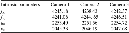
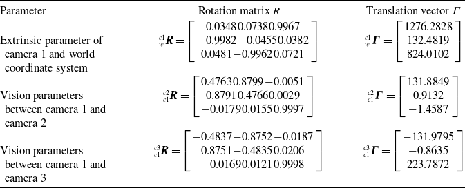
The resulting calibration parameters are presented in Tables 1 and 2.
Intrinsic parameters of multi-cameras detection system

Extrinsic and vision parameters of multi-parameters

The camera 1 captures photos of the calibration board.

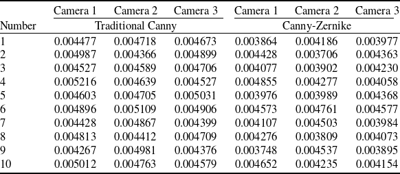
A total of 10 groups of comparative experiments were conducted. In each group, calibration board images corresponding to nine poses were acquired. For the same image, the Canny-Zernike operator and the traditional Canny operator were employed to extract the edges of marker points, followed by camera calibration. The average reprojection errors of the three cameras are presented in the following table (Table 3).
Average reprojection error of the multi-cameras detection system (mm)

Comparison of fitting effects. (a) Canny is applied to calibration board 1. (b) Canny-Zernike is applied to calibration board 1. (c) Canny is applied to calibration board 5. (d) Canny-Zernike is applied to calibration board 5.

It can be seen from the comparison that after extracting the edges of marker points using the Canny-Zernike operator, the average reprojection error of camera 1 is reduced by 9.88%, that of camera 2 by 11.12% and that of camera 3 by 10.95%. Meanwhile, the coefficient of variation (CV, measuring error dispersion) decreases for camera 2 (from 3.14% to 2.58%) and camera 3 (from 4.90% to 4.87%), indicating more stable error distribution. Even for camera 1 with a slightly increased CV, errors concentrate in a lower range owing to the reduced average error. Thus, both calibration accuracy and robustness are significantly improved compared with the traditional Canny operator.
To validate the effectiveness and practicality of the calibration method presented in this paper, a wing-fuselage docking assembly deviation detection system for simulated experiments is constructed, as shown in Fig. 12, which includes a wing-fuselage mating experimental platform and a multi-cameras detection system.
The platform construction of the fork-ear docking assembly deviation detection system.

Utilising the aforementioned system, the wing posture adjustment time is set to 60 s. Firstly, 30 wing-fuselage docking assembly experiments are completed without multi-cameras calibration. Then, Zhang’s calibration method is used to calibrate the multi-cameras to complete 30 wing-fuselage docking assembly experiments. Subsequently, the calibration method in this paper is used to calibrate the multi-cameras and complete 30 wing-fuselage alignment experiments.
Firstly, multi-cameras capture pictures of the initial position of the fuselage-wing. The initial coordinates of the fuselage fork joint hole centre
 ${p_{cf}}\left( {{x_{cf{\rm{i}}}},{y_{cfi}},{z_{cfi}},1} \right)$
and wing ear joint hole centre
 ${p_{cw}}\left( {{x_{cwi}},{y_{cwi}},{z_{cwi}},1} \right)$
in the camera 1 coordinate system are measured by the camera calibration parameters. The position of the fuselage-wing before docking assembly is shown in Fig. 13, and the initial position detection result as shown in Fig. 14.
Position of fuselage-wing fork-ear before assembly.

The fork-ear hole centre coordinate before assembly.

Then, the positioner driving amounts are determined by attitude adjustment calculations. The assembly retention is set to be 9.95 mm in the docking direction and 2 mm in the vertical direction. The coaxiality between the current fuselage fork joint hole centre coordinates and the wing ear joint hole centre coordinates were measured. The coaxiality of the fork-ear during wing-fuselage docking assembly as shown in Fig. 15.
Fork-ears coaxiality error during the assembly. (a) Fork-ear 1 coaxiality error. (b) Fork-ear 2 coaxiality error.

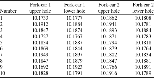
The theoretical coaxiality in the current wing-fuselage docking assembly process is 10.1490 mm. Taking into account the repeat positioning error of the positioners, the actual coaxiality will vary. The measured coaxiality is presented in Table 4.
Fork-ears1and 2 coaxiality error during assembly (mm)

The position is fine-tuned by measurement results to assemble the wing-fuselage. The pre-assembly position and results after assembly are shown in Fig. 16. As shown in the figure, the docking assembly results are in line with the expected results.
Pre-assembly position and results after assembly. (a) Fork-ear position before assembly. (b) Fork-ear position after assembly.

Finally, we have obtained the errors between the four-hole centre coordinates of the two wing ear joints and their respective theoretical coordinates, and then derived the average error of the hole centre coordinates for these ear joints from these errors. The calibration effect of the proposed method is verified by comparing the detection results of the fork-ear position deviation after the wing-fuselage docking assembly experiments are completed in three cases. Fork-ear hole centre X, Y, Z direction errors are shown in Fig. 17.
Fork-ear hole centre X, Y, Z direction error. (a) The range of the average error in the X-direction of the fork-ear hole centre. (b) The range of the average error in the Y-direction of the fork-ear hole centre. (c) The range of the average error in the Z-direction of the fork-ear hole centre.

The coordinates of the wing attitude adjustment control points are measured by the laser tracker, and the wing pose error is obtained by comparing the theoretical position mathematical model of the wing, as shown in Fig. 18.
Results comparison of fork-ear posture deviation detection. (a) Deviation range comparison of
 ${x_g}$
-axis. (b) Deviation range comparison of
 ${y_g}$
-axis. (c) Deviation range comparison of
 ${z_g}$
-axis. (d) Deviation range comparison of roll angle
 $\varphi $
. (e) Deviation range comparison of roll angle
 $\theta $
. (f) Deviation range comparison of yawing angle
 $\psi $
.

The analysis shows that without calibration, the deviation range of fork-ear docking positions is −0.064 mm to 0.069 mm, and the deviation range of attitude angle is −0.1845° to 0.1815°. When using Zhang’s calibration method, the deviation range of fork-ear docking positions is −0.052 mm to 0.053 mm, and the deviation range of attitude angle is −0.1466° to 0.1484°. When using the proposed calibration method in this paper, the deviation range of fork-ear docking positions is −0.043 mm to 0.045 mm, and the deviation range of attitude angle is −0.1185° to 0.1179°. According to the experimental results, after the completion of the wing-fuselage docking assembly, the lower deviation of the wing position range has been reduced from −0.064 mm to −0.043 mm, while the upper deviation has been reduced from 0.069 mm to 0.045 mm. For the wing attitude angle deviation range, the lower deviation has decreased from −0.1845° to −0.1185°, and the upper deviation from 0.1815° to 0.1179°. These results demonstrate that the multi-cameras calibration method proposed in this paper can effectively enhance the calibration and detection accuracy of multi-cameras systems, thereby improving the assembly quality of large aircraft components.
7.0 Discussion
In this paper, a multi-cameras stereo calibration method is proposed for wing-fuselage docking assembly. Based on the Canny-Zernike sub-pixel edge detection method, the high-precision circular edge and centre are obtained. At the same time, the stereo calibration is realised by combining Zhang Zhengyou calibration method, Levenberg-Marquardt distortion correction algorithm and coordinate transformation principle. This section will discuss the research results, existing limitations, and the industrial application of the model.
-
(1) In the docking experiment, the Canny-Zernike sub-pixel edge detection method is used to fit the edge of the fork-ear hole, and the fitting effect is good. The position relationship between the cameras is obtained by Equations (36) and (37), and the sub-pixel edge detection fitting result of Canny-Zernike is introduced to solve the coordinates of the centre point of the fork-ear hole under camera 1. The detection accuracy is further improved compared with Zhang’s calibration method, and the wing-fuselage docking assembly accuracy is further improved compared with the docking method using Zhang’s calibration method.
-
(2) The limitations of the calibration method proposed in this paper mainly stem from two core aspects, with additional inherent constraints requiring critical reflection – these are closely tied to hardware dependence, environmental adaptability and algorithmic stability, and are elaborated as follows:
-
(a) Under complex working conditions, limited by the size and layout of assembly equipment, the field of view and installation position of visual measurement equipment may be restricted, which directly reduces the coverage of effective calibration areas. For instance, in the docking of ultra-large aircraft components (e.g., wing spars or fuselage sections), the fixed layout of multi-camerass often fails to fully capture the calibration board features in narrow gaps between components, leading to incomplete data acquisition.
-
(b) In specific assembly scenarios, occlusion by docking assembly equipment can result in insufficient brightness of the calibration board, degrading calibration accuracy. Meanwhile, fluctuations in temperature and humidity can cause minor deformations of the calibration board or changes in camera lens parameters, further introducing errors into calibration results.
Beyond the above, three more critical limitations need emphasis:
-
(c) The method essentially relies on the physical features of the calibration board (a 7 × 7 array of solid circles markers), leading to hardware-algorithm coupling. For the docking of large aircraft components, the existing 150 mm × 150 mm calibration board has insufficient measurement coverage, necessitating the customisation of oversized calibration boards.
-
(d) Although the Canny-Zernike sub-pixel edge detection outperforms traditional algorithms in noise resistance, its performance degrades in outdoor temporary assembly scenarios. Under strong backlighting or dusty environments, the edge extraction error will still increase significantly – and this method has not been validated in outdoor scenarios, leaving a gap in its practical applicability for off-site operations.
-
(e) The iterative convergence of the Levenberg-Marquardt distortion correction algorithm depends heavily on initial parameters. If the initial values deviate significantly, the algorithm may converge to local optimal solutions rather than the global optimum, undermining calibration accuracy.
-
-
(3) With regard to the potential industrial application of the model, the following two scenarios are worth discussing:
-
(a) The model proposed in this paper can be used for aircraft large parts assembly. The position deviation of the fork-ear during the assembly of large parts of the aircraft may lead to joint collision or out of tolerance during docking assembly. Therefore, the calibration method proposed in this paper can improve the accuracy of docking assembly and prevent joint collision or out of tolerance.
-
(b) In aircraft cabin docking or missile silo docking, the calibration method proposed in this paper can accurately measure the centre of the end pin hole or the coordinates of the feature points, improve the accuracy of the cabin pose measurement and improve the quality of the cabin-end docking assembly.
-
8.0 Conclusion
-
(1) A multi-cameras calibration method for large aircraft component docking assembly is proposed. The Canny-Zernike algorithm is proposed to extract the features of the solid circle on the calibration board. A circle centre sorting method based on triangle marker is introduced to achieve the sorting of the circle centre. The intrinsic and extrinsic parameters of each camera were solved separately using Zhang’s calibration method, while the visual parameters among the three cameras were obtained using the indirect calibration method. The Levenberg-Marquardt algorithm is used to optimise the distortion correction model.
-
(2) The results demonstrate that the proposed multi-cameras calibration method for large aircraft component docking assembly achieves stereo calibration of the multi-cameras under complex working conditions and enhances the calibration accuracy. Compared to the uncalibrated state and the use of Zhang’s calibration method, the accuracy of the deviation detection range is enhanced to −0.043 mm to 0.045 mm, and the accuracy of the attitude angle deviation detection range is enhanced to −0.1185° to 0.1179°.
-
(3) This method is not only suitable for the docking assembly of large aircraft components but also suitable for aerospace and other complex structural products. It has important theoretical significance and practical engineering value for improving the accuracy of calibration and detection, reducing the development cost and improving the quality of large component docking assembly.
Author contributions
Conceptualisation, Xingyuan Tian and Du Li; data curation, Xingyuan Tian; formal analysis, Xingyuan Tian; funding acquisition, Yongguo Zhu and Bingduo Hou; investigation, Yongguo Zhu; methodology, Weipeng Jiang; project administration, Yongguo Zhu ; resources, Yongguo Zhu; supervision, Bingduo Hou; validation, Du Li and Weipeng Jiang; writing – original draft, Du Li; writing – review & editing, Xingyuan Tian. All authors have read and agreed to the published version of the paper.
Financial support
Funding: This research was funded by the Jiangxi Provincial Key Research and Development Plan (No. 20243BBG71004), the National Natural Science Foundation of China (No. 52465060), and the Aeronautical Science Foundation of China (No. 2024M050056002).
Data availability statement
Data are contained within the article.
Acknowledgments
The authors acknowledge the equipment support provided by the Jiangxi Provincial Key Laboratory of Digital Assembly, Nanchang Hangkong University.
Competing interests
The authors declare no conflicts of interest.