1. Introduction

Social exchanges often involve a time lag between promise and delivery. This is not just common to market exchanges, but to political exchanges as well. Markets often involve anonymous, one-shot transactions, and the working of democracies presupposes that when a citizen gives her vote she expects the representative to fulfill his part of an informal, tacit ‘contract.’ Both sides can benefit from an honest exchange, yet there is the potential for cheating. The motivations of those we interact with cannot be known directly, and the quality of goods and services we are offered is often unknown. If we trust, we make ourselves vulnerable to exploitation, since others’ behavior is not under our control. By trust we thus mean a disposition to engage in social exchanges that involve uncertainty and vulnerability, but that are also potentially rewarding. This disposition may be grounded upon a belief in the trustworthiness of the specific agents with whom we interact, either because we directly or indirectly know about their past behavior, or else because we see that it might be in their long-term interest to reward our trust, even if their short-term interests militate against rewarding it. The most interesting cases, however, are those in which it may not be in another's self-interest (however defined) to be trustworthy, we do not have personal experience with this person, group or organization, but entering into a relation (commercial, political, etc.) with it may prove extremely profitable. In situations in which we have little information and little time to gather more, trust might be better described as a disposition to engage in impersonal social exchanges, hence the name ‘impersonal trust.’ People may of course have expectations of trustworthiness also in these situations, but these expectations will not be grounded upon the recognition that it is in the other party's interest to be perceived as trustworthy.Footnote ¹ Expectations in this case may be adaptive, meaning that past experiences will loom large in one's willingness to trust and/or reciprocate in impersonal, even anonymous exchanges. What we are modeling here, however, is not the emergence of expectations about the trustworthiness of other parties or institutions. We are rather interested in the emergence of a behavioral pattern of trusting/reciprocating.

Note that the problem of impersonal trust is a classical case of a one-sided social dilemma.Footnote ² The standard solution to “social dilemmas” is to introduce some form of formal or informal social control. Formal controls involve the existence of ‘impartial’ agencies that monitor and sanction compliance with agreements we enter into. Institutional protection, however, can be costly. Monitoring and sanctioning require a complex organization, and often the very existence of such formal controls can be counterproductive (Fehr, Gachter, and Kirchsteiger Reference Fehr, Gachter and Kirchsteiger1997), in that it creates an atmosphere of distrust. Informal controls instead rest on the possibility of repeated, non-anonymous interactions. The repetition itself, with its possibilities for signaling, retaliation, and reputation formation, becomes an enforcement mechanism. Thus a network of stable exchange relationships is a source of trust, since people will prefer to transact with individuals or organizations that have a known reputation for honesty. The drawback of this solution is that transactions will be limited to a restricted network. Patron-client political exchanges, as well as the common business practice of shunning better deals in favor of established suppliers (Yamagishi and Yamagishi Reference Yamagishi and Yamagishi1994) are examples of parochial tendencies that may ultimately backfire, if the opportunity cost of avoiding the open market becomes too great. The problem of how impersonal trust can emerge and persist is thus intertwined with the possibility of the transient and anonymous social exchanges that are the foundation of market economies and democratic systems.Footnote ³ When there is an occasion for cheating, there is often the promise of great gain, and though the incidence of dishonesty may be higher among strangers than among neighbors, it is by no means a universal phenomenon.Footnote ⁴

Our goal is to model how a behavioral pattern of trusting and reciprocating may develop among boundedly rational agents in a complex environment in the absence of formal or informal controls.Footnote ⁵ To do that, we abandon the traditional assumptions of perfect rationality, unlimited calculating capabilities, and extensive knowledge that are the backbone of classical game-theoretic models. In the complex environments we consider, computing an optimal strategy is a daunting task. What we instead model is the process through which different strategies interact and how their mix evolves. In an evolutionary model, strategies that have been relatively effective in a population become more widespread, and strategies that have been less effective become less common in the population. There is by now a vast literature on the evolution of cooperative strategies in Prisoner's dilemma games (Axelrod Reference Axelrod1984). The kind of interaction we study is called a Trust game, and is like an alternating, one-sided Prisoner's dilemma, in that players have asymmetric roles and move sequentially, and only one of them is given the chance of cooperating or defecting at any time. Another difference between our model and those that study the emergence of cooperation in evolutionary games is that in our model strategies are not just history-contingent; they are also role-contingent, in the sense that a player must have a plan of action for each of the roles (truster or trustee) in which she may be cast.

The paper shows the results of deterministic and stochastic simulations in both one-shot and repeated versions of the Trust game. The present results show how trust and reciprocity can emerge in a population of strangers and examine whether these behaviors remain robust to a change in the size of the strategy space and/or the length of the game. An interesting result of both simulations is that many of the conditional pure strategies support trusting/reciprocating or ‘cooperative’ behavior, but none of them is an evolutionarily stable strategy. In fact, the concept of evolutionarily stable strategy is not the relevant analytic concept here. The relevant analytic concept here is that of an evolutionarily stable state, which means a stable mix of strategies appearing in different proportions in the population.Footnote ⁶ What we have is a vector of strategies, or a polymorphic population, in which each player uses a pure strategy and different players may use different strategies. These populations are made of a stable majority of conditional trusting/reciprocating types; interestingly, unconditional trusting/reciprocating types can survive as a small minority only in those populations where the majority is made of conditional types.

In our model, though the underlying strategies are heterogeneous, observable actions are homogenous, i.e., trusting/reciprocating behavior is widespread. This means that an external observer would detect a behavioral regularity, and might be misled into thinking that players use the same strategy, possibly an unconditional one. A social norm is, among other things, a regular behavioral pattern. The behavior dictated by a norm, however, is usually conditional.Footnote ⁷ Indeed, an important difference between a social norm and an unconditional rule or imperative is precisely the fact that a social norm is conditional. An unconditional imperative might tell us to “trust, no matter what,” or “always reciprocate.” A social norm instead tells us to trust/reciprocate under various conditions, and to stop trusting/reciprocating if these conditions are not met. In this sense we may think of a norm as subsuming several different strategies that produce the same behavior under the right circumstances. Even more important, we show that the same social norm may be supported by different types of strategy combinations, where the exact polymorphism will depend upon the initial set of basic strategies.

As Brian Skyrms (Reference Skyrms1996, Reference Skyrms, Bicchieri, Jeffrey and Skyrms1997) has repeatedly argued, a crucial element in the study of norms is an analysis of their emergence. Only a dynamic model allows us to see the history of the emergence of a norm, and the reasons for its change or persistence. In our case, the dynamics are driven by payoff-relevant information, and the use of a simulation lets us see what happens along the path, or how strategies evolve over time. There are advantages to using simulations instead of calculating the limit of the process using a set of difference equations.Footnote ⁸ A simulation eases the process of testing alternative hypotheses that is crucial for understanding how and why different strategies, in different proportions, may converge to a fixed point, or an invariant distribution of strategies. In addition, stochastic difference equation systems are notoriously hard to analyze and the difficulty is compounded—in the case of our model—by the existence of a large strategy space.

It is important to notice that the results obtained in our deterministic simulation are confirmed in the stochastic one. In the latter simulation, the dependence on initial conditions (the initial population proportions) is removed; hence the stable long-run equilibria we observe are a function of the length of the iterated game and the given strategy mix only. In both kinds of simulations, the final stable mix of conditionally cooperative strategies will depend upon the strategies that are currently being played.Footnote ⁹ However, even in environments in which more diverse and complex conditional strategies are present, the final result will be a mix of conditionally cooperative strategies, and unconditional noncooperators will tend to die out, whereas unconditional cooperators will find a niche within the population. We may conclude that, in the long run, norms of trust and reciprocity tend to emerge, provided the initial population contains some conditionally cooperative strategies, irrespective of the specific methods used by these strategies to elicit reciprocity and punish transgressions.Footnote ¹⁰

2. The Trust Game

In an interaction, a player can be either in the role of the truster (sender), or in the role of the trustee (receiver). To model the fact that a player has no control over which role he will be cast in, we use an extensive form game (Figure 1) in which Nature moves first. With probability p, Nature assigns to player i the role of sender and to player j the role of receiver, and the reverse with probability (1−p). This game is a version of the ‘investment’ or ‘trust’ game studied by Kreps (Reference Kreps, Alt and Shepsle1990), Bicchieri (Reference Bicchieri1993), and Berg et al. (Reference Berg, Dickhaut and McCabe1995). After the players’ roles have been assigned, the sender moves first and must decide whether or not to ‘trust’ the receiver with her endowment of x dollars. If the sender chooses to trust (invest), the size of her endowment is tripled to 3x, and the receiver must then decide whether to reciprocate, returning 3x/2 to the sender and keeping 3x/2 for himself, or to not reciprocate and keep all 3x for himself. The action set for the sender is to trust or not to trust, a = {T, nT}, and the action set for the receiver is to reciprocate or not reciprocate, b = {R, nR}.

Figure 1.

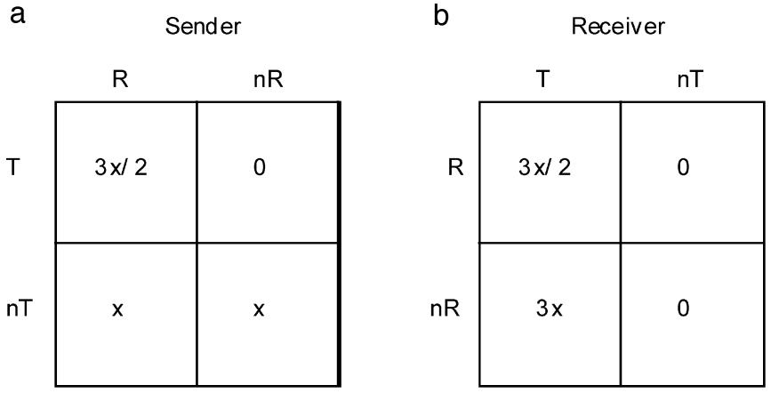
Once a role has been assigned, each player faces a simple 2x2-payoff matrix, depicted in Figures 2a and 2b. In Figure 2a, the sender is the row player, and clearly has no dominant strategy. In Figure 2b the receiver is the row player, and he has a weakly dominant strategy: nR.

Figures 2a and 2b.

Players, however, have to choose a strategy before knowing which role they will be assigned by nature. In the simplest case, which we examine first, each player has four strategies to choose from: {TR, TnR, nTR, nTnR}. Let us call this set of strategies the minimal strategy space. These strategies are role-contingent, in that they dictate how the player should play the game when he finds himself in each role:

1. TR: when in the sender position, always trust. When in the receiver position, always reciprocate.

2. TnR: trust as sender, do not reciprocate as receiver.

3. nTR: do not trust as sender, but always reciprocate as receiver

4. nTnR: when sender, do not trust. When receiver, do not reciprocate.

Notice that these strategies, while role-contingent, are not conditional on a player's past history of play. In this sense, this set of strategies may be regarded as unconditional, but role-contingent imperatives. For example, TR may be interpreted as the imperative of being unconditionally cooperative, no matter what. Later on we will enlarge the strategy space to include both the minimal strategy space as well as strategies that are conditional on a player's past history of play.

In the remainder of the paper, we shall assume for simplicity that the probability of being cast in either role (sender/receiver) is $p=1/ 2$ ; this will allow us to construct a single, symmetric payoff matrix for the trust game. In the game of Figure 1, then, each player is facing the following 4x4 payoff matrix (Figure 3), which takes the weighted average of playing sender or receiver with probability 1/2. As in Figure 2b, where nR weakly dominated R, here nTnR weakly dominates nTR, and TnR weakly dominates TR.

Figure 3.

In what follows we consider a sequence $g=1,2$ ,…, n, of both one-shot (OS) and repeated (R) games represented by a symmetric payoff matrix A, such as that given in Figure 3. In OS games, the game number g, and round number $t=1,2$, …will be synonymous, while in R games, the round number t will start anew, $t=1,2$, …for each new R, “supergame” number g. The main difference between the two environments is in the realization of payoffs; in the OS game, payoffs are realized after a single round, whereas in the R game, the sum of payoffs from all rounds played is realized at the end of each supergame, consisting of a sequence of rounds.

In both environments, each player plays a single pure strategy from the given set of strategies in all rounds of a game. As explained in further detail below, the payoff to using a particular strategy does not depend on the strategy adopted by a player's opponent or sequence of opponents. Rather, we consider how each strategy fares against the population of strategies as a whole—what Maynard Smith calls “playing the field.”Footnote ¹¹

If $g\leq n,$ then following the completion of each OS or R game, the fitness of each strategy is evaluated. The fitness of a strategy in the OS game is its weighted average payoff against the population of strategies in the one-round game. The fitness of a strategy in the R game is its weighted average payoff against the population in all rounds of the R game. These fitness values are used to adjust the proportion of the population that is playing each of the pure strategies in the subsequent OS or R game, as explained in further detail below. In the repeated game, we imagine that players discount future earnings by the factor 1-δ per round, where δ ∊ (0, 1) can be interpreted as the constant probability that the game ends from one round to the next. Thus, the mean number of rounds in each of the n repeated games is $r=1/ \delta $ .Footnote ¹²

3. Equilibria in OS or R Games

In the OS game, the unique subgame perfect Nash equilibrium is for receivers to play nR, and therefore for senders to play nT, i.e., in the symmetric game, all players play the strategy nTnR. In the repeated game, it is possible for players to cooperate with each other, and thus do better. Indeed, the folk theorem for repeated games states that, for a low enough discounting of future payoffs, there are many equilibria in which the players behave cooperatively towards each other (Fudenberg and Maskin Reference Fudenberg and Maskin1986). For example, a trusting-reciprocating behavioral pattern can be supported as an equilibrium if pairs of players adopt a “grim-trigger” strategy. Suppose a player in the role of sender initially plays T, and keeps playing T if the receiver plays R, but after the first defection (nR), she switches to nT forever. Similarly, the player in the role of the receiver responds with R to T, but if nT is played once, he plays nR forever after. This grim-trigger strategy can be supported as an equilibrium as long as $\delta \leq 1/ 2$ .Footnote ¹³ Other trigger strategies can be used to support a cooperative, trust/reciprocate equilibrium under similar restrictions on δ. These cooperative equilibria exist also in the population game environment that we examine, where players’ strategies are judged by how well they fare against the population of strategies (against the field). In the latter case, the initial proportions of the various strategies in the population may also be a factor (in addition to δ) in whether trust and reciprocity can be sustained (as is shown in our simulations, discussed below).

In sum, as traditional game theory predicts, if players are rational, trust and reciprocity are not sustainable in the one-shot game. However, trust and reciprocity can emerge as stable behaviors when interaction is repeated if players do not discount their future earnings too much, or if they believe with a high enough probability that they are going to meet again.

There are several drawbacks to traditional game-theoretic models. For one, in the repeated game there can be multiple equilibria, and no way to predict which one will occur. To play a particular cooperative equilibrium, players must have common priors about all the possible strategies each of them may use, and this fact must be common knowledge. Thus traditional game-theoretic models impose rather heavy informational and computational requirements upon the players.

Furthermore, rationality alone cannot explain how players learn to play a Nash equilibrium, nor can rationality arguments be used to select from among multiple equilibria.Footnote ¹⁴ Researchers have therefore turned to bounded rationality approaches to model the adoption and selection of Nash equilibria. Bounded rationality approaches in game theory can be divided into two types, depending on whether the focus is on individual behavior or on population dynamics instead. Individual learning theories, for example, assume some exogenous process for matching players, and describe the manner by which individual players update their beliefs, e.g., the “fictitious play” learning model (see, e.g., Skyrms Reference Skyrms1990). Individuals are assumed to play best responses to their most recent beliefs. By contrast, evolutionary theories are inspired by population biology (e.g., Maynard Smith and Price Reference Maynard Smith and Price1973). These theories dispense with the notion of the individual, as well as with best responses/optimization, and use in their place a natural selection, ‘survival-of-the-fittest’ process together with mutations to model the frequencies with which various strategies are represented in the population over time. We have chosen to pursue an evolutionary learning approach using computer simulations to obtain our main findings.

In the following simulations, players are identified with a strategy, and the relative frequency of a strategy in a population is simply the proportion of players in that population who adopt it. The relative frequency of each strategy in the population at round t is a function of its payoff relative to the population average. In our deterministic evolutionary model, inferior strategies die out, but it is difficult to keep this interpretation whenever a player is identified with a strategy.Footnote ¹⁵ Players do not necessarily die out. Instead we can suppose that they may simply change their strategies. Thus a more complete model of how a trusting/reciprocating behavioral pattern could emerge as the dominant one would include a description of how adaptive players change their strategies on the basis of previous outcomes.

The main solution concept used in evolutionary game theory is the evolutionarily stable strategy (ESS) introduced by Maynard Smith and Price (Reference Maynard Smith and Price1973), or the evolutionarily stable state (ESSt) for population-wide frequencies of strategies (see, e.g., Hofbauer and Sigmund Reference Hofbauer and Sigmund1998).

Since we are examining behavior in a population game in which each player plays a pure strategy, we shall adopt the latter concept.Footnote ¹⁶ Suppose there are N pure strategies for the trust game, with an NxN symmetric payoff matrix $\mathrm{A}\,=\left(\mathrm{a}\,_{\mathrm{ij}\,}\right)$ (Figure 3 gives A for the case where $N=4$ ). Each member of the continuum of players initially commits to playing exactly one of the N pure strategies (we do not allow mixtures). Let p be the $N\times 1$ vector denoting the population-wide proportion of each of the N strategies (player types) in the population. Let

denote the fitness of strategy i. The population-wide weighted xaverage fitness value is $p^{T}Ap$. We say that $\hat{p}$ is an evolutionarily stable state (ESSt) if, for any p

And if $p\neq \hat{p}$ and$p^{T}A\hat{p}=\hat{p}^{T}A\hat{p}$ , then

The first inequality is just the definition of a Nash equilibrium. The second inequality is a further refinement that guarantees that $\hat{p}$ is not invadable; that is, $\hat{p}$ fares better against p than p fares against itself.

The definition of an ESSt does not refer to a specific dynamic, but biologists and evolutionary game theorists frequently use a replicator dynamic, which in its deterministic form can be written as:

where p(t) denotes the population-wide proportion as of time t. Hence, strategies with above average fitness see their proportions increase, and those with below average fitness see their proportions decrease.Footnote ¹⁷

It is well known that (ESSt) are asymptotically stable fixed points of this replicator dynamic, though the converse of this statement need not be true (see, e.g., Samuelson Reference Samuelson1997).Footnote ¹⁸ A similar relationship holds between the replicator dynamic and Nash equilibria: if $\hat{p}$ is a Nash equilibrium of the symmetric game A, then $\hat{p}$ is a stationary state of the replicator dynamic.

4. The Evolutionary Model

We use both a deterministic and stochastic discrete-time replicator dynamic to characterize the distribution of strategies in the population over time. The system has an evolutionary flavor in the sense that each strategy's share in the population increases or decreases with increases or decreases in that strategy's payoff performance relative to the population average payoff. Furthermore, in the stochastic version of the model, mutations in the proportions of the various strategies in the population insure that no strategy becomes extinct.Footnote ¹⁹ This simple, dynamical model is based on one used in population biology and was imported into game theory by Foster and Young (Reference Foster and Young1990; Young and Foster Reference Young and Foster1991), who introduced the idea of a stochastically stable equilibrium.

4.2. Stochastic Version

Foster and Young (Reference Foster and Young1990) pointed out that the deterministic system (1) allows some strategies to become extinct, in the sense that $\mathrm{p}\,_{\mathrm{i}\,}(\mathrm{t}\,) =0$ for some i,t. The possibility of extinction runs counter to the (biological) notion that populations are subject to invasion and strategies (species) that are near extinction may thrive once again when environmental conditions change in their favor. Furthermore, there is the possibility of new strategies (species) as well, however we do not consider this possibility here. To prevent extinction, we can add mutation to the model in several ways. For example, we can perturb the payoff matrix A slightly each period as in Fudenberg and Harris Reference Fudenberg and Harris1992, or we can add noise to the deterministic updating of the proportion vector p(t) as in Foster and Young Reference Foster and Young1990, or we can do both. Perturbing the payoff matrix can be interpreted as uncertainty concerning the expected payoffs, while perturbations to the proportion vector can be interpreted as persistent experimentation (or non-extinction).

We propose, as our stochastic model, the latter type of mutation. Specifically, let the proportions now evolve according to:

where $\epsilon _{i}(t+1) $ is a draw from a standard normal distribution, and s is a tuning parameter. The algorithm we used is implemented as follows. In each period, we calculate the proportions according to (2). We then rebalance these proportions, by dividing each $p_{i}(t+1) $ by the sum $\sum_{i=1}^{N}p_{i}(t+1) $ . Our interest is in the evolution of the proportion vector p (t) over time for “small” values of s. Foster and Young showed that the behavior of the stochastic system can be quite different from the behavior of the deterministic system. In particular, the stochastic system removes the possibility of absorbing states at the boundary of the N−1 dimensional simplex that characterizes the distribution of strategies in the population, and under certain conditions, can result in a unique, “stochastically stable” equilibrium proportion vector.

Because we are interested in examining the emergence of a behavioral regularity in a relatively large strategy space (later on we will examine up to 16 strategies), analytic results are difficult to achieve. We therefore make use of numerical simulations as described in the next section.

5. Simulations.Footnote ²⁰

5.1. One-Shot Game

In the one-shot game, A is the 4x4 symmetric matrix depicted in Figure 3. In the simulations, we set $x=1$ , so the actual matrix used is given in Figure 4. All of the simulation experiments reported in this section were conducted using the simple deterministic replicator dynamic (1).Footnote ²¹ The initial proportions of strategies were varied according to what we thought were interesting initial conditions, and the simulations were carried out for a sufficiently large number of periods (1,000 iterations for each initial condition) to insure that the limiting, stationary proportions of the replicator dynamic had obtained. Each round in a simulation corresponds to the play of a single one-shot game. Our results consider the proportion of the various strategies observed in the population at the end of 1,000 iterations.

Figure 4.

The main results can be summarized as follows. First, as long as there is initially some positive proportion of the population playing nR, the proportion of players playing R (either as TR or nTR) will disappear.Footnote ²² If the initial proportion playing nR is zero, then T will come to dominate nT, as long as there is some positive proportion of players initially playing T.

Table 1 shows 27 initial frequencies (conditions) for the basic four strategy version of our game, and what happens to these frequencies following 1000 iterations of the deterministic replicator dynamic. Note that in a simulation where the initial population has any positive proportion of the nTnR strategy, the final result will be a population dominated by nTnR players (but see condition 13 below for an exception). For example, if the initial vector $p=(.25,.25,.25,.25) $ , which corresponds to condition 21 in Table 1, the limiting proportion vector as illustrated in Figure 5 is: .0 TR, .0 TnR, 0.121 nTR and 0.879 nTnR. This is the limiting vector because the boundary is an absorbing state. As Figure 5 illustrates, the convergence in the deterministic case happens after about 10 iterations, so 1000 iterations is plenty.

Table 1.

Initial Condition #	Strategy	Initial Frequency	Final Frequency*
1	TR	1	1
	TnR	0	0
	nTR	0	0
	nTnR	0	0
2	TR	0	0
	TnR	1	1
	nTR	0	0
	nTnR	0	0
3	TR	0	0
	TnR	0	0
	nTR	1	1
	nTnR	0	0
4	TR	0	0
	TnR	0	0
	nTR	0	0
	nTnR	1	1
5	TR	0.99	0
	TnR	0.01	1
	nTR	0	0
	nTnR	0	0
6	TR	0.99	1
	TnR	0	0
	nTR	0.01	0
	nTnR	0	0
7	Tr	0.99	0
	TnR	0	0
	nTR	0	0
	nTnR	0.01	1
8	Tr	0.01	0
	TnR	0.99	1
	nTR	0	0
	nTnR	0	0
9	Tr	0	0
	TnR	0.99	1
	nTR	0.01	0
	nTnR	0	0
10	Tr	0	0
	TnR	0.99	0
	nTR	0	0
	nTnR	0.01	1
11	Tr	0.01	1
	TnR	0	0
	nTR	0.99	0
	nTnR	0	0
12	Tr	0	0
	TnR	0.01	1
	nTR	0.99	0
	nTnR	0	0
13	Tr	0	0
	TnR	0	0
	nTR	0.99	0.99
	nTnR	0.11	0.11
14	Tr	0.01	0
	TnR	0	0
	nTR	0	0
	nTnR	0.99	1
15	Tr	0	0
	TnR	0.01	0
	nTR	0	0
	nTnR	0.99	1
16	Tr	0	0
	TnR	0	0
	nTR	0.01	0.01
	nTnR	0.99	0.99
17	Tr	0.97	0
	TnR	0.01	0
	nTR	0.01	0.000577428
	nTnR	0.01	0.999423
18	Tr	0.01	0
	TnR	0.97	0
	nTR	0.01	0.000577428
	nTnR	0.01	0.999423
19	Tr	0.01	0
	TnR	0.01	0
	nTR	0.97	0.0673118
	nTnR	0.01	0.932688
20	Tr	0.01	0
	TnR	0.01	0
	nTR	0.01	0.00989659
	nTnR	0.97	0.990103
21	Tr	0.25	0
	TnR	0.25	0
	nTR	0.25	0.121004
	nTnR	0.25	0.878996
22	Tr	0.25	0
	TnR	0.25	0
	nTR	0.01	0.00666536
	nTnR	0.49	0.993335
23	Tr	0.25	0
	TnR	0.25	0
	nTR	0.49	0.0303428
	nTnR	0.01	0.969657
24	Tr	0.5	1
	TnR	0	0
	nTR	0.5	0
	nTnR	0	0
25	Tr	0.48	0
	TnR	0.02	1
	nTR	0.48	0
	nTnR	0	0
26	Tr	0.48	0
	TnR	0	0
	nTR	0	0
	nTnR	0.48	0.0482243
27	Tr	0.48	0
	TnR	0.01	0
	nTR	0.48	0.0307279
	nTnR	0.01	0.969272

Figure 5.

Similarly, if the initial population is composed only of nTR players and nTnR players, then both strategies will survive, because if no players trust, then the receiver's strategy does not matter. For example, if $p(0) =(.0,.0,.99,.01) $ , as in condition 13 of Table 1, the system does not move away at all from this initial condition, where we have .99 nTR and .01 nTnR. This can happen because, if almost everyone is playing nTR, there is never an opportunity for nR to spread, as receivers never get to make any choice. In general, many initial conditions will end up on the boundary between nTR and nTnR, though far closer to nTnR. These anomalous results disappear once we add a stochastic element to the population updating procedure.

The conclusion of our simulation exercise for the one-shot game is that we get stable polymorphic equilibria. However, any population vector composed entirely of non-trusting strategies will not change over time, hence we may consider this vector an evolutionarily stable state.

5.2. Repeated Game

In the repeated game setting, each game consists of a number of rounds, r. In each round, each player type (defined by its strategy) plays its strategy against all player types (including itself) according to their proportions in the population, yielding a certain population-weighted payoff for each strategy for each round. The strategy proportions do not change until the end of the r-rounds. At the end of each repeated game, the proportions of the various types of players are updated according to the replicator dynamic given in equation (1), where the fitness of strategy i is based on its performance over all r rounds of the game.

Recall that the value of $r=1/ \delta $ , where δ can be interpreted as the constant probability that the game ends from one round to the next (alternatively, 1−δ is the constant discount factor for payoffs). Thus, r increases as δ decreases. In all our repeated game simulations, we varied δ from 1 to .0333, so that r varied from 1 (one-shot game) to 30 rounds of play.Footnote ²³

In the repeated game setting we introduce conditional strategies, since repetition allows for more complex behavior. In what follows, we consider a minimum number of conditional strategies to better understand their individual contribution to the establishment of a cooperative behavioral pattern. There are four sending and four receiving strategies:

Sender

1. 1. Always trust (T).

2. 2. Never trust (nT).

3. 3. Grim trigger (G)– Trust until you are not reciprocated and then do not trust for the rest of the interaction.

4. 4. Hopeful (H)– Trust, and then if you are not reciprocated, retaliate by not trusting in the next round. The round after that, trust again, as a sign of your willingness to trust. If you are still not reciprocated, do not trust for the rest of the interaction. If you are reciprocated, return to the beginning of this strategy.

The Hopeful strategy is one of many possible retaliatory strategies. When playing Hopeful, a player stops signaling her willingness to trust after she gets a non-reciprocating response for two rounds, but one can build other strategies in which a player keeps signaling her willingness to trust in the face of several defections. In fact, one could make “hopefulness” a function of the stopping probability, i.e., the lower the probability the game will end soon, the more likely it is that a player “tries again” to signal her willingness to trust. As we explain in footnote Footnote 25, we tried other, more complicated ‘hopeful’ strategies that employ more rounds of punishment. However, we found that these alternative strategies always did marginally worse that the standard Hopeful one.

Receiver

1. 1. Always reciprocate (R).

2. 2. Never reciprocate (nR).

3. 3. Grim trigger (G)–Reciprocate until you are not trusted, then do not reciprocate for the rest of the interaction.

4. 4. Selfish (S)–Start by not reciprocating if you are trusted. If you are not trusted in one round, switch to reciprocating in future rounds in which you are trusted.Footnote ²⁴

The Selfish strategy is one in which the receiver “tests” the sender. If the sender retaliates, the receiver switches to cooperative behavior.

Given the four sender and receiver strategies, there are 16 possible combinations of strategies for players in the repeated game. These are: TR, TnR, TG, TS, nTR, nTnR, nTG, nTS, GR, GnR, GG, GS, HR, HnR, HG, and HS. Figures 6a and 6b represent, respectively, the 4x4 payoff matrices for sender and receiver. Each element of the matrix is the cumulative payoff obtained at the end of r rounds of play between the column strategy and the row strategy. These matrices are expanded into 16x16 matrices, as before, and then averaged to represent the equal probability of being cast in the role of sender or receiver. Some payoffs have been expressed as piecewise functions. For example, in the sender's matrix, we have that, HnR (1) = 0, HnR (2) = 1, HnR (x) = x–2, HS (1) = 0, and HS (x) = 1.5x–2. In the receiver's matrix, the values would be nRH (1) = 3, nRH (2) = 3, nRH (x) = 6, SH (1) = 3, and SH (x) = 1.5x.

Figures 6a and 6b.

We use the same deterministic replicator dynamic (1) as before. However, the payoff matrix A is now the larger 16x16 payoff matrix.Footnote ²⁵ In the simulation exercises reported below, we varied r, the number of rounds played (equivalently, the inverse of the discount factor) from 1 to 30. We also experimented with different initial proportions of strategies in the population. For each set of initial proportions and value of r, we simulated the deterministic replicator dynamic for a sufficiently long time (1000 periods) to ensure that the limiting stationary proportions obtained.

6. Results

6.1. The Deterministic Model

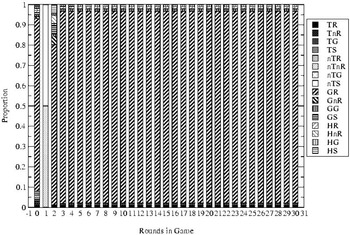
The results of our simulation exercises involving the deterministic replicator dynamic in the repeated game setting depend on the value of r and the initial proportions of strategies in the population. These results can be summarized as follows. In the case where there are equal initial proportions of the 16 strategies, the long-run outcome is a function of the discount factor, or the number of rounds played in each interaction, r (see Figure 7). On the horizontal axis of Figure 7 (and subsequent figures) is the number of rounds per game. The strategy proportions, represented as bars, are average proportions over 1,000 simulated games, always starting with the same initial condition (equal proportions) but different game lengths. It is interesting to note that several contingent strategies support cooperative behavior, but none of them is an ESS.

Figure 7.

Notice that when r = 1, regardless of the initial population proportions, the long-run outcome is mainly composed of nTnR and nTS in equal proportions, with a small number of players playing nTR and nTG. Exceptions occur when nTnR initially dominates the population, as Figure 10 illustrates. In this case, nTnR remains the most prevalent strategy. This result is not too surprising, since when players in our simulation play a one-shot game 1000 times, non-trusting, non-reciprocating strategies dominate as in the simple one-shot game. In short, impersonal trust does not emerge when the length of interactions is short. These conditions are generally true in the case of r = 2 as well, but with a larger proportion of players playing the reciprocating strategies R and G, and fewer playing nR and S.

However, when r = 3, we observe a dramatic shift in favor of players playing GG and GR. It is at this game length that the simple learning strategy embedded in the Grim strategy shows some strength. We also observe a small number of players playing HR and HG. For $\mathrm{r}\,> 3$ , we increasingly observe players playing HR and HG, while the proportion of players playing GG and GR declines. In most cases, the limiting distribution is a mixture of strategies, with about 60% of the players split between HR and HG, 30% split between GR and GG, and 10% playing TR and TG. In short, the only strategies that survive as r grows large are the contingent strategies that favor trust and reciprocation. As the number of rounds increases, a population composed only of these strategies is stable, as all players trust and reciprocate. In addition, a population mainly composed of smart trusters can support a small number of unconditional, “dumb” trusters. It is important to stress that non-contingent strategies such as TR can only survive because of the presence of contingent cooperative strategies.

6.2. Some Exceptions

The results above were for the case of a uniform initial distribution of the 16 strategies in the population. In a population initially dominated by players playing one of the four non-contingent T strategies (TR, TnR, TG, or TS), as r gets large, the long-run outcome is made up of 60% HS and 40% HR/HG. For example, in Figure 8, the population is initially composed of 85% TR and equal proportions of the other 15 strategies. It appears that the reciprocating strategy that gains the most from the existence of a large initial proportion of unconditional trusters is the Selfish strategy. It gains from unconditional trusters by not reciprocating, but learns to reciprocate when faced with players that do retaliate.

A second exception arises when one of the grim or hopeful sender strategies (GR, GG, HR, HG, and HS) makes up a large proportion of the initial population. For example, Figure 9 illustrates the case where 85% of the initial population plays GR, though the same results would hold if any of the other strategies GG, HR, HG, or HS initially dominated to the same degree. In the one-shot, r = 1 game, the result is a distribution of non-trusting strategies. But for $r> 1$ , the dominant initial strategy (GR) remains dominant. When these five strategies are played against each other, HS dominates when r= 1, remains stable when r = 2, and disappears entirely for larger values of r. When nTnR is initially the most frequent strategy, we still observe a shift to the mix of strategies outcome described earlier, but not until r = 10 (see Figure 10, and compare it with Figure 7). nTnR, the fittest strategy in the one-shot game, remains strong for low values of r, but once r equals or exceeds 10, this strategy becomes extinct based on the distribution of results from 1000 r-round games. Notice that in Figures 7–10, it appears as though r= 2 or 3 is usually the indifference point, or tipping point. Before that, non-trusters dominate, and after that, conditional trusters dominate the population.

Figure 8.

Figure 9.

Figure 10.

6.4. Unconditional Strategies

As none of these strategies will perform any differently in a one-shot game as compared to an iterated game, the value of r will not make a difference in the final outcome. Regardless of the initial conditions, we see a convergence (with small fluctuations) to a population vector with mean values: TR = .01, TnR = .01, nTR = .12, nTnR = .86.Footnote ²⁶ An illustration with two different initial proportions is provided in Figures 11a and 11b. These results are qualitatively similar to the deterministic case (compare Figures 11a and 11b to Figure 5). Again, note that we report the average proportions following 1000 games with r-rounds each, where fitness is evaluated at the end of each game. The main difference is the greater volatility in the proportions over time due to the stochastic replicator dynamic. Also, two strategies, TR and TnR are kept from becoming extinct in the stochastic model by the presence of the error term in equation (2)

Figures 11a and b.

6.5. Conditional Strategies

When conditional strategies are considered, for small values of r (i.e., r < 3), the unconditional non-trusters and non-reciprocators dominate the population, as we would expect. However, the results are quite different, as r gets large. Here we report results from an experiment where we add conditional strategies, one at a time, into a population with unconditional strategies. As before, we have removed all dependence on initial conditions, and we observe convergence to a stochastically stable mix of strategies based on the initial mix and on r.Footnote ²⁷ The first case we consider consists of five strategies, the basic four unconditional strategies B4 = {TR, TnR, nTR, nTnR} and the conditional strategy GG. This case is illustrated in Figure 12. For $r> 3$ , the mean proportions (over all r) after 1000 periods are: $\mathrm{TR}\,=.23$ , $\mathrm{TnR}\,=.04$ , $\mathrm{nTR}\,=.04$ , $\mathrm{nTnR}\,=.02$ , GG = .66. The simple addition of a conditional learning Grim/Grim strategy to the mix completely alters the final equilibrium for large r. The GG strategy dominates the population, and the trusting TR strategy is allowed a second place, due to the existence of the conditional GG strategy. The proportions of the other 3 strategies are due to the stochastic replicator dynamic, which prevents these strategies from dying out. We observe a similar finding when we consider the basic four strategies, B4, either combined with GR or with GS. In the latter case, however, we see a new mean proportion mix: TR = .08, TnR = .03, nTR = .50, nTnR = .04, GS = .34. It seems that the selfish strategy, which feeds on unconditional trusters, allows the non-trusting strategy to gain. In addition, the nTR strategy gains from its own unconditional responses to the other trusting strategies in the population.

Figure 12.

Consider next the case where the initial strategies are B4 (the basic four) together with GG and HR. In this case, GG and HR share 66% of the population, but GG does a bit better, most likely due to the absence of the Selfish responding strategy, from which the Hopeful trusting strategy can benefit. However, with B4+GG+GS, GG comes to dominate again and reduces GS to less than 5% of the population. The Selfish strategy only seems to work whenever it is possible to take advantage of unconditional trusters.

The next case to consider is an initial population made up of nTnR, GR, GS, HR, and HS. In this case the final mix of strategies in the population, for large r, is nTnR = .01, GR = .27, GS = .04, HR = .61, HS = .05. We see that the reciprocating strategy does better across the board than the selfish strategy, as most of the conditional trusting strategies end up punishing the selfish strategy. The uncooperative strategy nTnR does not fare well at all.

Finally, we introduced all 16 strategies together in the stochastic model. The result, illustrated in Figure 13a, is a final mix dominated by HR and HG in roughly equal proportions of 20% each. GR/GG come in second place, at about 10% each. Next we see GS/HS at about 6% each. Most other strategies stay around 4–5%, with non-reciprocating strategies doing worse at around 2%, and finally nTnR doing the worst at about 1%. However these last few strategies survive only due to the stochastic nature of the replicator dynamic, which does not let them disappear. In Figure 13b, we observe that this same distribution continues to hold if one of the two the most successful strategies from the previous experiment, HG, dominates the initial population of strategies.

Figure 13a and 13b.

The most important result we obtain is that regardless of the initial population proportions, in the long run we converge to a stationary equilibrium consisting of a polymorphic population of strategies.Footnote ²⁸ Each value of r may result in a different equilibrium outcome but the equilibrium is stable, and is a function only of the initial strategy mix and the value of r, the length of the iterated game. As in the case of the deterministic simulation, as r gets large, conditional strategies come to dominate the population. The unconditional trusting/reciprocating strategies continue to exist, though in small numbers, due to the presence of large numbers of conditionally “nice” strategies. It thus seems that the very existence of a rigid rule that demands unconditional cooperation depends upon the presence of conditionally cooperative practices. As r gets large, non-trusting/non-reciprocating strategies invariably recede to a mere subsistence level. The tuning parameter s represents the weight cast on the stochastic term. Any positive value of s will lead, irrespective of the initial proportions of strategies, to the same equilibrium mix of strategies. For smaller values of s, the system will take more time to converge to an equilibrium mix of strategies, and larger values of s will create more fluctuations in the actual proportions. It will still be the case, however, that the strategies that are dominant in an environment in which there is low variability remain dominant in a high-variability environment.

7. Conclusions

Our goal in this paper was to explicate the development of a social norm of trust and reciprocation. We show that when impersonal trust/reciprocation becomes the dominant observed behavior, it is the outcome of the interaction of several different strategies. It would therefore be a mistake to identify a social norm of trust and reciprocation with a particular strategy, since such a norm is supported by several different strategies. Moreover, such strategies are conditional ones. In fact, many pure strategies support trust/reciprocating behavior, but none of them is an unconditional rule telling a player to trust/reciprocate no matter what. Rather, generalized, impersonal trust only develops as a consequence of the interaction of several conditional strategies that differ in the severity with which they punish transgressions, as well as in their willingness to give other players further chances. Their differences, however, cancel out in our evolutionary model.

For impersonal trust to emerge, interactions between players must go on for extended periods of time. When interactions are only one-shot, players who take what they can and leave do the best. When interactions are repeated, in the presence of conditionally cooperative strategies, anonymous, impersonal trusting/reciprocating behavior can emerge and dominate in this evolutionary model. The resulting stable behavioral pattern (or norm) is thus supported by a polymorphic population of strategies. Regardless of the proportions in which our strategies initially appear in the population, a resulting evolutionarily stable state is reached in which trusting/reciprocating behavior is the norm. Since in our stochastic model no strategy goes extinct, we have a very robust test of a norm's emergence. We hasten to add that, consistent with our interpretation of the results, our conclusions are also conditional. That is, they depend upon the strategy set we have considered. Given our strategy set, there is no unique evolutionarily stable strategy. Rather, we have a polymorphic population of strategies that uphold generalized trust and reciprocation.