Introduction
Deep level transient spectroscopy (DLTS) is a very sensitive method used to measure electrically active deep level traps in semiconductors. DLTS began as a differential capacitive technique developed by Lang in 1974 [Reference Lang1] and has since extended to a variety of other differential charge sensing methods, including charge transient spectroscopy (QTS) [Reference Farmer, Lamp and Meese2], constant capacitance deep level transient spectroscopy (CCDLTS) [Reference Johnson, Bartelink, Gold and Gibbons3], current transient spectroscopy (I-DLTS) [Reference Hurtes, Boulou, Mitonneau and Bois4], and photo-induced current transient spectroscopy (PICTS) [Reference Balland, Zielinger, Tapiero, Gross and Noguet5]. These various sensing methods may be applied to a large variety of devices including Schottky diodes [Reference Götz, Johnson, Amano and Akasaki6], PN junction diodes [Reference Lang and Logan7], MOS capacitors [Reference Yamasaki, Yoshida and Sugano8], MOS transistors [Reference Mclarty, Ioannou and Colinge9], bipolar junction transistors [Reference Liu, Li, Geng, Rui, Yang and Xiao10], and high electron mobility transistors [Reference Okino, Ochiai, Ohno, Kishimoto, Maezawa and Mizutani11], etc. The methodology common to these various techniques is the observation of charge decay, due to thermal emission from trap centers, in a semiconductor at cryogenic temperatures. While there are other methods to stimulate emission from trap centers, such as the use of monochromatic illumination [Reference Ma, Liu, Qu, Wang, Hao and Liao12], DLTS, has remained a popular technique in the literature since its inception.
A DLTS signal is generated by monitoring the change in the decaying capacitance normalized to its equilibrium value (ΔC/C O) measured at two separate moments in time. The time-variable electrostatic potential generating this capacitance change can be sinusoidal, as in the case of a lock-in technique, or a square wave of variable duty cycle, as is the case in a boxcar differentiation technique [Reference Lang13]. In this study, the derivation performed will assume boxcar differentiation.
When boxcar differentiation is used, a charge pulse is applied to the device under test, initially placing it in an accumulated state, where traps fill during a short “filling” pulse. Then, the device under test is biased into depletion and the traps emit carriers during a much longer “emission” pulse. The “filling” pulse is generally assumed to be of sufficient duration that all trap states are filled with majority carriers during the pulse. In this schema, the two times at which C/C O is measured occur during the emission pulse. The timer starts when the emission pulse begins. Time is equal to a 1t D at the first measurement, and time is equal to a 2t D at the second measurement. In the derivation below, a 1 and a 2 are constants and t D is the “time delay”, in seconds. For the purposes of modeling, this emission pulse may be assumed to be of infinite length and the emission of charge from a single discrete trap species is considered.
The capacitive DLTS signal for emission of carriers from a discrete trap may be related to the density of trap states (N T) and ionized dopants (N A), to a 1, a 2, and t D, and to a temperature dependent emission rate, e N. While other authors have attempted to derive an expression for the emission of an arbitrary concentration of traps [Reference Zhao, Lee, Fang, Schlesinger and Milnes14], the authors of this study prefer to consider the simpler case of emission of carriers from a small concentration of traps. Thus, it is assumed that carriers emitted from emptying traps do not disturb the charge equilibrium and Eq. (1) results [Reference Lang1]
 $${{\Delta C} \over {{C_{\rm{O}}}}} = \left( {{{{N_{\rm{T}}}} / {2{N_{\rm{A}}}}}} \right)\left[ {{{\rm{e}}^{ - {e_{\rm{N}}}{a_2}{t_{\rm{D}}}}} - {{\rm{e}}^{ - {e_{\rm{N}}}{a_1}{t_{\rm{D}}}}}} \right]\quad .$$
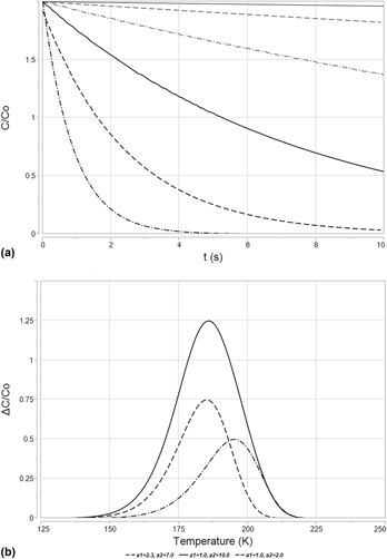
Carrier emission from a trap state is a thermally driven process. The emission rate changes with temperature and gives rise to a shift in ΔC/C O, as shown in Fig. 1(a). This leads to a peaked signal when ΔC/C O is plotted against temperature, T, as shown in Fig. 2(b). Variation in a 1 or a 2 settings will shift the peak position, as shown in Fig. 2(b). Shockley, Read, and Hall define the charge emission rate (e N) of a trap center in their treatment of nonradiative charge recombination in the presence of trap centers [Reference Shockley15]. This relationship is detailed in Eq. (2). The variable γT 2 represents the product of the density of states in the carrier band multiplied by the thermal velocity of the carrier under study [for holes in Si, γ = 1.02 × 10²² K−2/(cm2 s)]. The variable ΔE is the difference between the energy level of a trapped charge carrier and the energy level of a free charge carrier, either in the conduction band or into the valence band. The variable σ is the capture cross section of the trap and k is the Boltzmann’s constant,
 $${e_{\rm{N}}} = \sigma \gamma {T^2}{{\rm{e}}^{{{ - \Delta E} / {kT}}}}\quad .$$
(a) A set of simulated capacitance decay curves, plotted in terms of C/C O with respect to time after the beginning of the emission pulse, t. When sampling is performed at two separate times and the difference taken, the expression in Eq. (1) for ΔC/C O results. These particular capacitance decay curves were simulated using emission rates derived via Eq. (3), having a trap energy equal to E V + 0.3 eV (yielding a value of ΔE equal to 0.3 eV), σ = 1 × 10⁻¹⁵ cm2, and γ = 1.02 × 1022 cm−5/2. Though Eq. (1) assumes N T ≪ N A, N T is set equal to N A in this simulation to aid in plotting. For the sake of simplicity, this simulation is performed at a single value of t D, set equal to 1 × 10⁻⁴ s. Temperatures used to generate the various emission rates depicted in this figure ranged from 150 K to 200 K in steps of 10 K. (b) DLTS spectra plotted in terms of ΔC/C O with respect to temperature, T in Kelvins, from a trap simulated with the same physical characteristics as above, with t D = 1 × 10⁻⁴ s. The effect of emission rate variation with changing temperature is readily apparent. Variation in a 1 and a 2 gives rise to a shift in peak position with temperature and gives rise to variation in amplitude, as is shown in this figure.

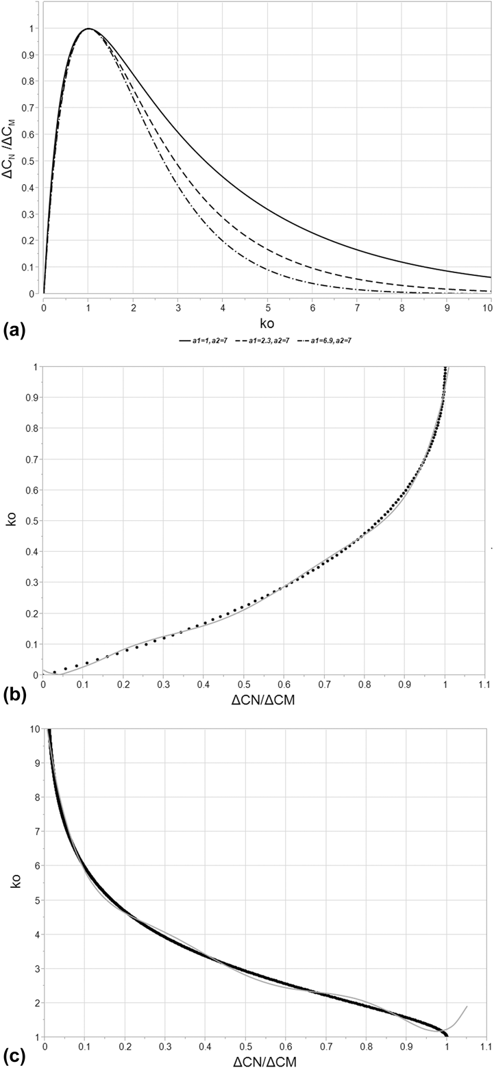
(a) A representative curve for k O versus ΔC N/ΔC M [Eq. (5)] for various a 1 and a 2 settings, both varying between 1 and 10. Of particular interest is the curve for a 1 = 2.3 and a 2 = 7.0, which correspond to the settings associated with the SULA DLTS system used for this study. Note that the function peaks at a value of 1 for both k O as well as ΔC N/ΔC M. This is the peak maximum, where e N is equal to e M. ΔC N decreases to either side of this peak maximum, driving toward zero. For k O < 1, this represents a value of e N < e M, corresponding to the “low temperature” side of the curve. For k O > 1, this represents a value of e N > e M, corresponding to the “high temperature” side of the curve. (b) The “low temperature” side of k O versus ΔC N/ΔC M [Eq. (5)] for a 1 = 2.3 and a 2 = 7.0, representing the settings associated with the SULA DLTS system used for this study. Also plotted in this figure is the polynomial fit to the relationship, explicitly recorded in Eq. (8) and Table I. R 2 = 0.997 for this fit. (c) The “high temperature” side of k O versus ΔC N/ΔC M [Eq. (5)] for a 1 = 2.3 and a 2 = 7.0, representing the settings associated with the SULA DLTS system used for this study. Also plotted in this figure is the polynomial fit to the relationship, explicitly recorded in Eq. (8) and Table I. R 2 = 0.997 for this fit.

A standard DLTS measurement makes use of multiple boxcar correlators, each set to a different t D, to measure the differential capacitance that results after the emission pulse begins. The changing t D defines a characteristic emission rate, e M, for the maximum of ΔC/C O, which can be derived by solving for the derivative of the DLTS signal with respect to emission rate and setting that derivative equal to zero. The result is the relationship detailed in Eq. (3) [Reference Lang1],
 $${e_{\rm{M}}} = {{\ln \left( {{{{a_2}} / {{a_1}}}} \right)} / {\left( {{t_{\rm{D}}}\left( {{a_2} - {a_1}} \right)} \right)}}\quad .$$
ΔE and σ for can be determined for trap emission observed via DLTS through an Arrhenius plotting method [Reference Lang1]. The temperature (T M) and emission rate (e M) at which ΔC/C O is maximized are compared against the t D settings associated with the measurement. By plotting the natural logarithm of  ${{{e_{\rm{M}}}} / {T_{\rm{M}}^2}}$, with respect to 1/kT M, an Arrhenius plot may be generated which yields a linear function. The slope of this function is equal to ΔE for the emission rate and the intercept with the vertical axis yields a value from which σ may be extracted.
Using an Arrhenius plot is an accurate means of deriving the characteristics of a deep level trap when no other DLTS signals are close enough to superimpose on the maximum of the peak. However, the method is very susceptible to distortion effects from superpositioning of peaks due to the assumption of a single-rate decay caused by only one deep level trap species. Arrhenius plots provide little means of avoiding this distortion effect because only the peak maximum is used to derive the necessary data for an Arrhenius plot. This was quickly recognized as a fundamental shortcoming of the standard DLTS technique. Alternatives to the Arrhenius plotting method do exist. Lang has proposed a means of measuring the activation energy of a trap from the full width at half maximum (FWHM) of a DLTS spectrum derived from DLTS measurements made with a lock-in amplifier [Reference Lang13]. A similar method for use with a boxcar correlator was developed by Goto et al. [Reference Goto, Adachi and Ikoma16]. Le Bloa et al. developed a means of measuring the emission rate independent of a temperature sweep using the Fourier transform [Reference Le Bloa, Quan and Guennouni17] and Peaker et al. performed a similar exercise using the Laplace transform [Reference Peaker, Markevich, Hawkins, Hamilton, Bonde Nielsen and Gościński18]. Other computational methods exist and are used frequently to de-convolve superimposed peaks generated by multiple DLTS transients, such as the method proposed by Hanine et al. [Reference Hanine and Masmoudi19].
In this paper, we introduce a new method to calculate ΔE and σ for electrically active deep level traps in a semiconductor by utilizing the capacitance transient data from a single correlator setting, t D. This is achieved by means of a function relating the relative displacement in temperature between the maximum of ΔC/C O and any point along the peak generated as part of the DLTS measurement. This function enables the accurate calculation ΔE, σ, and N T of an active deep level trap. Because of the way this function is derived, we believe that it is far less sensitive to distortion from emission signal superposition, potentially far more accurate than the Arrhenius plot in cases of such superposition, and easily integrated into existing computer programs used for DLTS signal analysis.
In this text, the peak shape normalized to the maximum (ΔC N/ΔC M) is utilized. In this term, ΔC M is equal to the differential capacitive DLTS signal at the peak maximum and ΔC N is the differential capacitive DLTS signal at an arbitrary point along the peak. The only variable contained within the emission rate for a given trap state (with a characteristic ΔE, σ, and γ) is the temperature at which the measurement is being made. Thus, a DLTS peak may be transformed from “temperature space” to “emission rate space” and back again at will and any point on a DLTS curve may be defined by an emission rate just as easily as it might be defined by temperature. To that end, the emission rate at any point along a DLTS peak arising from trap state emission, e N, is related to the emission rate at the point at which the maximum occurs, e M, by a function (k O) via Eq. (4),
 $${e_{\rm{N}}} = {k_{\rm{O}}}{e_{\rm{M}}}\quad .$$
In order to solve for k O, the equation for the curve shape of a DLTS peak must be transformed from “temperature space” to “emission rate space”. Recall that the expression for the DLTS peak as a function of the emission rate may be differentiated with respect to t D and set to zero to yield Eq. (3). Recall also that any emission rate along the curve may be related to the emission rate at the maximum through k O, per Eq. (4). By substituting Eqs. (3) and (4) into Eq. (1) and performing a little algebra to find for the ratio of ΔC N/ΔC M, an expression can be derived for ΔC N/ΔC M per Eq. (5). All of the variables in this equation are known excepting k O, which is obviously dependent upon the rate window as well as the point on the curve being sampled. It stands to reason, given this derivation for ΔC N/ΔC M, that k O that could be determined numerically for a given ΔC N/ΔC M,
 $$\eqalignb{{{\Delta {C_{\rm{N}}}} \over {\Delta {C_{\rm{M}}}}} = {{\left( {{{\left( {{{{a_2}} \over {{a_1}}}} \right)}^{ - {{{k_{\rm{O}}}{a_2}} \over {\left( {{a_2} - {a_1}} \right)}}}} - {{\left( {{{{a_2}} \over {{a_1}}}} \right)}^{ - {{{k_{\rm{O}}}{a_1}} \over {\left( {{a_2} - {a_1}} \right)}}}}} \right)} / }\cr{\left( {{{\left( {{{{a_2}} \over {{a_1}}}} \right)}^{ - {{{a_2}} \over {\left( {{a_2} - {a_1}} \right)}}}} - {{\left( {{{{a_2}} \over {{a_1}}}} \right)}^{ - {{{a_1}} \over {\left( {{a_2} - {a_1}} \right)}}}}} \right)}}\quad .$$
As shown in Fig. 2(a), the resulting function, described in Eq. (5), is peaked at the point where both ΔC N/ΔC M and k O are equal to one, this point being the maximum of the DLTS peak. The left hand side of the function corresponds to the low-temperature side of the DLTS peak, and it attenuates rapidly, reaching the point where both ΔC N/ΔC M and k O are equal to zero. Recall that k O is equal to e N/e M, which approaches zero as the temperature approaches 0 K. On the right hand side, the function attenuates slowly, only approaching a value of ΔC N/ΔC M equal to zero as k O approaches an infinite value, equivalent to an infinite temperature. As is readily observable, the left hand side of the function does not vary strongly with varying values of the machine constants a 1 and a 2. This is not the case on the right hand side of the equation. As the values of a 1 and a 2 separate, the magnitude of the function rises quickly.
Now that k O has been defined relative to ΔC N/ΔC M, the peak shape can be used to calculate ΔE and σ. Equation (6) results from the combination of Eqs. (2) and (4) along with some algebraic manipulation. For a single trap species, σ and γ are assumed to be constant and may be eliminated from the solution for ΔE. The form of this equation is critical as it demonstrates a means of measuring ΔE for a given DLTS peak that has no dependence on σ, assuming k O can be determined, which was shown previously in Eq. (4). By combining Eq. (6) with the expression for the emission rate at the peak maximum, e M [Eq. (2)], σ can also be derived per Eq. (7). This methodology is hereafter termed half width at variable intensity analysis, or HWVI, and it offers an attractive alternative to many other techniques used in DLTS when boxcar correlators are utilized. It can use data from anywhere along a given peak generated by DLTS (rather than only the maximum, as is the case in Arrhenius plotting), and it requires no iterative computation to determine the key physical characteristics of an observed trap,
 $$\Delta E = \ln \left( {{{{k_{\rm{O}}}T_{\rm{M}}^{\rm{2}}} \over {T_{\rm{N}}^{\rm{2}}}}} \right){\left( {{1 \over {k{T_{\rm{M}}}}} - {1 \over {k{T_{\rm{N}}}}}} \right)^{ - 1}}\quad ,$$
 $$\sigma = {{\ln \left( {{{{a_2}} / {{a_1}}}} \right)} / {\left( {{t_{\rm{D}}}\gamma T_{\rm{M}}^{\rm{2}}\left( {{a_2} - {a_1}} \right){{\rm{e}}^{{{ - \Delta E} / {k{T_{\rm{M}}}}}}}} \right)}}\quad .$$
As stated above, Eqs. (6) and (7) assume that σ is thermally independent. This is not always the case [Reference Zhao, Schlesinger and Milnes20, Reference Ozder, Atilgan and Katircioglu21]. Some capture cross sections have an exponential dependence on temperature or have their own characteristic activation energy. In the case of a thermally activated σ, its own component ΔE would have an additive distortion effect on Eq. (6), resulting in an observed energy gap between the trap energy and the conduction/valence band that is larger than physical reality. In practice, if the measured ΔE is dependent on ΔC N/ΔC M, or if there is a large variation in the calculated σ, it is possible that the root cause is a thermally dependent capture cross section. In cases where σ varies weakly with temperature, the impact on the calculation in Eqs. (6) and (7) can be assumed to be minimal. Large variation in σ invalidates the above equations.
The a 1 and a 2 values specified for the SULA DLTS system used during the experimental portion of this work are 2.3 and 7.0, respectively. By inputting these values into Eq. (5), k O can be estimated via a best-fit polynomial to the “low temperature” and “high temperature” sides of Eq. (5) per Eq. (8) and Table I,
 $${k_{\rm{O}}} = {N_0} + {N_1}{{\Delta {C_{\rm{N}}}} \over {\Delta {C_{\rm{M}}}}} + \sum\limits_{i = 2}^{i = 6} {{N_i}{{\left( {{{\Delta {C_{\rm{N}}}} \over {\Delta {C_{\rm{M}}}}} - C} \right)}^i}} \quad .$$
Constants associated with the polynomial fit for k O as a function of ΔC N/ΔC M, per Eq. (8) for T N < T M, shown in Fig. 2(b), and T N > T M in Fig. 2(c). N i values are expressed after the column expressing C, with N i values tabulated in descending order corresponding to their order along the top row.

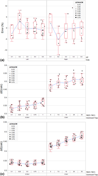
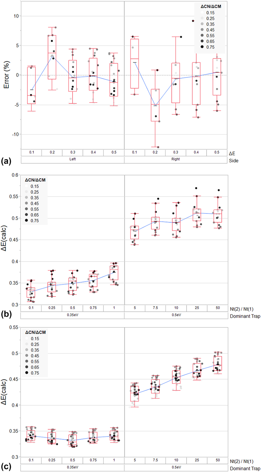
Figure 2(b) shows the polynomial fit for k O as a function of ΔC N/ΔC M compared to the “low temperature” side of Eq. (7), while Fig. 2(c) shows the polynomial fit for k O as a function of ΔC N/ΔC M compared to the “high temperature” side of Eq. (7). Both of these polynomial fits will clearly introduce some amount of error into the ΔE and σ measurements associated with this new technique. Figure 3(a) shows the “percent error” resulting from HWVI fitting of the “low-temperature” and “high temperature” curves of a simulated DLTS peak for a hole trap (with a constant t D and σ, and variable ΔE) over the undistorted region of the polynomial fit. Based on this exercise, fitting the “low temperature” side should result in a measurement with a standard deviation of 3.5% whereas fitting the “high temperature” side of a peak should result in a measurement with a standard deviation of 4.8%. The polynomial fit of the “low temperature” side of the peak is of a higher quality than the fit of the “high temperature” side of the peak. In cases where higher precision is required, a look-up table or some similar computational method could be implemented to effectively eliminate this error. As will be shown later, the residual error resulting even from the use of this admittedly crude polynomial fit is small relative to the error associated with the use of an Arrhenius plot.
(a) A plot of the calculated residual error resulting from the polynomial fit of k O to the “high temperature” and “low temperature” sides of Eq. (5), per Eq. (8) and Table I. The residual error is calculated by simulating a discrete hole trap (with t D = 1 × 10⁻⁴ s, σ = 1 × 10⁻¹⁵ cm2, and ΔE varying from 0.1 to 0.5 eV) and using a combination of Eqs. (5) and (6) to calculate ΔE over a range of ΔC N/ΔC M (0.2–0.8). The deviation between the calculated ΔE and nominal ΔE is normalized to the nominal ΔE to yield the residual error as a percentage of the nominal value. Mean values, inner quartile ranges, and six-sigma ranges are represented by the box plots. (b) Simulation of the superposition of a low-energy trap and a high-energy trap and the resulting distortion in HWVI calculated ΔE, arising from Eqs. (5), (6), and (8). (Trap 1 with ΔE = 0.35 eV, σ = 1 × 10⁻¹⁵ cm2, and N T = 1 × 1015 cm−3; Trap 2 with ΔE = 0.50 eV, σ = 1 × 10⁻¹² cm2, and N T ranging from 1 × 1015 cm−3 to 5 × 1017 cm−3). In this case, the calculation is made on the “low temperature” side of the peak. Mean values, inner quartile ranges, and six-sigma ranges are represented by the box plots. (c) Simulation of the superposition of a low-energy trap and a high-energy trap and the resulting distortion in HWVI calculated ΔE, arising from Eqs. (5), (6), and (8). (Trap 1 with ΔE = 0.35 eV, σ = 1 × 10⁻¹⁵ cm2, and N T = 1 × 1015 cm−3; Trap 2 with ΔE = 0.50 eV, σ = 1 × 10⁻¹² cm2, and N T ranging from 1 × 1015 cm−3 to 5 × 1017 cm−3). In this case, the calculation is made on the “high temperature” side of the peak. Mean values, inner quartile ranges, and six-sigma ranges are represented by the box plots.
As noted previously, when multiple trapping signatures are observed in tandem, superposition can interfere with proper trap identification. The effect of superposition is to generate a trap signal which must be considered as a single trap but which is, in actuality, the superposition of multiple traps. The result of this effect is that the derivation above, which assumes a single trap signal to calculate ΔE, may deviate from reality by a substantial margin.
Distortion via superposition is best avoided by adjusting the range of ΔC N/ΔC M over which ΔE is calculated as well as the “side” of the peak utilized for the calculation. This strategy can be used to effectively remove the distorted portions of the signal from the calculation. Wide windows are viable in spectra where trap signals are reasonably well-separated and even narrow windows can easily yield many individual calculations of ΔE and σ: a substantial improvement over conventional Arrhenius plot-based DLTS. Another possible solution to a superposition problem is to manually subtract a superimposed peak that has been successfully identified from the raw spectrum.
In situations where superposition does occur and cannot be avoided, distortion can definitely lead to misidentification. Figures 3(b) and 3(c) represent the simulation of an extreme case of superposition. For this simulation, two peaks are superimposed on one another with almost equal T M, but with a large difference in ΔE (0.35 eV for the low-energy trap and 0.50 eV for the high-energy trap). In Fig. 3(b), the “low temperature” side of the resulting superimposed peak is analyzed with HWVI as N T varies for the high-energy trap. In Fig. 3(c), the “high temperature” side of the resulting superimposed peak is analyzed with HWVI as N T varies on the high-energy trap.
In the case of analysis of the “low temperature” side of the resulting superimposed peak, the 0.35 eV trap is favored over the 0.50 eV trap, even when both traps possess equal N T. The presence of the 0.35 eV trap continues to influence the measurement of the 0.50 eV trap, even when N T of the 0.50 eV trap exceeds that of the 0.35 eV trap by 50×. The resulting standard deviation in measurement when N T for the 0.35 eV trap exceeds N T for the 0.50 eV trap is 5.6%, while the standard deviation in measurement when N T for the 0.50 eV trap exceeds N T for the 0.35 eV trap is 5.7%. In the case of the “high temperature” side of the resulting superimposed peak, analysis of the 0.50 eV trap results in an accurate measurement of ΔE, but only when N T for the 0.50 eV trap is more than 5× that of the 0.35 eV trap. When the 0.50 eV trap possesses a low N T, it still influences the measurement of the 0.35 eV trap, but not so much that the 0.35 eV trap would likely be misidentified. The resulting standard deviation in measurement when N T for the 0.35 eV trap exceeds N T for the 0.50 eV trap is 10.2%, while the standard deviation in measurement when N T for the 0.50 eV trap exceeds N T for the 0.35 eV trap is 5.5%. Based on these results, a few general observations can be made about how distortion influences HWVI analysis.
In a superposition situation, HWVI is more likely to detect the lower energy feature first, rather than the higher energy feature, regardless of the side measured. A large mismatch in concentration is required for an accurate measurement of ΔE for the higher energy feature. This means that low-energy features are easily identified by HWVI relative to obscuring high-energy features, which is somewhat advantageous in comparison to Arrhenius plots, where distortion from a broad, high-energy peak can easily skew a ΔE calculation. Unfortunately, this also means that low-energy features (such as interface states, for instance) can result in trap misidentification if a relatively high-energy peak does not have sufficient magnitude in the desired range of analysis.
Interestingly, analysis of the “high temperature” side of a peak favors accurate identification of high-energy traps relative to the “low temperature” side of a peak. Likewise, analysis of the “low temperature” side of a peak favors accurate identification of low-energy traps relative to the “high temperature” side of a peak. It seems that if analysis of the “low temperature” side of a peak results in a lower ΔE than the “high temperature” side of a peak, the “low temperature” ΔE measurement is more likely to be correct. Likewise, if analysis of the “high temperature” side of a peak results in a higher ΔE than the “low temperature” side of a peak, the “high temperature” measurement is more likely to be correct. In general, it also seems that HWVI tends to underestimate ΔE by a small margin if any superposition occurs.
In order to perform the HWVI fitting detailed in this work, each DLTS spectrum was smoothed using a linearly weighted running average function (termed ΔC avg/C O but hereafter treated as effectively equal to ΔC N/C O in all analysis). This reduced the noise in the ΔE and σ calculations by reducing error in determining the maximum of each peak, where the variation of ΔC/C O with respect to T approaches 0. The equation used to generate this linear weighting is as follows, per Eq. (9), where the “i” subscript denotes the current measurement,
 $${{\Delta {C_{{\rm{avg}}}}} \over {{C_{\rm{O}}}}} = {2 \over 5}\left( {{{\Delta {C_i}} \over {{C_{\rm{O}}}}} + {{3\Delta {C_{i - 1}}} \over {4{C_{\rm{O}}}}} + {{\Delta {C_{i - 2}}} \over {2{C_{\rm{O}}}}} + {{\Delta {C_{i - 3}}} \over {4{C_{\rm{O}}}}}} \right)\quad .$$
The following step-by-step procedure was used on all features in the resulting DLTS spectrum to extract all trap signals and to reconstruct the feature as a superposition of theoretical peaks derived from the HWVI analysis of this peak:
(i) The magnitude of the peak maximum and the temperature at which it occurs is identified.
(ii) ΔC N/ΔC M values of specific data points as well as the temperature at which these values occur are tabulated. The value of k O is computed from the polynomial fit to the function defining ΔC N/ΔC M in terms of k O, per Eqs. (5) and (8). ΔE and σ are computed from these values and from the temperatures at which they occur, using Eqs. (6) and (7), respectively.
(iii) The analyzed range of ΔC N/ΔC M is truncated to avoid distortion effects due to peak superposition or experimental noise. If needed, a theoretical DLTS peak generated from ΔE, σ, and a best-fit peak amplitude is subtracted from the observed signal in order to remove the superimposed contribution of the peak analyzed in Step 1 and Step 2.
(iv) Steps 1–3 are repeated until all large signals have been successfully characterized.
Results and discussion
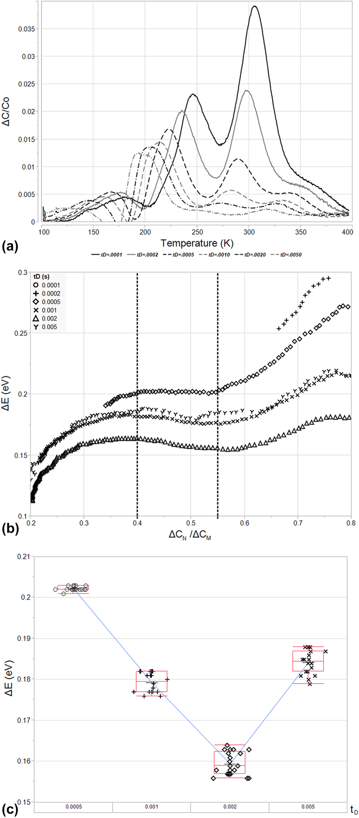
As shown in Fig. 4(a), analysis of the sample described in the Experimental section indicates the presence of three, separate, easily observed hole traps. Two of these occur at temperatures around 200 K, appearing as a single peak (Trap A) and a shoulder on the high temperature side (Trap B), while the third trap appears at a higher temperature of around 300 K (Trap C). It should be noted that the shouldered peak at approximately 200 K has been observed in the past during Ar+ ion implantation [Reference Mohapatra and Giri22]. The attenuation of DLTS signals at high delay times (which is a common issue for high-ΔE features) is particularly evident in this high temperature signal. The resultant attenuation reveals what appears to be a fourth trap level (Trap D) at temperatures ranging from 300 K to 350 K, depending upon t D.
(a) The DLTS spectra resulting from analysis of the B11 implanted structure described in section “Conclusions”. This structure was analyzed from t D settings ranging from 1 × 10⁻⁴ to 5 × 10⁻³ s and is plotted in terms of ΔC/C O versus T(K). Four peaks are evident: two (Trap A and Trap B, in order of lowest to highest temperature) situated between 150 and 250 K, and two peaks (Trap C and Trap D, in order of lowest to highest temperature) situated between 250 and 400 K. (b) Arrhenius plots resulting from analysis of peak temperature (1/kT M) versus peak emission rate in terms of peak temperature  $\left( {{{{e_{\rm{M}}}} / {T_{\rm{M}}^2}}} \right)$ for Trap A, Trap B, Trap C, and Trap D. The poor fitting of signals impacted by superposition (Trap B and Trap C especially) is evident.

Analysis of some of these traps, particularly Trap B and Trap D, is difficult due to the relative magnitude of these peaks and their proximity to Trap A and Trap C, respectively. Trap B’s and Trap D’s close neighbors obscure them at low values of t D, causing Trap D to appear only as a shoulder and completely engulfing Trap B up until a t D value of 1 × 10⁻⁴ s. Trap A and Trap C are also affected by their close proximity to Trap B and Trap D. The smaller traps possess a large enough amplitude to shift the maxima of Trap A and Trap C via superposition. The result is a distorted Arrhenius plot, demonstrated in Fig. 4(b). Trap A is ascribed to a deep level present at ΔE = 0.34 eV and σ = 2.77 × 10⁻¹⁶ cm2 via six datapoints, and the quality of this fit appears good, possessing R 2 = 0.999, but analysis with HWVI fitting will later show that this Arrhenius plot gives rise to an erroneous emission characteristic. Trap C fares little better and is ascribed to a deep level present at ΔE = 0.45 eV and σ = 3.45 × 10⁻¹⁷ cm2 via six datapoints, but the quality of the fit is obviously poor, possessing R 2 = 0.886. Trap B cannot truly be analyzed as the shoulder is obscured until the last t D setting, 1 × 10⁻⁴ s. Trap D is ascribed to a deep level present at ΔE = 1.01 eV and σ = 2.18 × 10⁻⁹ cm2 via only four datapoints due to its low amplitude compared to its neighbor, Trap C, but these values seem highly unrealistic. This would correspond to a macroscopic hole trap close to the Si conduction band.
Based on the analysis above, a DLTS operator would be forced to repeat the experiment performed at lower t D, if available, to attempt to remove the effects of superposition on Trap B and Trap D. The rate window being used is already quite short; however, an operator might find themselves forced to rely on other methods to attempt to tease out the behavior of these trap centers, such as altering the voltages used in the emission and filling pulses. In these cases, the region probed would shift as the quasistatic depletion regions generated by the emission pulse and filling pulse change. If N T varies with depth into the semiconductor for Trap A and Trap C, as might likely be the case for an implanted profile, this could cause attenuation and tease out the characteristics of Trap B and Trap D.
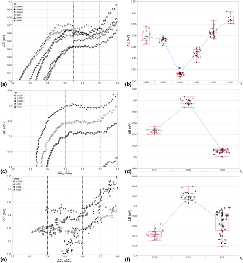
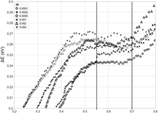
As shown in Figs. 5(a), 5(c), and 5(e), HWVI fitting can be used along the curve of each readily isolated DLTS peak to determine ΔE over a wide range of amplitudes. In Fig. 5(a), Trap A is analyzed over a window of 0.2 < ΔC N/ΔC M < 0.8 along its “low-temperature” side for all values of t D. This window captures a relatively stable section of the ΔE measurement, away from where Trap C distorts the measurement near the peak maximum, and away from the interface state background, where trap centers near the valence band dominate. The effect of the interface state background at low ΔC N/ΔC M is the same for Trap C, as shown in Fig. 5(c), where the trap is analyzed over the same window along its “low-temperature” side. Near the peak maximum, the polynomial fit begins to deviate from Eq. (5) and induces variation in the measured value of ΔE. The effect of interface states is much more pronounced during the analysis of the “high temperature” side of Trap D due to its reduced magnitude, resulting in severe distortion below ΔC N/ΔC M = 0.4. These results are omitted from the figure in order to focus on the variation in the undistorted regions of the peak. The influence of Trap C is also evident, causing distortion in the calculated ΔE at high ΔC N/ΔC M.
(a) The calculated values of ΔE for Trap A for 0.2 ΔC N/ΔC M < 0.8 and for all t D. From this plot, a stable reading for ΔE was verified for a range of 0.55 < ΔC N/ΔC M < 0.70. This range was used to calculate ΔE for all t D and is indicated by the dotted horizontal lines in the plot. (b) A variability plot of the resulting ΔE values used in calculation of the mean and t D-to-t D standard deviation for ΔE for Trap A. Mean values, inner-quartile ranges, and six-sigma ranges for each value of t D are represented by the box plots. (c) The calculated values of ΔE for Trap C for 0.2 ΔC N/ΔC M < 0.8 and for all t D. From this plot, a stable reading for ΔE was verified for a range of 0.50 < ΔC N/ΔC M < 0.70. This range was used to calculate ΔE for all t D < 1 × 10⁻³ s and is indicated by the dotted horizontal lines in the plot. (d) A variability plot of the resulting ΔE values used in calculation of the mean and t D-to-t D standard deviation for ΔE for Trap C in a range of t D < 1 × 10⁻³ s. Mean values, inner-quartile ranges, and six-sigma ranges for each value of t D are represented by the box plots. (e) The calculated values of ΔE for Trap D for 0.2 ΔC N/ΔC M < 0.8 and for t D > 2 × 10⁻⁴ s. From this plot, a stable reading for ΔE was verified for a range of 0.40 < ΔC N/ΔC M < 0.60. This range was used to calculate ΔE for 5 × 10⁻³ s > t D > 2 × 10⁻⁴ s and is indicated by the dotted horizontal lines in the plot. (f) A variability plot of the resulting ΔE values used in calculation of the mean and t D-to-t D standard deviation for ΔE for Trap D in a range of 5 × 10⁻³ s > t D > 2 × 10⁻⁴ s. Mean values, inner-quartile ranges, and six-sigma ranges for each value of t D are represented by the box plots.

For Trap A, all t D settings and a range of 0.55 < ΔC N/ΔC M < 0.70 are chosen to yield a calculation for ΔE via the “low-temperature” side of the peak. For Trap C, t D < 5 × 10⁻⁴ s is omitted due to interactions with Trap B (on the “low-temperature” side) and Trap D (on the “high temperature side”). A range of 0.50 < ΔC N/ΔC M < 0.70 is chosen to yield a calculation for ΔE via the “low-temperature” side of the peak. The “high temperature” side of Trap D is analyzed for 5 × 10⁻³ > t D > 2 × 10⁻⁴ s to avoid distortion by the interface state background (at t D > 5 × 10⁻³ s) and by Trap C (at t D < 2 × 10⁻⁴ s). A conservative range of 0.40 < ΔC N/ΔC M < 0.60 is chosen to further avoid distortion from interface states and neighboring traps. This corresponds to 107 measurements for Trap A, 81 measurements for Trap C, and 112 measurements for Trap D, a roughly 17× increase in measurement efficiency over the Arrhenius plotting method for six values of t D and three different trap centers.
The results of this analysis are shown in Fig. 5(b) for Trap A, Fig. 5(d) for Trap C, and Fig. 5(f) for Trap D, respectively. Trap A is found to possess a ΔE of 0.257 eV, with a standard deviation of 0.008 eV, and a resulting σ of 1.30 × 10⁻¹⁷ cm2, calculated from the log-averaged values of σ derived from ΔE per Eq. (6). The logarithmically weighted standard deviation in σ is equal to 0.51 orders of magnitude. The dopant-normalized trap concentration, N T/N A, is estimated to be equal to 5.34 × 10⁻², based on Eq. (1) for t D = 1 × 10⁻⁴ s, though it should be noted that this quantity decreases by 2× with decreasing t D. The trap center, itself, could be related to hydrogen interaction with vacancies in irradiated Czochralski silicon, though the DLTS spectra used in the cited work contained considerable superposition [Reference Felisova, Yarykin, Yakimov and Weber23]. Trap C is found to possess a ΔE of 0.551 eV, with a standard deviation of 0.043 eV, and a resulting σ of 5.49 × 10⁻¹⁵ cm2, with a logarithmically weighted standard deviation of 0.54 orders of magnitude. N T/N A is estimated to be equal to 5.04 × 10⁻² for t D = 5 × 10⁻⁴ s. The mean activation energy of this trap is within three standard deviations of the reported activation energy for a vacancy-hydrogen bond (VH3) [Reference Bruni, Bisero, Tonini, Ottaviani, Queirolo and Bottini24]. Trap D has a ΔE of 0.377 eV, with a standard deviation of 0.038 eV, and a resulting σ of 1.04 × 10⁻¹⁸ cm2, with a logarithmically weighted standard deviation of 0.52 orders of magnitude. Trap D appears at a higher temperature, relative to Trap C, due to its smaller capture cross section. N T/N A is estimated to be equal to 4.47 × 10⁻³ for t D = 5 × 10⁻⁴ s. This correlates well with previous reports of trap centers formed between the bonding of interstitial carbon and oxygen, though the Arrhenius plots associated with this attribution did not result in good linear fits in the literature [Reference Mooney, Cheng, Suli, Gerson and Corbett25].
It should be noted that the calculation for σ requires an accurate value of ΔE and is, therefore, not an independent measurement of the capture cross section and exponentially dependent upon noise in ΔE (resulting in the large standard deviations demonstrated above). For this reason, care must be taken in choosing the physical constants used in peak subtraction to expose Trap B for analysis. During subtraction, DLTS spectra can be simulated based on Eqs. (1) and (2) and these simulated spectra can then be subtracted from the raw spectra presented in Fig. 3(a). In this case, the signal for Trap A was simulated over all t D by setting ΔE = 0.267 eV (the mean ΔE for t D = 5 × 10⁻³ s), by setting σ = 6.58 × 10⁻¹⁸ cm2 (the logarithmic mean σ for t D = 1 × 10⁻⁴ s), and by varying N T/N A from 5.34 × 10⁻² to 2.18 × 10⁻² (matching calculated peak amplitudes for Trap A at each t D). The resulting simulated peaks were attenuated to a level of 75% of their calculated N T/N A concentrations for each given t D in order to avoid over-attenuating the raw signal. This subtraction yields Fig. 6(a). The maxima of Trap B are now apparent and can be used to analyze the trap using HWVI fitting. This is performed in the same fashion as above.
(a) The DLTS spectra resulting from the subtraction of a simulated Trap A DLTS spectrum from the raw DLTS spectra depicted in Fig. 3(a). The subtracted spectrum for Trap A is derived via Eqs. (1) and (3) for ΔE = 0.267 eV, σ = 6.58 × 10⁻¹⁸ cm2, and N T/N A varying from 5.34 × 10⁻² to 2.18 × 10⁻². (b) The calculated values of ΔE for Trap B for 0.2 ΔC N/ΔC M < 0.8 and for all t D. From this plot, a stable reading for ΔE was verified for a range of 0.40 < ΔC N/ΔC M < 0.55. This range was used to calculate ΔE for t D > 2 × 10⁻⁴ s and is indicated by the dotted horizontal lines in the plot. (c) A variability plot of the resulting ΔE values used in calculation of the mean and t D-to-t D standard deviation for ΔE for Trap D for t D > 2 × 10⁻⁴ s. Mean values, inner-quartile ranges, and six-sigma ranges for each value of t D are represented by the box plots.

In Fig. 6(b), Trap B is analyzed over a 0.2 < ΔC N/ΔC M < 0.8 along its “high temperature” side for all values of t D in order to avoid distortion from Trap A and from residual error in the polynomial fit to Eq. (5). A range of 0.40 < ΔC N/ΔC M < 0.55 is chosen to yield a calculation for ΔE via the “high temperature” side of the peak and signals with t D < 5 × 10⁻⁴ s are omitted due to interactions with Trap C. This corresponds to 87 measurements for Trap B, an impressive result given that Arrhenius plotting could only yield a single datum for analysis: not even enough to estimate ΔE or σ. The results of this analysis are shown in Fig. 6(c) for Trap B. The trap is found to possess a ΔE of 0.181 eV, with a standard deviation of 0.018 eV, and a resulting σ of 1.16 × 10⁻¹⁹ cm2, with logarithmically weighted standard deviation of 0.28 orders of magnitude. The dopant-normalized trap concentration, N T/N A, is estimated to be equal to 2.17 × 10⁻⁴ for t D = 5 × 10⁻⁴ s. Trap B appears at a higher temperature, relative to Trap A, due to its smaller capture cross section. Previous studies have suggested that the divacancy can form a trap center at E V + 0.17 eV [Reference Miller, Lang and Kimerling26, Reference Evwaraye and Sun27].
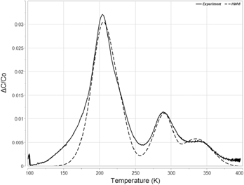
Figure 7 represents an effort to qualitatively represent the accuracy of the applied HWVI method in this particular experiment. A simulated spectrum based on the values of Traps A, B, C, and D is plotted against the experimental data for t D = 0.0005 s. The simulated data do not perfectly mimic the experimental data. Most notably, the experimental data are broader at the low and high temperature edges of both the Trap A/B feature and the Trap C/D feature. This suggests the presence of additional trap species at low concentrations, or perhaps distortion from an interface state background. Additionally, some fitting of the simulated data was required. The mean ΔE values for t D = 0.0005 s were used, rather than the calculated mean for all applicable t D. Additionally, for every trap species, σ was iterated within +/− one standard deviation of the mean value for t D = 0.0005 s, and N T/N A were allowed to vary freely until a best fit was found. Nevertheless, the data indicate that the HWVI methodology does produce results that appear reasonably accurate.
A comparison between experimental data collected at t D = 0.0005 s and a simulated spectrum derived from HWVI analysis of Trap A (ΔE = 0.24 eV, σ = 4 × 10⁻¹⁸ cm2, and N T/N A = 0.08), Trap B (ΔE = 0.20 eV, σ = 5 × 10⁻²⁰ cm2, and N T/N A = 0.10), Trap C (ΔE = 0.51 eV, σ = 2.3 × 10⁻¹⁵ cm2, and N T/N A = 0.05), and Trap D (ΔE = 0.34 eV, σ = 2.8 × 10⁻¹⁹ cm2, and N T/N A = 0.03).

Given the previous discussion regarding superposition, it bears noting that Trap A is taken from the “low temperature” side of the peak and has a higher ΔE than Trap B, which is taken from the “high temperature” side of the peak. Where this the only peak in the DLTS spectrum, a reversal of order of analysis might be warranted (i.e., analyzing the “high temperature” side of the peak for Trap A and then analyzing the “low temperature” side of the peak for Trap B). However, because peak subtraction of Trap A is required and because Trap B also interacts with Trap C, this reversal of order results in a much more distorted ΔE calculation than the initial methodology. Regardless, the difference in energy between Trap A and Trap B would imply only a few 0.01 eV of distortion of Trap A in the worst case, based on the simulations in Fig. 3.
It also bears noting that the trap species outlined above as possible sources for the observed traps in this study were first analyzed using DLTS and Arrhenius plots. This attribution engenders an admitted inconsistency. If trap superposition results in a condition where the Arrhenius plotting method breaks down, even when no obvious superposition is observed, then what historical data using Arrhenius plots can be trusted as accurate sources of energetic characteristics of trap species? We propose that any Arrhenius plot where scatter exists around a linear fit to the activation energy should be viewed with skepticism, though the experimental data above also demonstrate that an Arrhenius plot with a high R 2 cannot necessarily be trusted either. Any work where the Arrhenius plot is later verified using theoretical fitting of a simulated DLTS peak is likely accurate. The value of σ can also be a guide. A capture cross section can be said to describe a zone of interaction beyond which particles will not be affected by one another. If an atomistic defect is said to have a σ that is orders of magnitude larger than the area bounded by the proposed defect, the Arrhenius plot that led to this value of σ is likely inaccurate.
Conclusions
Analysis of the B11-implanted MOSCAP described above demonstrates the utility of HWVI fitting of DLTS spectra. Arrhenius plots suggested that Trap A, Trap C, and Trap D possessed energies of E V + 0.34 eV, E V + 0.45 eV, and E V + 1.01 eV, respectively. HWVI fitting demonstrated that ΔC/C O superposition due to interactions with both interface states as well as neighboring discrete energy states had resulted in distortion, causing the Arrhenius plots to inaccurately estimate the identified trap energies. HWVI was used to identify the true energies of Trap A (E V + 0.26 eV), Trap C (E V + 0.55 eV), and Trap D (E V + 0.38 eV). In addition, HWVI fitting and peak subtraction were used to identify the peak shoulder resulting from a fourth discrete energy level (Trap B = E V + 0.18 eV), where Arrhenius plots were unable to isolate from its neighboring energy levels. This successful reanalysis of the B11-implanted sample enabled the attribution of various trap species identified in the DLTS spectrum to a host of implant-related defects formed from vacancy interactions as well as interactions between carbon and oxygen present in Czochralski grown Si, though these attributions are admittedly questionable due to superposition and poor fitting in the literature.
It should be noted that, despite its flaws, boxcar correlation is still a widely adopted, if complementary, method for spectral collection in DLTS and is often utilized in the renewable energy sector [Reference Rosenberg, Legodi, Rakita, Cahen and Diale28, Reference Heo, Seo, Lee, Lee, Seol, Lee, Park, Kim, Yun, Kim, Shin, Ahn and Nazeeruddin29]. This is a testament to the ease of measurement and analysis provided by boxcar correlation and to the overall longevity and utility of DLTS as a means of characterizing novel semiconductor devices and materials. It seems that HWVI might further enhance the capabilities of boxcar correlation for DLTS analysis in a wide variety of cases where discrete energy levels are present in bulk semiconductor samples. While the above derivation is completed for a capacitive signal, its generality makes it useful in a variety of device structures, and for a variety of pulsing and sensing methods, whenever boxcar correlators are used for analysis. The fact that the analysis method utilizes a closed-form function greatly reduces reliance on computerized analysis or peak fitting, granting it a distinct advantage over many other modern DLTS analysis techniques and granting it backward compatibility with legacy DLTS instruments, which do not benefit from the relative advantages of techniques such as LDLTS. HWVI also presents a warning to researchers studying defects identified in past DLTS studies using boxcar correlators. Superposition of multiple defect states could render inaccurate many of the measurements made in these studies, even if spectra do not appear to suffer from the effects of superposition, as was the case in this work.
Experimental
The analysis, described in this work, was performed on a previously existing sample that had been analyzed using a traditional Arrhenius plotting approach. This sample was an MOS capacitor formed by dry oxidation at 900 °C for 40 min in a Bruce 7670 diffusion furnace with a mean oxide thickness of 19.7 nm on a P-Type Si substrate with a (100) orientation and a resistivity in the range of 8–15 Ω-cm. This thin oxide was chosen as an alternative contacting scheme to a Schottky diode because of its exceptionally low leakage current and because the thin nature of this oxide reduces the capacitive signal from interface states to a magnitude that is much less than the capacitive signal from bulk traps [Reference Whiting30].
After oxide growth, ion implantation was performed using the B11 isotope extracted from BF3. This ion implantation was performed in a Varian 350D Ion Implanter with a tilt of 7° and a rotation of 45°. The energy used for the ion implantation step was equal to 45 keV, resulting in a projected range of 142 nm and a straggle of 45 nm, as calculated by SRIM 2008™. The fluence associated with the implant was 2 × 10¹¹ ions/cm2. This low dose was used for two reasons. First, it minimized the damage to the oxide capping layer, ensuring that it would remain an effective insulator. Second, this low dose ensured that the number of injected defects would remain several orders of magnitude lower than the background doping of the silicon substrate, ensuring that large numbers of ionized defects would not distort the resultant spectrum and that the above derivation would remain valid.
Following ion implantation, the sample was coated with FujiFilm HPR504 photoresist and immersed in a buffered oxide etch (BOE) with a 6:1 stoichiometric ratio of HF to ammonium fluoride (NH4F). BOE etching occurred for a total of 20 min. During this time, the rear side of the sample was etched to denude the surface of any oxide formed during thermal growth. The photoresist was removed after this step using a Branson Model 3200 Asher and aluminum electrodes were thermally evaporated in a CV-18 evaporator. 200 nm of aluminum was deposited onto the front and back portions of the wafer in order to form “gate” and “ground” contacts. A shadow mask was utilized to maintain a uniform gate electrode diameter of approximately 1 mm.
Analysis of the sample was performed with a SULA Technologies Deep Level Transient Spectrometer with six independent boxcar correlators that were manually set to t D values varying from 1 × 10⁻⁴ to 5 × 10⁻³ s. The temperature range of the scan was set from 100 to 400 K. The voltage applied to the gate contact of the device was set to −1.1 V for the filling pulse (putting the device in a flat-band condition) and −0.7 V for the emission pulse (placing the device just barely at the threshold of inversion). This generated a depletion region of approximately 690 nm in the device at room temperature, leading to an equilibrium capacitance of 108 pF. The leakage current within the device remained small after implant, even at room temperature, equaling approximately 37 nA at 5 V. Prior to the DLTS measurement, the voltage conditions listed above were briefly inspected at 100 K in order to verify that the device was not biased into accumulation due to shifts in the flatband voltage induced by interface state freeze-out. However, it is very likely that the flatband voltage did shift during the temperature sweep so that the depletion width probed varied somewhat during the DLTS measurement. This may have resulted in some temperature-based variation in C N/C O. Depletion width variation with temperature would impact C O as well as the average value of N T. We assume that this distortion was small, however, because our temperature sweep was not low enough to induce freeze-out of shallow donors or acceptors, which tend to comprise the bulk of most interface state energy distributions.
Acknowledgments
The authors acknowledge Corning, Inc., for funding this research and for the use of their DLTS system. The Semiconductor and Microsystem Fabrication Laboratory at Rochester Institute of Technology is acknowledged for use of their facilities in generating the sample used for analysis in this study.