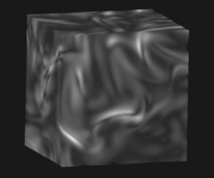

1. Introduction
At macroscopic scales, fluid dynamics is governed by partial differential equations that characterize the behaviour of a fluid in terms of fields that represent density, momentum and other locally conserved quantities. The evolution of these fields is given by fluxes that are modelled at the macro scale as smooth continuous functions of space and time. However, at atomic scales, fluids are discrete systems composed of individual molecules with complex interactions resulting in stochastic dynamics (e.g. Brownian motion). These two descriptions overlap at the meso scale. While it is possible to describe a fluid using macroscopic field variables at the meso scale, the fluxes are no longer smooth; instead, they include spontaneous thermal fluctuations even for systems that are at thermodynamic equilibrium.
Turbulent fluctuations are of a completely different origin. They are produced from the nonlinear cascade of energy due to external forcing at large length scales down to the scale of viscous dissipation. Below the length scale of the external forcing, the energy spectrum of turbulent fluctuations has two regimes, inertial and dissipative. The demarcation between them is determined by the Kolmogorov length scale  $\eta \equiv (\nu ^3/\langle \epsilon \rangle )^{1/4}$, where
 $\nu$ is the kinematic viscosity, and
 $\langle \epsilon \rangle$ is the mean energy dissipation rate. In the inertial range (wavenumber
 $k \ll k_{\eta } \equiv 2{\rm \pi} /\eta$) the energy spectrum has the form (Kolmogorov Reference Kolmogorov1941; Batchelor Reference Batchelor1953)
 $E(k) \propto k^{-5/3}$, while in the dissipative range it is often modelled as
 $E(k) \propto k^\alpha \exp ( - \beta k )$ (Frisch & Kolmogorov Reference Frisch and Kolmogorov1995; Pope Reference Pope2001; Buaria & Sreenivasan Reference Buaria and Sreenivasan2020). Since
 $E(k)$ decreases exponentially in the dissipative range, it is natural to ask: at what wavenumber do mesoscopic thermal fluctuations have a significant effect on this spectrum? This question dates back to the pioneering work of Betchov (Reference Betchov1957; Reference Betchov1961) and has received renewed attention in recent theoretical studies (Bandak et al. Reference Bandak, Eyink, Mailybaev and Goldenfeld2021; Eyink et al. Reference Eyink, Bandak, Goldenfeld and Mailybaev2021) and molecular simulation work (Gallis et al. Reference Gallis, Torczynski, Krygier, Bitter and Plimpton2021).
To investigate the influence of thermal fluctuations on turbulence, we turn to the theory of fluctuating hydrodynamics (FHD), originally proposed by Landau & Lifshitz (Reference Landau and Lifshitz1959). This theory extends conventional hydrodynamics by augmenting each dissipative flux with a random field. Over the past decade, our group and others have extended FHD, combining the derivation of models for complex fluids at the meso scale with the development of numerical algorithms for solving the resulting systems on high-performance computers. For example, we developed low-Mach-number stochastic FHD models for isothermal non-ideal liquid mixtures that exploit the separation of scales between fluid motion and acoustic wave propagation (Nonaka et al. Reference Nonaka, Sun, Bell and Donev2015). It has been demonstrated that this methodology can model accurately a wide range of phenomena both near and far from equilibrium (e.g. the experimentally observed ‘giant fluctuations’ effect in fluid mixing (Donev et al. Reference Donev, Bell, de La Fuente and Garcia2011)).
In this paper, we use fluctuating hydrodynamics to investigate the effect of thermal fluctuations in the dissipation range for homogeneous isotropic turbulence. Section 2 summarizes the formulation of incompressible FHD and estimates the wavenumber at which thermal fluctuations dominate turbulent fluctuations in the energy spectrum. Section 3 outlines the numerical algorithm of the simulations, and § 4 presents their results. In brief, the simulations confirm that thermal fluctuations dominate the energy spectrum at length scales comparable to the Kolmogorov length and produce nearly Gaussian velocity statistics at somewhat smaller scales.
2. Fluctuating hydrodynamics with forcing
In fluctuating hydrodynamics, we write the incompressible isothermal stochastic Navier–Stokes equations as
 \begin{equation} \left. \begin{gathered} \partial_t (\rho \boldsymbol{u} ) ={-}\boldsymbol{\nabla}\boldsymbol{\cdot}(\rho\boldsymbol{u}\boldsymbol{u}^{{\rm T}}) - \boldsymbol{\nabla} {\rm \pi}-\boldsymbol{\nabla}\boldsymbol{\cdot}(\bar{\boldsymbol{\tau}}+\tilde{\boldsymbol{\tau}}) + \rho\, \boldsymbol{a}^F(\boldsymbol{r},t),\\ \boldsymbol{\nabla} \boldsymbol{\cdot} \boldsymbol{u} = 0, \end{gathered} \right\} \end{equation}
where  $\boldsymbol {u}$ is the velocity,
 $\rho$ is the density,
 ${\rm \pi}$ is a perturbational pressure that enforces the divergence constraint, and
 $\boldsymbol {a}^F$ is a long-wavelength acceleration. Here, the deterministic stress tensor is
 $\bar {\boldsymbol {\tau }} = -\mu [\boldsymbol {\nabla } \boldsymbol {u} + (\boldsymbol {\nabla } \boldsymbol {u})^{\textrm {T}}]$ with dynamic viscosity
 $\mu$. The stochastic stress tensor chosen according to the fluctuation–dissipation relation (Landau & Lifshitz Reference Landau and Lifshitz1959; De Zarate & Sengers Reference De Zarate and Sengers2006) is
 \begin{equation} \tilde{\boldsymbol{\tau}} = \sqrt{\mu k_B T}\ (\boldsymbol{\mathcal{W}} + \boldsymbol{\mathcal{W}}^{{\rm T}} ), \end{equation}
where  $\boldsymbol {\mathcal {W}}$ is a standard white noise Gaussian tensor with uncorrelated components and
 $k_B$ is the Boltzmann constant. It is important to note that the stochastic stress tensor is only ‘quasi-white’ in space–time (Eyink et al. Reference Eyink, Bandak, Goldenfeld and Mailybaev2021). In particular, the fluctuating Landau–Lifschitz equations are not continuum stochastic PDEs but instead are a mesoscopic description, as made clear by derivations from microscopic descriptions based on Zwanzig–Mori projection-operator techniques (Zubarev & Morozov Reference Zubarev and Morozov1983; Español, Anero & Zúñiga Reference Español, Anero and Zúñiga2009).
The long-wavelength acceleration,  $\boldsymbol {a}^F$, due to an external force added to drive turbulence, is modelled here using the formulation of Eswaran & Pope (Reference Eswaran and Pope1988). Define an Ornstein–Uhlenbeck (OU) process for the complex vector
 $\boldsymbol {b}({\boldsymbol {n}} , t)$ as
 \begin{equation} {\rm d}\boldsymbol{b}({\boldsymbol{n}}) = \boldsymbol{A}\,\boldsymbol{b}({\boldsymbol{n}})\,{\rm d}t + \boldsymbol{B} \,{\rm d}\boldsymbol{{W}}, \end{equation}
where  ${\boldsymbol {n}} = (n_x, n_y, n_z)$ are integer indexes such that
 $1 \leq | {\boldsymbol {n}} | \leq n_{max}$ and
 $\boldsymbol {{W}}$ is a vector of complex Wiener processes. The external forcing is limited to long wavelengths by taking
 $n_{max} = 2\sqrt {2}$. The matrices in the OU process are taken to be
 \begin{equation} \boldsymbol{A} = \frac{1}{T_L}\,\boldsymbol{I}, \quad \boldsymbol{B} = \sigma \sqrt{\frac{1}{T_L}}\,\boldsymbol{I}, \end{equation}
where  $\boldsymbol {I}$ is the identity matrix. In this case, we have (Gardiner Reference Gardiner1985)
 \begin{equation} \langle \boldsymbol{b}({\boldsymbol{n}},t) \boldsymbol{\cdot} \boldsymbol{b}^*({{\boldsymbol{n}}'},t + s) \rangle = \frac{\sigma^2}{2}\,{\rm e}^{- s/T_L}\,\delta_{{\boldsymbol{n}},{\boldsymbol{n}}'}, \end{equation}
so the parameters  $T_L$ and
 $\sigma$ are the characteristic time scale and amplitude of the acceleration due to the external forcing. We then define the forcing in real space as
 \begin{equation} \boldsymbol{a}^F (\boldsymbol{r},t) = \mathrm{Re} \left[ \sum_{|{\boldsymbol{n}}| \leq n_{max}} (\boldsymbol{b}({\boldsymbol{n}}) + \boldsymbol{b}^*({-{\boldsymbol{n}}}) ) \exp({\mathrm{i} \, \boldsymbol{k} \boldsymbol{\cdot} \boldsymbol{r}}) \right ], \end{equation}
where  $\boldsymbol {k} = 2{\rm \pi} {\boldsymbol {n}}/L$,
 $L$ is the domain length, and
 $\mathrm {Re}$ denotes the real part of a complex number. Note that the enforcement of the divergence-free constraint on
 $\boldsymbol {a}^F$ is handled automatically by the solution algorithm.
On a periodic cubic domain  $[0,L]^3$, the velocity field,
 $\boldsymbol {u}(\boldsymbol {r})$, can be represented as a Fourier series
 \begin{equation} {\boldsymbol{u}}( \boldsymbol{r} ) = \sum_{\boldsymbol{k}} \hat{\boldsymbol{u}}_{\boldsymbol{k}} \exp({\mathrm{i} \boldsymbol{k} \boldsymbol{\cdot} \boldsymbol{r}}), \end{equation}
where  $\boldsymbol {k}\in (2{\rm \pi} /L)\, \mathbb {Z}^3$. The specific energy density in mode
 $\boldsymbol {k}$ is
 $E(\boldsymbol {k}) = \frac {1}{2}L^3\langle \hat {\boldsymbol {u}} _{\boldsymbol {k}}\boldsymbol {\cdot }\hat {\boldsymbol {u}}^*_{\boldsymbol {k}}\rangle$. The turbulent kinetic energy is then
 $\mathcal {E} = ({1}/{(2{\rm \pi} )^3})\sum _{\boldsymbol {k}} (\Delta k)^3 E(\boldsymbol {k}),$ with
 $\Delta k=2{\rm \pi} /L$. The specific dissipation rate is
 \begin{equation} \langle\epsilon\rangle = \nu \left\langle \frac{\partial u_i}{\partial x_j}\,\frac{\partial u_i}{\partial x_j} \right\rangle ={-} \nu \langle u_j \nabla^2 u_j \rangle = \nu \sum_{\boldsymbol{k}}| \boldsymbol{k} |^2 \left\langle\hat{\boldsymbol{u}}_{\boldsymbol{k}} \boldsymbol{\cdot} \hat{\boldsymbol{u}}^*_{\boldsymbol{k}}\right\rangle , \end{equation}
where  $\nu = \mu /\rho$ is the kinematic viscosity.
In the absence of forcing, the deterministic Navier–Stokes equations can be characterized in terms of a single parameter, namely, the Reynolds number  ${Re} = {U L}/{\nu }$, where
 $U$ and
 $L$ are characteristic velocities and length scales, respectively. (In the present setting, we can consider the forcing to simply be an, albeit indirect, approach to setting the velocity scale.) It is also useful to define the turbulence Reynolds number
 ${Re}_{T} = \mathcal {E}^2/(\langle \epsilon \rangle \nu )$ and the Taylor-scale Reynolds number
 ${Re}_{\lambda } = (\frac {20}{3} {Re}_{T})^{1/2}$.
Without forcing, the energy spectrum at long times for (2.1) is dominated by the effect of thermal fluctuations. These fluctuations can be characterized by the covariance of the velocity field at equilibrium, which is typically referred to as the velocity structure factor. Assuming that equilibrium mean flow is zero ( $\langle \boldsymbol {u} \rangle = 0$), the fluctuation–dissipation relation for the stochastic dynamics (2.1) implies, in agreement with Einstein–Boltzmann theory, that
 \begin{equation} L^3 \left\langle \hat{ \boldsymbol{u}}_{\boldsymbol{k}} \otimes \hat{\boldsymbol{u}}_{\boldsymbol{k}}^*\right\rangle = S_{\boldsymbol{u},\boldsymbol{u}} (\boldsymbol{k} ) = \frac{k_B T}{ \rho} \left ( \boldsymbol{I} - \frac{\boldsymbol{k} \boldsymbol{k}^{{\rm T}}}{|k|^2} \right ). \end{equation}
The contribution of fluctuations to the energy spectrum is then given by
 \begin{equation} {E^{{fluc}}(\boldsymbol{k}) = \frac{1}{2}L^3 \left\langle \hat{ \boldsymbol{u}}_{\boldsymbol{k}} \boldsymbol{\cdot} \hat{ \boldsymbol{u}}^*_{\boldsymbol{k}}\right\rangle = \frac{1}{2}\,\mathrm{Tr}( S_{\boldsymbol{u},\boldsymbol{u}} )= \frac{k_B T}{ \rho} .} \end{equation}
We note that this contribution is independent of  $\boldsymbol {k}$. Consequently, in the energy spectrum, fluctuations scale like
 $E(k) \propto k^2$, reflecting the scaling of surface area with radius. We note that the spatial discretization employed in this work is constructed so that this result remains exactly true in continuous time (Delong et al. (Reference Delong, Griffith, Vanden-Eijnden and Donev2013) and supplementary material available at https://doi.org/10.1017/jfm.2022.188) and with any discrete time step
 $\Delta t$ for the linearized dynamics (Usabiaga et al. Reference Usabiaga, Bell, Delgado-Buscalioni, Donev, Fai, Griffith and Peskin2012).
We note that the thermal energy spectrum,  $E^{fluc}(\boldsymbol {k}),$ does not have an ‘ultaviolet catastrophe’ (does not diverge when integrated over all
 $\boldsymbol {k}$) because there is an upper limit to the wavenumber given by the molecular scale. This upper bound for
 $k$ is related directly to the breakdown of the continuum description described in the last paragraph of this section.
The presence of thermal fluctuations introduces another scale into the problem. This additional dependence can be characterized in terms of a dimensionless temperature
 \begin{equation} \theta_\eta = \frac{k_B T}{\rho u_{\eta}^2 \eta^3} = \frac{k_B T \langle\epsilon\rangle^{{1}/{4}}}{ \rho \nu^{{11}/{4}}}, \end{equation}
where  $u_{\eta } = (\langle \epsilon \rangle \nu )^{1/4}$ is the Kolmogorov velocity. An order of magnitude estimate for the crossover wavenumber,
 $k_{\theta }$, between the turbulence spectrum and the thermal fluctuation spectrum is given by (Bandak et al. Reference Bandak, Eyink, Mailybaev and Goldenfeld2021; Eyink et al. Reference Eyink, Bandak, Goldenfeld and Mailybaev2021)
 \begin{equation} u_{\eta}^2 \eta \exp( - \beta k_{\theta} \eta ) \approx \frac{k_B T}{\rho}\,k_{\theta}^2, \end{equation}
where  $\beta$ is typically in the range 3–7 in the far-dissipation range (Khurshid, Donzis & Sreenivasan Reference Khurshid, Donzis and Sreenivasan2018). In terms of the Lambert
 $W$-function (Corless et al. Reference Corless, Gonnet, Hare, Jeffrey and Knuth1996),
 \begin{equation} k_{\theta} = \frac{2}{\beta \eta}\,W\left({\textstyle \frac12} \beta/\sqrt{\theta_\eta}\right) \approx \frac{2}{\beta \eta} \ln\left({\textstyle \frac12} \beta/\sqrt{\theta_\eta}\right) \end{equation}
for large arguments of  $W(x)$. For
 $\beta = 5$, the estimated crossover wavenumber for
 $\theta _\eta = 10^{-9}$ is
 $k_{\theta } = 3.6 / \eta = 0.58 k_{\eta }$, and for
 $\theta _\eta = 10^{-6}$ it is
 $k_{\theta } = 2.4 / \eta = 0.38 k_{\eta }$. Given that
 $\theta _\eta \approx 10^{-7}\text{--}10^{-8}$ in the atmospheric boundary layer and in laboratory experiments (Debue et al. Reference Debue, Kuzzay, Saw, Daviaud, Dubrulle, Canet, Rossetto and Wschebor2018), this result predicts that thermal fluctuations are significant at scales comparable to the Kolmogorov length scale. In cryogenic studies of turbulence, the dimensionless temperature is actually higher; for example,
 $\theta _\eta \approx 5.5\times 10^{-5}$ in the SHREK experiment (Kharche et al. Reference Kharche, Bon-Mardion, Moro, Peinke, Rousset and Girard2018).
The continuum description of fluid transport, either macroscopic or mesoscopic, is not accurate at molecular scales (Corrsin Reference Corrsin1959; Moser Reference Moser2006). This breakdown occurs below the microscopic transport length scale,  $\lambda _{mic}$; its ratio to the Kolmogorov length scale is
 \begin{equation} \frac{\lambda_{mic}}{\eta} = C\,\frac{{Ma}}{{Re}_{T}^{1/4}}, \end{equation}
where  ${Ma}$ is the Mach number, and
 $C$ is a constant of order 1. In dilute gases
 $\lambda _{mic}$ is the mean free path between collisions, and in liquids it is the intermolecular spacing. This result shows that
 $\eta \gg \lambda _{mic}$ for subsonic, high-Reynolds-number turbulence. Since laboratory experiments and molecular simulations have shown that (2.1) are accurate down to scales comparable to
 $\lambda _{mic}$ (Boon & Yip Reference Boon and Yip1991; De Zarate & Sengers Reference De Zarate and Sengers2006; Donev et al. Reference Donev, Vanden-Eijnden, Garcia and Bell2010, Reference Donev, Bell, de La Fuente and Garcia2011), we use them in our numerical simulations to validate the crossover wavenumber predicted by (2.13).
3. Simulation method
The fluctuating hydrodynamic simulations in this paper use the numerical method described in Nonaka et al. (Reference Nonaka, Sun, Bell and Donev2015). We use a staggered-grid formulation where normal velocities are stored on the normal faces of grid cells. We begin the time step with  $\boldsymbol {u}^n$. We evaluate a Stokes predictor to solve for a preliminary time-advanced velocity,
 $\boldsymbol {u}^{\star,n+1}$:
 \begin{align} \rho\,\frac{\boldsymbol{u}^{{\star},n+1}-\boldsymbol{u}^n}{\Delta t} + \boldsymbol{\nabla}{\rm \pi}^{{\star},n+1} &={-}\boldsymbol{\nabla}\boldsymbol{\cdot}(\rho\boldsymbol{u}\boldsymbol{u})^n - \frac{1}{2}\boldsymbol{\nabla}\boldsymbol{\cdot}\bar{\boldsymbol{\tau}}^n - \frac{1}{2}\boldsymbol{\nabla}\boldsymbol{\cdot}\bar{\boldsymbol{\tau}}^{{\star},n+1}\nonumber\\ &\quad + \boldsymbol{\nabla}\boldsymbol{\cdot}\left(\sqrt{\frac{\mu k_B T}{\Delta t\,\Delta V}}\,\bar{\boldsymbol{\mathcal{Z}}}^n\right) + \boldsymbol{a}^{F,n}, \end{align}
 \begin{align} \boldsymbol{\nabla}\boldsymbol{\cdot}\boldsymbol{u}^{*,n+1} &= 0, \end{align}
where  $\Delta V$ is the cell volume, and
 $\bar {\boldsymbol {\mathcal {Z}}} = \boldsymbol {\mathcal {Z}}+\boldsymbol {\mathcal {Z}}^{\textrm {T}}$, where
 $\boldsymbol {\mathcal {Z}}$ is a tensor containing unit-variance mean-zero independent Gaussian random variables.
We then evaluate a Stokes corrector to solve for the time-advanced velocity,  $\boldsymbol {u}^{n+1}$:
 \begin{align} \rho\,\frac{\boldsymbol{u}^{n+1}-\boldsymbol{u}^n}{\Delta t} + \boldsymbol{\nabla}{\rm \pi}^{n+1} &={-}\frac{1}{2}\boldsymbol{\nabla}\boldsymbol{\cdot}(\rho\boldsymbol{u}\boldsymbol{u})^n - \frac{1}{2}\boldsymbol{\nabla}\boldsymbol{\cdot}(\rho\boldsymbol{u}\boldsymbol{u})^{{\star},n+1} - \frac{1}{2}\boldsymbol{\nabla}\boldsymbol{\cdot}\bar{\boldsymbol{\tau}}^n - \frac{1}{2}\boldsymbol{\nabla}\boldsymbol{\cdot}\bar{\boldsymbol{\tau}}^{n+1}\nonumber\\ &\quad + \boldsymbol{\nabla}\boldsymbol{\cdot}\left(\sqrt{\frac{\mu k_B T}{\Delta t\Delta V}}\,\bar{\boldsymbol{\mathcal{Z}}}^n\right)+ \boldsymbol{a}^{F,n}, \end{align}
 \begin{align} \boldsymbol{\nabla}\boldsymbol{\cdot}\boldsymbol{u}^{n+1} &= 0. \end{align}
The only significant difference from this earlier work (Nonaka et al. Reference Nonaka, Sun, Bell and Donev2015) is the addition of the external forcing described in the previous section. For this external forcing calculation, (2.3), we use a simple Euler–Maruyama method; a higher accuracy integrator is not needed in this context since we are generating a random forcing. Starting with the initial condition  $\boldsymbol {b}^0 = (0, 0, 0)^{\textrm {T}}$, we advance (2.3) using
 \begin{equation} \boldsymbol{b}^{n+1} = \boldsymbol{b}^n + \boldsymbol{A} \boldsymbol{b}^n\,\Delta t + \boldsymbol{B} \sqrt{\Delta t}\,\boldsymbol{{Z}}^n\boldsymbol{I}, \end{equation}
where we advance  $\boldsymbol {b}({\boldsymbol {n}})$ only for values of
 ${\boldsymbol {n}}$ needed to compute
 $\boldsymbol {a}^F$. Here,
 $\boldsymbol {{Z}}$ is a complex Gaussian (normal) distributed random number. We can then evaluate
 $\boldsymbol {a}^{F,n}$ directly from
 $\boldsymbol {b}^n$ using (2.6).
4. Simulation results
We ran simulations with  $\rho = 1.0\,\mathrm {g}\,\mathrm {cm}^{-3}$,
 $T = 300$ K,
 $\mu =0.02$ poise, which corresponds to a water–glycerol mixture (Segur & Oberstar Reference Segur and Oberstar1951), in a (5.12 cm)
 $^3$ periodic domain with a
 $1024^3$ grid using a time step
 $\Delta t = 5 \times 10^{-5}$ s. Simulations using a
 $512^3$ grid (not shown) gave essentially the same results, which indicates that the simulations presented here are well resolved.
We considered two cases. In each case, we ran the simulation until it became statistically stationary ( ${\approx }30\,000$ steps). We then restarted the simulations with and without thermal fluctuations and ran for several thousand time steps. For these simulations, we compute the energy dissipation rate using the discrete Laplacian used in the numerical algorithm. Thus we capture the actual discrete energy dissipation to machine precision.
Case 1 has strong forcing ( $\sigma = \sqrt {10}\,\mathrm {cm}\,\mathrm {s}^{-2}$), and Case 2 has weak forcing (
 $\sigma = \sqrt {0.1}\,\mathrm {cm}\,\mathrm {s}^{-2}$); in both cases, the forcing time scale is
 $T_L = 0.1$ s. In Case 1, the mean energy dissipation rate is
 $\langle \epsilon \rangle \approx {17.7}\,\mathrm {cm}^2\,\mathrm {s}^{-3}$, resulting in Kolmogorov length and time scales
 $\eta = {0.025}$ cm and
 $\tau _{\eta } = (\nu /\langle \epsilon \rangle )^{1/2} = {0.033}$ s, respectively. The turbulent kinetic energy is
 $\mathcal {E} = 14\,\mathrm {cm}^2\,\mathrm {s}^{-2}$, which corresponds to
 ${Re}_{T} \approx {554}$ and
 ${Re}_{\lambda } \approx {61}$. For the Case 2 simulations (weak forcing), the mean energy dissipation
 $\langle \epsilon \rangle \approx {1.0}\,\mathrm {cm}^2\,\mathrm {s}^{-3}$ resulting in Kolmogorov length and time scales of
 $\eta = {0.053}$ cm and
 $\tau _{\eta } = {0.14}$ s, respectively. The turbulent kinetic energy is
 $\mathcal {E} = 1.9 \,\mathrm {cm}^2\,\mathrm {s}^{-2}$, corresponding to
 ${Re}_{T} \approx {180}$ and
 ${Re}_{\lambda } \approx {35}$. By comparison,
 $\langle \epsilon \rangle$ ranges from 400 to 156 000
 $\,\mathrm {cm}^2\,\mathrm {s}^{-3}$ in the water–glycerol experiments of Debue et al. (Reference Debue, Kuzzay, Saw, Daviaud, Dubrulle, Canet, Rossetto and Wschebor2018), while in geophysical flows,
 $\langle \epsilon \rangle$ ranges from around 0.4
 $\mathrm {cm}^2\,\mathrm {s}^{-3}$ in the upper ocean mixing layer (Thorpe Reference Thorpe2007) to 400
 $\mathrm {cm}^2\,\mathrm {s}^{-3}$ for the atmospheric boundary layer (Garratt Reference Garratt1994). Because of the high specific heat of water–glycerol and the relatively low dissipation rate in our simulation, the temperature remains isothermal at
 $T=300$ K to a very good approximation. In our Case 1 simulations, the dimensionless temperature is
 $\theta _\eta = {4.0} \times 10^{-9}$; from (2.13), the predicted crossover wavenumber for
 $\beta = 5$ is
 $k_{\theta } \approx {0.54}\,k_{\eta } \approx 136\,\mathrm {cm}^{-1}$. The dimensionless temperature for Case 2 is
 $\theta _\eta = {1.9}\times 10^{-9}$, and
 $k_{\theta } \approx 0.56\,k_{\eta } \approx 66\,\mathrm {cm}^{-1}$ is the predicted crossover wavenumber for
 $\beta = 5$.
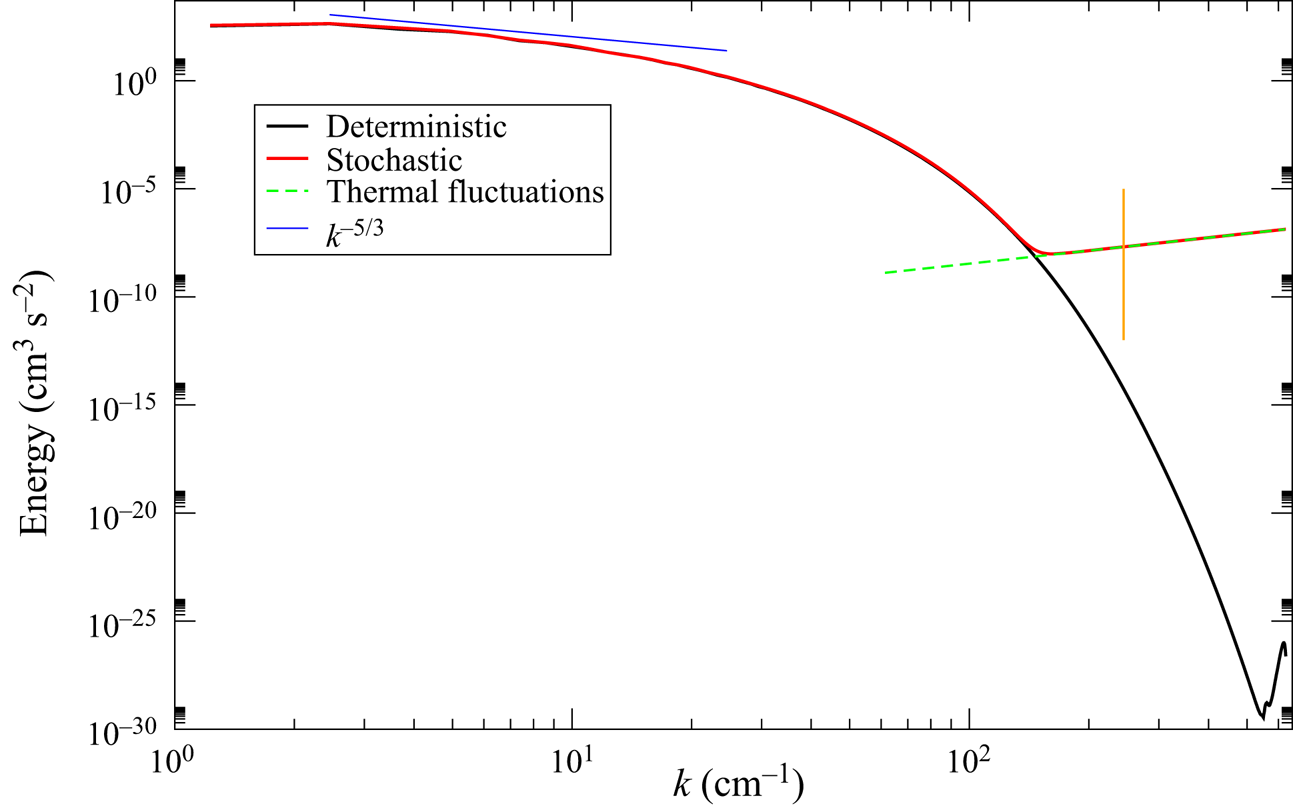
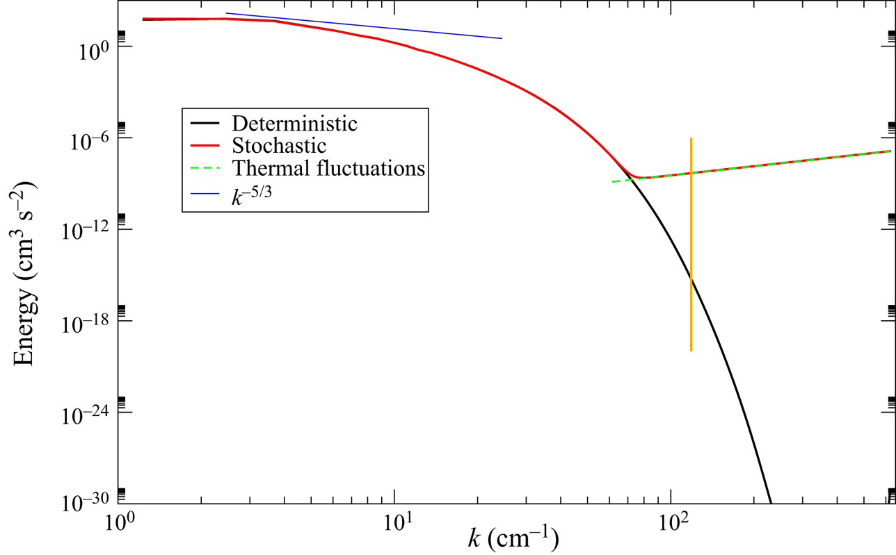
Spectra from Case 1 simulations, with and without thermal noise, roughly  $18\tau _{\eta }$ after restart are shown in figure 1 (compare with figure 1 in Eyink et al. Reference Eyink, Bandak, Goldenfeld and Mailybaev2021). We note that the behaviour of the deterministic spectrum at very high
 $k$ reflects limitations in the accuracy of double precision. We emphasize that the green dashed line in the figure corresponds to the theoretical spectrum of the fluctuations given by (2.10). Spectra from Case 2 simulations, with and without thermal noise, roughly
 $4\tau _{\eta }$ after restart are shown in figure 2. In both cases, the crossover between the turbulence spectrum and the thermal fluctuation spectrum occurs at
 $k \approx \frac 12 k_{\eta }$, in agreement with the estimate given by
 $k_{\theta }$.
Specific energy density spectrum for Case 1, with (red) and without (black) thermal noise. The blue line is the  $-5/3$ slope; the green line represents the spectrum of thermal fluctuations given by (2.10). The Kolmogorov wavenumber
 $k_{\eta } = 2{\rm \pi} /\eta \approx {251}\,\mathrm {cm}^{-1}$ is indicated by the vertical orange line. The uptick on the far right of the spectrum reflects loss of accuracy due to limitations of floating point accuracy.

Specific energy density spectrum for Case 2 (see figure 1 caption); here,  $k_{\eta } \approx {119}\,\mathrm {cm}^{-1}$. We note that values of the spectrum above 217 cm
 $^{-1}$ cannot be computed accurately because of limitations of double precision floating point, and are not shown here.

It is useful to define (Khurshid et al. Reference Khurshid, Donzis and Sreenivasan2018; Buaria & Sreenivasan Reference Buaria and Sreenivasan2020)
 \begin{equation} \phi( k ) \equiv \frac{{\rm d} (\ln E(k))}{{\rm d} (\ln k)} = \frac{k}{E}\,\frac{{\rm d}E}{{\rm d}k}, \end{equation}
given that, in the absence of thermal fluctuations, the energy spectrum in the dissipation range can be modelled as
 \begin{equation} E(k) = C (k \eta)^\alpha \exp( - \beta (k \eta)^\gamma ), \end{equation}
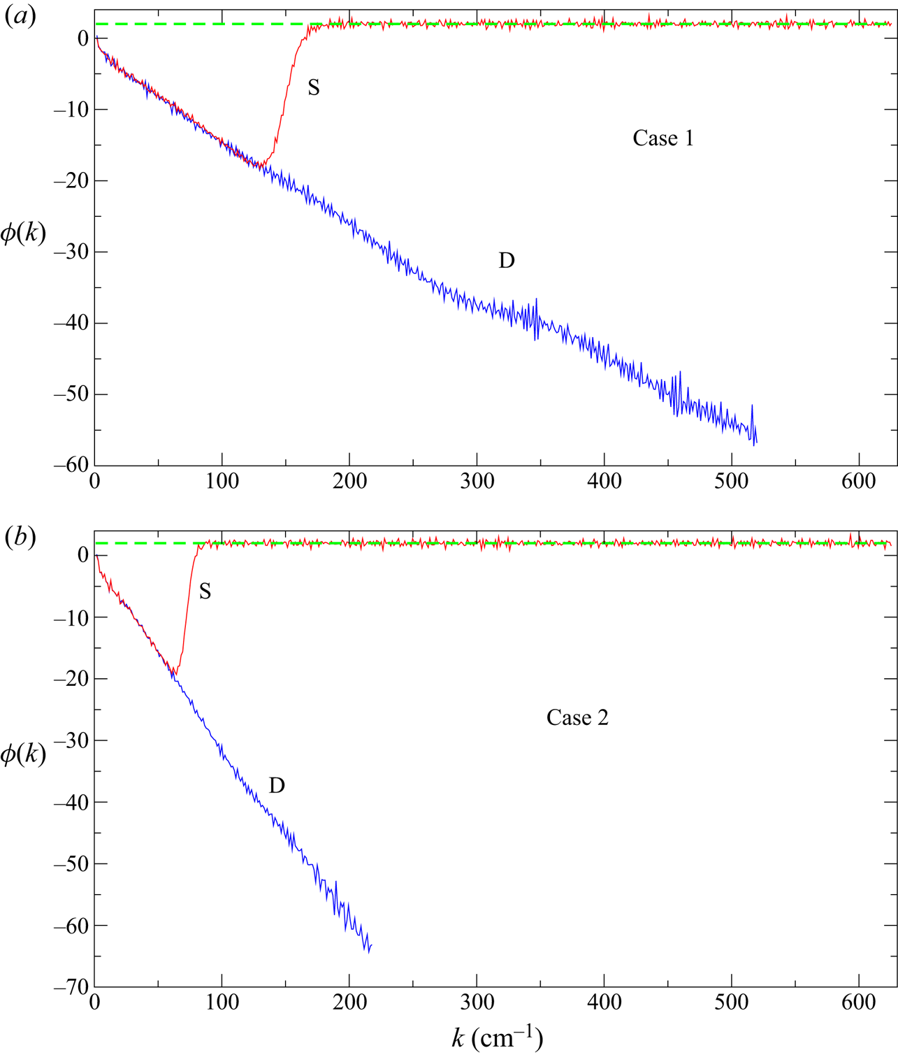
in which case we expect  $\phi ( k ) = \alpha - \beta \gamma (\eta k)^\gamma$. Figure 3 shows that the function
 $\phi (k)$ is approximately linear for
 $k \lessapprox 100\,\mathrm {cm}^{-1}$ in Case 1, and for
 $k \lessapprox 50\,\mathrm {cm}^{-1}$ in Case 2. Above these wavenumbers for the simulations with thermal fluctuations, the function rises rapidly, plateauing at
 $\phi (k) \approx 2$, as expected. For the deterministic runs, the compensated function
 $\tilde {\phi }(k) \equiv \phi (k)/(\gamma (k \eta )^\gamma )$ is approximately constant, with
 $\tilde {\phi } \approx {-6.5}$ and
 $-5.5$ for
 $\gamma \approx {0.9}$ and
 $0.95$ in Cases 1 and 2, respectively. The deterministic results for
 $\phi$ and
 $\tilde {\phi }$ are in reasonable agreement with those reported by Khurshid et al. (Reference Khurshid, Donzis and Sreenivasan2018) and Buaria & Sreenivasan (Reference Buaria and Sreenivasan2020), but the runs with thermal noise confirm the original insight of Betchov (Reference Betchov1957) that equipartition should occur at wavenumbers near the Kolmogorov scale.
Function  $\phi (k)$ for (a) Case 1 and (b) Case 2. The dashed line is
 $\phi = 2$. Labels S (stochastic) and D (deterministic) indicate simulations run with and without thermal fluctuations. Here, we have considered only the range of the spectrum where the values can be computed accurately in double precision.

We also measured the velocity derivative skewness and kurtosis as
 \begin{equation} \mathcal{S} ={-} \frac{\overline{u_{1,1}^3}}{(\overline{u_{1,1}^2})^{3/2}} \quad\mathrm{and}\quad \mathcal{K} = \frac{\overline{u_{1,1}^4}}{(\overline{u_{1,1}^2})^2}, \end{equation}
where
 \begin{equation} \overline{{u}_{i,j}^n} = \frac{1}{V} \int \mathrm{d}\boldsymbol{r}\,(u_{i,j}(\boldsymbol{r}))^n \quad\mathrm{and}\quad u_{i,j}(\boldsymbol{r}) = \frac{\partial u_i(\boldsymbol{r})}{\partial r_j}. \end{equation}
For homogeneous isotropic turbulence, one typically has  $\mathcal {S} \approx \frac 13- \frac 12$ and
 $\mathcal {K} \approx 4$. At thermodynamic equilibrium, we expect
 $\mathcal {S} = 0$ and
 $\mathcal {K} = 3$ since thermal fluctuations are Gaussian distributed; this was confirmed in simulations with no external forcing (not shown). In Case 1 (strong forcing), the measured skewness is
 $\mathcal {S} \approx {0.48}$ and the kurtosis is
 $\mathcal {K} \approx {4.3}$; in Case 2 (weak forcing),
 $\mathcal {S} \approx {0.45}$ and
 $\mathcal {K} \approx 4.1$. These values did not change significantly when the simulations were repeated with the thermal noise disabled (i.e. deterministic forced Navier–Stokes). As functions of time, the skewness and kurtosis are smooth but vary significantly. For example, kurtosis in Case 2 was as low as 3.7 and as high as 4.4.
While the skewness and kurtosis are little affected by thermal noise, Eyink et al. (Reference Eyink, Bandak, Goldenfeld and Mailybaev2021) have argued that the extreme intermittency in the far-dissipation range predicted by Kraichnan (Reference Kraichnan1967) is replaced by Gaussian thermal equipartition. As in previous numerical studies (Chen et al. Reference Chen, Doolen, Herring, Kraichnan, Orszag and She1993), this intermittency can be diagnosed by measuring the probability distribution functions (p.d.f.s) for various higher-order derivatives of the velocity, normalized using
 \begin{equation} \mathcal{L}_n(\boldsymbol{u}) = \frac{{(-\nabla^2})^n \boldsymbol{u}} {\left\langle\left( {(-\nabla^2})^n \boldsymbol{u} \right)^2 \right\rangle^{1/2}} \quad \mathrm{for} \ n=0,2,3,4, \end{equation}
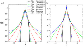
We evaluate the Laplacian using the finite difference operator used by the integration scheme as described in § 3. These p.d.f.s probe increasingly smaller scales for larger  $n$. In figure 4, we show numerical results for both deterministic and stochastic runs. In the absence of thermal fluctuations, the p.d.f.s for
 $n=2,3,4$ have stretched-exponential tails that grow broader with increasing
 $n$, as in Chen et al. (Reference Chen, Doolen, Herring, Kraichnan, Orszag and She1993). In the stochastic simulations, we see quite the opposite behaviour, with the p.d.f.s having suppressed tails for increasing
 $n$, and becoming nearly Gaussian for
 $n=3,4$ in Case 1 and
 $n=2,3,4$ in Case 2, with variances that match unforced simulations with noise. In the absence of large-scale external forcing, all three p.d.f.s are Gaussian (not shown) with variances that match theoretical predictions to within 7 %, as expected for thermal fluctuations at thermodynamic equilibrium. These results support the prediction of Eyink et al. (Reference Eyink, Bandak, Goldenfeld and Mailybaev2021).
P.d.f.s for  $\mathcal {L}_0$ (black),
 $\mathcal {L}_2$ (red),
 $\mathcal {L}_3$ (green) and
 $\mathcal {L}_4$ (blue) for deterministic (solid lines) and stochastic (dashed lines) simulations. (a) Strong forcing (Case 1); (b) weak forcing (Case 2). Note that in both panels, solid and dashed black curves overlap, and in (b), the green and blue dashed curves overlap.

5. Concluding remarks
It is generally assumed that the large separation between the scale at which turbulent eddies are strongly damped and the molecular mean free path implies that thermal fluctuations are irrelevant in turbulent flows. However, statistical mechanics tells us that thermal fluctuations are present at all wavelengths, and the fluctuation-dissipation theorem shows their close relation to viscous dissipation. Characterizing the impact of thermal fluctuations on turbulent flow requires the introduction of a dimensionless parameter,  $\theta _\eta$, related to temperature. For values of
 $\theta _\eta$ representative of flows of interest, the presumption that the viscous dissipation range is well-separated from the thermal range breaks down. The numerical simulation results in this paper confirm theoretical predictions (Betchov Reference Betchov1957; Eyink et al. Reference Eyink, Bandak, Goldenfeld and Mailybaev2021) that the thermal equipartition range in the energy spectrum can dominate in the dissipation range at length scales comparable to the Kolmogorov length. This means that to model sub-Kolmogorov-scale turbulence in this regime, the conventional incompressible Navier–Stokes equations must be augmented to include thermal fluctuations, as in the Landau–Lifschitz fluctuating Navier–Stokes equations. Particle simulations, such as direct simulation Monte Carlo, are also useful, and preliminary results (McMullen et al. Reference McMullen, Krygier, Torczynski and Gallis2021) also seem to confirm the importance of thermal fluctuations.
While these numerical results agree with theoretical estimates, experimental verification remains crucial but very challenging. Traditional techniques, such as hot-wire anemometry and particle imaging velocimetry, so far lack the resolution and sensitivity to be applicable at the sub-Kolmogorov scales of turbulent flows. Conceptually, it is not even clear that such methods based on continuum fluid descriptions suffice to measure molecular velocities coarse-grained over mesoscopic scales. It may be more practical to look for indirect evidence of the effects of thermal fluctuations in the dissipation range. For example, high-Schmidt/Prandtl-number scalar mixing, droplet and bubble formation, and chemical reactions are all known to depend strongly on sub-Kolmogorov scales, but can be equally influenced by thermal noise, so that the two effects may compete in determining observed rates and characteristics. For the case of high-Schmidt mixing, see Eyink & Jafari (Reference Eyink and Jafari2021).
Finally, in this work we focused on the dissipation range of fully-developed homogeneous turbulence but we expect thermal fluctuations to be important for other turbulent flow scenarios. For example, they may play an important role in triggering the transition to turbulence (Betchov Reference Betchov1961; Luchini Reference Luchini2017). Thermal fluctuations may also be crucial in the generation of unpredictability, leading to spontaneous stochasticity. In fact, thermal noise is expected to contribute for any fluid modes that are strongly affected by molecular dissipation, such as the viscous sublayer eddies of wall-bounded turbulence. For such scenarios and others, fluctuating hydrodynamics provides a powerful theoretical and numerical tool for future work.
Supplementary material
Supplementary material is available at https://doi.org/10.1017/jfm.2022.188.
Acknowledgements
The authors thank A. Donev, M. Gallis and J. Goodman for insightful discussions.
Funding
This work was supported by the US Department of Energy, Office of Science, Office of Advanced Scientific Computing Research, Applied Mathematics Program under contract no. DE-AC02-05CH11231 (J.B., A.N., A.G.). The work of G.E. was supported by the Simons Foundation Targeted Grant in MPS-663054. This research used resources of the National Energy Research Scientific Computing Center, a DOE Office of Science User Facility supported under Contract no. DE-AC02-05CH11231.
Declaration of interests
The authors report no conflict of interest.
Author contributions
All authors contributed equally to this paper.
Data availability statement
The code/data that support the findings of this study are openly available in the github repository https://github.com/AMReX-FHD/FHDeX.