1 Introduction
Many recent papers in political science and economics study rainfall and its relationship to important political factors, such as civil conflict, economic shocks, protest, and elections (Miguel, Satyanath, and Sergenti Reference Miguel, Satyanath and Sergenti2004; Brückner and Ciccone Reference Brückner and Ciccone2011; Hsiang, Meng, and Cane Reference Hsiang, Meng and Cane2011; Hsiang, Burke, and Miguel Reference Hsiang, Burke and Miguel2013; Chen Reference Chen2013; Madestam et al. Reference Madestam, Shoag, Veuger and Yanagizawa-Drott2013; Dell, Jones, and Olken Reference Dell, Jones and Olken2014). In the study of American politics, the relationship between rainfall and voting dates back to 1925, when the rise of populism was attributed to drought (Barnhart Reference Barnhart1925). More recently, Gomez, Hansford, and Krause (Reference Gomez, Hansford and Krause2007) focus on the relationship between rainfall and voter turnout.Footnote 1
In addition to being important for substantive reasons, rainfall is often seen as a clever measurement strategy to introduce randomness into what is otherwise a complicated and interrelated world. The underlying assumptions in prominent works are that “election day rainfall is the best available instrument for turnout because it (1) has sufficient explanatory power to identify the IV model and (2) is clearly exogenous to electoral outcomes” (Gomez and Hansford Reference Gomez and Hansford2010, note 26) and that “it is intuitively plausible that the rainfall instruments are exogenous” (Miguel, Satyanath, and Sergenti Reference Miguel, Satyanath and Sergenti2004, p. 745).
Still, assignment of weather at the county level is highly correlated in space. If San Francisco receives a high rainfall shock on election day, it is very likely that nearby San Jose will also receive high rainfall. Nearby counties are likely to receive similar amounts of rainfall, but it is challenging to define the extent of clustering. Even if we consider the San Francisco Bay Area to be a cluster, all counties in the cluster will not be assigned to exactly the same treatment. Weather patterns do not follow political boundaries, and estimating the variance around point estimates is complicated by clustered assignment where cluster boundaries are undefined.
In this analysis, I propose a new technique to improve inference of political relationships involving climate data. I use randomization inference for variance estimation of the effect of clustered rainfall shocks on political outcomes.Footnote 2 To create a sampling distribution under the sharp null hypothesis of no effect, I estimate average treatment effects (ATEs) under other potential randomizations using draws from historical rainfall data.
I permute the weather assignments and regenerate the regression estimates for each election year in a pooled regression. Each election year is tested against a random draw from 73 years of historic rainfall data on election or would-be election days. I conduct the RI procedure using five different assumptions of unit independence. Two specifications use political units and assume independence at the county and state levels, and two specifications use boundaries from the National Weather Service and assume independence at the county warning area (CWA) and region levels. My preferred specification to create the sampling distribution draws potential randomizations from the national distribution of rainfall across all counties in a particular year.
I demonstrate that specifications assuming independent assignment by county or clustered randomization by state or other sub-national unit likely underestimate the variance of point estimates. I replicate the paper by Gomez, Hansford, and Krause (Reference Gomez, Hansford and Krause2007) on rainfall and voter turnout in the United States and apply my proposed inference strategy. In addition to using rainfall levels, I calculate standardized indices with two methods. I use standardized indices so that the rainfall treatment is a shock that is relative to that county’s typical conditions.
I find that the sampling variability around the point estimate identified by the authors is much greater when taking into account that weather treatments are clustered. When I assume that counties are independent, the
 $p$
-value remains
 ${<}0.001$
for rainfall levels and indices. However, when I assume that weather treatments are correlated across the country, the
 $p$
-values increase to 0.084 for rainfall (inches), 0.405 for the rainfall index (z-score), and 0.314 for the rainfall Standardized Precipitation Index (SPI).
My results highlight the weaknesses of standard tests of statistical significance when scholars ignore the complicated clustering of random assignment in climate and other spatially correlated data. The cross-cluster correlations across counties, states, and even large weather regions violate the assumption required for cluster-robust standard errors, where correlation is allowed within clusters but not across them. Other variance estimation methods use spatial-robust variance matrix estimators that allow correlations to decay with spatial distances, but they introduce another level of modeling assumptions in order to specify the matrix.
With randomization inference, researchers can be agnostic about complex clustering across units, since national draws of potential randomizations will preserve patterns of dependence and independence across counties. By using permutations of out-of-sample weather patterns and creating a sampling distribution of the coefficient estimates under the sharp null hypothesis, it is a non-parametric approach that does not rely on distributional assumptions.
My technique is widely applicable when analyzing spatially clustered climate variables, which are increasingly used as explanatory and instrumental variables for a wide range of outcomes. Rainfall has been used as an explanatory variable to study conflict, income, health, and education (Maccini and Yang Reference Maccini and Yang2009; Hsiang, Meng, and Cane Reference Hsiang, Meng and Cane2011; Hsiang, Burke, and Miguel Reference Hsiang, Burke and Miguel2013) and as an instrumental variable to study the effects of protest participation on voting (Madestam et al. Reference Madestam, Shoag, Veuger and Yanagizawa-Drott2013) and the effects of income shocks on civil conflict and democratization (Miguel, Satyanath, and Sergenti Reference Miguel, Satyanath and Sergenti2004; Brückner and Ciccone Reference Brückner and Ciccone2011).Footnote 3 My method relies on out-of-sample data that are easily accessible for climate variables, and it can be used with cross-sectional and panel models.
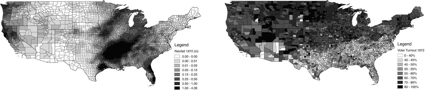
Election Day Rainfall Amounts and Voter Turnout by County (1972).

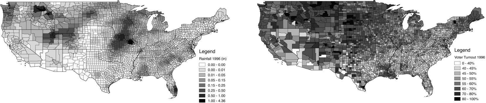
Election Day Rainfall Amounts and Voter Turnout by County (1996). Note: Rainfall amounts on presidential election days (November 7, 1972 and November 5, 1996) calculated by author using Kriging spatial interpolation from 12 nearest weather stations. See Appendix for data source and processing details. Voter Turnout data from Gomez, Hansford, and Krause (Reference Gomez, Hansford and Krause2015).

2 Randomization Inference with Clustered Rainfall
2.1 Clustered treatment assignment
To understand the assumptions inherent in treating rainfall as random, I propose a thought experiment. In the simplest example, the researcher would treat each county in the United States as an independent observation and distribute rainfall shocks with simple random assignment. The researcher would randomly assign amounts of rainfall to each county on each day, with each county’s rain being independent of its neighbors’ rain. However, rainfall is correlated across neighboring counties, as can be seen in Figures 1 and 2. The researcher instead needs to distribute rainfall shocks with clustered assignment.
In the next example, we can relax the assumption of randomization by county and instead consider states as the unit of cluster assignment, where each state’s treatment assignment is independent of a neighboring state’s treatment assignment. In a standard experimental framework, all counties in a state would be assigned to treatment or to control. However, on a given day, counties within states receive different amounts of rainfall and different deviations from their historical average rainfall. We could instead allow counties’ treatment assignments to be independent across states but correlated within the state, which is the assumption used for cluster-robust standard errors at the state level. Unfortunately, this is still problematic because it assumes that neighboring counties on opposite sides of a state line have unrelated treatment assignments.
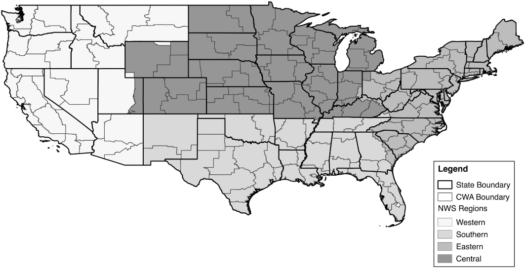
Next, since political boundaries are unlikely to reflect weather patterns, we can use boundaries defined by the National Weather Service for CWAs (115 primary areas within the contiguous United States) and regions (four within the contiguous United States) shown in Figure 3 (NWS 2009, 2012, 2016). County warning areas (CWAs) are much smaller than states, and neighboring CWAs have highly correlated rainfall measures. Even the large regions encounter correlation in rainfall between counties on opposite sides of regional borders. These examples highlight the challenge of accounting for clustered treatment assignment when the treatments do not adhere to well-defined units.
National Weather Service Regions and County Warning Areas. Note: There are 115 county warning areas in the contiguous United States. County Warning and Forecast Areas are designated by counties/parishes (or parts thereof), and independent cities surrounding a Weather Forecast Office. Details and shapefiles for CWAs and NWS Regions are available on the National Weather Service website (NWS 2009, 2012, 2016).

Accounting for clustered treatment assignment can be complicated, and standard techniques rely on many assumptions about the specific nature of clustering. OLS requires that disturbances are identical and independently distributed (i.i.d.) in order to estimate consistent standard errors. When observations are correlated, this estimation strategy is apt to underestimate the true variance in the point estimates.
Researchers in political science and economics working with weather data often use clustered standard errors to account for clustered treatment assignment (Miguel, Satyanath, and Sergenti Reference Miguel, Satyanath and Sergenti2004). Still, estimating cluster-robust standard errors in OLS requires the assumption that there is correlation within clusters but not across them, and states and even large weather regions violate this assumption.Footnote 4 Other scholars have described different sandwich-type robust standard errors and covariance matrix estimators that can accommodate more complicated clustering structures (Conley Reference Conley1999; Aronow, Samii, and Assenova Reference Aronow, Samii and Assenova2015; Cameron and Miller Reference Cameron and Miller2015), but they also rely on modeling assumptions to estimate that structure.
2.2 Randomization inference
Instead, I suggest using randomization inference to test the sharp null hypothesis of no effect and estimate the uncertainty around the point estimates (Fisher Reference Fisher1935; Rubin Reference Rubin1990; Erikson, Pinto, and Rader Reference Erikson, Pinto and Rader2010, Reference Erikson, Pinto and Rader2014). The estimated ATE from the observed rainfall pattern is compared to a sampling distribution of estimated ATEs under the sharp null hypothesis of no effect (Gerber and Green Reference Gerber and Green2012, p.62).
In the observed dataset of presidential election days, each county–year observation reveals only one of its potential outcomes: the treated potential outcome if it has high rainfall and the untreated potential outcome if it does not. If the sharp null hypothesis of no effect were true (i.e. if high rainfall has no effect on voter turnout for any observation) then each county–year observation reveals both potential outcomes because they are equal. These outcomes can then be tested against other potential randomizations to create a sampling distribution of estimated ATEs under the sharp null hypothesis.
For example, in 1948 all counties received a certain rainfall treatment assignment and revealed their potential voter turnout outcomes. King County in Washington, where Seattle is located, received almost half an inch of rain, which is 0.12 standard deviations above average. It therefore revealed its treated potential voter turnout outcome of 61%. If the sharp null hypothesis of no effect were true, then voter turnout would still have been 61% if it were a sunny day.
I use historical county-level data to obtain potential clustered assignments of rainfall shocks for each county. With 73 years of county-level rainfall data for election and would-be election days from 1940 to 2012, I have a wide range of possible random assignments that incorporate the clustered treatment assignment of rainfall.Footnote 5 Using historical data of actual weather patterns eliminates the need to simulate weather patterns or make assumptions about unit boundaries for clustering.
I calculate p-values for the estimated ATE of rainfall on voter turnout with null sampling distributions that use five different assumptions of the randomization procedure for counties. The assumptions are that counties are 1) independent, 2) correlated within CWAs, 3) correlated within states, 4) correlated within weather regions, and 5) correlated across the United States.
In the most liberal assumption, I assume that randomization is done by county–year. For example, a potential assignment of rainfall for county 1A in state 1 is a random draw from county 1A’s rainfall from 1940 to 2012. The potential assignment for its neighboring county 1B is completely independent.
A more conservative approach assumes that counties are correlated within states within a year, such that randomization is done by state–year. To create a set of potential weather patterns from which to create the null sampling distribution, the potential assignment of rainfall for all counties within state 1 is a random draw from state 1’s rainfall data on election and would-be election days from 1940 to 2012. In this case, all counties within state 1 will have rainfall from the same year. However, the potential assignment for all counties in neighboring state 2 will be independent and could be drawn from a different year.
The most conservative approach assumes that rainfall assignments on would-be election days for each county are correlated across the country and are not restricted by state lines. In this case, I assign each presidential election to a randomly selected weather pattern, where all counties are assigned to the same year. For example, I simulate the distribution of estimated ATEs under the sharp null hypothesis for the 1948 presidential election by randomly sampling with replacement from all 73 years of weather data (including 1948) to obtain a possible randomization. I then continue drawing different yearly rainfall distributions to fill out the sampling distribution of estimated ATEs.Footnote 6
The estimation of p-values from null sampling distributions based on county–year, CWA–year, state–year, and region–year randomizations serve as falsification tests. When I use the US–year randomization, the random draws of national weather patterns will preserve whatever spatial correlation exists across the country. Where counties are independent, it will preserve this independence. Where counties are correlated, it will preserve these correlations. Therefore, if all county, CWA, state, and region rainfall measures are in fact independent across cluster units, then the p-values estimated by the respective RI method will be equivalent to the US–year RI method.
If the p-values are the same under all five assumptions, then we can consider counties to be independent. However, I expect that sampling distributions will be narrower and the p-values will be much smaller when counties and states are assumed to be independent, which would highlight the overconfidence around point estimates when clustered treatment assignment is not addressed.
3 Results
In this paper, I extend the work by Gomez, Hansford, and Krause (Reference Gomez, Hansford and Krause2007) on voter turnout during 14 presidential elections from 1948 to 2000 in 3,115 counties.Footnote 7 Their analysis uses a linear cross-sectional random effects regression model to estimate the relationship between county-level rainfall and voter turnout during US presidential elections.
The main rainfall treatment results that Gomez, Hansford, and Krause (Reference Gomez, Hansford and Krause2007) present are based on the absolute amount of rainfall in each county–year (inches) or the deviation from each county’s average from 1948 to 2000 (inches). In each case, rainfall is presented as a continuous treatment variable. I begin by replicating their findings using rainfall in inches. I continue with the same model but with standardized indices for rainfall representing deviations from historical average by county.
In addition to using rainfall levels, I calculate standardized indices with two methods. I use a standardized index so that the rainfall treatment is a shock that is relative to that county’s typical conditions. This approach relaxes the assumption that one inch of rainfall has the same effect in every county. The motivating theory is that relatively high rainfall would affect the cost of voting by influencing voters’ travel to the polling station. However, counties have different mean levels of rainfall and have adapted to different circumstances. For example, an inch of rainfall on election day in San Diego, CA would be a very different substantive shock than one inch of rainfall in Seattle, WA. Since voters adapt to their environment and infrastructure systems vary in their ability to handle weather events, I believe that a deviation from average is a more appropriate test of the theory. Recent papers in political science and economics using rainfall data have also highlighted the theoretical weakness of using levels and instead recommend standardized indices (Koubi et al. Reference Koubi, Bernauer, Kalbhenn and Spilker2012; Hsiang, Burke, and Miguel Reference Hsiang, Burke and Miguel2013; Dell, Jones, and Olken Reference Dell, Jones and Olken2014).
The first index is a simple standardized index where the rainfall measure is a z-score. The rainfall level is transformed by subtracting the county’s historical mean and dividing by the standard deviation. While this index is intuitively simple, the climate science literature argues that precipitation data tends not to be normally distributed. Rather the index is skewed to the right and the infrequent days of high rainfall create outliers. For the second index, I follow many climate scientists and calculate an SPI based on the empirical cumulative distribution function (ECDF).Footnote 8
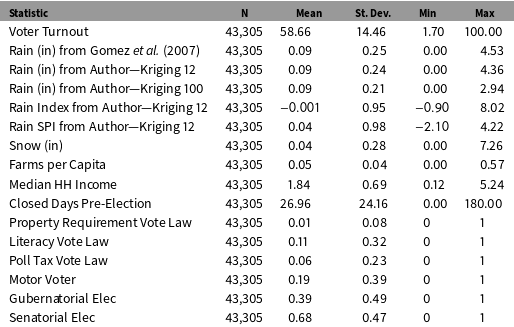
I use data collected by Gomez, Hansford, and Krause (Reference Gomez, Hansford and Krause2007) and provided in a replication package (Gomez, Hansford, and Krause Reference Gomez, Hansford and Krause2015). Their paper provides details on the data sources and measurement of the outcome and covariates. I perform my own spatial interpolation of the rainfall data in order to calculate historical rainfall by county on all would-be election days from 1940 to 2012.Footnote 9 I use the same weather station source as the prior authors, but I have slightly different estimates for rainfall amounts on election days.Footnote 10 Summary statistics are provided in Table 1, and the Appendix includes details on the data sources and spatial interpolation.
Summary Statistics.

Note: Summary statistics of variables from replication package provided by Gomez, Hansford, and Krause (Reference Gomez, Hansford and Krause2007). See original paper for details on the data sources and measurement of the outcome and covariates. I perform Kriging spatial interpolation on weather station rainfall data using 12 or 100 nearest stations in order to calculate historical rainfall by county on would-be election days from 1940 to 2012. My sample is smaller than Gomez, Hansford, and Krause (Reference Gomez, Hansford and Krause2007) by 35 observations since I used county lines from 2000 to estimate county mean rainfall levels, and seven counties had been redistricted and no longer existed. See Appendix for details.
3.1 Replication
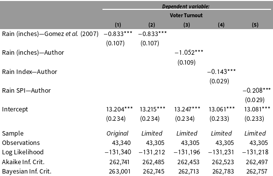
In Table 2, I replicate the findings by Gomez, Hansford, and Krause (Reference Gomez, Hansford and Krause2007) of the relationship between rainfall inches and voter turnout.Footnote
11
Column 1 replicates the findings from their main estimator,Footnote
12
which uses a maximum-likelihood model with random effects for each county, fixed effects for each year, and conventional standard errors. Column 2 shows that the estimate with rainfall data from Gomez, Hansford, and Krause (Reference Gomez, Hansford and Krause2007) does not change when I exclude the seven counties not in my data set due to redistricting. Column 3 uses rainfall data that I processed, which creates a point estimate of larger magnitude with a coefficient on rainfall (inches) of
 $-1.052$
instead of Gomez, Hansford, and Krause (Reference Gomez, Hansford and Krause2007)’s coefficient of
 $-0.833$
.
Replication of Main Findings in Gomez, Hansford, and Krause (Reference Gomez, Hansford and Krause2007) with Additional Rainfall Data Sources and Measurement.

 $^{\ast }p<0.1$
;
 $^{\ast \ast }p<0.05$
;
 $^{\ast \ast \ast }p<0.01$
. Note: Table replicates the findings from Gomez, Hansford, and Krause (Reference Gomez, Hansford and Krause2007) using a maximum-likelihood linear cross-sectional random effects model (CSRE) with random effects for each county, fixed effects for each year, and conventional standard errors. Covariates omitted from table (see Appendix for coefficients). Columns 1 and 2 use data from Gomez, Hansford, and Krause (Reference Gomez, Hansford and Krause2015) replication package of rainfall in inches. Column 1 reflects the full dataset from Gomez, Hansford, and Krause (Reference Gomez, Hansford and Krause2007), and Columns 2–5 reflect a dataset with 35 fewer observations due to seven counties not being present when calculating rainfall using county lines from 2000. Columns 3–5 use rainfall data processed by the author in inches and as indices relative to the county’s historical mean. Column 4 uses a rainfall index calculated using a z-score, and Column 5 uses a Standardized Precipitation Index based on the empirical cumulative distribution function.
The estimated ATE of
 $-1.05$
in Table 2, Column 3 signifies that a county that receives one inch of rainfall on election day is likely to have approximately 1 percentage point lower voter turnout. The mean voter turnout in the sample was
 $59\%$
. However, the use of rainfall levels does not take into account that counties have different mean levels of rainfall and that one inch of rain represents a different shock in different places.
To assess the impact of a rainfall shock, I use indices that normalize rainfall within each county instead of using rainfall levels. Column 4 uses a z-score to measure rainfall shocks that is calculated by subtracting that county’s historical mean rainfall on election days or would-be election days from 1940 to 2012 and dividing by its standard deviation. The estimated coefficient on this rainfall index is
 $-0.143$
. Still, this estimate is sensitive to outliers, because rainfall data are skewed right and each county tends to have a few high rainfall days during the sample that generate very high index values.
Column 5 uses my preferred specification of an SPI that reduces the extremity of outliers. It has an estimated coefficient on the rainfall index of
 $-0.208$
. A one unit change in the index signifies one standard deviation higher rainfall compared to the county’s historical mean. The substantive interpretation is that one standard deviation higher rainfall is associated with
 $0.208$
percentage point lower voter turnout. Each specification is statistically significant at
 $p<0.01$
using conventional standard errors.
3.2 Randomization inference
I extract the estimated ATEs for rainfall inches and index from Columns 3–5 in Table 2 and test the sharp null hypothesis of no effect to make inferences about the uncertainty around these estimates. The estimated ATEs for the rainfall level and rainfall indices are compared to null sampling distributions where potential randomizations are drawn using different assumptions about the treatment assignment procedure.
Randomization Inference Estimates of ATE Variance Under Different Assumptions.

Note: Table draws estimated ATEs from Columns 3–5 in Table 2. Two-tailed p-values are estimated with randomization inference from sampling distributions of 1000 estimated ATEs under the sharp null hypothesis of no effect using five different assumptions of the clustered randomization procedure. Potential randomizations are drawn from county-level rainfall on each election day or potential election day from 1940 to 2012. The first row uses rainfall (in), the second row uses a z-score index, and the third row uses a Standardized Precipitation Index. County assignment assumes that each county is independent and supposes simple random assignment at the county level. County warning area (CWA) and region are National Weather Service classifications. For CWA, state, and region specifications, I assume that treatment assignment is clustered within that unit in a given year but each unit is independent of other units. US assignment assumes that treatment assignment is clustered within the entire United States in a given year.
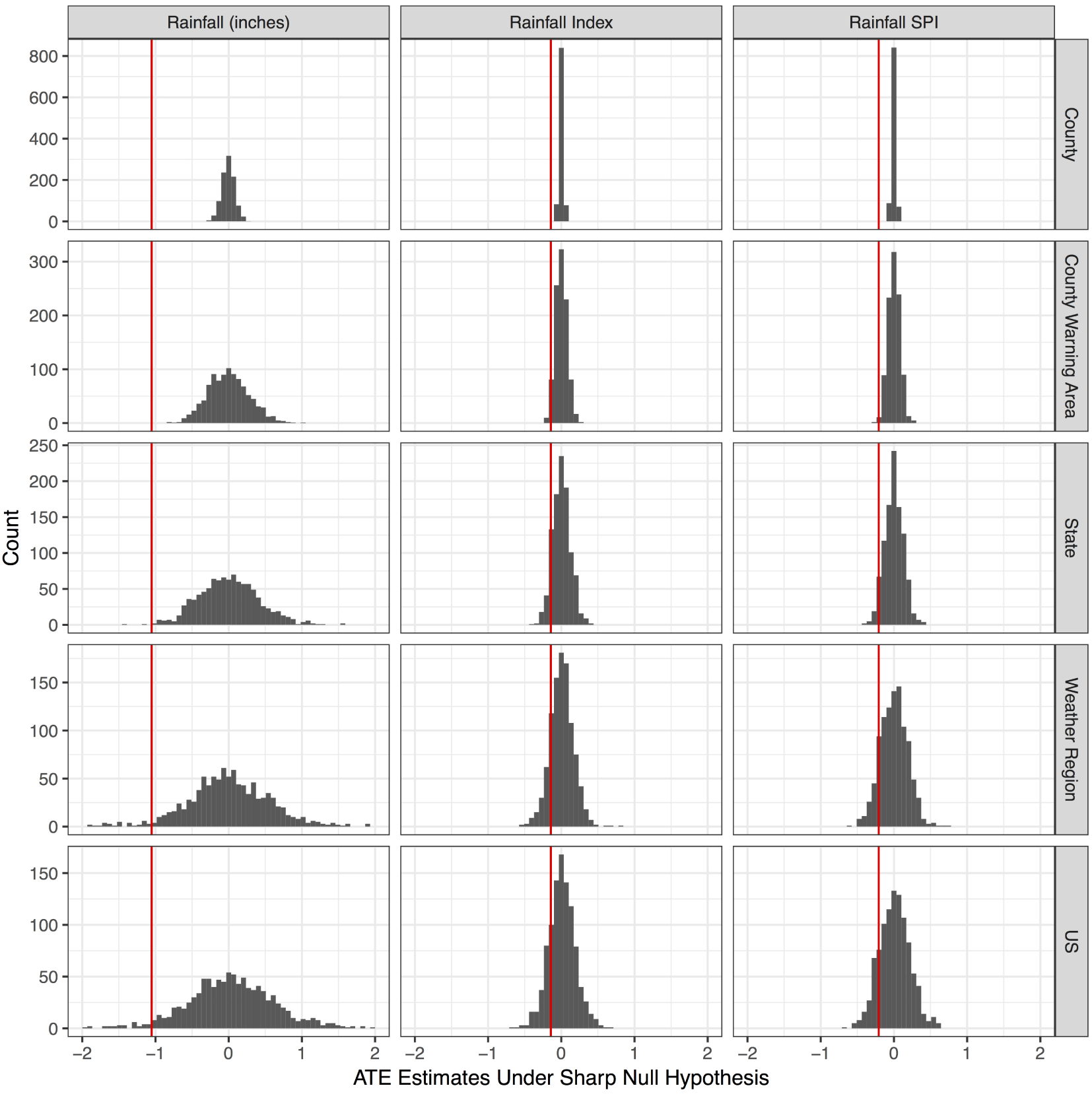
The p-values calculated using randomization inference are presented in Table 3. The sampling distributions using different rainfall measures and randomization assumptions are shown in Figure 4, where the vertical line represents the observed ATE for that specification.
Sampling Distribution of ATE Estimates for Rainfall by Measurement and Cluster Unit. Note: Figure represents sampling distributions of estimated ATEs under the sharp null hypothesis of no effect. Potential randomizations are random draws from county-level rainfall data from 1940 to 2012 on election or potential election days. Differences in measurement are reflected in each column. The first column uses rainfall (in), the second column uses a z-score index, and the third column uses a Standardized Precipitation Index. The dotted lines represent the estimated ATEs of
 $-1.052$
for rainfall (in),
 $-0.143$
for rainfall index, and
 $-0.208$
for rainfall SPI from Table 2. Different assumptions about the cluster unit are reflected in each row. County assignment assumes that each county is independent and supposes simple random assignment at the county level. County warning area (CWA) and region are National Weather Service classifications. For CWA, state, and region specifications, I assume that treatment assignment is clustered within that unit in a given year but each unit is independent of other units. US assignment assumes that treatment assignment is clustered within the entire United States in a given year. Figures use 1000 simulations each.

The estimated ATEs of rainfall on turnout appear to be very precisely estimated when using conventional OLS standard errors, as shown in Table 2. They are also far outside the narrow sampling distributions under the sharp null hypothesis of no effect when assuming that counties are independent, as shown in the top row of Figure 4, leading to p-values of
 ${<}0.001$
.
However, once clustered treatment assignment is taken into account, the sampling distributions become much wider. If we assume that counties are correlated within states but that states are independent of each other when creating the randomizations for the sampling distribution, the p-value is
 $0.014$
for rainfall (in) but increases to
 $0.237$
for the rainfall index and
 $0.102$
for the rainfall SPI.
Since weather patterns do not adhere to political boundaries, I also use National Weather Service boundaries. There are 115 CWAs in the contiguous United States, which are small groups of counties with similar weather patterns that cross state lines. The RI p-values for the CWA specification fall between the county and state level. There are four regions in the contiguous United States, and they are large groups of counties with similar weather patterns that also cross state lines in some areas. The RI p-values for the region specification fall between the state and national levels.
The last specification draws data for all counties within the same year when creating the potential randomizations for the sampling distribution. The p-values increase to
 $0.084$
for rainfall (in),
 $0.405$
for the rainfall index, and
 $0.314$
for the rainfall SPI.
The large changes in p-values across the five assumptions about the randomization procedure (county–year, CWA–year, state–year, weather region–year, and US–year) demonstrate that researchers are susceptible to drawing misleading inferences about the variance of the ATE when they ignore that weather treatments are clustered. These findings indicate that a rainfall shock has a more uncertain effect on voter turnout than previously thought.
4 Conclusion
Many scholars take advantage of the random timing of rainfall shocks to estimate the effects of rainfall on voter turnout or civil conflict, but estimating the variance of these effects is complicated. Rainfall shocks are arguably randomly assigned within a location over time, but random assignment occurs in clusters formed by weather patterns. In addition, these clusters are not clearly defined, and the correlations of weather patterns across counties are continuous over space and across political boundaries.
The principal contribution of this paper is the use of historical climate data to create sampling distributions in randomization inference, which preserve the clustered nature of rainfall shocks without the need to define units or model the correlations between counties. I use randomization inference to estimate the variance of the ATE of rainfall on voter turnout, and the sampling distribution of estimated ATEs under the sharp null hypothesis is based on random draws from historical rainfall distributions. I demonstrate that if scholars assume that random assignment is independent at the county or state levels, they will underestimate true variance. When I allow random assignment to be correlated across counties and states, the estimated variance around the rainfall effect is much larger than when using conventional OLS standard errors.
This technique is applicable to any research design where historical data are available and clustered assignments do not fit within clear boundaries, particularly natural experiments or those based on climate shocks. I provide a technique for randomization inference that is applicable when the treatment process is repeated over time and when there is available data for treatment assignments outside the confines of the primary dataset. In this paper, the primary dataset studied presidential election days, and historical data exist for would-be election days that are not included in the dataset of political outcomes.
Access to decades of global data makes this technique possible for data sources in areas as diverse as weather, socioeconomics, public health, and violence. Weather indicators and natural hazards, such as precipitation, temperature, wind, air particulates from fire or volcanic eruptions, and disasters such as tornadoes or hurricanes (Borden and Cutter Reference Borden and Cutter2008), are spatially clustered. Spatial autocorrelation patterns have also been documented in panel data on public health risks and disease transmission such as influenza (Malcolm Reference Malcolm2013), unemployment (Conley and Topa Reference Conley and Topa2002), and patterns of violence and criminology (Taylor and Covington Reference Taylor and Covington1988; Schutte and Weidmann Reference Schutte and Weidmann2011). Violence in civil conflict is often spatially clustered, and the specific location of violence in any given year has been argued to be indiscriminate or as-if random (Lyall Reference Lyall2009).
Weather shocks provide a clever way for researchers to make causal inferences about complicated political phenomena, but they come with the challenge of being a clustered treatment without clear boundaries. I provide an example of the overconfidence that comes from different assumptions about the clustering procedure, and I propose a fairly simple solution. If researchers are processing weather data and calculating the treatment within each unit, they can easily repeat this across many decades.
Supplementary material
For supplementary material accompanying this paper, please visit https://doi.org/10.1017/pan.2017.17.