1. INTRODUCTION
The introduction of the robust design by Taguchi (Reference Taguchi1991), or the so-called Taguchi method, has become a powerful tool for producing high-quality products at low cost. In this method (Belavendram, Reference Belavendram1995), a fractional factorial designs, or the so-called orthogonal arrays (OAs), are usually utilized to reduce the number of experiments under permissive reliability. The columns of the OA represent process/product parameters to be studied, whereas the rows denote the individual experiments, where each row contains the combination of factor levels at which an experiment is conducted. The signal–noise (S/N) ratio is then employed to decide the optimal factor levels. The Taguchi method has been widely accepted for robust design in many business applications. Nevertheless, most of the published research on the application of Taguchi method, such as Yang (Reference Yang2001), Tsao and Hocheng (Reference Tsao and Hocheng2002), and Li et al. (Reference Li, Al-Refaie and Yang2008), have been conducted to optimize one quality response of a process or product.
Typically, the quality response is divided into three main types: the smaller the better (STB), the nominal the best (NTB), and the larger the better (LTB) type response. In reality, most products are manufactured with more than one quality response of main concern. Therefore, the optimization of the multiresponse problem in the Taguchi method has received increasing attention over the past few years. For example, Phadke (Reference Phadke1989) optimized multiresponses individually. Then, a trade-off between quality loss and productivity by engineering judgment was used to decide the optimal factor levels for multiresponse problem. Unfortunately, this approach increases uncertainty in the decision-making process. Tai et al. (Reference Tai, Chen and Wu1992) assigned a weight to S/N ratio of each response. The S/N ratios for all responses were then combined into a single performance index by which the optimal factor levels were decided. Tong et al. (Reference Tong, Su and Wang1997) calculated the sum of the weighted-normalized quality losses for all responses. The multiresponse S/N ratio was then used to decide the optimal factor levels. In reality, it still remains difficult to determine and define a weight for each response. Pignatello (Reference Pignatello1993) discussed a manufacturing process with five responses. Then, regression technique-based approaches were utilized to determine tentative optimal factor levels. Reddy et al. (Reference Reddy, Nishina and Subash Babu1997) also employed regression technique-based approaches during unifying goal programming and the Taguchi method to optimize multiresponses simultaneously. However, regression approaches increase the complexity of the computational process. Thereafter, Su and Tong (Reference Su and Tong1997) and Antony (Reference Antony2000) utilized PCA to transform original responses into a set of uncorrelated principal components to choose the principal component, whose eigen value is greater than 1, as a multiresponse performance index by which the optimal factor levels for the multiresponse problem were determined. Nevertheless, when more than one principal component is selected, how to trade off to select a feasible solution is unknown. Jeyapaul et al. (Reference Jeyapaul, Shahabudeen and Krishnaiah2006) utilized a genetic algorithm (GA) with the Taguchi method for determining a weight for the S/N ratio of each response variable. Then, the sum of the weighted S/N ratios was used to decide optimal factor levels. The GA, however, is a search heuristic that provides near-optimal solutions for complex search spaces, such as production scheduling and transportations problems.
DEA (Charnes et al., Reference Charnes, Cooper and Rhodes1978, Reference Charnes, Cooper, Letwin and Seiford1994) has been widely used for measuring the performance of a group of DMUs with multiple inputs and multiple outputs at the organizational level, such as universities, hospitals, and banks. In contrast with the Taguchi method and some other approaches in the literature, DEA combines various inputs and outputs for a DMU into one performance measure, or relative efficiency, incorporates no a priori information about the response weights or importance, and avoids the intervention of the expert knowledge that increases uncertainty in the decision-making process. This research thus proposes and implements a procedure for solving the multiresponse problem in the Taguchi method using DEA approaches. This paper is organized as follows. Section 2 introduces DEA approaches. Section 3 presents the proposed procedure. Section 4 provides three illustrative case studies. Section 5 summarizes research results. Finally, conclusions are made in Section 6.
2. DATA ENVELOPMENT ANALYSIS
Generally, DEA is a fractional mathematical programming technique for evaluating the compared homogeneous MDUs with multiple inputs and multiple outputs. The most widely used DEA approach is the CCR model, which was developed by Charnes et al. (Reference Charnes, Cooper and Rhodes1978). Assume there are n DMUs each with m inputs and s outputs to be evaluated. The CCR model then measures the relative efficiency of each DMU once by comparing it to a group of the other DMUs that have the same set of inputs and outputs. Hence, there are n optimizations needed in the evaluation of performance for all DMUs. Let the DMU to be individually evaluated on any trial be designated as DMUo. Let the input and output vectors for DMUo be denoted by x io (i = 1, … , m) and y ro (r = 1, … , s), respectively. Let u r and v i be the virtual weights for the rth output and ith input, respectively. Let E o (= max θ) represent the relative efficiency of DMUo, where θ is a scalar. Then, E o can be estimated by solving the following mathematical model:

subject to
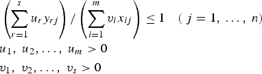
In the CCR model, the objective function is to maximize the sum of the weighted outputs relative to the sum of the weighted inputs for DMUo. The first constraint ensures that E j lies between 0 and 1 for all the n DMUs. The last two constraints are set to obtain nonnegative optimal u r and v i values; or u r* and v i*, respectively. Finally, DMUo is identified as efficient if the relative efficiency E o equals 1. Otherwise, DMUo is considered as inefficient. Similarly, the remaining (n − 1) DMUs are measured.
Few researchers have used the CCR model for solving the multiresponse problem in the Taguchi method. Among them, Liao and Chen (Reference Liao and Chen2002) employed the DEAR approach to solve the multiresponse problem in the Taguchi method. The combination of factor levels for each experiment of the OA is treated as a DMU. The ordinal value (order ranked by the relative efficiency obtained using the CCR model) was then used to decide the combination of optimal factor levels for multiresponses. Liao (Reference Liao2005) proposed an approach on the basis of backpropagation (BP) neural network and DEA for optimizing the multiresponse problem with censored data in the Taguchi method. The BP model was utilized to predict the multiple responses of all factor level combinations, whereas the CCR model was employed to obtain the combination of optimal factor levels. However, Wong and Beasley (Reference Wong and Beasley1990) and Baker and Talluri (Reference Baker and Talluri1997) showed that the traditional DEA models, including the CCR model, may result in misleading efficiency scores. Moreover, when a different DEA model is applied for each DMU, the set of weights are significantly changed. Finally, the CCR model assumes that the production possibility set P is a convex set. That is, every point on the line segment connecting two DMUs belongs to P. In reality, if an activity uses one kind of instrument, while another activity adopts another, then it cannot be reasonably assumed that there will be any activity between them.
The CEBDS and bilateral comparisons approaches in DEA are reported effective for evaluating the efficiency of a set of DMUs (Cooper et al., Reference Cooper, Seiford and Tone2000). In contrast, with the CCR model, the efficiency measured using these two approaches is no more bounded by 1, which results in better discrimination among efficient DMUs. Moreover, the convexity assumption holds within each group but does not hold between groups, which allows for better contrast between efficient groups. As a result, this research employs the CEBDS and bilateral comparisons approaches for measuring the efficiency of each DMU in the proposed procedure for solving the multiresponse problem in the Taguchi method. These two DEA approaches are introduced in the following two subsections.
2.1. The CEBDS approach
The basic idea of the CEBDS approach is that each DMU is evaluated based on both inter- and within-group comparisons. Mathematically, let the n DMUs be divided into K groups (k = 1, … , K). Let X and Y denote the multidimensional input and output vectors of all of the n DMUs, respectively. The input X is then divided into X1, X2, … , and XK and output Y is divided into Y1, Y2, … , and YK for DMUs of groups 1, … , and K, respectively. Let DMUo be an arbitrary DMU to be evaluated with multidimensional input and output vectors of xo and yo, respectively. Then, DMUo can be evaluated by solving the following mixed 0–1 integer program:
min θ
subject to
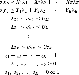
where L and U are the lower bound and upper bound, which are usually of the values 0 and ∞, respectively. The e is a very nonarchimedean small number that in practice is generally taken to be 10-6. Finally, the z 1, z 2, … , and z K are binary 0–1 numbers, which allow for evaluating DMUo with respect to the DMUs of one group at a time. Let E o,k be the efficiency of DMUo measured with respect to the DMUs of group k, where k ranges from 1 to K. Thus, K optimizations are needed in the evaluation of DMUo. The optimal efficiency of DMUo, E o, is decided as the minimum of {E o,1, E o,2, … . , E o,K}. The efficiencies of the remaining (n − 1) DMUs can be obtained in a similar manner.
2.2. Bilateral comparisons approach
The main idea of bilateral comparisons is that each DMU is only evaluated based on intergroup comparison rather than both inter- and within-group comparisons by CEBDS. That is, for each pair of groups, each DMU of one group is evaluated with respect to the DMUs of the opposite group and vice versa. Therefore, for a total of K groups, there will be K!/(2! × (K − 2)!) bilateral comparisons. Let DMUa be an arbitrary DMU of group 1 to be evaluated, and E a,2 denotes the efficiency of DMUa with respect to the DMUs of group 2. Then E a,2 is obtained by solving the following model:
E a,2 = min θ
subject to
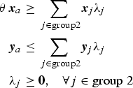
where xa and ya are the input and output vectors for DMUa. The efficiency of each DMU of group 2 with respect to DMUs in group 1 can be easily obtained in a similar manner.
3. PROPOSED PROCEDURE
Assume that there are n experiments in Taguchi's OA of f factors with r responses. The proposed procedure for solving the multiresponse problem in Taguchi method is outlined in the following steps:
Step 1. Consider experiment j (j = 1, … , n) as DMUj. Typically, the relative efficiency of DMUj, which is calculated as the ratio of the sum of the weighted outputs relative to the sum of the weighted inputs, is enhanced when the sum of the weighted outputs is increased and/or the sum of the weighted inputs is decreased. Consequently, the inputs and outputs of DMUj are selected based on the following:
a. If all responses are STB type, which is preferred at minimum, then set all responses as the inputs and set a unit (one) as the output. Conversely, if all the responses are LTB type, which is preferred at maximum, then set all responses as the outputs and set a unit (one) as the input.
b. If all responses are NTB type, then calculate the quality loss L for each response based on the form (Tong et al., Reference Tong, Su and Wang1997)
(4)where ȳ and s are the average and standard deviation of response y, respectively, while c is the quality loss coefficient. Set the L(y) values, which are preferred at minimum, as the inputs and set one as the output.
c. If the responses are a mix of the three response types, set the STB type response and the L(y) values of the NTB type response as inputs, while the LTB type response as the output.
Step 2. Assume factor l of K levels is among the f process factors of OA. Divide the n DMUs into K groups each at the same factor level. Similarly, divide the n DMUs into groups for all of the other (f − 1) process factors. Select the DEA approach for measuring the efficiency of DMUj. If CEBDS approach is selected, perform steps 3 and 4; if bilateral comparisons approach is chosen, conduct steps 5 and 6. Then, go to step 7.
Step 3. For each of the f factors, evaluate the efficiency of DMUj (j = 1, … , n) by solving the CEBDS model. That is, for factor l the E j,k of DMUj is evaluated by solving the CEBDS model with the inputs and outputs of group k (k = 1, … , K). Thus, K optimizations are needed to measure DMUj. Then, identify the optimal efficiency of DMUj, E j, as the minimum of {E j,1, … , E j,K} for all j values.
Step 4. Determine the optimal factor levels for multiresponses using the efficiencies measured by the CEBDS approach. That is, calculate the efficiency of each factor level as the average of E j values for the DMUjs at that level. Then, identify the factor level that maximizes the level efficiency as the optimal level of that factor.
Step 5. For each of the f factors, measure the efficiency E j of each DMUj by solving the bilateral comparisons model. That is, K!/(2! × (K − 2)!) bilateral comparisons are performed for factor l. For each bilateral comparison between a pair of groups, a DMU of one group is evaluated with respect to the DMUs of the opposite group and vice versa.
Step 6. Decide the optimal factor levels for multiresponses using the efficiencies obtained by bilateral comparisons approach. That is, estimate the level efficiency as the average of the E j,k values at that factor level. Identify the factor level that minimizes the level efficiency as the optimal level of that factor.
Step 7. Estimate the anticipated improvement in each response, because of setting all f factors at optimal levels. Compare the anticipated improvement by adopting the proposed procedure with those obtained from other approaches.

4. ILLUSTRATIONS
Three case studies, which were investigated by other approaches that appeared in the literature, are employed to illustrate the proposed procedure.
4.1. Optimization of polysilicon deposition process
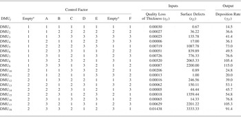
This case study is considered by Phadke (Reference Phadke1989), which aimed at improving the quality of polysilicon process. The three desired responses (r = 3) were thickness (the NTB type response, target is 3600 Å), surface defects (the STB type response), and deposition rate (the LTB type response). Six process factors (f = 6), each at three levels, were chosen, including deposition temperature (A), deposition pressure (B), nitrogen flow (C), silane flow (D), settling time (E), and cleaning method (F). The initial condition was A2B2C1D3E1F1. The L18 OA shown in Table 1 was selected to investigate these factors simultaneously.
Experimental data of the polysilicon process

aEmpty columns are used to estimate the error term.
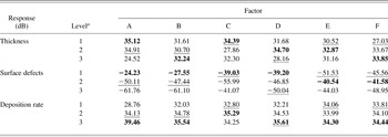
The Taguchi method was employed to optimize each of the three responses separately. The calculated average S/N ratio for each factor level is shown in Table 2, where the combination of optimal factor levels for thickness, surface defects, and deposition rate are A1B3C1D2E2F3, A1B1C1D1E2F2, and A3B3C2D3E3F3, respectively. Obviously, there is a conflict about the optimal factor levels for all responses. The combination of optimal factor levels was then decided by engineering judgment as A1B2C1D3E2F2.
The average S/N ratio of each factor level for the polysilicon process

aInitial and optimal factor levels are identified by underscored and bold type, respectively.
The proposed procedure is implemented for solving the three responses problem in the Taguchi method for the polysilicon process as follows:
Step 1. In the L18 array, 18 experiments (n = 18) were conducted as shown in Table 1, where each experiment is considered as a DMU. The inputs and outputs of each DMU are decided as follows. The quality loss of thickness, which is calculated by Eq. (4), and surface defects are set as the inputs, whereas the deposition rate is set as the output for all the 18 DMUs.
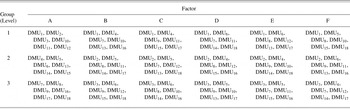
Step 2. Six process factors (A to F) are investigated in this case study. For each factor, the 18 DMUs are then divided into groups, each at the same factor level, as shown in Table 3. For illustration, factor A is assigned at three levels; A1, A2, and A3. As a result, the 18 DMUs are divided into three groups each of 6 DMUs. That is, group 1 contains DMU1 to DMU3 and DMU10 to DMU12 at A1, group 2 includes DMU4 to DMU6 and DMU13 to DMU15 at A2, and group 3 consists of DMU7 to DMU9 and DMU16 to DMU18 at A3. Similarly, the 18 DMUs are divided into groups for factors B to E.
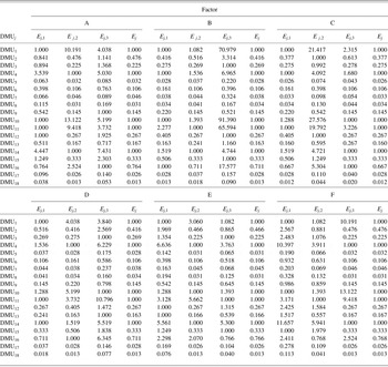
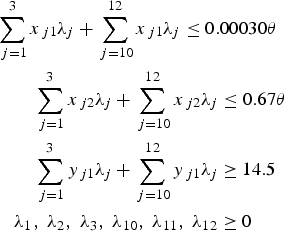
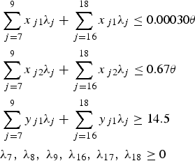
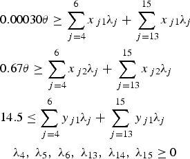
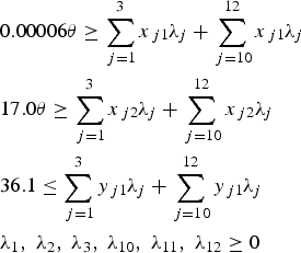
Step 3. For each of the factors A to F, the efficiencies of the 18 DMUs are separately measured by solving the CEBDS model. Table 4 summarizes the obtained DMU's efficiencies for all factors. Let x j1 and x j2 be the two inputs, and y j1 is the output of DMUj. For factor A in Table 4, DMU1 is evaluated as follows. The efficiency, E 1,1 of DMU1 with respect to the 6 DMUs of group 1 is obtained by setting z 1 = 1, z 2 = z 3 = 0 and solving the following model:
E 1,1 = min θ
subject to
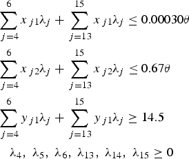
The E 1,1 is measured as 1.000.Similarly, the efficiency of DMU1 with respect to the six DMUs of group 2, E 1,2, is obtained by setting z 2 = 1 and z 1 = z 3 = 0 and solving the following model:
E 1,2 = min θ
subject to
The E 1,2 is evaluated as 10.191.Finally, the efficiency of DMU1 with respect to the six DMUs of group 3, E 1,3, is obtained by setting z 3 = 1 and z 1 = z 2 = 0 and solving the following model:
E 1,3 = min θ
subject to
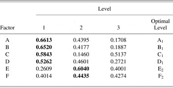
The E 1,3 is evaluated 4.038. The optimal efficiency of DMU1, E 1, is then decided as 1.000; which is the minimum of {E 1,1, E 1,2, E 1,3}. The E 2 to E 18 for DMU2 to DMU18 are evaluated in a similar manner. The E j values for the 18 DMUs using the CEBDS approach for each of the factors B to F are obtained similarly.Step 4. The level efficiency is calculated as the average of the E j values measured using the CEBDS approach for the DMUs at that factor level. Table 5 displays the calculated efficiency of all factor levels. For illustration, the efficiency of A1, 0.6613, is calculated as the sum of the efficiencies for the six DMUs at level 1 divided by six. Similarly, the efficiencies for A2 and A3 are calculated as 0.4395 and 0.1708, respectively. Obviously, the largest level efficiency for factor A corresponds to A1, and hence, the optimal level of factor A is selected at A1. In a similar manner, the optimal levels for factors B to F are decided at B1, C1, D1, E2, and F2, respectively.
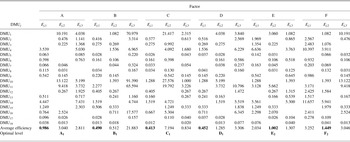
Step 5. For each of the factors A to F, the efficiencies for the 18 DMUs are individually calculated by solving the bilateral comparisons model. Table 6 displays the obtained efficiencies for all factors. For illustration, in Table 6 three bilateral comparisons (=3!/(2! × (3 − 2)!) are conducted for factor A: between groups 1 and 2, groups 1 and 3, and groups 2 and 3. For instance, in the bilateral comparisons between groups 1 and 2, the efficiencies of DMU1, DMU2, DMU3, DMU10, DMU11, and DMU12 of group 1 are measured with respect to DMU4, DMU5, DMU6, DMU13, DMU14, and DMU15 of group 2, and vice versa. That is, the efficiency of DMU1 with respect to the 6 DMUs of group 2, E 1,2, is obtained by solving the following model:
E 1,2 = min θ
subject to
The E 1,2 is measured as 10.191. The E 2,2, E 3,2, E 10,2, E 11,2, E 12,2 are evaluated by solving the bilateral comparison model in a similar way. Each of DMU4, DMU5, DMU6, DMU13, DMU14, and DMU15 of group 2 is then evaluated with respect to the six DMUs of group 1. For instance, the efficiency of DMU4 with respect to the six DMUs of group 1, E 4,1, is measured by solving the following:E 4,1 = min θ
subject to
The E 4,1 is calculated as 3.539. In a similar manner, the E 5,1, E 6,1, E 13,1, E 14,1, E 15,1 are evaluated. The other two bilateral comparisons for factor A are conducted similarly. This step is repeated to obtain the efficiencies for 18 DMUs by the bilateral comparisons approach for factors B to F. It is obvious that the efficiencies measured by the bilateral comparisons approach in Table 6 are the same as those obtained by the CEBDS approach in Table 4. The reason is that the DMU's efficiency is evaluated by an intergroup comparison of both approaches in a similar way.
Step 6. The level efficiency is calculated as the average of the E j,k values evaluated by the bilateral comparisons approach at that factor level. Table 6 lists the level efficiency for all factor levels. For illustration, the efficiency of A1, 0.986, is calculated as the average of E j,1 values. Similarly, the efficiency for A2 and A3 are calculated as 3.040 and 2.811, respectively. The minimum of {0.986, 3.040, 2.811} corresponds to A1, and hence, the optimal level of factor A is decided at A1. In a similar manner, the optimal levels for factors B to F are decided at B1, C1, D1, E2, and F2, respectively. In this case study, the proposed procedure provides the same optimal factor levels for both DEA approaches. However, the bilateral comparisons approach results in a sharper discrimination among various factor levels, as noted from the differences between the level efficiencies for each factor, and requires less computational effort because of conducting only intergroup comparison than the CEBDS approach, which performs both the inter- and within-group comparisons.
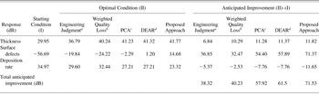
Step 7. The anticipated improvements in thickness, surface defects, and deposition rate because of setting the six factors at optimal levels (A1B1C1D1E2F2) are calculated using the S/N ratio averages listed in Table 2. The obtained anticipated improvements in the three responses by following the proposed procedure are summarized in Table 7. This case study was investigated by engineering judgment (Phadke, Reference Phadke1989), the sum of the weighted normalized quality losses (Tong et al., Reference Tong, Su and Wang1997), PCA (Su & Tong, Reference Su and Tong1997), and DEAR (Liao & Chen, Reference Liao and Chen2002). The anticipated improvements obtained from these approaches are also displayed and compared in Table 7.
In Table 7, the overall average of the 18 S/N ratio averages for thickness is calculated 31.52 dB. The sum of differences between the S/N ratio averages at the optimal level and the overall average is calculated 10.25 dB. Then, the optimal condition for thickness equals 41.77 dB. The anticipated improvement in thickness of 11.82 dB (= 41.77 – 29.95) is the largest among all approaches. The optimal conditions and anticipated improvements for surface defects and deposition rate are estimated similarly. It is noted that surface defects are significantly reduced by 71.37 dB, which is also the largest among all approaches. However, the anticipated improvement in deposition rate is −11.65 dB, which is the worst of all approaches. Despite that, the proposed procedure provides the largest total anticipated improvement, and thus should be considered the most effective procedure for solving the multiresponse problems in the Taguchi method among all used approaches for the polysilicon process.
The DMU groups of each factor for the polysilicon process

The efficiency for all DMUs using the CEBDS approach for all process factors

The level of efficiency for the polysilicon process using the CEBDS approach

The optimal levels are in bold.
The efficiency of all DMUs for the polysilicon process using the bilateral comparisons approach

Comparisons of the anticipated improvements for the polysilicon process

aPhadke (Reference Phadke1989).
bTong et al. (Reference Tong, Su and Wang1997).
cSu and Tong (Reference Su and Tong1997).
dLiao and Chen (Reference Liao and Chen2002).
4.2. Optimization of gear hobbing operation
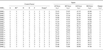
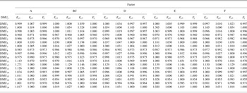
Jeyapaul et al. (Reference Jeyapaul, Shahabudeen and Krishnaiah2006) investigated the effect of machining parameters on multiple performance characteristics (profile and helix variation) pertaining to a gear-hobbing operation using the GA. Four responses were studied, including left profile (LP) error, right profile (RP) error, left helix (LH) error, and right helix (RH) error, which all are considered as the STB type responses. Six controllable factors were selected, including direction of hobbing (A, at two levels), number of passes (B, at two levels), source of hob (C, at two levels), feed (D, at three levels), speed (E, at three levels), and job run out (F, at three levels). The initial factor levels were decided as A1B2C2D2E1F3. The L18 OA was selected for providing the experiment design. However, the L18 array can accommodate one factor at two levels and seven factors each at three levels. Therefore, the two factors B and C were combined into one factor (BC) of B1C1 at level 1, B2C1 at level 2, and B2C2 at level 3. The proposed procedure for solving the problem of profile and helix errors is implemented as follows:
Step 1. As shown in Table 8, the L18 array results in 18 DMUs to be evaluated. For each DMU, all of the LP, RP, LH, and RH errors are set as the inputs, whereas a unit (one) is set as the output.
Step 2. For each of the factors A to F, the 18 DMUs at the same factor level are set into one group. From Table 8, two groups are formed for factor A: DMU1 to DMU9 at A1 are set in group 1, whereas DMU10 to DMU18 at A2 are set in group 2. However, the 18 DMUs are divided into three groups for each of the factors BC, D, E, and F.
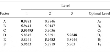
Step 3. For each of the factors A to F, the efficiencies for the 18 DMUs are individually measured by solving the CEBDS model and listed in Table 9. For factor A in Table 9, the calculated E 1,1 and E 1,2 of DMU1 are 0.999 and 1.007, respectively. Hence, E 1 equals 0.999, the minimum of {0.999, 1.007}. The values of E 2 to E 18 are evaluated in a similar manner. For each of the factors BC, D, E, the efficiencies for the 18 DMUs can be independently evaluated by solving the CEBDS model similarly.
Step 4. The level efficiency is calculated as the average of the E j values obtained by the CEBDS approach for the DMUs at that factor level in Table 10 for all factor levels. In Table 10, the level efficiencies for factors B and C are obtained from the combined factor BC as follows. As mentioned earlier, B1C1, B2C1, and B2C2 are assigned at levels 1, 2, and 3 of factor BC, respectively. Thus, the efficiency of B1 (=5.9441) equals the efficiency of level 1 for BC, while the efficiency of B2 (=5.9147) is estimated as the average efficiency for levels 2 and 3. Conversely, the efficiency of C1 (=5.93495) is calculated as the average efficiency for levels 1 and 2 of BC, whereas the efficiency of C2 (=5.9036) is equal to the efficiency of level 3. Moreover, the combination of optimal factor levels for factors A to F in this table is decided as A1B1C1D3E2F1.
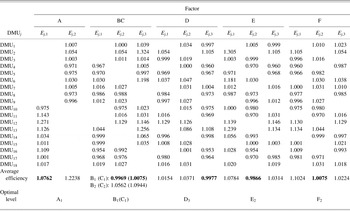
Step 5. For each of the factors A to F, the efficiencies for the 18 DMUs are independently evaluated by solving the bilateral comparisons model. In this case study, the efficiencies for the 18 DMUs are measured by conducting one bilateral comparisons for factor A; each of DMU1 to DMU9 at A1 is evaluated with respect to all of DMU10 to DMU18 at A2 and vice versa. However, the efficiencies for the 18 DMUs are calculated by performing two bilateral comparisons for each of the factors BC to F. Table 11 displays the measured efficiencies for the 18 DMUs by the bilateral comparisons approach.
Step 6. The level efficiency is calculated as the average of the E j values measured by the bilateral comparisons approach for that factor level and also displayed in Table 11. In this table, the combination of optimal factor levels is determined as A1B1C1D3E2F2.
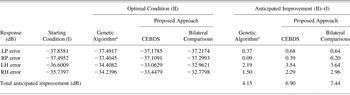
Step 7. The anticipated improvements in LP, RP, LH, and RH errors, because of setting process factors at the combinations of optimal factor levels, are displayed in Table 12 and compared with the anticipated improvements by GA (Jeyapaul et al., Reference Jeyapaul, Shahabudeen and Krishnaiah2006). Obviously, the anticipated improvements in Table 12 using the proposed procedure are larger than those by the GA for all four responses. This shows that the proposed procedure outperforms the GA in solving the multiresponse problem for the gear-hopping operation. Moreover, it can easily be observed that using the bilateral comparisons approach to measure DMU's efficiency in the proposed procedure results in better total anticipated improvements than the CEBDS approach.
Experimental data of the gear hobbing operation

aCombined factor.
bEmpty columns are used to estimate the error term.
The efficiency of DMUs for the gear hobbing operation using the CEBDS approach

The level efficiency for the gear hobbing operation using the CEBDS approach

The efficiency of DMUs for the gear hobbing operation using the bilateral comparisons approach

Comparisons of anticipated improvements for the gear hobbing operation

aJeyapaul et al. (Reference Jeyapaul, Shahabudeen and Krishnaiah2006).
4.3. Optimization of hard disk drive
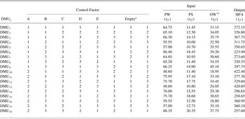
This case study was conducted by the Industrial Technology Research Institute in Taiwan, to improve the quality of the hard disk drive. Four responses were chosen, including 50% pulse width (PW, the STB type response), peak shift (PS, the STB type response), over write (OW, the LTB type response), and high-frequency amplitude (HFA, the LTB type response). Five controllable factors were investigated involving disk writability (A, two levels), magnetization width (B, three levels), gap length (C, three levels), coercivity of media (D, three levels), and rotational speed (E, three levels). The initial factor levels were A1B1C2D2E3. The L18 OA was utilized for conducting the 18 experiments as shown in Table 13.
Experimental data of a hard disk drive

aEmpty columns are used to estimate error terms.
bOW′ = −1 × OW.
Phadke (Reference Phadke1989) mentioned that the STB, NTB, and LTB type responses should have nonnegative values. However, in this case study the original OW values are negative, with the desired target being (close to) zero. Because maximizing a quality response is equivalent to minimizing the negative of that response, the OW is multiplied by −1 and treated as the STB type response. Let OW′ = −1 × OW. Then, the proposed procedure for solving the multiresponse problem for this case study is briefly outlined as follows:
Step 1. In this case study, 18 DMUs are considered. All of the PW, PS, and OW′ are set as the inputs, whereas the HFA is set as the output.
Step 2. For each of the factors A to E, the 18 DMUs are divided into groups, each at the same factor level. That is, the 18 DMUs are divided into two groups for factor A, whereas they are divided into three groups for factors B to E.
Step 3. For each of the factors A to E, the efficiencies for the 18 DMUs are separately measured by solving the CEBDS model.
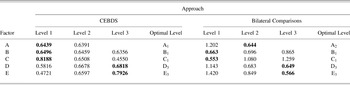
Step 4. The level efficiency is obtained for all factor levels and displayed in Table 14. Using the CEBDS approach, it is noted in Table 14 that the combination of optimal factor levels is determined as A1B1C1D3E3.
Step 5. For each of the factors A to E, the efficiencies for the 18 DMUs are individually evaluated by solving the bilateral comparisons model.
Step 6. The level efficiency is calculated for all factor levels and also tabulated in Table 14. Using the bilateral comparisons approach, the combination of optimal factor levels in this table is decided as A2B1C1D3E3.
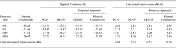
Step 7. The anticipated improvements in PW, PS, OW′, and HFA because of setting process factor levels at A1B1C1D3E3 and A2B1C1D3E3 are displayed and compared with the anticipated improvements by PCA (Su & Tong, Reference Su and Tong1997) and DEAR (Liao & Chen, Reference Liao and Chen2002) in Table 15. It is clear that the proposed procedure, using either the CEBDS or the bilateral comparisons approach, provides the largest total anticipated improvements and thus outperforms both PCA and DEAR. However, the bilateral comparisons approach is superior to CEBDS approach in the proposed procedure for solving the multiresponse problem in the Taguchi method for the hard disk drive.
The level efficiency for a hard disk drive using both DEA approaches

Comparisons of anticipated improvements for a hard disk drive

aSu and Tong (Reference Su and Tong1997).
bLiao and Chen (Reference Liao and Chen2002).
cThe OW was multiplied by 1 and then treated as an STB response; thus, the initial condition is considered to be −31.51.
5. RESEARCH RESULTS
Today's highly competitive markets urge process/product engineers to seek an efficient approach for solving the multiresponse problem in the Taguchi method. Therefore, this problem has received considerable research attention. In the previous section, the proposed procedure is implemented for solving the multiresponse problem in the Taguchi method for the polysilicon process, gear-hobbing operation, and the hard disk drive. The computational results showed several advantages of the proposed procedure including the following:
1. Effectiveness in improving performance: It is obvious in Tables 7, 12, and 15 that the proposed procedure provides the largest anticipated improvement among all previously used approaches for solving the multiresponse problem. This shows the effectiveness of the proposed procedure in deciding the combination of factor levels that enhances process/product performance.
2. No a priori knowledge of response weights needed: Compared with engineering judgment (Phadke, Reference Phadke1989), the sum of weighted S/N ratios (Tai et al., Reference Tai, Chen and Wu1992) and the sum of the weighted normalized quality losses (Tong et al., Reference Tong, Su and Wang1997), the proposed procedure does not require a priori knowledge of response weights, and thus it reduces the uncertainty in the decision-making process.
3. Less complex and thus easily understood and applied by process/product engineers: Compared with regression techniques (Pignatello, Reference Pignatello1993; Reddy et al., Reference Reddy, Nishina and Subash Babu1997) and the GA (Jeyapaul, 2006), the proposed procedure is less complex and requires minimal statistical skills. This make it easily understood and widely applied by process/product engineers.
4. No rigid assumptions and trade-off: Compared with PCA (Su & Tong, Reference Su and Tong1997; Antony, Reference Antony2000), the proposed procedure is not based on rigid assumptions and it eliminates the need for trade-off in selecting the optimal factor levels when more than one principal component is greater than 1 in PCA.
5. Sharper discrimination among efficient DMUs and thus provides more reliable efficiency scores: Compared with DEAR (Liao & Chen, Reference Liao and Chen2002), the CEBDS and the bilateral comparisons approaches are very effective in measuring and providing sharper discriminations among the efficiencies for a set of DMUs, and thus provide more reliable efficiency scores than the CCR model adopted in the DEAR approach. Consequently, the proposed approach outperforms the DEAR approach in solving the multiresponse problem for the polysilicon process and the hard disk drive.
These advantages will attract process/product engineers to apply the proposed procedure for solving the multiresponse problem in parameter design for a wide range of manufacturing applications on the Taguchi method. At the organizational level, this procedure can be utilized in comparisons between different systems of multiinputs and/or multioutputs.
6. CONCLUSIONS
This research utilizes DEA approaches for solving the multiresponse problem in the Taguchi method. The CEBDS and the bilateral comparisons approaches in DEA are adopted in the procedure proposed in this research. In this procedure, each experiment in OA is treated as a DMU, with the multiresponses as the inputs and outputs for all DMUs. Then, the efficiency of each factor level, which is calculated as the average of the efficiencies from CEBDS and the bilateral comparisons approaches for that factor, is then used to decide optimal factor levels. Three case studies in manufacturing are provided for illustration, where in all case studies the proposed procedure outperforms the previously used approaches, such as PCA, DEAR, and GA, for solving the multiresponse problems. Moreover, between the two DEA approaches, the bilateral comparisons approach is superior to the CEBDS approach, because the former not only provides sharper discrimination among factor levels and thus provides larger anticipated improvements in the responses, but also requires less computational effort. In conclusion, the proposed procedure can serve as a useful approach for solving the multiresponse problem in the manufacturing applications on the Taguchi method. In addition, DEA is effective for evaluating the performance of DMUs at the organizational level, as well as in manufacturing at the operational level.
ACKNOWLEDGMENT
This research was supported in part by the National Science Council of the Republic of China under Grant NSC96-2221-E-035-039.
Abbas Al-Refaie received his PhD degree in industrial engineering and systems management from Feng Chia University, Taiwan. Dr. Al-Refaie's research interests include statistical quality control, experimental design, and optimization.
Tai-Hsi Wu is a Professor in the Business Administration Department at the National Taipei University, Taiwan. He received his PhD degree from Texas A&M University in 1994. Dr. Wu has published academic papers in a wide variety of journals such as European Journal of Operational Research, Computers and Operations Research, International Journal of Production Research, and Expert Systems With Applications. His research interests include production and operations research, data envelopment analysis, and solving combinatorial optimization problems using heuristic algorithms.
Ming-Hsien Caleb Li is a Professor in the Department of Industrial Engineering and Systems Management at Feng Chia University, Taiwan. His interests are quality engineering, the Taguchi method, experimental design, and statistical quality control.