1 Introduction
The transition of fluid motion from a laminar state to a turbulent state has been an unresolved conundrum in wall-bounded shear flows. Typically, there are three transition regimes for boundary-layer flow, which demonstrate different features during the transition process, namely the K-regime, N-regime and O-regime. The three transition processes are mainly investigated from a spectral point of view and a structure-based view (Rist & Fasel Reference Rist and Fasel1995; Berlin, Wiegel & Henningson Reference Berlin, Wiegel and Henningson1999). The former view usually employs frequency–wavenumber Fourier analysis to obtain the amplification rates of different modes. While a structure-based view mainly examines the spatial/temporal flow structures extracted from experimental or numerical data sets. Generally, when described in terms of frequency–wavenumber ( $\unicode[STIX]{x1D714},\unicode[STIX]{x1D6FD}$), where the
 $\unicode[STIX]{x1D714}$ is the fundamental frequency, and
 $\unicode[STIX]{x1D6FD}$ is the spanwise wavenumber, a K-regime transition is usually initiated by a primary Tollmien–Schlichting wave (T–S wave) (
 $\unicode[STIX]{x1D714},0$) and a pair of symmetric oblique waves (
 $\unicode[STIX]{x1D714},\pm \unicode[STIX]{x1D6FD}$) with the same frequency as that of the primary two-dimensional (2-D) wave. The K-regime is named after Klebanoff, Tidstrom & Sargent (Reference Klebanoff, Tidstrom and Sargent1962), who studied the three-dimensional nature of boundary-layer instability under controlled conditions, and the typical pattern for this regime was characterized as peak and valley regions with very high amplitudes of the perturbations in the peak positions. They determined that a 2-D T–S wave will interact with the mean flow, and then rapidly develop into a three-dimensional (3-D) wave, forming aligned 𝛬-structures, which finally breaks down to turbulence.
For the N-regime transition, an initially primary planar wave ( $\unicode[STIX]{x1D714},0$) interacts with a pair of subharmonic oblique waves with streamwise frequency equal to half the primary wave, i.e. (
 $\unicode[STIX]{x1D714}/2,\pm \unicode[STIX]{x1D6FD}$), to form 𝛬-structures positioned in a staggered order. The N-regime is also called the ‘subharmonic regime’ (Zelman & Maslennikova Reference Zelman and Maslennikova1993) or the ‘H-regime’ after Herbert (Reference Herbert1984), both of who provided theoretical formulations of the resonant amplification of the subharmonic modes. The detailed experimental work on N-regime breakdown was carried out at Novosibirsk (Kachanov, Kozlov & Levchenko Reference Kachanov, Kozlov and Levchenko1977; Kachanov & Levchenko Reference Kachanov and Levchenko1984), where it was determined that the N-regime is also characterized by amplification of a wide low-frequency disturbance around the subharmonic frequency
 $\unicode[STIX]{x1D714}/2$, and growth of disturbances at frequency of
 $n\unicode[STIX]{x1D714}/2$ (
 $n=3,5,7,\ldots$).
Finally, the O-regime discovered by Goldstein & Choi (Reference Goldstein and Choi1989) and Schmid & Henningson (Reference Schmid and Henningson1992), is induced by a pair of oblique waves with equal, but opposite, angles ( $\unicode[STIX]{x1D714},\pm \unicode[STIX]{x1D6FD}$). These oblique waves will drive a rapidly growing zero-frequency mode (
 $0,\pm 2\unicode[STIX]{x1D6FD}$), which is associated with low-speed streaks and/or streamwise vortices. Mutual and self-interactions of the streamwise vortex/streaks and the oblique waves result in the rapid growth of other harmonic waves, and form a pattern of staggered 𝛬-vortices within the subsequent transition.
The similarity between the regimes mentioned above has been assessed (Berlin et al. Reference Berlin, Wiegel and Henningson1999; Schmid & Henningson Reference Schmid and Henningson2001; Boiko et al. Reference Boiko, Dovgal, Grek and Kozlov2012), especially for the K and N regimes (Laurien & Kleiser Reference Laurien and Kleiser1989; Bake, Fernholz & Kachanov Reference Bake, Fernholz and Kachanov2000). The K and N regimes were incorporated into the framework of a wave-resonance concept by Kachanov (Reference Kachanov1987), and it was shown that the two regimes can be transformed to each other depending on the initial conditions (Kachanov Reference Kachanov1994). Bake et al. (Reference Bake, Fernholz and Kachanov2000) compared the late stage of K- and N-regime transition experimentally, and they observed that these two regimes bear a strong similarity in the local processes of nonlinear disturbance and the features of the developing flow structures. Sayadi, Hamman & Moin (Reference Sayadi, Hamman and Moin2013) evaluated the breakdown of K- and N-regimes to turbulence during late-stage transition using direct numerical simulations (DNS), and determined that the flow statistics and near-wall dynamics are similar, which led them to propose that the late-stage transition, manifested by hairpin packets, as a reduced-order model of a turbulent boundary layer.
The previous structure-based investigations of K, N and O transition regimes were mainly focused on the following structures:
(i) 𝛬- or hairpin-shaped structures during late-stage transition, characterised by aligned or staggered order (Sayadi et al. Reference Sayadi, Hamman and Moin2013, Reference Sayadi, Schmid, Nichols and Moin2014);
(ii) negative peaks in the streamwise velocity time traces termed ‘spikes’, occurring in the peak region, which doubled, tripled, etc. downstream, representing strictly a deterministic and periodic structure (Kovasznay, Komoda & Vasudeva Reference Kovasznay, Komoda and Vasudeva1962; Kachanov & Levchenko Reference Kachanov and Levchenko1984; Rist & Fasel Reference Rist and Fasel1995);
(iii) a structure similar to ring-like vortices, termed coherent structures/soliton (SC-soliton), describing the soliton behaviour of velocity spikes (Kachanov Reference Kachanov, Johansson and Alfredsson1991; Kachanov, Ryzhov & Smith Reference Kachanov, Ryzhov and Smith1993; Meyer et al. Reference Meyer, Rist, Borodulin, Gaponenko, Kachanov, Lian, Lee, Fasel and Saric2000; Borodulin et al. Reference Borodulin, Gaponenko, Kachanov, Meyer, Rist, Lian and Lee2002);
(iv) a localized and intensified warped wave front (Hama & Nutant Reference Hama and Nutant1963; Wortmann Reference Wortmann and Krause1981), accompanied by a kinked high-shear layer (Nishioka, Asai & Iida Reference Nishioka, Asai, Iida and Meyer1981), appearing prior to the development of a 𝛬-vortex;
(v) a three-dimensional wavelike structure, termed a soliton-like coherent structure (SCS), appearing farther upstream prior to development of a 𝛬-vortex (Lee Reference Lee1998; Lee & Wu Reference Lee and Wu2008; Chen Reference Chen2013);
(vi) wave packets that involve a T–S wave (Cohen, Breuer & Haritonidis Reference Cohen, Breuer and Haritonidis1991) or spatio-temporal wave front (Bhaumik & Sengupta Reference Bhaumik and Sengupta2014); and
(vii) streaks that are surrounded by warped wave fronts (Boiko et al. Reference Boiko, Westin, Klingmann, Kozlov and Alfredsson1994), or flanked by streamwise vortices (Berlin et al. Reference Berlin, Wiegel and Henningson1999; Bose & Durbin Reference Bose and Durbin2016).
Different hypotheses have been made regarding the mechanisms responsible for the generation of the velocity spikes and low-speed streaks. Some of these hypotheses are correlated with vortical structures (e.g. hairpin vortices), but others are based on non-vortical structures (e.g. wave packets), and there is no current consensus on the relationship between the wave packets and vortices. The similarity between different transition regimes in previous studies usually focused on the late stage of transition, where hairpin vortices (hairpin packets, ring-like vortices or multiple spikes) have already appeared. In the present study, we focus on the coherent wave states (iv)–(v), which emerge during the early nonlinear stages, prior to the appearance of any apparent vortices.
In the classical work of Hama and his colleagues, which employed hydrogen bubble visualization to observe structures within a transitional boundary layer (Hama, Long & Hegarty Reference Hama, Long and Hegarty1957; Hama & Nutant Reference Hama and Nutant1963), they observed that the T–S wave warps three-dimensionally during amplification, acquiring a longitudinal vorticity component along its swept-back front. This region of concentrated high-shear layer, which appears as an inflection in vertical hydrogen bubble timelines (a ‘kink’), subsequently develops into a hairpin-shaped, discrete vortex. This localized and intensified warped or kinked structure was considered as the source of subsequent hairpin-shaped vortices. Here, we refer to this kinked structure as a ‘warped wave front’ (WWF). This warping process and kinked profiles were frequently observed experimentally or numerically in transitional boundary layers (Wortmann Reference Wortmann and Krause1981; Laurien & Kleiser Reference Laurien and Kleiser1989; Boiko et al. Reference Boiko, Westin, Klingmann, Kozlov and Alfredsson1994; Rist & Fasel Reference Rist and Fasel1995; Lee Reference Lee1998; Zhao, Yang & Chen Reference Zhao, Yang and Chen2016). However, the roles of a WWF in transition are often underrated, and the manner in which a WWF originates and evolves is not well understand. This emphasizes the need to examine the details of the warping process and the development of a WWF prior to the emergence of 𝛬-vortices. A hypothesis based on a three-dimensional wave-like structure, has been proposed as an explanation of the velocity profile ‘kink’ (Lee Reference Lee1998, Reference Lee2000). Such a 3-D wavelike structure was observed within the whole boundary layer, covering the near-wall region to the outer edge, in almost all dynamic processes for both the early and later stages of a transitional boundary layer. The structure was later termed a soliton-like coherent structure (Lee & Chen Reference Lee, Chen, Ged-el Hak and Tsai2006; Lee & Li Reference Lee and Li2007; Lee & Wu Reference Lee and Wu2008). Using DNS, Chen (Reference Chen2013) confirmed the existence of a SCS and its dominant role in the vortex evolution process. However, the above mentioned experimental results were based on flow visualizations or hot-wire measurements, while the numerical study is mainly based on the assessment of iso-surfaces or instantaneous fields.
The objective of the present paper is to characterise the 3-D wave structures during the early nonlinear stage of transition, and to understand how a WWF evolves into a 𝛬-vortex. In a Lagrangian framework, we focus on a piece of history of the flow, employing a visualization method based on tracking the basic trajectories of marked particles (Jiang Reference Jiang2019a,Reference Jiangb). We use both time-resolved tomographic particle image velocimetry (tomo-PIV) measurements and the solution of nonlinear parabolized stability equations (NPSE) to obtain three-dimensional data sets of the spatial–temporal transition process. These data sets are then used to examine the details of the wave-warping process, and to examine the relationship between 3-D waves, low-speed streaks, and 𝛬-vortices in transitional boundary layers. The remainder of this paper is organized as follows: in § 2, the method of NPSE is described, including the numerical settings for the three transition regimes and the method of Lagrangian tracking; in § 3, the results of the NPSE calculations (including K-regime, O-regime and N-regime) are presented; in § 4, the experimental procedure is described and the results of the experiments (only the K-regime) are compared with the simulations; in § 5, the underlying physical mechanism is discussed, and a possible unified transition path is proposed based on the experimental/numerical comparisons; and conclusions are given in § 6.
2 Method of numerical simulation
2.1 Nonlinear parabolized stability equation
The NPSE are suitable for investigating both linear and weakly nonlinear evolutions of disturbances. The detailed formulation of the NPSE can be found in Bertolotti, Herbert & Spalart (Reference Bertolotti, Herbert and Spalart1992) and Chang & Malik (Reference Chang and Malik1994). Thus, only a brief introduction is given here. In the NPSE formulation, the disturbance is decomposed into a rapidly varying wave-like part and a slowly varying shape function as follows:
 $$\begin{eqnarray}\unicode[STIX]{x1D6F9}(x,y,\unicode[STIX]{x1D6FD}_{z},t)=\bar{\unicode[STIX]{x1D6F9}}(x,y)+\mathop{\sum }_{m,n}\hat{\unicode[STIX]{x1D6F9}}_{mn}(x,y)\exp \left(\text{i}\int _{0}^{x}\unicode[STIX]{x1D6FC}_{mn}\,\text{d}x-\text{i}\unicode[STIX]{x1D714}_{m}t+\text{i}n\unicode[STIX]{x1D6FD}_{z}\right),\end{eqnarray}$$
where  $\unicode[STIX]{x1D6F9}\equiv (u,v,w,p)$;
 $\bar{\unicode[STIX]{x1D6F9}}$ denotes the basic state;
 $\hat{\unicode[STIX]{x1D6F9}}_{mn}\equiv (\hat{u} ,\hat{v},{\hat{w}},\hat{p})_{mn}$ are the shape functions for the Fourier mode (
 $m,n$);
 $\unicode[STIX]{x1D6FD}_{z}$ denotes the spanwise wave number; and
 $\unicode[STIX]{x1D6FC}_{mn}$ and
 $\unicode[STIX]{x1D714}_{m}$ are the associated streamwise (complex) wavenumber and frequency. The negative imaginary part of
 $\unicode[STIX]{x1D6FC}_{mn}$,
 $-\unicode[STIX]{x1D6FC}_{i}$, represents the growth rate of the mode, while the real part is related to the phase velocity as
 $$\begin{eqnarray}c_{mn}\equiv \frac{\unicode[STIX]{x1D714}_{m}}{\text{Re}(\unicode[STIX]{x1D6FC}_{mn})},\end{eqnarray}$$
where  $\text{Re}$ denotes the real part. All the variables are non-dimensionalized using the free-stream velocity
 $U_{\infty }$ and the fixed characteristic thickness
 $\unicode[STIX]{x1D6FF}_{0}=\unicode[STIX]{x1D6FF}(x_{0})=(\unicode[STIX]{x1D708}\tilde{x}_{0}/U_{\infty })^{1/2}$, where
 $\tilde{x}_{0}$ is the initiation location where disturbances are forced, and
 $\unicode[STIX]{x1D708}$ is the kinematic viscosity of the fluid. Note that
 $x_{0}=\tilde{x}_{0}/\unicode[STIX]{x1D6FF}_{0}=U_{\infty }\unicode[STIX]{x1D6FF}_{0}/\unicode[STIX]{x1D708}=R_{0}$ and
 $R=(x/x_{0})^{1/2}R_{0}$, where
 $R_{0}$ and
 $R$ are Reynolds numbers based on
 $\unicode[STIX]{x1D6FF}_{0}$ and
 $\unicode[STIX]{x1D6FF}(x)$, respectively.
The mode shape,  $\hat{\unicode[STIX]{x1D6F9}}_{mn}(x,y)$, is assumed to be a slowly varying function of the streamwise coordinate,
 $x$, so that its second derivative with respect to
 $x$ is negligible. Substituting (2.1) into the Navier–Stokes equation and subtracting the mean-flow equation yields the governing equations for the shape functions of each mode
 $(m,n)$ as
 $$\begin{eqnarray}({\mathcal{L}}_{0}+{\mathcal{L}}_{1})\hat{\unicode[STIX]{x1D6F9}}_{mn}+{\mathcal{L}}_{2}\frac{\unicode[STIX]{x2202}\hat{\unicode[STIX]{x1D6F9}}_{mn}}{\unicode[STIX]{x2202}x}+\frac{\text{d}\unicode[STIX]{x1D6FC}_{mn}}{\text{d}x}{\mathcal{L}}_{3}\hat{\unicode[STIX]{x1D6F9}}_{mn}={\mathcal{F}}_{mn},\end{eqnarray}$$
where  ${\mathcal{L}}_{0}$ contains the linear–parallel terms,
 ${\mathcal{L}}_{1}$ contains the non-parallel mean-flow terms,
 ${\mathcal{L}}_{2}$ and
 ${\mathcal{L}}_{3}$ arise from the non-parallel disturbance terms and
 ${\mathcal{F}}_{mn}$ is the nonlinear forcing term. For expression of the operators
 ${\mathcal{L}}_{0}$,
 ${\mathcal{L}}_{1}$,
 ${\mathcal{L}}_{2}$,
 ${\mathcal{L}}_{3}$ and
 ${\mathcal{F}}_{mn}$ refer to Guo & Tang (Reference Guo and Tang2010) and Zhu et al. (Reference Zhu, Lee, Chen, Wu, Chen and Gad-el Hak2018).
This system of equations is parabolic and thus requires boundary and initial conditions. The initial conditions are provided by the results from the linear stability theory (Chen, Zhu & Lee Reference Chen, Zhu and Lee2017). The boundary conditions are
 $$\begin{eqnarray}\displaystyle \hat{u} _{mn},\hat{v}_{mn},{\hat{w}}_{mn}=0,\quad \text{at}~y=0~\text{and}~\infty , & & \displaystyle\end{eqnarray}$$
which correspond to the no-slip boundary condition at the wall, and vanishing velocity disturbances as  $y\rightarrow \infty$. However, for the mean-flow distortion,
 $\hat{\unicode[STIX]{x1D6F9}}_{00}$, the infinity condition for the wall-normal velocity is replaced by
 $$\begin{eqnarray}\frac{\unicode[STIX]{x2202}\hat{v}_{00}}{\unicode[STIX]{x2202}y}=0,\quad \text{at}~y=\infty ,\end{eqnarray}$$
which accounts for the boundary-layer growth. Provided initial and boundary conditions, equation (2.3) was solved by marching in the streamwise direction using an Euler backward scheme. At each marching step, the mode function as well as other stability characteristics of the mode (including growth rates, phase velocities, etc.) were obtained.
There is still ambiguity in the  $x$-dependence between
 $\hat{\unicode[STIX]{x1D6F9}}_{mn}$ and
 $\unicode[STIX]{x1D6FC}_{mn}$. In this study, the wavenumber at each station was updated as
 $$\begin{eqnarray}\unicode[STIX]{x1D6FC}^{new}=\unicode[STIX]{x1D6FC}^{old}-\text{i}\frac{1}{E}\int _{0}^{\infty }\left(\hat{u} ^{\ast }\frac{\unicode[STIX]{x2202}\hat{u} }{\unicode[STIX]{x2202}x}+\hat{v}^{\ast }\frac{\unicode[STIX]{x2202}\hat{v}}{\unicode[STIX]{x2202}x}+{\hat{w}}^{\ast }\frac{\unicode[STIX]{x2202}{\hat{w}}}{\unicode[STIX]{x2202}x}\right)\text{d}y,\end{eqnarray}$$
where
 $$\begin{eqnarray}E\equiv \int _{0}^{\infty }(|\hat{u} |^{2}+|\hat{v}|^{2}+|{\hat{w}}|^{2})\,\text{d}y,\end{eqnarray}$$
with the asterisk denoting the complex conjugate. This updating process is continued until the largest change is less than  $10^{-5}$.
2.2 Numerical setting and mode description
In the present study, in the language of frequency–wavenumber, the notation ( $\unicode[STIX]{x1D714}$,
 $\unicode[STIX]{x1D6FD}$) is used, where
 $\unicode[STIX]{x1D714}$ and
 $\unicode[STIX]{x1D6FD}$ denote the streamwise frequency and spanwise wavenumber, respectively. For simplicity,
 $\unicode[STIX]{x1D714}$ and
 $\unicode[STIX]{x1D6FD}$ are normalized with the corresponding values of the primary waves. For K-regime transition, a 2-D T–S wave of normalized frequency
 $F=\unicode[STIX]{x1D714}/R_{0}=106\times 10^{-6}$, and a pair of oblique waves at the same frequency, are introduced at the initiation point (
 $R_{0}=400$), i.e. modes (1, 0) and (1,
 $\pm 1$). Therefore, the corresponding non-dimensional period is
 $T=2\unicode[STIX]{x03C0}/(R_{0}F)=148.2$, and the streamwise wavelength
 $\unicode[STIX]{x1D706}_{x}\approx 50$. The spanwise wavenumber
 $\unicode[STIX]{x1D6FD}$ is chosen as 0.05 to make the spanwise wavelength
 $\unicode[STIX]{x1D706}_{z}\sim O(\unicode[STIX]{x1D706}_{x})$, i.e.
 $\unicode[STIX]{x1D706}_{z}\approx 126$. The amplitude
 ${\mathcal{A}}$ for the primary 2-D wave is
 $0.2\,\%\,U_{\infty }$, and
 $0.14\,\%\,U_{\infty }$ for the oblique waves. For N-regime transition, the same 2-D T–S wave as employed for the K-regime transition is forced with a pair of oblique waves at half the frequency, i.e. (1, 0) and (0.5,
 $\pm 1$). For O-regime transition, only a pair of oblique waves are introduced, namely (1,
 $\pm 1$). The detailed information for the initial forcing wave components applied at the initiation location for the K, N and O transition scenarios is shown in table 1.
Numerical settings for all three simulations. A normalized notation ( $\unicode[STIX]{x1D714},\unicode[STIX]{x1D6FD}$) is used in mode description. The first digit indicates multiples of the fundamental streamwise frequency and the second digit refers to multiples of the fundamental spanwise wavenumber.

2.3 Method of Lagrangian tracking
Three-dimensional data sets of the spatial-temporal transition process are obtained from the solution to the NPSE and also from the tomo-PIV measurements. These data sets are used to reconstruct flow structures by employing Lagrangian tracking of marked particles. So, it is helpful to revisit the concepts of the pathlines, streaklines and timelines.
A particle pathline shows the sequence of particle locations over time as a particle moves through a fluid medium. It is determined by integrating an ordinary differential equation over real time
 $$\begin{eqnarray}\boldsymbol{V}(\boldsymbol{X}(t),t)=\text{d}\boldsymbol{X}(t)/\text{d}t.\end{eqnarray}$$
Determining how a vector field changes with time from pathlines is possible, if the vector field is not too complicated. However, the information provided by a pathline is limited, for it only shows the positional history for a specific particle. On the other hand, streamlines provide no information on the history of a vector field, and only reflect the instantaneous velocity vector field. A compromise between particle pathlines and streamlines is a streakline, which provides a more comprehensive and intuitive physical view, like a dye stream in water. A streakline is comprised of a series of fluid elements that pass through, or are released from, a fixed location repeatedly and in succession. The position of each particle at a specific time step can be calculated from (2.8). Timelines are lines connecting a series of particles released from different locations at the same time. The periodic generation of a series of timelines, such as is done by pulsing the current through a hydrogen bubble wire at a constant frequency, creates a pattern of timelines, which yield what can be considered time-streak markers of the fluid behaviour.
In the present study, fluid trajectories are extracted from the three-dimensional data sets, based on the integration of (2.8). This is achieved using a MATLAB algorithm that employs an ordinary differential equation (ODE) solver and interpolation scheme. The Dormand–Prince method (ode45 in MATLAB) is chosen as the solver for trajectory advection, and the absolute and relative tolerances of the ODE solver were set at  $10^{-6}$. Equation (2.8) is integrated over a time interval
 $[t_{0},t_{1}]$, for a specified initial condition. The initial condition can be either a specific point, straight line, curve, surface or a grid volume. In order to generate timelines similar to hydrogen bubble timelines, the initial condition is set as a fixed horizontal or vertical line, and the integration is implemented iteratively with an updating release time. Timeline patterns are formed by determining, and displaying, a sequence of timelines generated at a fixed frequency. Emulating the term of ‘hot-wire visualization’ introduced by Chernoray et al. (Reference Chernoray, Kozlov, Löfdahl and Chun2006), the patterns extracted from the NPSE and tomo-PIV data bases using this integration process are referred to as ‘NPSE visualization’ and ‘tomographic visualizations’, respectively.
Note that the result of flow visualizations should be interpreted with caution, as mentioned in Acarlar & Smith (Reference Acarlar and Smith1987a), ‘… the visible patterns are not the structures themselves, but their “footprints”’. Many of the previous studies of wall-bounded flow behaviours were based on technique of manual or automated image processing of pictures of hydrogen bubble timelines taken using a single-view or dual-view system (Kim, Kline & Reynolds Reference Kim, Kline and Reynolds1971; Cornelius, Takeuchi & Deutsch Reference Cornelius, Takeuchi, Deutsch, Patterson and Zakin1979; Smith & Paxson Reference Smith and Paxson1983; Lu & Smith Reference Lu and Smith1985; Acarlar & Smith Reference Acarlar and Smith1987a). These approaches proved effective and useful for assessing the spatial-temporal characteristics of boundary layers, and detection of coherent flow structures. However, acquisition of sequences of instantaneous, quantitative, three-dimensional velocity data is not feasible using hydrogen bubble visualization. The solution of NPSE and time-resolved tomo-PIV can obtain such types of spatial-temporal velocity field data, making the detection of three-dimensional, unsteady velocity vector fields (even vorticity fields) possible. Such spatial-temporal data can then be interrogated, and timelines can be generated for comparison with hydrogen bubble images, and for assessing and identifying three-dimensional flow.
3 Numerical results
3.1 Basic features of three transition scenarios
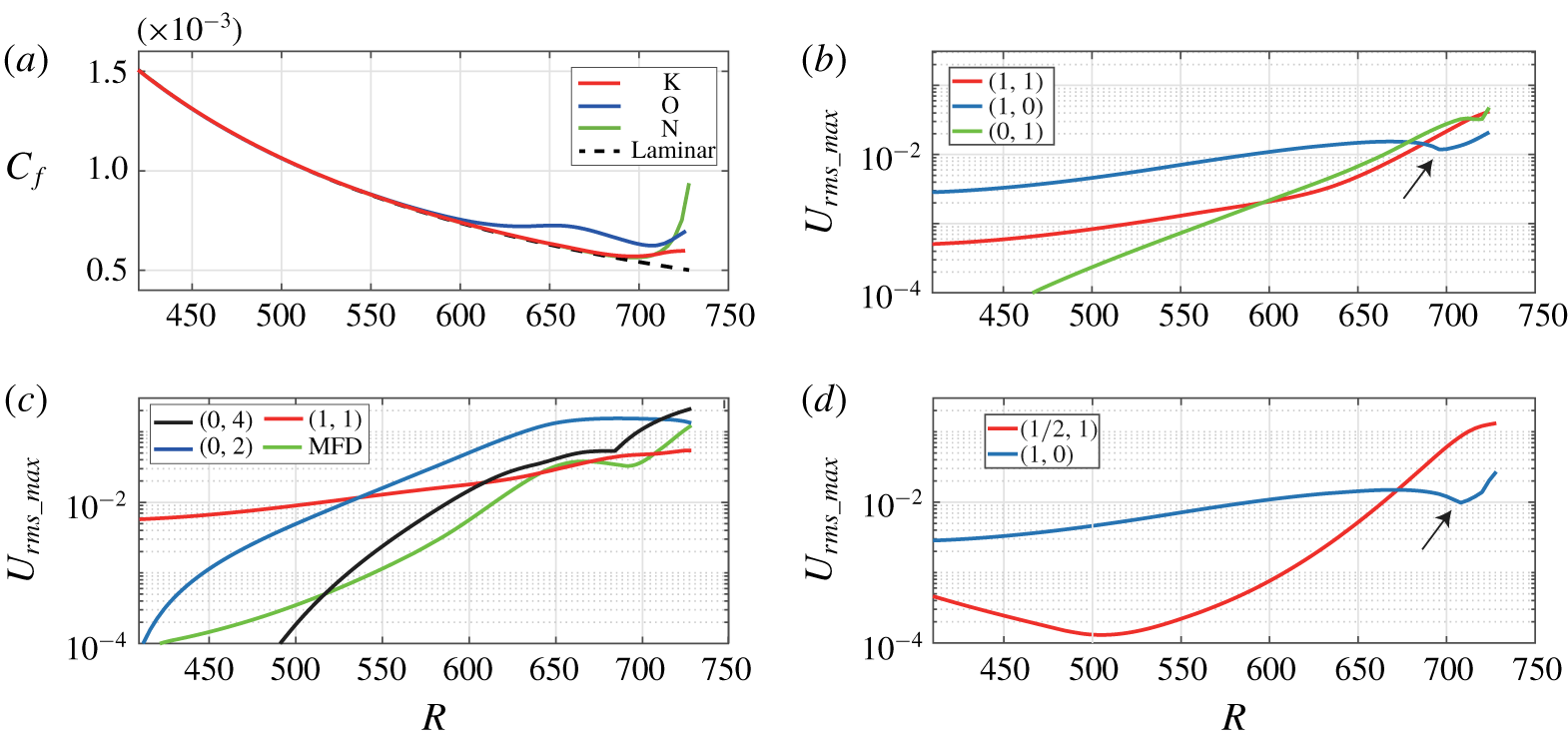
The downstream development of the averaged skin friction coefficient,  $C_{f}$, for the three transition regimes is shown in figure 1(a). The skin friction coefficient is calculated as
 $$\begin{eqnarray}C_{f}=\frac{2\bar{\unicode[STIX]{x1D707}}(\unicode[STIX]{x2202}\bar{u}/\unicode[STIX]{x2202}y)|_{y=0}}{R}.\end{eqnarray}$$
All the skin friction curves end at  $R=728$, where the NPSE becomes invalid. This position corresponds to
 $x=(R/R_{0})^{2}x_{0}=1325$, according to the normalization in § 2.1. The skin friction coefficient curves for the K- and N-regimes initially follow the laminar curve up to
 $R\approx 690$ (corresponding to
 $x\approx 1190$), then the curve for the K-regime increases slightly toward the end, while the curve for the N-regime rises steeply. The skin friction behaviour for the O-regime follows the laminar curve up to
 $R\approx 580$ (
 $x\approx 841$), then increases slightly up to
 $R\approx 660$ (
 $x\approx 1090$), where it begins to slowly decay. Beyond
 $R\approx 708$ (
 $x\approx 1253$), the curves rise again but more steeply than before. The initial departure of the skin friction coefficient from the laminar value, well before the final transition, is considered as the beginning of nonlinearity (Schmid & Henningson Reference Schmid and Henningson2001). These early nonlinear regions are what we focus in the preset study.
Skin friction coefficient  $C_{f}$ for the three transition regimes (a) and mode amplitude evolution for K-regime transition (b) O-regime transition (c) and N-regime transition (d). The arrows in (b,c) indicate a slight declination of the primary wave. The numbers in brackets denote normalized frequency–wavenumber as described in § 2.2 (table 1). MFD in (c) means mean-flow distortion.

As mentioned previously, Fourier mode decomposition is a basic method for investigating the transition behaviour. Thus, before presenting the structure-based results, it is helpful to examine the evolution of Fourier modes. Figure 1(c,d) shows the development of the  $y$-maxima of the selected Fourier amplitudes in the streamwise direction, for the K-, O- and N-regimes, respectively. The same language of normalized frequency–wavenumber as described in § 2.2 (table 1) is used here. Since the flow is symmetric for (
 $\unicode[STIX]{x1D714},\unicode[STIX]{x1D6FD}$) and (
 $\unicode[STIX]{x1D714},-\unicode[STIX]{x1D6FD}$), only the positive part is shown. For K-regime transition, figure 1(b), we determined that the transition is initiated by the growth of the amplitude of oblique modes (1, 1) and streak modes (0, 1), which successively surpass the amplitude of the fundamental disturbance (1, 0) at approximately
 $R=680$. Note that this is the location where the skin friction begins to deviate from the laminar curve in figure 1(a). The fundamental resonance between modes (1, 0), (1, 1) and (0, 1) has been considered as the main cause for initiating K-regime breakdown (Herbert Reference Herbert1988).
Figure 1(c) illustrates the evolution of four primary modes for O-regime transition. The modes (0, 2), (0, 4) and mean-flow distortion (MFD) mode (0, 0) are excited nonlinearly due to the interaction of modes (1,  $\pm 1$). After generation, the streak mode (0, 2) undergoes a transient growth stage due to a lift-up effect (Berlin, Lundbladh & Henningson Reference Berlin, Lundbladh and Henningson1994), and then becomes saturated for
 $R>650$. Mode (0, 4) also grows rapidly and becomes saturated driven by mode (0, 2) until
 $R\approx 670$, where it again begins to amplify, eventually surpassing the amplitude of mode (0, 2). The last growth of mode (0, 4) is probably due to a secondary instability of the streaks. The location where the mode (0, 4) surpasses the primary oblique mode is consistent with the location where the skin friction begins to deviate from its laminar value in figure 1(a). So, the first deviation of the skin friction curve is due to the growth of the streak mode, while the second deviation, which begins at
 $R\approx 708$, might be explained by the secondary instability of the streaks.
For N-regime transition in figure 1(d), during the amplification of the oblique mode, the primary wave undergoes a slight decrease, which is similar to the K-regime (see arrows in the figure). But the streak mode does not develop during the initial stage. Thus, the nonlinear amplification of the 3-D wave is mainly attributed to the growth of subharmonic oblique disturbances, which is consistent with previous results of experiments and DNS (Herbert Reference Herbert1997).
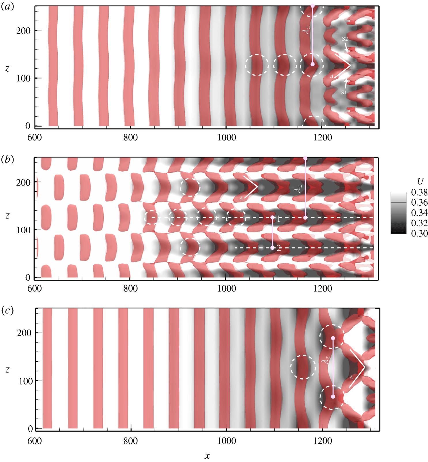
The development of Fourier amplitudes is closely related to the flow structure within the boundary layer. Figure 2(a–c) shows the contours of streamwise velocity (the grey contour) in the  $x$–
 $z$ plane at
 $y=2.5$, superimposed on iso-surfaces of positive second invariant of the velocity gradient, i.e.
 $Q$ value (the red region), for the transition of the K-, O- and N-regimes, respectively. Here,
 $Q=[|\unicode[STIX]{x1D734}|^{2}-|\unicode[STIX]{x1D64E}|^{2}]/2=0.00002~\text{s}^{-2}$, with
 $\unicode[STIX]{x1D734}=[\unicode[STIX]{x1D735}\boldsymbol{v}-(\unicode[STIX]{x1D735}\boldsymbol{v})^{\text{T}}]/2$ is the vorticity tensor, and
 $\unicode[STIX]{x1D64E}=[\unicode[STIX]{x1D735}\boldsymbol{v}+(\unicode[STIX]{x1D735}\boldsymbol{v})^{\text{T}}]/2$ is the rate-of-strain tensor (Hunt, Wray & Moin Reference Hunt, Wray and Moin1988). As shown in figure 2(a), the K-regime is characterized by aligned low-momentum zones (LMZ), the darker regions as indicated by dashed circles in the figure. These regions have a spanwise spacing of
 $\unicode[STIX]{x1D706}_{z}=125.66$, which is the same as the spanwise wavelength of the corresponding oblique waves (i.e.
 $2\unicode[STIX]{x03C0}/\unicode[STIX]{x1D6FD}=125.66$). The LMZs at far downstream locations are flanked by a pair of high-speed regions, labelled S1 and S2 in the figure. A 𝛬-vortex (‘ >’ in the figure) appears downstream of the location where the skin friction begins to deviate from the laminar curve (
 $x\approx 1190$).
Contour of streamwise velocity  $U$ (the grey shading) at
 $y=2.5$ and
 $t=0.8~\text{T}$, superimposed on iso-surfaces of
 $Q$-criterion detected structures (the red regions,
 $Q=0.00002~\text{s}^{-2}$). (a) K-regime transition; (b) O-regime transition; (c) N-regime transition. The flow is from left to right.

For the O-regime and N-regime, figure 2(b,c), the LMZs appear as staggered patterns. The staggered 3-D waves (dark regions within the dashed circles) for the O-regime develop nonlinearly from a pair of oblique waves (1,  $\pm 1$), appearing farther upstream than for the N-regime, with a spanwise wavelength of
 $\unicode[STIX]{x1D706}_{z}=125.66$. The streaks (the dashed lines) shown for the O-regime are spaced by
 $\unicode[STIX]{x1D706}_{z}/2=62.83$, as a result of the growing streak mode (0, 2). The low-speed streak (LSS), labelled 1 in figure 2(b), consists of several 3-D waves, indicated by the dashed circles along the streak. The 𝛬-vortices are observed to develop in conjunction with LSS regions, in a staggered pattern.
For the N-regime, figure 2(c), shows that the LMZs and 𝛬-vortices that develop well downstream are larger than those for the K- and O-regimes, since the streamwise wavelength of the amplified 3-D wave is twice that of the primary 2-D wave. No streak is observed in figure 2(c), which agrees with the development of mode amplitudes in figure 1(d). Because the 3-D waves appear prior to a 𝛬-vortex, as indicated by the position of the LMZs in the figure, a 𝛬-vortex is most likely produced by the nonlinear 3-D wave. It will be shown later that the 3-D waves are very similar to the soliton-like wave structure mentioned previously.
3.2 K-regime transition
3.2.1 Evolution of timelines and streaklines
K-regime timelines initiated at  $x=1011$,
 $y=1.71$, with
 $\text{d}t=12$. (a)
 $t=5.6T$; (b)
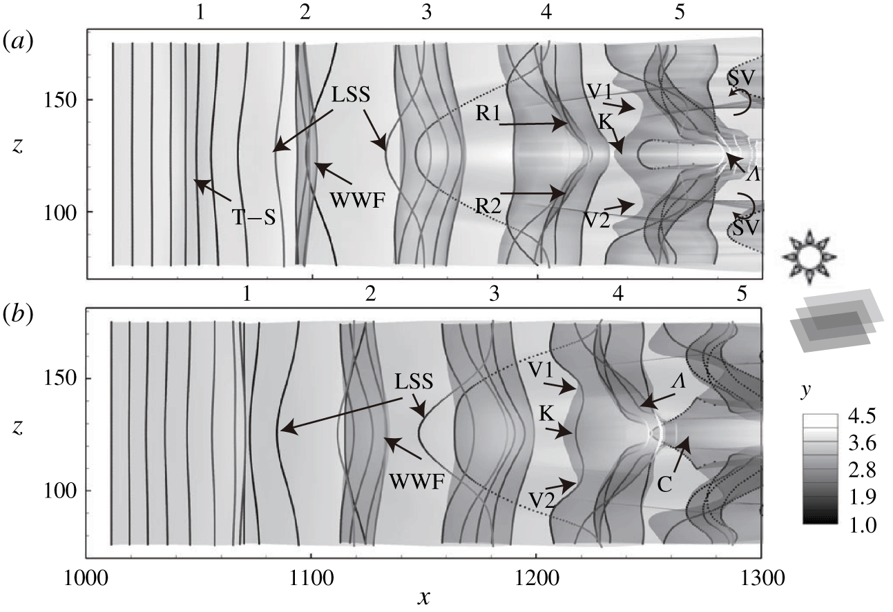
 $t=6.1T$. WWF, warped wave front; K, kink structure; R, roll-up; LSS, low-speed streak; C, chevron structure.

Figure 3 shows two snapshots of timelines initiated at  $y=1.71$ after development times of
 $t=5.6T$ and
 $6.1T$. Here,
 $T$ is the normalized time period of the primary wave defined in § 2.2. The timeline surface is displayed in greyscale, where the vertical location of the surface indicated by the scale to the right of the images (darker is nearer the wall, and lighter farther from the all). This represents a continuous timeline surface, similar to a timeline sheet formed by continuously releasing hydrogen bubbles. The translucency of the surface is set as 70 % to allow observation of the deformation of the timeline sheet. The volumetric rendering is sketched in the right schematic diagram. So, the shading in the figure shows the overlap of the surface, caused by the folding of the timeline surface. Figure 3(a) shows the deformation of the timeline sheet at
 $t=5.6T$, the behaviour of which is identified by a series of stages 1 to 5, showing the evolution from the initial T–S wave to a 𝛬-vortex. Figure 3(b) shows the spatial development of the timeline surface patterns at
 $t=6.1T$, a half-primary period later relative to figure 3(a). Figure 3 clearly shows how a 𝛬-vortex develops. Starting at stage 1, the 2-D T–S wave is distorted into a three-dimensional wave (3-D wave), with its wave front warped, indicated as a warped wave front – the wave front of a modulated two-dimensional wave that is strongly warped, as evidenced by the accumulation of times lines at stage 2. During stage 2, the WWF develops a fold in the timeline sheet and a low-speed streak appears, indicated by the retardation and downward motion of the timelines, labelled as LSS. By stage 3, the 3-D wave lifts up, with the WWF beginning to accelerate, leading to an initial roll-up of the wave front by stage 4 (see R1 and R2 in stage 4). This initial roll-up subsequently develops into an apparent 𝛬-vortex, at stage 5 in figure 3(a) and stage 4 in figure 3(b). The roll-up behaviour causes multiple folds of the surface, reflected by the darker shaded regions of the translucent sheet. During the folding process, streamwise depressions (V1 and V2) of the sheet toward the wall appear flanking the hairpin vortex, which subsequently develop into streamwise vortices, labelled SV in figure 3(a). Meanwhile, the kinked structure (labelled K), is observed to develop a chevron-shaped structure at a downstream position (labelled C). The details of the folding process are shown further in figures 4 and 5.
Plan view of the evolution of a single structure based on K-regime timelines (a,c,e,g,i) and a timeline surface (b,d,f,h,j) initiated at  $y=1.71$, with release interval
 $\text{d}t=0.2T$. (a,b)
 $t=5.1T$; (c,d)
 $t=5.6T$; (e,f)
 $t=6.1T$; (g,h)
 $t=6.6T$; (i,j)
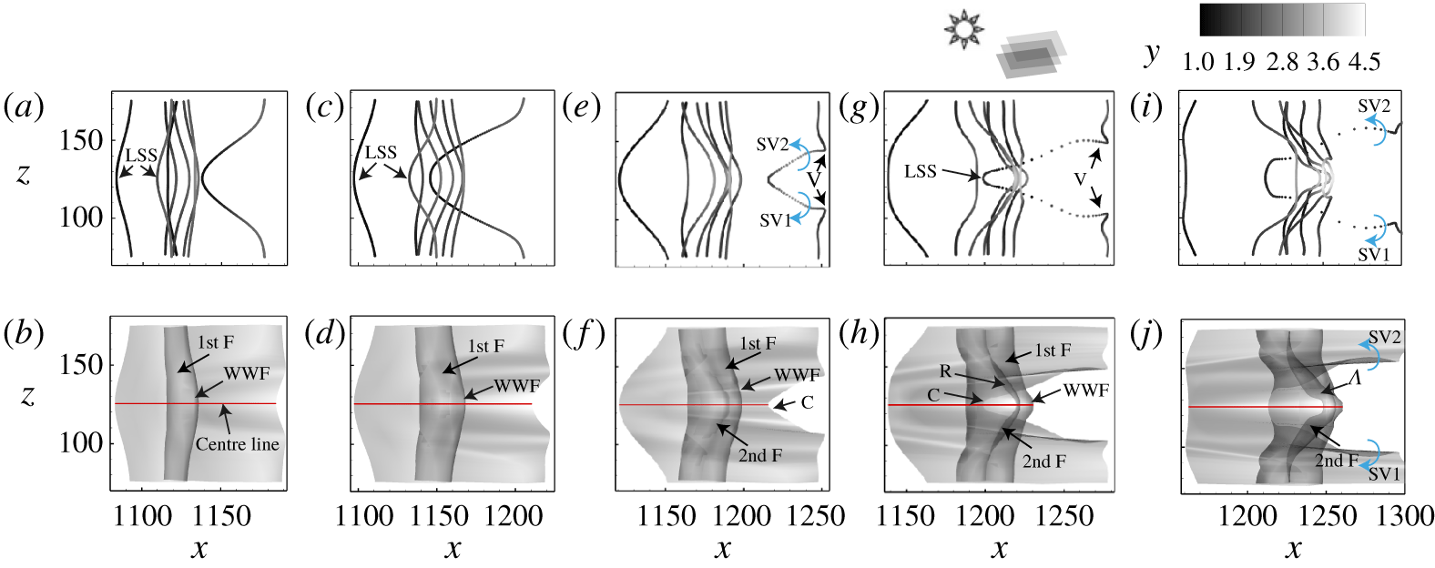
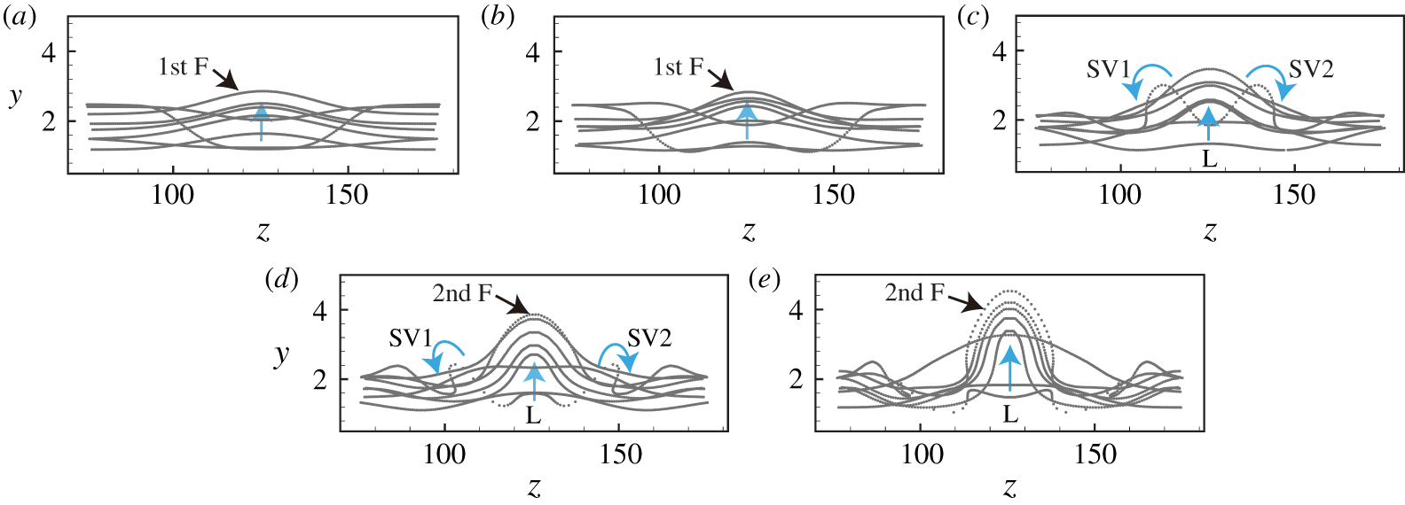
 $t=7.1T$. 1st F, first folding; 2nd F, second folding; SV, streamwise vortex. (See the supplementary Movie 1 for the complete evolution.)

End view of K-regime timelines (looking downstream) at the same time intervals as figure 4. (a)  $t=5.1T$; (b)
 $t=5.6T$; (c)
 $t=6.1T$; (d)
 $t=6.6T$; (e)
 $t=7.1T$. L, lift-up.

The first and second rows of figure 4 show the plan-view evolution of timelines and a timeline surface from  $t=5.1T$ to
 $7.1T$ at intervals of
 $0.5T$, corresponding to the structure shown initially as stage 3 in figure 3(a) (see the supplementary Movie 1, available at https://doi.org/10.1017/jfm.2020.107, for the complete evolution). The volumetric rendering for the surface is the same as figure 3. Figure 4(a,c) clearly shows a LSS with retarded timelines appearing below the WWF, which indicates that it is not the presence of a 𝛬-vortex that induces the low-speed streak pattern, but the lifting of the 3-D wave, since the 𝛬-vortex has not yet formed. The 3-D wave is initially reflected as a warping and accumulation of timelines, as shown in figure 4(a,c), or as a transverse fold in the timeline surface, as shown in figure 4(b,d). In figure 4(f), it is observed that the surface appears to develop a new fold (labelled 2nd F), which projects outward and above the portion of the surface marking the WWF. This second surface fold is more obvious at the later time of
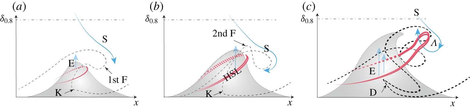
 $t=6.6T$, and will progressively develop into a 𝛬-vortex, as shown in figure 4(h,j). When a 𝛬-vortex appears, the timeline surface comprising the WWF begins to squeeze together and lift up, as the sequence of figure 4(e,g,i) shows. Previous studies assumed that the first folding (1st F) leads to the development of a 𝛬-vortex (Hama & Nutant Reference Hama and Nutant1963). However, figure 4 clearly demonstrates that a 𝛬-vortex develops from the second folding (2nd F) of the wave front. The lifting of the 3-D wave deforms the 2-D timelines, and causes the first and second foldings. It should be noted that the chevron-like structure, labelled C in figure 4(f,h), is actually a reflection of the low-speed streak developing near the wall along the centre line (red line in the figure). The two high-speed valleys (V1, V2) that were previously identified in figure 3, which flank the chevron-like structure (C), are shown in figure 4(h,j) to develop into rotational streamwise vortices (SV1, SV2). Note that the above warping process is unobservable when the timelines are initiated at a higher position such as
 $y=3.83$. In that case, the evolution of three-dimensional wave is obvious, see the supplementary Movie 2 for the complete evolution.
Figure 5 shows the corresponding end views of the five timeline patterns shown in figure 4(a,c,e,g,i). These end-view patterns clearly demonstrate the lift-up (labelled L in the figures) of a 3-D wave. Note that figure 5(d,e) shows that the second folding of the timelines protrudes above the first folding, which develops into the head of a 𝛬-vortex. The development of the two streamwise vortices is also clearly shown in figure 5(c,d), labelled SV1 and SV2 flanking the sides of the lifted WWF.
Side view of vertical timelines initiated at  $z=126$ (near centre plane) for K-regime transition, with release intervals
 $\text{d}t=0.16T$. (a)
 $t=2T$; (b)
 $t=3T$; (c)
 $t=4T$; (d)
 $t=5T$. The wavelength
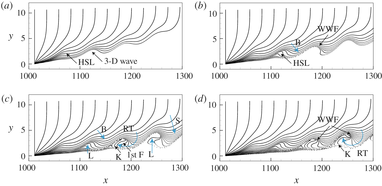
 $\unicode[STIX]{x1D706}\approx 52.7$. HSL, high-shear layer; W, 3-D wave; B, wave front leading edge; RT, rotation; S, downward sweep. See the supplementary Movie 7 for the complete evolution.

The breakdown of a wave motion into hairpin eddies has been demonstrated to be a consequence of the instability arising from three-dimensional wave behaviour (Klebanoff et al. Reference Klebanoff, Tidstrom and Sargent1962). Klebanoff suggested the instability was similar to a secondary inflectional instability. The results of the present investigation also indicate that the 𝛬-vortex develops from a 3-D wave-induced inflectional instability. Figure 6 shows the evolution of vertical timelines initiated at  $z=126$ (near the centre plane shown as red line in figure 4), with release intervals of
 $\text{d}t=0.16T$. The streamwise extent shown for the
 $x$-direction is almost
 $5.5\unicode[STIX]{x1D706}$, where
 $\unicode[STIX]{x1D706}$ is the wavelength of the primary T–S wave. The instantaneous velocity profiles at
 $t=2T$,
 $3T$,
 $4T$,
 $5T$ are markedly similar to those shown by Hama & Nutant (Reference Hama and Nutant1963) using hydrogen bubble timelines. As shown in figure 6(a), an inflectional high-shear layer (HSL) develops as the 3-D wave lifts up. This is followed by the development of a warped wave front, as shown in figure 6(b). Figure 6(c) shows that the WWF undergoes further stretching and develops the first folding of timelines (1st F), with the kink structure (K) also developing during the folding process. The leading edge (B) of a WWF creates a strong downward sweep (S) as transition proceeds. Finally, as shown in figure 6(d), rotation (RT) of the WWF progressively evolves into the head of a 𝛬-vortex, which results in the entrainment of higher-speed outer flow into the 𝛬-vortex and toward the wall.
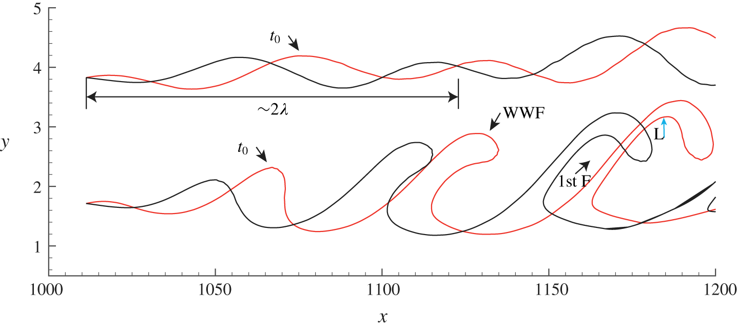
Figure 7 shows streaklines initiated at both  $y=1.71$ and 3.83 near the centre plane (
 $z=126$), which illustrate the amplification and evolution of the wave behaviour. The streakline initiated at
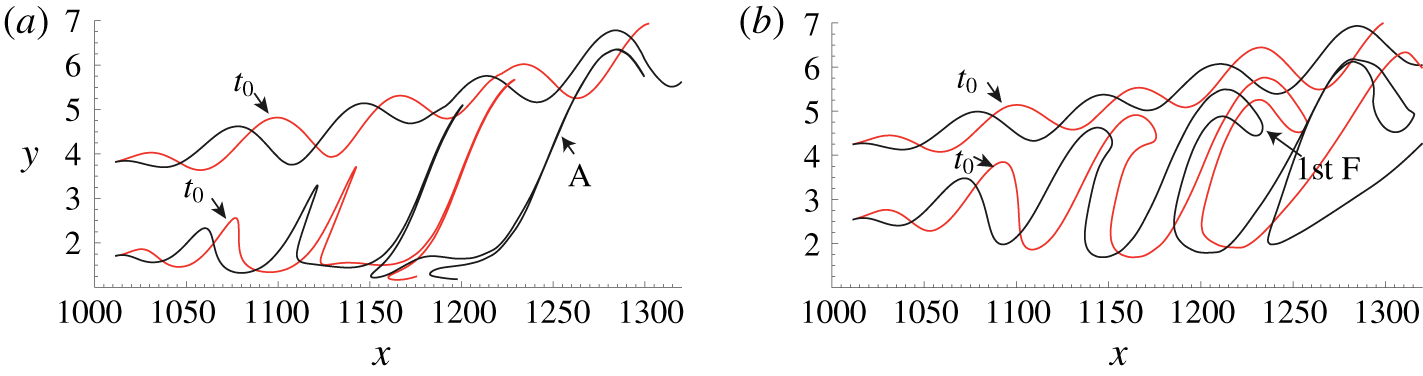
 $y=1.71$ clearly shows the first folding process of the WWF. The wave front undergoes a rotational behaviour downstream similar to those shown by Kelvin–Helmholtz waves or Holmboe waves (Smyth & Peltier Reference Smyth and Peltier1991; Lefauve et al. Reference Lefauve, Partridge, Zhou, Dalziel, Caulfield and Linden2018). However, the upper streakline, initiated higher at
 $y=3.83$, only undergoes a modest wave amplification. Two factors are considered to be relevant to the different wave behaviour: the first is the shear strength, and the second is the amplitude of the 3-D disturbance. Note that the upper streakline seems to behave as a superposition of the primary wave and its subharmonic, indicated by the wavelength of
 $2\unicode[STIX]{x1D706}$ on the figure. As pointed out by Kachanov (Reference Kachanov1994), subharmonic resonances are also important in K-regime transition, and the streakline behaviour of figure 7 may be a reflection of the development of subharmonic resonance.
Evolution of K-regime streaklines initiated at  $y=1.71$ and 3.83 on the plane of
 $z=126$: red line for
 $t_{0}=4T$; black line for
 $t_{0}+0.72T$.

3.2.2 Evolution of material surfaces
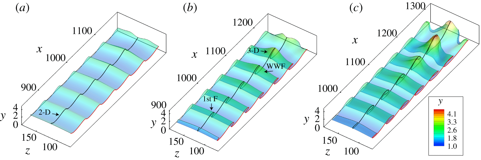
Figure 8 shows the evolution of an initially flat material surface ( $\unicode[STIX]{x0394}z=98$,
 $\unicode[STIX]{x0394}x=316$) initiated at
 $y=1.71$ and
 $x_{initial}=800\sim 1116$. The deformation of the material surface from
 $1T$ to
 $3T$ shown in figure 8(a–c) is similar to that of the timeline surface shown in figure 3. Figure 8(a) illustrates a stage where the 2-D wave has undergone a weak 3-D deformation, with its crest inclined slightly downstream. As the wave amplifies, figure 8(b) shows that the inclined 2-D wave undergoes strong spanwise deformation, developing a three-dimensional WWF. This WWF is the typical first folding stage. Figure 8(c) shows that the WWF continues to deform three-dimensionally, and gradually evolves into a 𝛬-vortex. A black material line along the centreline of the wave amplification process illustrates the same folding behaviour as illustrated by the timelines and streaklines of figures 4 and 6.
Evolution of a material surface initiated at  $y=1.71$ for K-regime transition. (a)
 $t=1T$; (b)
 $t=2T$; (c)
 $t=3T$. Note that the wall-normal coordinate scale is 10 times magnified.

3.3 O-regime and N-regime transition
The evolution of a single structure based on O-regime timelines initiated at  $y=1.71$, with release interval
 $\text{d}t=0.3T$. (a,d,g,j,m) End view of timelines; (b,e,h,k,n) plan view of timelines; (c,f,i,l,o) plan view of a rendered timeline surface. (a–c)
 $t=4T$; (d–f)
 $t=5T$; (g–i)
 $t=6T$; (j–l)
 $t=7T$; (m–o)
 $t=8T$. (See the supplementary Movie 3 for the complete evolution.)

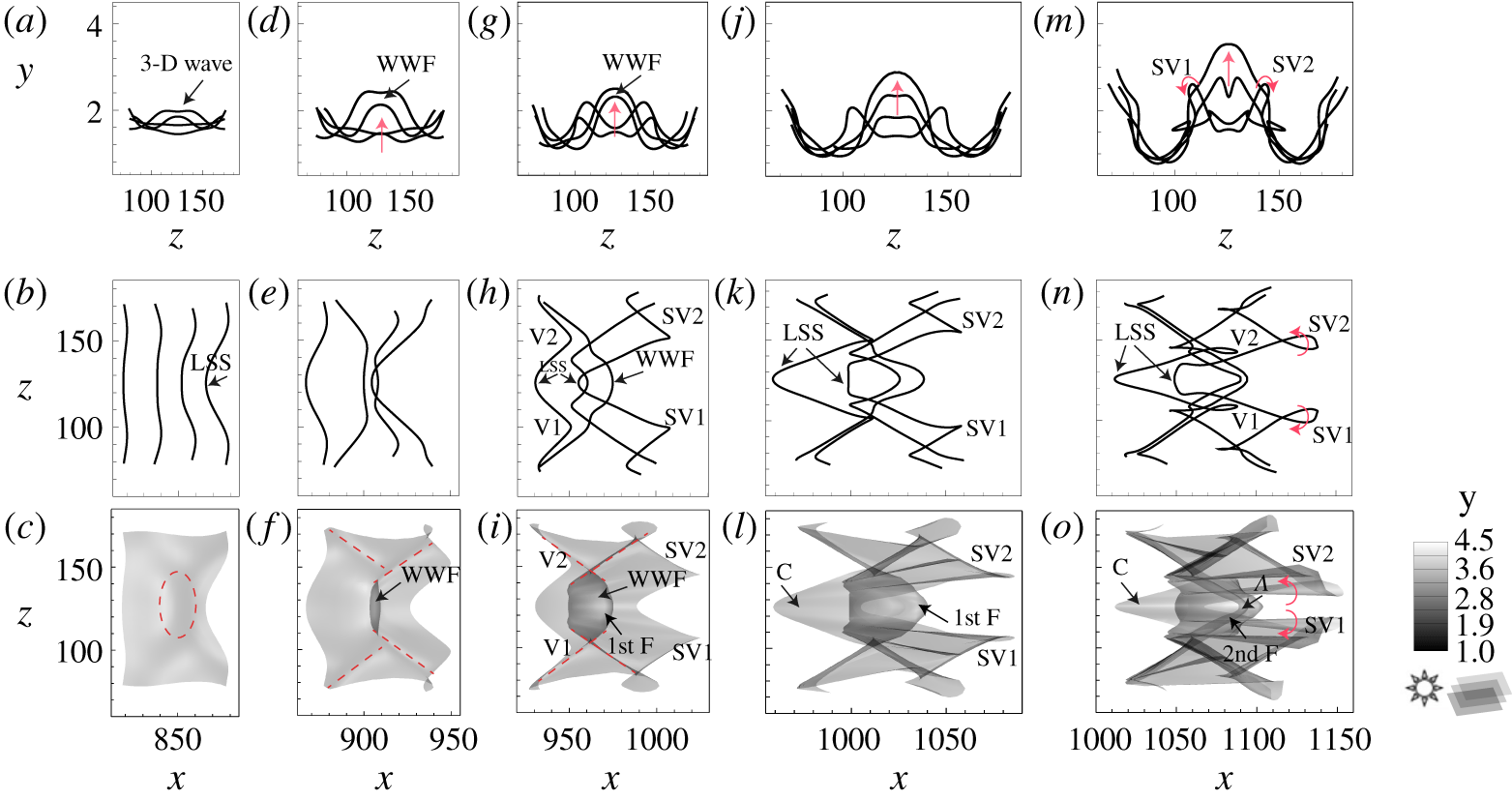
The evolution of a single structure based on timelines generated for the O-regime is shown in figure 9. (See the supplementary Movie 3 for the complete evolution of how a 3-D wave develops into a 𝛬-vortex in O-regime transition.) Figure 9(a,d,g,j,m) shows end views of five timeline patterns from  $t=4T$ to
 $8T$. Similar to the patterns shown in figure 5 for the K-regime, the 3-D wave is initially very weak, figure 9(a), but then develops into a WWF and expands in both the normal and spanwise directions, moving progressively upward. Some instability occurs adjacent to the two sides of the WWF, as illustrated by the intertwining timelines in figure 9(m). figures 9(b,e,h,k,n) and 9(c,f,i,l,o) show the corresponding plan view of the development of a 𝛬-vortex in O-regime transition, both for individual timeline behaviour (b,e,h,k,n) and as a developing timeline surface (c,f,i,l,o). First, the interaction of oblique waves produces a 3-D wave, manifested as weakly retarded timelines (LSS) or a small bulge (red dashed circle), figure 9(b,c). Next, the lift-up of the 3-D wave produces a warped wave front, with rhombic creases appearing on the timeline surface, as indicated by the red dashed lines in figure 9(f). The first folding (1st F) of the surface strengthens the creases (red dashed lines) that flank the WWF, figure 9(i). During the strengthening process, regions of apparent depression (labelled V1, V2, SV1, SV2) form, similar to those shown in figure 3. Subsequently, a chevron-like structure (C) develops below the WWF, constituting a more confined LSS, as shown in figure 9(k,l). Finally, the second folding develops on the timeline surface to form a 𝛬-vortex, during which the previous rhombic creases begin to rotate, developing streamwise vortices from the initial regions of depression, figure 9(n,o). Note that the above multi-folding process is not discernible when the timelines are initiated at
 $y=3.83$. In that case, the evolution of three-dimensional wave is clearly observed, which seems to constitute a low-speed streak (see the supplementary Movie 4 for the complete evolution).
The evolution of a single structure based on N-regime timelines initiated at  $y=1.71$, with release interval
 $\text{d}t=0.3T$. (a,d,g,j,m) End view of timelines; (b,e,h,k,n) plan view of timelines; (c,f,i,l,o) plan view of rendered timeline surface. (a–c)
 $t=5.1T$; (d–f)
 $t=6.4T$; (g–i)
 $t=7T$; (j–l)
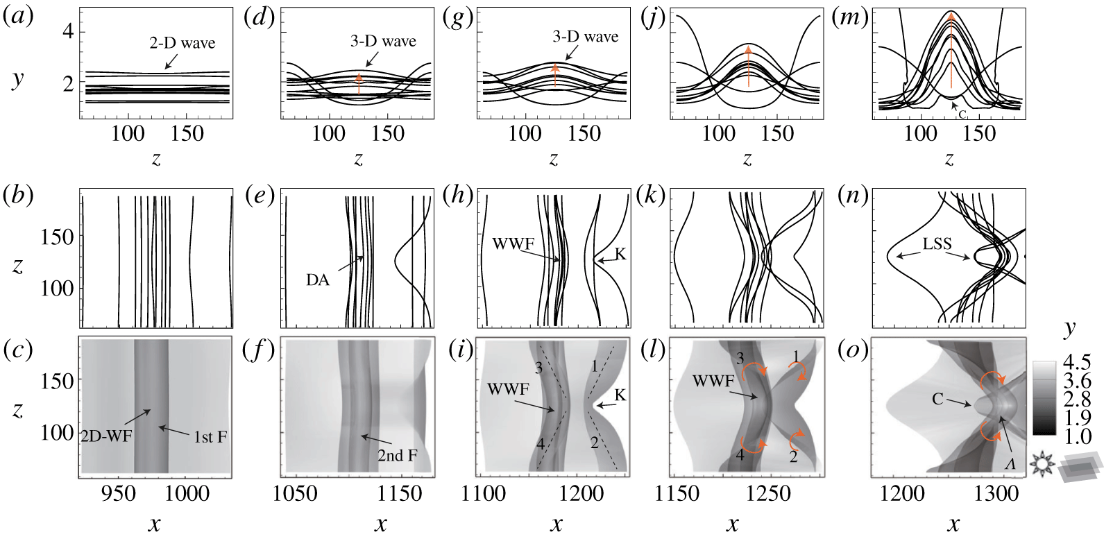
 $t=7.5T$; (m–o)
 $t=8T$.

Figure 10, similar to the presentation in figure 9, shows the evolution of a single structure developing from a 2-D T–S wave into a 𝛬-vortex for the N-regime (see the supplementary Movie 5 for the complete evolution). The end-view timelines (upper row) demonstrate lift-up behaviour similar to the K- and O-regimes, but no apparent streamwise vortex develops, unlike those apparent shown in figures 5 and 9 (labelled SV1 and SV2). As shown in figures 10(b,e,h,k,n) and 10(c,f,i,l,o), during the lift-up process, a two-dimensional wave front (2D-WF) gradually evolves into a three-dimensional warped wave front (WWF), from  $t=5.1\sim 7T$, which subsequently develops into a 𝛬-vortex; this process is illustrated most clearly by figure 10(c,f,i,l,o). The development process looks markedly similar to those shown by Hama & Nutant (Reference Hama and Nutant1963). The wave front is initially two-dimensional (see 2D-WF), as shown by the 2-D timelines in figure 10(a), with the transverse folding of the timeline surface (1st F) developing in figure 10(c). As time progresses, the second folding develops, figure 10(d,f), which corresponds to a denser accumulation of timelines indicated by DA in figure 10(e), which differs from K- and O-regime transition. When the warping of the wave front takes place (regions labelled 3 and 4 in figure 10i), a WWF develops, accompanied by retarded regions (labelled 1 and 2) preceding the WWF. As the warping progresses, the timelines coalesce and deform to form the head of a 𝛬-vortex, with upward motion of the WWF intensifying, figure 10(j–l). The rotation and coalescence of the timelines along what appears as a swept-back region (regions labelled 1, 2, 3, 4 in figure 10l) indicate that vorticity is concentrated along the swept-back sides. Eventually, a 𝛬-vortex develops and is strengthened due to streamwise stretching, with red arrows indicating the rotation of the swept-back legs in figure 10(o). The retarded region indicated by K in figure 10(i), is shown in figure 10(o) to have evolved into a chevron-shaped structure (labelled C) beneath the 𝛬-vortex, and appears to be a localized LSS, as shown in figure 10(n). Note also that the WWF and its warping process is indiscernible when the timelines are initiated at
 $y=3.83$ (see the supplementary Movie 6 for the complete evolution).
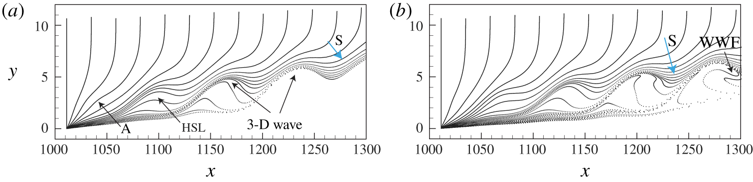
Vertical timelines of O-regime transition at (a)  $t=3T$ and (b)
 $t=4.6T$, initiated near the centre plane
 $z=126$. (See the supplementary Movie 7 for the complete evolution.)

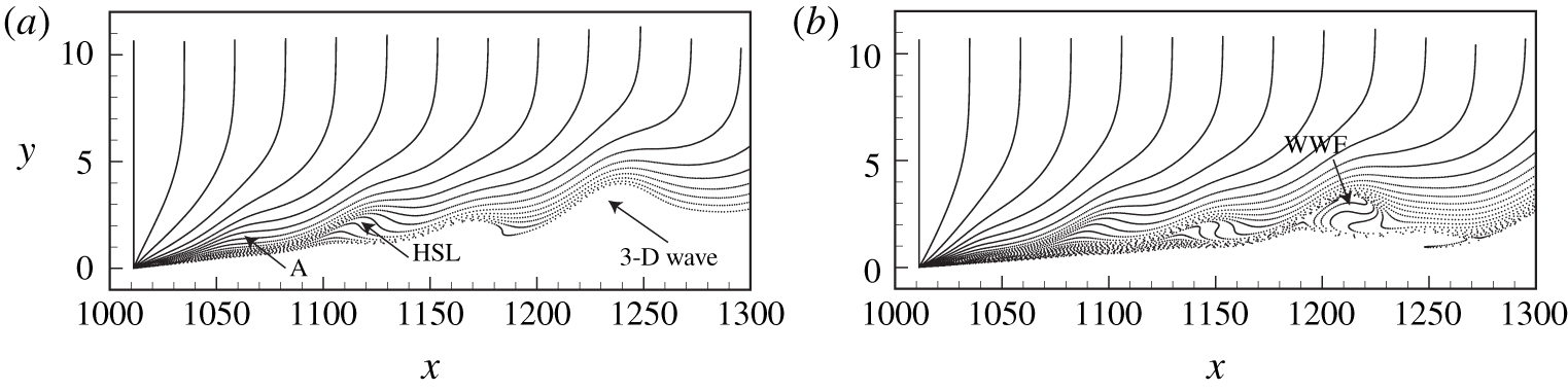
Vertical timelines of N-regime transition at (a)  $t=3T$ and (b)
 $t=4.6T$, initiated near the centre plane
 $z=126$. (See the supplementary Movie 7 for the complete evolution.)

The vertical timeline patterns for the O-type and N-type regimes are shown in figures 11 and 12. These profiles are initiated at  $x=1011$ and
 $z=1256$ (the centre plane), with release intervals
 $\text{d}t=0.2T$. Figures 11 and 12 show patterns similar to figure 6 for the K-regime. In both these figures, an inflectional region (A) develops in the near-wall region of the profiles, which progressively develops a humplike pattern, implying an HSL, and created by a lifting 3-D wave. The leading edge of this humplike pattern subsequently precipitates a strong downward sweep (S), and evolves into a warped wave front, which will further develop into a transverse rotational pattern as the head of a 𝛬-vortex. The humplike structure observed here corresponds to what is described by Hama & Nutant (Reference Hama and Nutant1963) as a ‘kink’ structure, whose breakdown was considered to be responsible for the formation of discrete vortices. Note that this process of development of the hump-like kink pattern for the N-regime occurs closer to the wall than for the K- and O-regimes, as illustrated by a comparison of figure 12 with figures 6 and 11, with the size of the hump-like patterns for the N-regime appearing smaller (see the supplementary Movie 7 for the comparison between the three regimes).
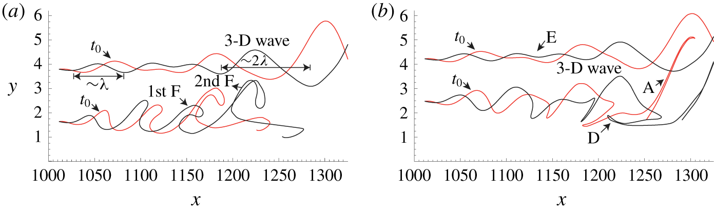
Figures 13 and 14 show the evolution of streaklines for both O-regime and N-regime transitions. The streaklines are initiated at four different wall-normal positions, i.e.  $y_{0}=1.71$, 2.54, 3.83 and 4.25, and show streakline patterns for two different development periods. For the O-regime, the streaklines at the near-wall position
 $y_{0}=1.71$ are stretched into a thin filament projecting strongly into the outer layer (labelled A in the figure), indicating a severe wave deformation. When compared with patterns shown in figure 9, the location of the thin, stretched filament is consistent with the location where a 𝛬-vortex develops. However, note that comparably strong wave deformation does not occur for the streaklines initiated at
 $y_{0}=3.83$ and 4.25, which behave essentially as a modest wave-like amplification. The streakline initiated at
 $y_{0}=2.54$ in figure 13(b) shows the development of the first folding of the wave front, which is striking in its similarity to the streakline behaviour for the K-regime transition, generated at
 $y_{0}=1.71$ (figure 7).
Evolution of streaklines for O-regime transition initiated at different wall-normal positions  $y_{0}$. (a)
 $y_{0}=1.71$ and 3.83; (b)
 $y_{0}=2.54$ and 4.25.
 $t_{0}=4T$ (red),
 $t_{1}=4.72T$ (black).

Evolution of streaklines for N-regime transition initiated at different wall-normal positions  $y_{0}$. (a)
 $y_{0}=1.71$ and 3.83; (b)
 $y_{0}=2.54$ and 4.25.
 $t_{0}=4T$ (red),
 $t_{1}=4.72T$ (black).

For N-regime transition, shown in figure 14, the streaklines initiated at the upper locations also reflect a modest wave-like amplification similar to the O-regime, although they do not move outward and appear more amplified than for the O-regime of figure 13. The waveform shows a superposition of the primary wave (of wavelength of  $\unicode[STIX]{x1D706}$) and its subharmonic (of wavelength of
 $2\unicode[STIX]{x1D706}$), similar to the K-regime behaviour in figure 7. As shown by the streaklines initiated at
 $y_{0}=3.83$ and 4.25 in figure 14, the subharmonic wavelength (
 $2\unicode[STIX]{x1D706}$) is strongly amplified downstream and becomes the dominant wavelength. This amplification may be a reflection of typical subharmonic resonance. Note that prior to the strong amplification to a 3-D wave, there appears to be a relatively quiet zone, labelled E in figure 14(b). The presence of this quiet zone is hypothesized to be the result of a nonlinear interaction between waves, i.e. the attenuation of the primary wave (
 $\unicode[STIX]{x1D706}$) and the growth of a low-frequency disturbance (at nearly
 $2\unicode[STIX]{x1D706}$). Indeed, the location of the quiet zone is identical to the position of the attenuation of the primary wave shown in figure 1(d); clearly, the mechanism for development of this quiet zone merits further study.
The streakline initiated at  $y_{0}=1.71$, figure 14(a), displays a similar warping process (a 1st folding and 2nd folding) to the K- and O-regimes. The streakline initiated at
 $y_{0}=2.54$, figure 14(b), again displays a strongly stretched, thin filament (labelled A), which is also observed in the region where a 𝛬-vortex appears (
 $x=1250{-}1300$). A backward stretched filament (labelled D) at the bottom of the 3-D wave front is slightly lifted up away from the wall, which appears coincident with the chevron-like pattern (C) in figure 10. The projecting thin filament pattern, which develops at the downstream warped wave front, is only observed for streaklines initiated close to the wall for all regimes. The results of figures 13 and 14 illustrate that the amplitude of the 3-D wave decreases with distance from the wall, and that the lift-up of the 3-D wave is much stronger in the near-wall region. Note that the evolution of streaklines for N-regime transition is markedly similar to the simulation of streaklines in a 2-D shear layer perturbed by one or two travelling waves (Hama Reference Hama1962; Williams & Hama Reference Williams and Hama1980), although no second folding behaviour was observed in those studies.
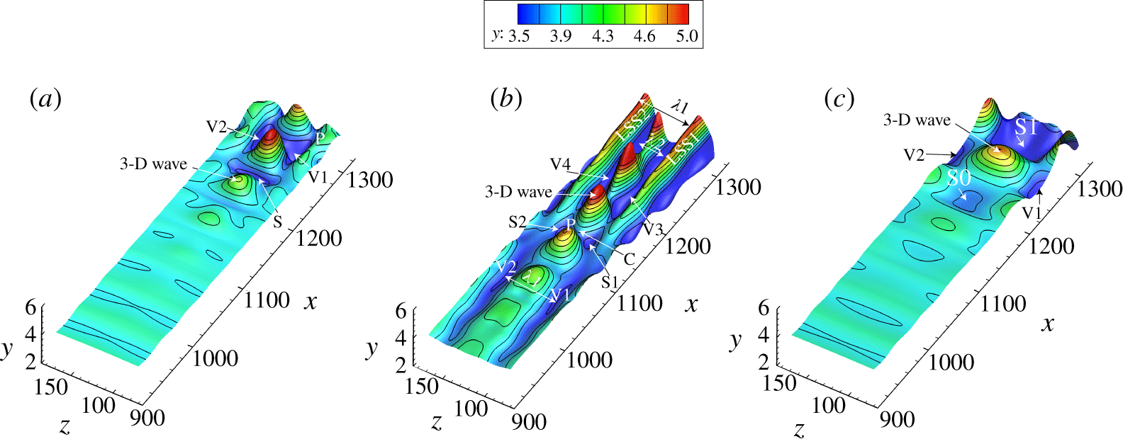
Material surfaces at  $t=1T$, initiated at
 $x_{initial}=795\sim 1309$,
 $z_{initial}=77\sim 175$,
 $y_{0}=3.83$. (a) K-regime transition; (b) O-regime transition; (c) N-regime transition.

Figure 15 shows the deformation of an initially flat material surface ( $x_{initial}=795{-}1309$,
 $z_{initial}=77{-}175$) initiated at
 $y=3.83$, for the three transition regimes at
 $t=1T$. The black contour lines illustrate respective changes in
 $y$ height, and show the development and growth of three-dimensional waves. Figure 15(a) shows that for the K-regime, an upstream 2-D wave progressively amplifies into an apparent 3-D wave, appearing at approximately
 $x\approx 1200$. This 3-D wave subsequently amplifies with its wave front (P) lifting up. At the front of the 3-D wave, there is a region of depression labelled S, which may be the result of a downward sweep event. As the 3-D wave develops downstream, this region of depression evolves into two regions (labelled V1, V2) flanking both sides of the rising 3-D wave. Note that the wave front at this position does not undergo as severe a warping as shown in figure 8, which was for a material sheet initiated much closer to the wall.
For O-regime transition, figure 15(b) shows that a rising 3-D wave (labelled P) develops much sooner than the K-regime, which is also accompanied by regions of depression (labelled S1 and S2). However, figure 15(b) shows the development of four longitudinal depressions or valleys (labelled V1, V2, V3, V4) flanking the sides of the 3-D wave fronts, which is markedly different from figure 15(a). These valleys span several wavelengths of the 3-D wave in the streamwise direction. For the K-regime of figure 15(a), the spacing ( $\unicode[STIX]{x1D706}_{1}$) between the valleys V1 and V2 is approximately
 $1/2\unicode[STIX]{x1D706}_{z}$, where the
 $\unicode[STIX]{x1D706}_{z}$ is the spanwise wavelength of the introduced oblique waves. However, the spacing (
 $\unicode[STIX]{x1D706}_{2}$) between valleys V3 and V4 in figure 15(b) for the O-regime is approximately half that of V1 and V2, i.e.
 $1/4\unicode[STIX]{x1D706}_{z}$. Two longitudinal streaks (LSS1 and LSS2) are observed outside the valleys V3 and V4, which are also spaced at approximately
 $\unicode[STIX]{x1D706}_{1}$, similar to the spacing between V1 and V2. These streaks are identified as low-speed streaks (LSS), which are a result of low-speed fluid moving upwards due to some type of uplift event.
Figure 15(c) shows the deformation of the material surface for N-regime transition, which looks similar to the K-regime, except that the dimensions of the 3-D wave are larger, and the 3-D waves develop later in the transition process. Regions of depression labelled V1, V2 and S0, S1 surround the 3-D wave, forming a staggered pattern. No longitudinal streaks or valleys are observed at this point of development for the N-regime.
In the present section, ‘kernel’ studies of both the O- and N-regimes followed the evolution of a 3-D wave into a 𝛬-vortex. These studies were facilitated using spatial-temporal visualizations of synthetic multi-perspective timelines, streaklines and material surfaces initiated at different heights and amplification periods. The results of O- and N-regime transition are compared to those of K-regime shown in § 3.2, and the similarities of WWF and its warping process are pointed out. A mutual comparison of the deformation of material surfaces for all three regimes, illustrates a similar pattern of 3-D wave development in the transition process.
4 Comparison with experiments
4.1 Description of the experiments
4.1.1 Facility and model
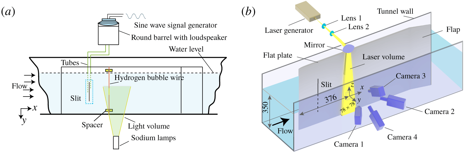
The experiments were performed in the PWT (Peking University Water Tunnel), an open-surface recirculating water channel with a cross-section of  $0.4~\text{m}\times 0.4~\text{m}$ and length of 6 m. The tunnel free-stream velocity range is 0.1 to
 $1.3~\text{m}~\text{s}^{-1}$, with a turbulence level of 0.77 % at the velocity of
 $0.17~\text{m}~\text{s}^{-1}$. For simplicity, only experiments of K-regime transition were done because it was easier to assure that the flow behaviour was comparable to prior studies at Peking University (Lee & Li Reference Lee and Li2007). The flat plate and disturbance generator were the same as those used by Lee & Li (Reference Lee and Li2007), which had been verified to be effective in producing T–S wave and K-regime transition. The flat plate test section, shown in figure 16(a), has a length of 1.8 m, a span of 0.8 m and a thickness of 15 mm. The flat plate was mounted vertically on the centreline of the tunnel at zero angle of attack, with an adjustable flap mounted at the trailing edge. The organized perturbations for the developing laminar boundary layer were generated using periodic suction and blowing at the wall, through a spanwise wall slit, 150 mm by 1 mm, located on the working side of the plate, 200 mm from the leading edge. As shown in figure 16(a), a loudspeaker mounted on the top of a water tank generated a controlled 2 Hz sinusoidal (via a signal generator) fluid injection–suction pattern from the slit via a tube connected from the water tank to a plenum behind the slit. The amplitude of the forced disturbance was approximately
 $1.1\,\%\,U_{\infty }$.
4.1.2 Experimental techniques and data acquisition
A series of hydrogen bubble timeline visualizations were done employing horizontal-wire configurations as described by Lee & Li (Reference Lee and Li2007), see figure 16(a). The hydrogen bubble wire was 0.03 mm diameter platinum wire. The distance of the wire from the plate surface was adjusted using insulated, calibrated spacers between the wire and the plate. By pulsing the current through the hydrogen bubble wire at a constant frequency, a pattern of timelines is created. If the current to the wire is kept constant, a continuous bubble sheet will be generated. The free-stream velocity for all studies was approximately  $0.17~\text{m}~\text{s}^{-1}$, and the distance,
 $x_{d}$, from leading edge to the centre of the tomo-PIV measurement region was 376 mm.
Experimental set-up of tomo-PIV: (a) plan view of set-up for hydrogen bubble visualization; (b) schematic layout of the arrangement of the tomo-PIV system.

The tomo-PIV configuration is shown in figure 16(b). Four high-speed CMOS cameras (Photron FASTCAM SA4) with resolution of  $1024\times 1024$ pixels at framing rates up to 3600 f.p.s. were used, in a cross-configuration arrangement. The cameras are fitted with Nikon lenses of 200 mm focal length at an aperture setting of
 $f/11$. Illumination was provided by a DCQ-30Q, high-speed laser generator from Beijing ZK Laser. The thickness of the light volume is 30 mm. The four cameras and laser system were controlled by Davis 8.4 software, and were synchronized using a LaVision PTU timing controller. Hollow glass particles, with mean diameter
 $11~\unicode[STIX]{x03BC}\text{m}$, were introduced into the water tunnel 6 m downstream of the test section to assure that the particles were fully mixed and uniformly distributed after circulating to the measurement site. Experiments were conducted at a particle image density of 0.098 particles per pixel, which corresponds to particle concentrations of approximately
 $2.3~\text{particles}~\text{mm}^{-3}$.
The tomo-PIV sampling frequency was 500 Hz, with a maximum sampling time of 20 s. The final residual calibration errors for all cameras was less than 0.1 pixel. The calibration field of view had a digital resolution of  $74.80~\unicode[STIX]{x03BC}\text{m}$ per pixel. The measurement domain extended 78 mm in the streamwise direction and 78 mm in the spanwise direction. Volume self-calibration (Wieneke 2008) was used on the pre-processed particle images. Sequential motion tracking enhancement (SMTE, Lynch & Scarano Reference Lynch and Scarano2015) was applied to volume reconstruction. The reconstructed volume was
 $1041\times 1048\times 187$ voxels. A multi-pass approach of four steps was carried out for the volume correlation, and the interrogation volume size for the final pass was
 $16\times 16\times 16$ voxels (
 $1.2\times 1.2\times 1.2~\text{mm}^{3}$) with a 75 % overlap. As a final step, a Gaussian smoothing filter of
 $3\times 3\times 3$ subvolume was applied to the velocity data. Proper orthogonal decomposition (POD) analysis has shown to be effective for noise removal and extraction of high modes in turbulent flow (Moin & Moser Reference Moin and Moser1989; Hellström & Smits Reference Hellström and Smits2017). In the present paper, POD analysis was applied to the smoothed velocity data sets, and the first four leading-order POD modes are extracted, in accordance with the methods of Zhu et al. (Reference Zhu, Wang, Wang and Wang2017). The POD approximated vector fields are the data sets used in the following postprocessing and analyses.
4.1.3 Properties of the boundary layers and PIV accuracy
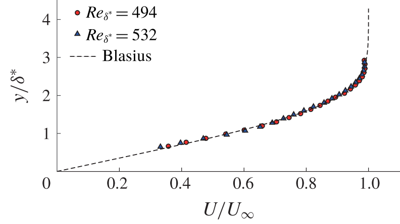
Measurements of two boundary-layer profiles compared with the Blasius profile.

Characteristic boundary-layer parameters and resolution parameters of tomo-PIV measurements:  $Re_{\unicode[STIX]{x1D703}}$ is the momentum-thickness-based Reynolds number;
 $\unicode[STIX]{x1D6FF}_{\unicode[STIX]{x1D703}}$ is the momentum thickness and
 $\unicode[STIX]{x1D6FF}^{\ast }$ is the displacement thickness;
 $H$ is the shape factor.

The spanwise averaged boundary-layer velocity profiles at two streamwise positions, obtained from the tomo-PIV data sets, are shown in figure 17 compared with a conventional Blasius profile (White Reference White2006). The wall-normal coordinate is scaled on the displacement thickness  $\unicode[STIX]{x1D6FF}^{\ast }$ of the laminar boundary layer, and shows that the averaged velocities agree well with the Blasius profile. Table 2 summarizes the characteristic parameters for the initial laminar boundary layer. Table 2 also lists the space and time resolution of the PIV data. The tomo-PIV measurements in this study provided velocity information on a grid of
 $0.3\times 0.3\times 0.3~\text{mm}^{3}$ over the volume of
 $78\times 78\times 30~\text{mm}^{3}$; the sample time increments are
 $\unicode[STIX]{x0394}t=0.002~\text{s}$. The turbulence intensity of the free stream measured by tomo-PIV is
 $0.0077U_{\infty }$, which suggests that the root-mean-square (r.m.s.) background noise of the PIV was less than 0.77 % of the free-stream velocity, and the r.m.s. divergence error is
 $4.34~\text{s}^{-1}$. The calibration inaccuracies were further reduced to less than 0.01 pixel by applying volume self-calibration on the pre-processed images, a process employing background subtraction and Gaussian smoothing with a kernel size of
 $3\times 3$ pixels. The reconstruction accuracy of the tomo-PIV was determined by the reconstruction signal-to-noise ratio (NSR), defined as the intensity level encountered in the reconstructed region compared with that outside the illumination (Scarano Reference Scarano2013). The distribution of light intensity across the depth of the measurement volume was determined using a MART tomographic algorithm, which gave a
 $NSR>2.17$, which is considered an acceptable reconstruction level.
4.2 Comparison with flow visualization
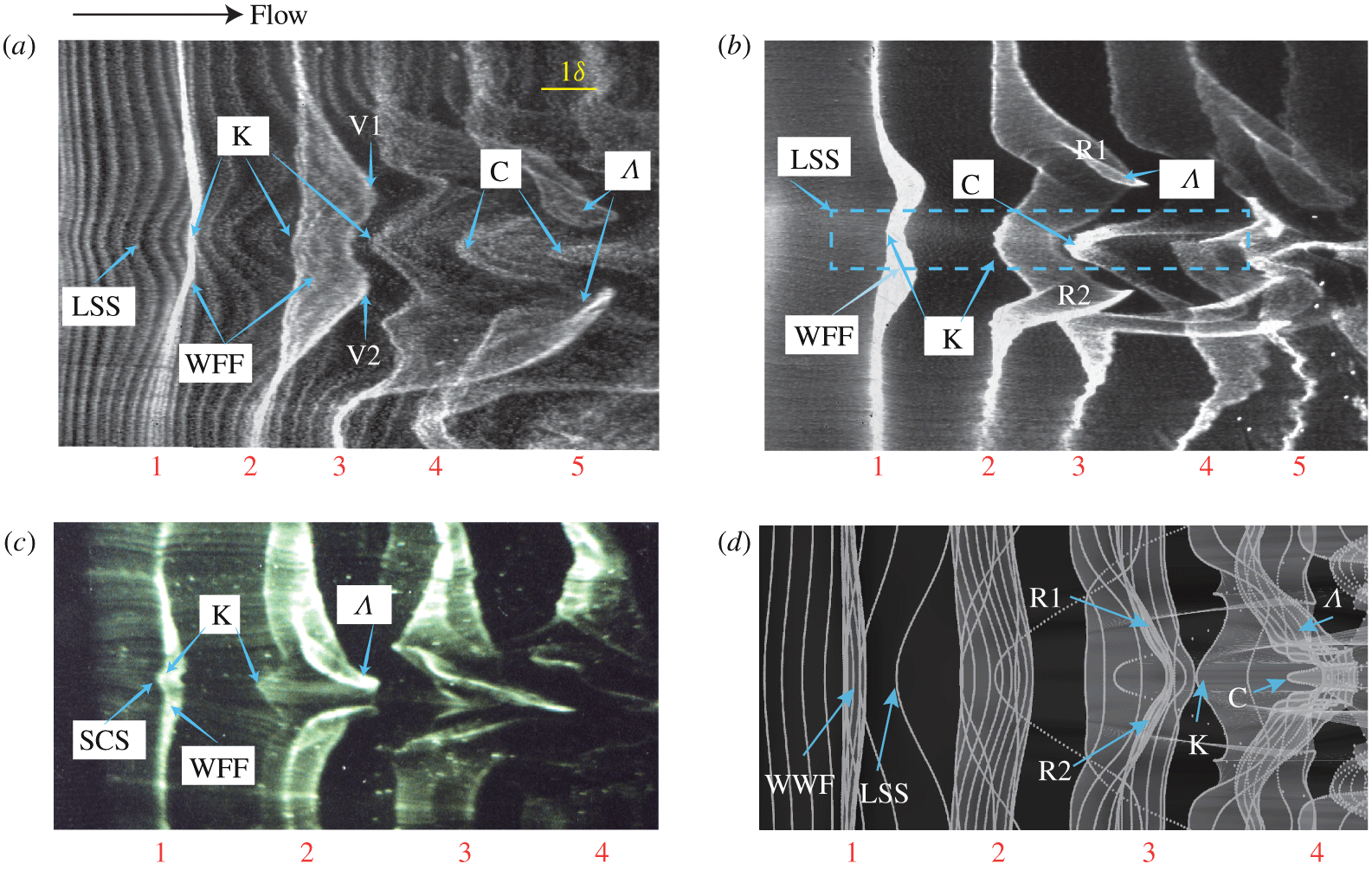
Figure 18(a,b) shows plan-view hydrogen bubble patterns in a controlled transitional boundary layer. The timelines in figure 18(a) clearly indicate a low-speed streak type of pattern, and also a downstream 𝛬-vortex straddling the streak. Note that there are several kink-like patterns that appear near the LSS, labelled as K in the figure. The 𝛬-vortex creates a butterfly-like pattern, which displays a ‘peak–valley’ behaviour. The two wings or ‘valleys’, labelled V1 and V2, pass over the timelines of the LSS and quickly surround the kink-like structure to form a 𝛬-vortex (see the supplementary Movie 8 for the complete evolution). Figure 18(b) also shows the same behaviour for a sheet of continuously generated hydrogen bubbles. The bubble sheet initially represents a warped wave front, stage 1 in the figure. The 𝛬-vortex is clearly seen to develop from the three-dimensionalized WWF (stage 2 in the figure). Progressing downstream, the kink-like patterns evolves into a much narrower chevron-like patterns (labelled C in the figure). Collectively, the patterns shown for the sequential stages in figure 18(b) are all associated with the formation of a LSS (within the dashed box). As shown by figure 18(a,b), the LSS appears to consist of several kink-like (or chevron-like) structures, encompassed by the 𝛬-vortex downstream. These patterns are markedly similar to hydrogen bubble visualizations by Lee (Lee Reference Lee2000; Lee & Fu Reference Lee and Fu2001; Lee & Li Reference Lee and Li2007; Lee & Wu Reference Lee and Wu2008), Hama & Nutant (Reference Hama and Nutant1963) and Wortmann (Reference Wortmann and Krause1981), an example of which is shown in figure 18(c). Combined with hot-film measurements within the kink-like region at different wall-normal heights, Lee et al. hypothesized that the kink-like pattern is a three-dimensional wave structure, termed a soliton-like coherent structure (SCS). The SCS was hypothesized as a natural consequence of the nonlinear amplification of a pair of oblique disturbance waves in the transitional boundary layer. Figure 18(d) is a timeline pattern from our NPSE study of K-regime transition, similar to figure 3, but with closer timeline spacing to more closely emulate to the hydrogen bubble visualization of figure 18(a). The brighter regions indicate where the timelines comprising the sheet are overlapping due to the folding process. This pattern looks markedly similar to the structures shown in figure 18(a–c), especially the patterns of the kink/chevron-like structures and 𝛬-vortex. The implications of these comparisons, and a hypothesis of the process that results in the development of the WWF and the 𝛬-vortex, will be discussed later in § 5.
Hydrogen bubble visualization of transitional boundary layer: (a) plan-view timelines at  $y=0.35\unicode[STIX]{x1D6FF}$; (b) continuous bubble visualization at
 $y=0.35\unicode[STIX]{x1D6FF}$ (c) low-speed streak and 𝛬-vortex at
 $y=0.15\unicode[STIX]{x1D6FF}$ (Lee & Wu Reference Lee and Wu2008); (d) ‘NPSE visualization’ of timelines initiated at
 $y_{0}=1.71$ for K-regime transition. The flow is left to right.

4.3 Comparison with ‘tomo-PIV visualization’
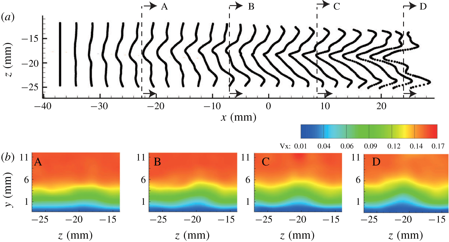
Low-speed streak development in a controlled transitional boundary layer at  $t=0.24~\text{s}$ after initiation. (a) Timelines generated from tomo-PIV;
 $x=0$ is a relative coordinate representing
 $X=378.5~\text{mm}$, with A, B, C, D indicating the streamwise location of the four cross-sections shown in 19(b); (b) cross-sections of streamwise velocity contours at: A,
 $x=-22.5~\text{mm}$; B,
 $x=-7~\text{mm}$; C,
 $x=8~\text{mm}$; and D,
 $x=24~\text{mm}$.

For the injection–suction controlled transition, the position of the low-speed streak is nearly stable, as shown in figure 19. Figure 19(a) is a plan view timeline visualization of a low-speed streak; figure 19(b) shows end-view cross-sections of streamwise velocity contours for the lifted low-speed streak. Figure 19(b) shows  $U$ contours at a sequence of four different streamwise locations in the
 $z$–
 $y$ plane (
 $x=-22.5~\text{mm}$,
 $-7~\text{mm}$, 8.5 mm, 24 mm) that illustrate the streamwise development of the LSS. As shown by the modest ‘hump’ region in these
 $U$ contours in plane A, the low-speed streak is initially very weak near the wall. As the streak develops downstream (planes B
 $\rightarrow$ C
 $\rightarrow$ D), the low velocity region expands in both the normal and spanwise directions, moving progressively upward. The presence and expansion of the low-velocity region is also apparent in figure 19(a), as revealed by the continued retardation of the simulated timelines. Note that these patterns of streak development are consistent with the behaviour of timeline patterns shown in end view in figure 5.
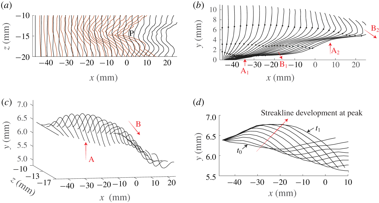
Figure 20 shows the spatial and temporal evolution of a LSS in a controlled transitional boundary layer. Figure 20(a) is superposed timeline patterns for timelines initiated at two different wall-normal heights. These patterns clearly show that the low-speed region (the peak region labelled P in the figure) is more pronounced near the bounding wall ( $y=0.4\unicode[STIX]{x1D6FF}$, red timelines), with significantly less retardation when the distance from the wall is doubled (
 $y=0.8\unicode[STIX]{x1D6FF}$, black time lines).
Spatial-temporal evolution of a low-speed streak reconstructed from the tomo-PIV data of a controlled transitional boundary layer: (a) plan view of superposed spanwise timelines at  $y=0.4\unicode[STIX]{x1D6FF}$ (red line) and
 $y=0.8\unicode[STIX]{x1D6FF}$ (black solid line); (b) vertical timelines released at
 $z=-13.7~\text{mm}$; markers indicate particles released at
 $y=0.2\unicode[STIX]{x1D6FF}$,
 $y=0.4\unicode[STIX]{x1D6FF}$,
 $y=0.8\unicode[STIX]{x1D6FF}$; A and B respectively indicate locations of lift-up and downward sweep events; (c) oblique view of the spanwise timeline pattern for timelines released at
 $y=0.8\unicode[STIX]{x1D6FF}$; (d) temporal evolution (
 $t_{0}\rightarrow t_{1}$) of streaklines initiated at a wall-normal position of
 $y=0.8\unicode[STIX]{x1D6FF}$, with time period
 $t=0.08T$ between realizations.

Figure 20(b) is a sequence of vertical timelines generated at a frequency of 10 Hz, and initiated at  $x=-45.8~\text{mm}$,
 $z=-13.7~\text{mm}$. Three streaklines are also shown in the figure, which initiate at
 $y=0.2\unicode[STIX]{x1D6FF}$,
 $y=0.4\unicode[STIX]{x1D6FF}$ and
 $y=0.8\unicode[STIX]{x1D6FF}$. The arrows labelled A and B in the figure indicate local organized vertical movements of the fluid. The two events labelled
 $\text{A}_{1}$ and
 $\text{A}_{2}$ are outward-directed lift-up events, and the two events labelled
 $\text{B}_{1}$ and
 $\text{B}_{2}$ are inward-directed sweep events. The inflectional region of the timelines is similar to the vertical hydrogen bubble visualization of a transitional boundary layer by Hama & Nutant (Reference Hama and Nutant1963). They considered the strong inflection to have its origin in a strongly ‘warped wave front’. Haidari & Smith (Reference Haidari and Smith1994) also observed this type of inflectional behaviour in a laminar boundary layer disturbed by injection through a streamwise slot. The ejection simulated a lift up of near-wall fluid, which was balanced by a downward sweep of outer fluid. The result was the creation of a high-shear layer between the ejection and the sweep, which was subsequently observed to break down into a hairpin vortex. These vertical timeline patterns, with the associated lift-up and downward sweep events are markedly similar to the K-regime simulation patterns shown previously in figure 6.
Figure 20(c) is an oblique view of the black timelines of figure 20(a), initiated at  $y=0.8\unicode[STIX]{x1D6FF}$. This figure clearly shows the development of a three-dimensional bulge, created by a preceding three-dimensional downward sweep (B), and a following three-dimensional lift up (A). Figure 20(d) shows the temporal evolution of streaklines initiated at
 $y=0.8\unicode[STIX]{x1D6FF}$ and
 $z=-13.7~\text{mm}$, the general location for the development of the peak position P in figure 20(a). It reveals a wave-like amplification of the streaklines in the upper boundary layer. Figure 20(c,d) suggests that the development of a ‘peak’ (LSS) propagates and amplifies as a wave-like structure.
Evolution of material surfaces reconstructed from the tomo-PIV data. The two surfaces are initiated at  $y=0.46\unicode[STIX]{x1D6FF}$ and
 $0.61\unicode[STIX]{x1D6FF}$ (initial flat surfaces shown at far right): (a)
 $t=0.16T$; (b)
 $t=0.32T$; (c)
 $t=0.48T$; (d)
 $t=0.64T$.

As pointed out in § 2.3, if the initial condition for Lagrangian tracking is a planar surface, the subsequent Lagrangian behaviour is that of an evolving material surface. Figure 21 shows the evolution of such a material surface for the present transitional boundary layer. The inset at the lower right of figure 21 shows two planar  $z$–
 $x$ material surfaces initiated at
 $y=0.46\unicode[STIX]{x1D6FF}$ and
 $0.61\unicode[STIX]{x1D6FF}$ (initially flat surfaces shown at the far right of figure 21). As these surfaces evolve in time, figure 21(a–d), they undergo a transverse warping, developing a peak/valley behaviour commented on previously that is construed as the development of a streamwise fluid lift up, flanked by apparent fluid sweeps toward the surface. The lower surface in figure 21(b), obtained at
 $t=0.32T$, illustrates the initial transverse warping of the material surface, with a peak (labelled P) developing at
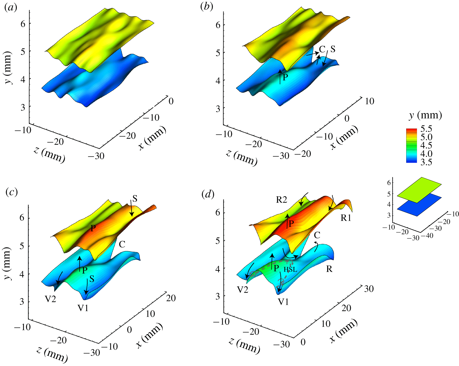
 $z\approx -20~\text{mm}$, the region where a LSS is observed. Downstream of the peak P, the material surface moves toward the centre, and develops a chevron-like pattern (labelled C). By
 $t=0.48T$, figure 21(c), the hump-like peak P is flanked by two material valleys, V1 and V2, due to the downward sweep motions. By
 $t=0.64T$, figure 21(d), a pronounced peak, P, has developed for both surfaces, which reflects the outward penetration of the LSS. The ejection/sweep motions create an HSL around the hump-like peak (dashed line in the figure), where an initial roll-up develops. The two distinct material valleys, V1 and V2, begin to subsequently roll up to form the legs of a 𝛬-vortex. The chevron-like pattern looks markedly similar to the hydrogen bubble visualization in figure 18(a), suggesting that a LSS is located beneath the humplike peak region. Note that the upper material surface does not appear as warped as the lower surface, i.e. the hump-like peak and the chevron-like pattern are more distinct on the lower surface, indicating that the HSL is also more pronounced at lower levels.
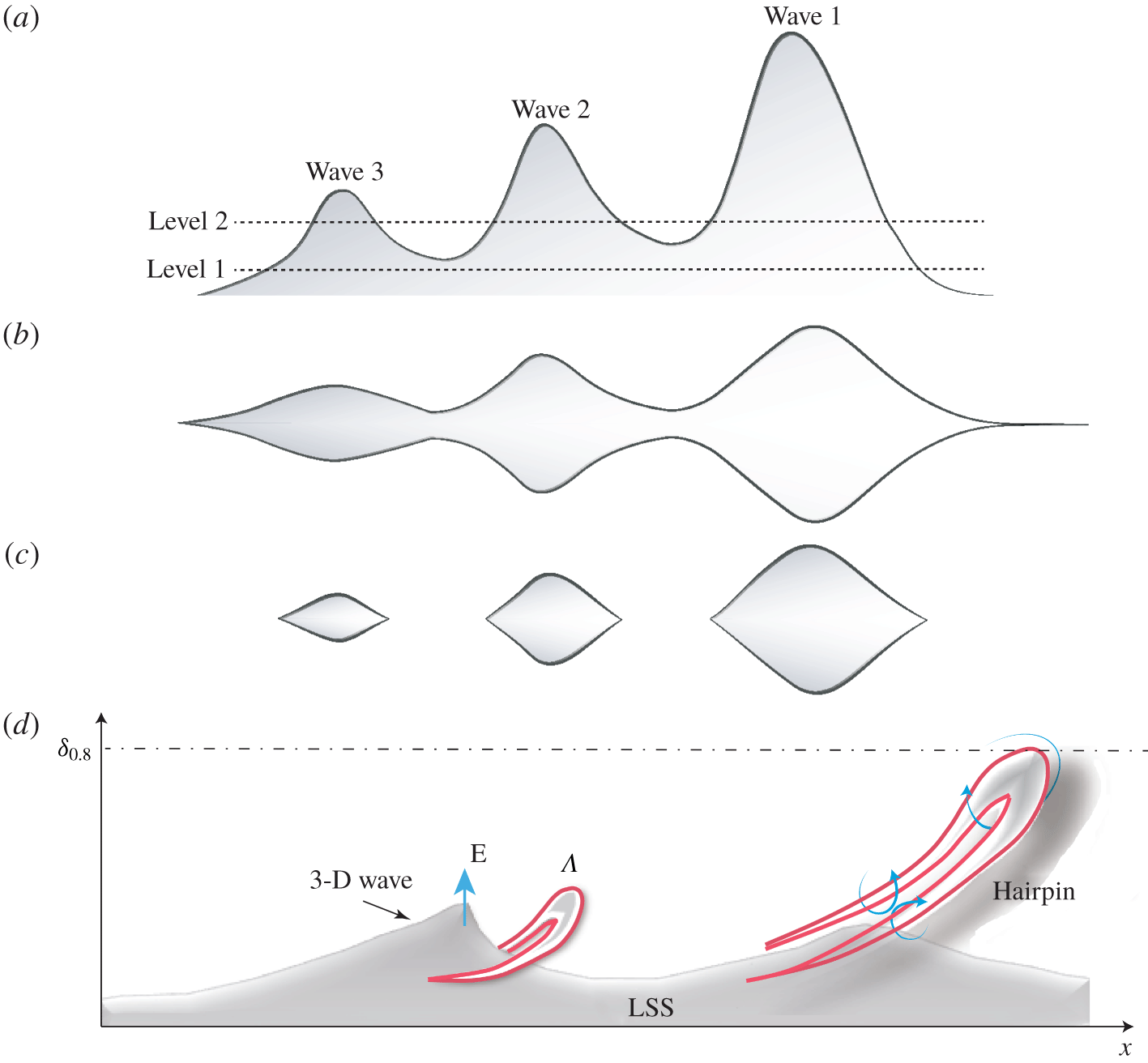
The evolutions of the material surfaces shown in figure 21 are supplements for the timeline patterns in figures 18 and 20. The bubble sheets appear much more convoluted than the material surfaces. But the evolution of the material surfaces caused by the developing flow field provides a more complete picture of the flow behaviour than the timelines. Both the evolution of the material surfaces (figure 21) and that of the hydrogen bubble sheet (figure 18) show that the LSS is flanked by developing vortices. And the LSS in figure 21 appears to lift up as a 3-D wave, the waveform of which is similar to that shown in figures 15(a) and 20(c,d). This suggests that the LSS revealed by the hydrogen bubble timelines of figure 18 is a 3-D wave structure, with the formation of vortices initiated by the lift up and breakdown of this 3-D wave.
5 Discussion
The linear stage of boundary-layer transition is relatively well understood, based on numerous experimental and linear stability studies. As the disturbances reach a finite amplitude where nonlinear effects become important, the flow becomes much more complicated because of nonlinear interaction between modes leading to energy exchange, and the development of new stages of three-dimensional instability. These subsequent stages are accompanied by different flow structures and motions whose cause and effect are difficult to resolve. The most common structures include 3-D waves, low-speed streaks, streamwise vortices, 𝛬-vortices (hairpin and ring-like vortices, and hairpin packets), which are usually associated with other fluid motions such as lift-ups, downward sweeps, roll-ups and entrainment, etc. In previous studies, there is no consensus on what causes the inflectional region and the low-speed streak formation. Additionally, details of how a warped wave front develops into a 𝛬-vortex is not well understood (Hama & Nutant Reference Hama and Nutant1963; Lee & Wu Reference Lee and Wu2008). The present study investigated the transitional boundary layer using a combination of selectively visualized NPSE and tomo-PIV data. The Lagrangian results of the present study allow these questions to be addressed, as well as revealing variations in the flow structure behaviour between different transition regimes. All these findings reveal the importance of three-dimensional waves in boundary layer transition.
5.1 Warped wave front
The results of the experiments and simulations show that the structures in the near-wall region sustain a higher shear than the upper region, with the material patterns near the wall revealing the development of an inclined and warped wave front. The concept of warped wave front was first proposed by Hama & Nutant (Reference Hama and Nutant1963) to describe the process of three-dimensional wave deformation prior to the formation of a discrete vortex. The WWF is observed to lift upward and amplify, with the front often stretched into thin filaments. This is clearly shown by the streakline patterns of figures 7, 13 and 14. The WWF in the near-wall region is observed to roll up as it propagates downstream. This roll up is observed as a folding behaviour of material surfaces, as shown in figures 3 and 8 and also in previous studies (Hama & Nutant Reference Hama and Nutant1963; Wortmann Reference Wortmann and Krause1981; Lee & Li Reference Lee and Li2007). The roll-up behaviour indicates the development of a vorticity concentration along the border of the wave front, which progressively develops into a discrete vortex. The processes of lift-up, amplification and roll-up usually cause the formation of inflectional points and three-dimensional high-shear layers.
The WWF is less warped in the upper region of the transitional boundary layer. As shown by figure 15 (and also the supplementary movies of Movie 2, Movie 4, Movie 6), all three transition regimes (K, O and N) display the same phenomenon of a lifted and amplified three-dimensional wave front accompanied by nearby regions of depression. The depression of the surface is considered to be caused by a downward sweep event compensating for the lifting low-speed fluid. Thus, it appears that the whole boundary layer during early-stage transition is dominated by amplified 3-D waves, which appear as strongly warped wave fronts in the near-wall region and less warped (or soliton-like) wave front in the upper region. The WWF is a three-dimensional wave packet, with convection speeds, determined by tracking the wave front, of 0.4– $0.45U_{\infty }$ during the early transition stage for all the three regimes.
5.2 Relation between 3-D wave structure and  $\unicode[STIX]{x1D6EC}$-vortex

The roll-up of streaklines, timelines or material surfaces can be easily misinterpreted as a vortex behaviour. Hama (Reference Hama1962) pointed out that the roll-up of a streakline does not necessarily indicate the presence of discrete vortices. The present study determined that the 𝛬-vortex will not develop until the multiple folding of a material surface occurs. The multiple folding behaviour here means that the continuing amplification of a 3-D wave causes the lower portion of a warped wave front to lift up and progressively dominate the wave front. The ‘kernel’ studies for the three transition regimes show the details of how a 𝛬-vortex develops from a 3-D wave (figures 4, 5, 9, 10), which agrees with the observations of Klebanoff et al. (Reference Klebanoff, Tidstrom and Sargent1962) and Hama & Nutant (Reference Hama and Nutant1963), that three-dimensionality appears prior to an appreciable vorticity concentration along the swept-back sides of the wave front. What we found is that the multi-folding process caused by a lifting 3-D wave has a close relationship to the formation of a 𝛬-vortex. It implies that the 3-D wave plays an active role in vorticity concentration that results in the formation of a 𝛬-vortex.
Figure 22 provides a schematic model of the development of 3-D wave behaviour, and its subsequent development into a 𝛬-vortex/hairpin vortex. As shown in figure 22(a), an initial 3-D wave is produced by interaction between different modes, depending on the particular transition regime. The amplification and lift-up of this 3-D wave disturbs the boundary layer, resulting in low-speed fluid being ejected from the near-wall region upward (ejection event labelled E in figure 22). This ejection process is responsible for the development of a kink structure in vertical timelines, such as the inflectional region that appears as a hump in figures 6, 11 and 12. As the low-speed fluid is ejected outward, higher-speed fluid passing above the 3-D wave sweeps downward (labelled S in figure 22) to compensate for the lifting low-speed fluid. This adjacent fluid inflow and outflow creates an inclined, localized 3-D high-shear layer (LHSL) at the interface of the 3-D wave during its lift-up, as indicated by the red lines in figure 22(a). A black dashed line, adjacent to the 3-D wave, models the development of the warped wave front, according to the streakline patterns of figures 7, 13 and 14. Note that the streakline is actually three-dimensional; what we show here is its projection on the  $x$–
 $y$ plane.
Schematic view of the development of a 3-D wave. (a) Initial 3-D wave causes the development of a warped wave front; (b) amplified 3-D wave induces the second folding; (c) 𝛬-vortex appears.  $\unicode[STIX]{x1D6FF}_{0.8}$ indicates the wall-normal position of
 $0.8U_{\infty }$; the black dashed line adjacent to the 3-D wave models the development of a streakline; the red line indicates the development from a high-shear layer to a 𝛬-vortex. E, ejection event.

Figure 22(b) shows that as the 3-D wave amplifies, it extends rapidly upward, causing the high-shear layer to strengthen, a concentration of vorticity to develop, followed by an initial vortical roll-up of the HSL (red lines). The streakline in figure 22(b) reflects a second folding behaviour, with a lower portion of the warped wave front projecting upward above the leading edge of the wave. In the timeline visualization of figure 4, the initial vortical roll-up develops along the swept-back portion of the wave front, which is the initial appearance of a 𝛬-vortex. As the 3-D wave advects downstream, figure 22(c), it continues to grow outward, eventually extending above the critical layer, where it loses symmetry and begins to breakdown to a 𝛬-vortex. As figure 22(c) shows, a 𝛬-vortex subsequently forms from the HSL with its head inclined upward, similar to the ring-like vortex model suggested by previous studies (Lee & Fu Reference Lee and Fu2001; Guo et al. Reference Guo, Borodulin, Kachanov, Pan, Wang, Lian and Wang2010). The second folding of the streakline will progressively become a second warped wave front. The location of this second folding was found to form the head of a 𝛬-vortex. Note that this second folding behaviour was not observed in the simulation of a shear flow perturbed by one or two non-amplifying travelling waves (Hama Reference Hama1962; Williams & Hama Reference Williams and Hama1980). This further supports the importance of the amplified 3-D wave in the formation of a 𝛬-vortex.
Figure 22(c) also models a lower portion of the streakline as deforming strongly to yield a sharp ridge (filament, labelled D), which moves upward and rearward, modelled after the streakline behaviour shown in figure 14. This ridge formation is due to a combined lift-up of fluid by the amplified 3-D wave and a retardation caused by the developing counter-rotating legs of the 𝛬-vortex.
5.3 Low-speed streaks in transition
Schematic views of a transitional low-speed streak: (a) schematic side view of a hypothesized low-speed streak model, comprised of three contiguous SCSs; (b) schematic plan view of the LSS model at height level 1; (c) schematic view of plan view of the model at height level 2. (d) Relation between 3-D wave, low-speed streak and vortices.

The present study determined that the LSS is correlated with the development of kinked patterns in vertical timeline sheets (labelled K in figure 6), chevron-like patterns in transverse timeline sheets and material surfaces (labelled C in figures 4, 9, 10, 18, 21). The LSS is also reflected by the retarded streaklines (labelled D in figures 14 and 22). As discussed in § 5.2, the behaviour of those time-material visualizations is closely related to the amplification of a 3-D wave, and the low-speed streak appears to collectively consist of several wave structures. A schematic concept of the LSS structure is represented schematically in figure 23(a–c). The wave model assumes that three waves align in the streamwise direction. These 3-D waves would appear to propagate from left to right, while moving away from the wall, as suggested by Movies 1–4 and also the hydrogen bubble visualization in the very near-wall region of a transitional boundary layer (Lee & Wu Reference Lee and Wu2008). The schematic model in figure 23(a–c) shows hypothesized side-view and plan-view models of a low-speed streak consisting of three contiguous wave structures. Near the wall (i.e. level 1 shown in figure 23a), the three waves combine to form an interconnected domain, which could be interpreted as a continuous structure, as shown in figure 23(b). However, further removed from the wall (i.e. level 2 in figure 23a), isolated wave patterns, such as shown in figures 23(c), would appear as separate structures. These isolated wave structures are like those visualized in figures 15.
Figure 23(d) provides a conceptual model showing the relation between 3-D waves, low-speed streaks and vortices. As mentioned previously, a low-speed streak develops beneath a passing 3-D wave, which suggests that amplification of the 3-D wave produces the LSS pattern at early-stage transition. However, as the attached 𝛬-vortex finally develops into a discrete hairpin vortex, it will in turn induce a low-momentum region at the centre of its legs. Thus, streaky structures in late-stage transition or within a turbulent boundary layer are longer and narrower, characterized by oscillation and undulation (Kline et al. Reference Kline, Reynolds, Schraub and Runstadler1967; Sandham & Kleiser Reference Sandham and Kleiser1992; Adrian, Meinhart & Tomkins Reference Adrian, Meinhart and Tomkins2000). Therefore, the LSSs in less organized boundary layers (late transition/turbulent) are possibly the result of a combined interaction between 3-D waves and hairpin vortices (or packets), which needs to be further investigated. Note that the model shown in figures 22 and 23 is similar to the model of hairpin vortex generation by the break-up of a synthetic LSS shown in Acarlar & Smith (Reference Acarlar and Smith1987b). It was hypothesized by Smith (Reference Smith, Patterson and Zakin1984) that the passage of a vorticity concentration created upstream can create a transient, spatially varying pressure gradient which could precipitate the local deceleration and three-dimensional oscillation. Instead, the current discussion attributes the cause of the oscillation and vorticity concentration to the amplification and lift-up of a 3-D wave.
The differences and similarities between the various transition regimes have been discussed in a number of studies (Zhou & Liu Reference Zhou, Liu, Meier and Bradshaw1987; Boiko et al. Reference Boiko, Westin, Klingmann, Kozlov and Alfredsson1994; Elofsson Reference Elofsson1998; Berlin et al. Reference Berlin, Wiegel and Henningson1999; Bake et al. Reference Bake, Fernholz and Kachanov2000; Lee Reference Lee2000; Schmid & Henningson Reference Schmid and Henningson2001), most of which focused on late-stage transition. The results of the present study indicate that a universal transition mechanism may exist, and can account for the similarities and differences of the three regimes. The possible common route may rely on the amplified warped wave front. All the three regimes share oblique modes, the interaction of which results in WWF and streaks. Near the wall within a laminar boundary layer, the lift-up of a WWF amplifies the already higher-shear layer, creating in a strong localized 3-D high-shear layer, which subsequently forms the initial 𝛬-vortex. Later, the development of the 𝛬-vortex and its variants complicate the near-wall fluid behaviour, which will further contribute to the ejection–sweep cycle (or bursting process). The WWF discussed in this study is similar to ‘soliton-like coherent structure’ (Lee & Chen Reference Lee, Chen, Ged-el Hak and Tsai2006), especially in the outer region of the boundary layer.
6 Conclusions
In this study, solutions to a nonlinear parabolized stability equation and the results of complementary experiments are used to investigate the early-stage process of boundary-layer transition. Three kinds of transition regimes were considered, i.e. K-regime, N-regime and O-regime. However, only the K-regime transition was examined experimentally using both hydrogen bubble visualization and time-resolved tomographic particle image velocimetry (tomo-PIV).
A structure-based view was provided in this paper, combined with analysis of mode evolution. Using Fourier decomposition, it was determined that small oblique disturbances are strongly amplified by resonance with the larger fundamental disturbances for the K- and N-regime, and that zero-frequency modes grow fast due to the interaction of oblique modes for the O-regime. Lagrangian particle tracking was applied on the NPSE and tomo-PIV database to extract the evolution of structures. According to the numerical and experimental visualizations, at least four common characteristics of the generic transition process were identified: (i) an inflectional region appears in vertical streamwise velocity profiles, accompanied by ejection–sweep behaviours; (ii) horizontal timelines display a chevron-like structure in the near-wall region, which subsequently develops into a long, narrowed streaky structure (LSS); (iii) a warped wave front displaying multiple folding behaviour and wave-like amplification/damping behaviour, which develops adjacent to the LSS in the near-wall region, prior to the appearance of 𝛬-vortices; (iv) development of a coherent 3-D wave front similar to a soliton within the upper boundary layer, accompanied by regions of depression along the flanks of the wave. The results revealed that an amplified WWF comprising the LSS causes multiple folding behaviour, leading to a 𝛬-vortex in the near-wall region.
Based on the similarities between the different transition regimes, the following hypothesis for general transition is proposed. The transition is initiated by the growth of 2-D T–S wave and oblique waves (only oblique waves for O-regime transition), with zero-frequency modes growing progressively at later stages further downstream. The nonlinear interaction of oblique waves seems to be the core of the wave resonance, which contributes to an amplified 3-D wave appearing as a WWF. During the wave amplification process, a LSS develops near the wall, which is composed of several WWFs. A subsequent lift-up of a WWF disturbs the boundary layer by ejecting low-speed fluid upward from the near-wall region, resulting in the development of kink structures in both vertical and horizontal velocity profiles. Due to mass conservation, higher-speed fluid in the outer region sweeps downward, creating a forward inclined, localized 3-D high-shear layer (LHSL) at the edge of the 3-D wave. The amplification of the WWF further strengthens the LHSL, leading to a concentration of vorticity within the LHSL that initiates a vortical roll-up process. This vortical roll-up of the LHSL creates a 𝛬-vortex, which subsequently separates from the wave front as a distinct flow structure. The counter rotating legs of the 𝛬-vortex (or hairpin vortex) help concentrate low-momentum fluids on its plane of symmetry, reinforcing the LSS and the WWF. However, the upper portion of the WWF is longer lived, propagating downstream like a soliton, which indicates that the WWF is the same structure as soliton-like coherent structure (SCS).
The model proposed above is based primarily on our assessment of the reconstructed timeline and surface visualization patterns, which are not without approximation, and are of course open to the bias of the viewer. However, our assessment of the patterns, and the synthesis of these assessments into a model of the generic transition process, provides a rational, structural description of how early-stage transition develops. Clearly, more study is necessary to confirm the model, but it is clearly a reasonable starting point. The model also provides a platform to move on to the assessment of the more irksome counterpart to transition – the process for sustaining turbulent behaviour in a boundary layer.
Acknowledgements
This work was supported by the National Natural Science Foundation of China (10921202, 11221061, 11632002, 11521091 and 11602005) and National Key Project GJXM92579.
Declaration of interests
The authors report no conflict of interest.
Supplementary movies
Supplementary movies are available at https://doi.org/10.1017/jfm.2020.107.