Vegetal species’ non-communicative art

The life story I will first discuss looks at the displacement of vegetal species across southern and northern hemispheres. Prehistoric peoples across the neotropics engaged in plant cultivation and transportation outside their area of origin in South America, with recent research suggesting that plant cultivation may have preceded plant domestication, and that maize is a case of successful adaptation to a range of environmental circumstances before its domestication (Piperno Reference Piperno2011: 463–464). Later, at the end of the ninetieth century, pine afforestation in the southern hemisphere, starting in South Africa and followed by New Zealand and Australia, developed forestry industries as a main colonial economic activity (Burgess and Wingfield Reference Burgess and Wingfield2001). European settlements in the southern hemisphere also increased farming on slopes which reduced plant cover causing large landslides, which in turn triggered further displacements of civilisations carrying seeds with them (Leroy Reference Leroy2022). These stories of vegetal species displacement and geological erosion are told through the embedment of algorithms in my work Landslide (2023), which seeks to examine the non-communicative vegetal art that Le Guin (Reference Le Guin, Silverberg and Greenberg1988) envisages in The Author of the Acacia Seeds.

Le Guin (Reference Le Guin, Silverberg and Greenberg1988) describes a fictional future in which therolinguists fail to decipher the art of plants because their approach is based on animals’ kinetic literature when plant art is non-kinetic. The story ends with an excursion of phytolinguists who decipher plant lyrics only to be outpaced by the first geolinguist to read the ‘wholly atemporal, cold, volcanic poetry of the rocks’ (Le Guin Reference Le Guin, Silverberg and Greenberg1988: 518). This story leads me to ask: What form may plant art take? How does it sound? How does the volcanic poetry of the rock sound? Haraway’s (Reference Haraway2016: 122–124) response to The Author of the Acacia Seeds provides insights into plants’ communicational means, understood not as a linguistic one but rather as actions that bound ants and plants in exchanges that sustain the lives of either species. I thus sought to enquire the sonic textures of plants and rocks through actions that create concrete relations with specific vegetal and mineral matter.

Landslide explores sound-making gestures performed with corn grains, pine cones and needles, and rocks on percussion instruments. The sounds produced are captured by contact microphones placed on each instrument’s surface and processed in real time. The percussion instruments are placed horizontally so that they contain the grains, pine cones and rocks on top of them. A camera captures an overhead view of the instruments (whose live feed is projected during the live performance), which centres the narrative on the vegetal and mineral materials and on the hands of the performers only, as shown in Figure 1.

Figure 1.

Landslide studio recording.

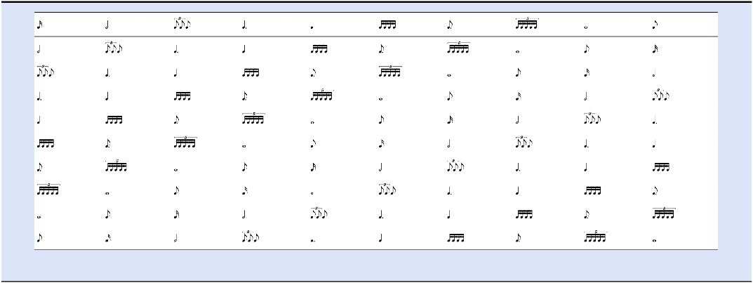
I found making sound through and with the specific materiality of vegetal species to be a more appropriate approach to telling their stories than attempting to decipher their language. To organise the narrative structure of the piece, I encompassed the facts in the maize, pines’ and rocks’ stories into seven sequential phases: 1) each species is on a separate instrument (geographic location), with rhythms and gestures performed individually without affecting each other’s actions; 2) the performers placed on the outer sides play on the tam-tam placed in the middle, expanding their areas of influence, and the corn grains are grouped in portions as in human selection of wild variants; 3) corn grains are displaced to the centrally located drum which modifies the rocks’ arrangement, while pine scales and needles are grouped into portions which illustrates the quarantine methods applied to conifers when imported to South Africa and Australia (Burgess and Wingfield Reference Burgess and Wingfield2001); 4) pine scales and needles are displaced to the centrally located drum which further modifies the rocks’ arrangement, while the disposition of the corn grains remaining on the gran cassa is modified; 5) each performer mixes the materials now placed on each drum; 6) the performers play fast and loud rhythms on each drum that further disrupt the disposition of the materials and 7) in turn, each performer grabs the materials on their instrument, drops them on other instrument’s surface, then leaves. To generate rhythmic material that would bear a formal relationship with this narrative structure and that I could develop through algorithmic permutations, I created a progressive series composed of seven rhythmic cells. The first cell consists of a single rhythmic figure followed by a cell that articulates two time values, successively adding one rhythmic value (in terms of articulation and not of total duration) so that the last cell articulates seven notes, which is shown in Table 1.

Table 1.

Rhythmic cells series

Table 1. Long description

A musical notation displaying a sequence of rhythmic cells. The notation is divided into seven distinct phases, each representing a different rhythmic pattern. The first cell features a single rhythmic figure, followed by cells that progressively add one rhythmic value in terms of articulation, culminating in a cell that articulates seven notes. Each phase is visually represented by musical notes and rests, indicating the timing and duration of each rhythmic element.

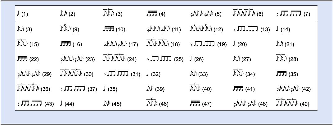
Winterson (Reference Winterson2024) analyses the use of magic squares to generate musical material in serial works by Peter Maxwell Davies, Pierre Boulez and Phillipe Manoury as well as the use of Latin squares in serial works by Anton Webern and Bruno Maderna. I used both square types to generate combinations of the rhythmic cells in the series. I first permutated the cells in the row in the seven ways possible and arranged them in a Latin square, that is, a square array in which each row or column contains each cell precisely once as shown in Table 2. This created a Latin square of order 7 with a total of 49 cells. The rotations of the series presented in the rows below the top row in the square are calculated through the following algorithm.

$$\matrix{ {If \,L\,\left( {i,j} \right){\rm{ is\, the\, entry\, in\, row }}\,i,{\rm{ column }}\,j,{\rm{ where }}\,i,j \in \left\{ {0,{\rm{ }} \ldots, {\rm{ }}6} \right\},} \cr {{\rm{and }}\,S\,\left\{ {s0,{\rm{ }} \ldots, s6} \right\}{\rm{\, is\, the\, ordered\, series\, in\, the\, first\, row,\, then}}} \cr {L\,\left( {i,j} \right){\rm{ }} = S\,\left( {i + j} \right)\,{\rm{ mod }}\,7} \cr }$$

Table 2.

Latin square permutations, numbered 1–49

Table 2. Long description

An equation describing the algorithm for generating Latin square permutations. The equation defines the entry in row i, column j of a Latin square, where i and j range from 0 to 6. The entry L(i,j) is determined by the ordered series S in the first row, using the formula L(i,j) equals S(i plus j) mod 7.

Each row contains the first row shifted left by i places. Upon reaching the seventh cell, ‘mod 7’ at the end of the calculation continues the sequence again from the first cell of the series. The 9 rotations obtained are shown in Table 2.

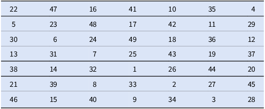
I also employed the 7 × 7 magic square shown in Table 3, a square matrix in which each horizontal, vertical and diagonal row of 7 different integers adds up to the number 175.

Table 3.

7 × 7 magic square matrix

Table 3. Long description

A table representing a 7x7 magic square matrix. The table has 7 rows and 7 columns, each containing unique integers. The numbers in each row, column, and diagonal add up to 175. Row 1: 22, 47, 16, 41, 10, 35, 4. Row 2: 5, 23, 48, 17, 42, 11, 29. Row 3: 30, 6, 24, 49, 18, 36, 12. Row 4: 13, 31, 7, 25, 43, 19, 37. Row 5: 38, 14, 32, 1, 26, 44, 20. Row 6: 21, 39, 8, 33, 2, 27, 45. Row 7: 46, 15, 40, 9, 34, 3, 28.

This magic square is constructed using the following algorithm:

The rows and columns are also indexed: i, j ∈ {0, 1, 2, 3, 4, 5, 6}.

Then two auxiliary values are computed as follows.

$$U\left( {i,{\rm{ }}j} \right){\rm{ }} = {\rm{ }}\left( {4i + {\rm{ }}3j + {\rm{ }}3} \right)\,{\rm{ mod\, 7}}$$

$$V\left( {i,{\rm{ }}j} \right){\rm{ }} = {\rm{ }}\left( {4i + {\rm{ }}4j} \right)\,{\rm{ mod\, 7}}$$

Finally, the two auxiliary values are combined to calculate the entry of the square.

$$M\left( {i,{\rm{ }}j} \right){\rm{ }} = {\rm{ }}7U\left( {i,{\rm{ }}j} \right){\rm{ }} + V\left( {i,{\rm{ }}j} \right){\rm{ }} + {\rm{ }}1$$

For example, to calculate the entry in row i = 1, column j = 6 the procedure below applies.

$$U\left( {1,\;6} \right)\; = \;(4 \cdot 1\; + \;3 \cdot 6\; + \;3)\,{\rm{ mod \,7 }} \,\,\,\,\,\,\,\,\,\,\,\,\,\,\,\,\,\,\,\,\,\,\,\,\,\,\,\,\,\,\,\,\,\,\,\,\,\,\,\,\,\,\,\,\,\,\,\,\,\,\,\,\,\,\,\,\,\\ = \;\left( {4\; + \;18\; + \;3} \right){\rm{ \,mod\, 7 }} = \;25{\rm{\, mod\, 7 }} = \;4$$

$$\eqalign{V\left( {1,\;6} \right)\; & = \;(4 \cdot 1\; + \;4 \cdot 6){\rm{ \,mod\, 7 }} = \;\left( {4\; + \;24} \right){\rm{ mod\, 7 }}\cr & = \;28{\rm{ \,mod\, 7 }} = \;0}$$

$$M\left( {1,\;6} \right)\; = \;7 \cdot 4\; + \;0\; + \;1\; = \;29$$

The algorithm that structures this magic square wraps numbers in 7 cycles of size 7 separated by +7 (such as 1 8 15 29 36 43, 2 9 16 23 30 37 44). These cycles are concatenated in the magic square (Table 3), creating patterns that descend diagonally across the matrix and continue in the first row and the following column upon reaching the bottom row. For example, the cycle 1–43 starts in (i4, j3), continues in (i5, j2), (i6, j1), (i0, j0), (i1, j6), (i2, j5) and finishes in (i3, j4). This pattern may be regarded as an illustration of the displacement of the plants across the hemispheres, moving towards the lower end of the square and continuing the trajectory with a leap to the upper region.

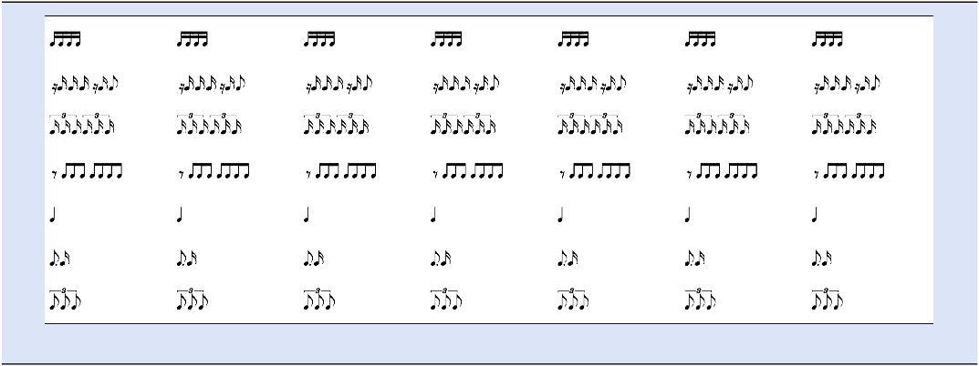
Upon numbering the cells in the initial Latin square starting from the furthermore left top cell (see Table 2), each column, which contains the cells once, was assigned one of the +7 modular cycles. I then mapped the cells onto the 7 × 7 magic square matrix, following the order in which the assigned numbers are distributed in the magic square, as shown in Table 4. As a result, the columns of the Latin square were arranged following the patterns of the modular cycles. Because each row intersects every cycle exactly once, and each cycle corresponds to a complete series featuring each rhythmic cell once, horizontal rows of seven equal rhythmic cells were obtained (Table 4).

Table 4.

Series permutations mapped onto the 7 × 7 magic square matrix

Table 4. Long description

Table showing seven repetitions of seven rhythmic patterns, arranged in seven columns and seven rows. Each column contains the same sequence of rhythmic figures. From top to bottom, these comprise a group of four semiquavers; a syncopated figure combining two semiquaver rests, four semiquavers and a quaver; two groups of semiquaver triplets; a quaver rest followed by seven quavers; a single crotchet; a dotted quaver followed by a semiquaver; and a quaver triplet. Each rhythmic pattern is repeated seven times across its respective row.

Subsequently, the material suggested by the 7 × 7 square matrix arrangement informed musical events notated in the score. In phase 1 (Figure 2), the fifth row was used in the first event written for the gran cassa and the seventh row in the first event written for the tam-tam. Further material was also developed taking different routes through the Latin square matrix. For instance, the third event in the gran cassa part (phase 1, Figure 2) originates from the furthest left cell of the fourth row ascending one cell diagonally, then one cell upwards and then one cell left. In phase 1, players are requested to perform the events within the boxes in any order. This creates iterative rhythmic tiling canons underpinned by the presence of repeated rhythmic cells in the different instrumental parts.

Figure 2.

Landslide score, phase 1.

In phase 2 (Figure 3), a retrograde movement of the sixth row of the magic square is played on the tam-tam by the gran cassa player. In the first system, the timpano plays a diminution of the first half of the seventh rhythmic cell of the initial series. Phase 2 also features graphics devised to notate gestures performed in specific interaction with the materials examined, such as the zig-zag motion that disrupts the line traced by the rocks and the arrangement of the corn grains in groups.

Figure 3.

Landslide score, phase 2.

The live electronics process sounds captured with contact microphones placed on the instruments’ resonating heads, which are produced through contact with the corn grains, pine cones and needles, and rocks. The real-time timbre transformation applied consist of filtering the frequencies and either lowering or raising the (undetermined) pitches captured (to view a studio recording, see Luciana Perc Reference Perc2024a in the Videography section below). While the algorithms computed in these sound treatments are not discussed in this section, the fourth section considers the algorithms applied in similar real-time sound processes in detail. The microphones, together with the applied digital processes, act as an aural magnifying glass that amplifies the sounds produced by human hands as well as by vegetal and mineral matter, drawing attention to the lives of plants and rocks that are unable to avoid human impact on them. The stories told in Landslide are stories of vegetal species displacement and soil erosion. The motivations of the human-led displacements of vegetal species addressed are both economic and social. In turn, the adaptative responses (in genetic evolutionary terms) of, and the diseases suffered by, plants had an impact on human subsistence and economic growth (Burgess and Wingfield Reference Burgess and Wingfield2001; Piperno Reference Piperno2011). Rather than proposing a quantitative understanding of such exchanges between vegetal and human species, the sonic reconfigurations described foreground the seven stages of a shared history of mutual transformations. By way of focusing on the sonic materiality of vegetal and mineral species, the piece engages with a new materialist understanding of natural-cultural practices that cuts across the well-worn divides that conceptualise materiality either as strictly economic or purely social (Barad Reference Barad2007: 226). Moreover, examining vegetal and mineral species through bodily sound production enables this reconfiguration process through hypermedial means (Havelková Reference Havelková2021).

Meeting the sound of the universe halfway

The final words in The Author of the Acacia Seeds captivated my imagination towards the idea that, through the assortment of its soil, the earth speaks to the greater community of space. In her search for an unheroic science fiction, Le Guin points us to the myths of creation as a way in which people have been telling life stories (Le Guin Reference Le Guin2019: 34). I therefore embedded a scientific simulation of the formation of a galaxy, specifically the ASURA simulation (Saitoh et al. Reference Saitoh, Daisaka, Kokubo, Makino, Okamoto and Tomisaka2008), into a musical composition through algorithms I designed using data from this simulation. The sonification of astronomical data has been explored with the aim of expanding the means of scientific observation (Diaz-Merced et al. Reference Diaz-Merced, Candey, Brickhouse, Schneps, Mannone, Brewster and Kolenberg2012). Conversely, a range of scientific dissemination projects that disseminate cosmological observations convert image data to sound (to view examples of such projects see NASA 2025). The latter’s aesthetic approach to the sonification of image data draws on tonal music narrative structures as used in science fiction film music, the science fiction stories that Le Guin’s depicts as the mythology of modern technology, embodied as triumphant myths of conquest. This section discusses a compositional study that challenges such aesthetic approach to the dissemination of astronomical data and its semantic implications through a reconfiguration approach to the use of cosmological data in an intermedial composition. Virtual Galaxy Simulation (2023/24) is a work for ensemble with octophonic electronics and video projection scored to the visualisation of the ASURA simulation of a galaxy formation and composed for the contemporary music ensemble Proxima Centauri. As shown in Figure 4, the visualisation of the galaxy formation simulation is projected above the musicians during the performance of the piece, who follow a click track to play in synchronisation with the video (See Luciana Perc Reference Perc2024c to view the video recording of the performance, which features a projection of the visualisation of the ASURA simulation).

Figure 4.

Performance of Virtual Galaxy Simulation. Ph credit: Frederic Desmesure.

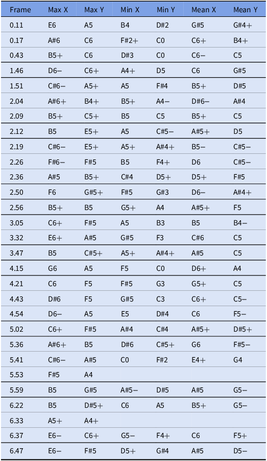
The compositional process examined how to organise astronomical data to create a score for instrumental ensemble. The working theory of spiral galaxy formation explains that sparse particles are attracted by the gravity of higher density masses, which causes smaller galaxies to rotate around greater ones until they finally merge. Gas reaches high temperatures during the spiral waves phase and galaxies achieve their definite structure when gas cools and rotation stops. The ASURA simulation of galaxy formation maps gas temperature and particle density to different colours and brightness grading (Saitoh et al. Reference Saitoh, Daisaka, Kokubo, Makino, Okamoto and Tomisaka2008: 672). These two temperature and density variables change throughout the simulation providing propitious circumstances for the formation of spiral galaxies. I developed a procedure to capture said changes in numerical data that could be translated into series of pitches. I started by selecting a total of 29 frames from specific time codes in the video where changes in the colour grading and the dispersion of particles in the image were significant (Figure 5 provided as an example). I deployed a spectral analysis of the selected frames with the astronomical analysis software AstroImageJ.

Figure 5.

Frame at time code 1.51.

The analysis outputs a list of bidimensional coordinates (corresponding to pixels grids used in AstroImageJ’s spectral analysis) of the points of maximum, medium and minimum brightness. I considered the values of the coordinates as if they were frequencies expressed in Hz and collected the pitches obtained for each time code into a list, shown in Table 5. I treated the coordinates values as frequencies in Hz, yet not every value would match the frequency of a specific note in the equal temperament system. The methodological approach I chose was to map each value to the closest note within a microtonal system. The symbol + indicates the note sounds a quarter tone higher and – a quarter tone lower.

Table 5.

Virtual Galaxy Simulation, pitches obtained for each frame’s coordinates

Table 5. Long description

A table comparing coordinates and pitches for each frame in a virtual galaxy simulation. The table has 30 rows and 7 columns. Column headers are Frame, Max X, Max Y, Min X, Min Y, Mean X, and Mean Y. Row 1: Frame, 0.11; Max X, E 6; Max Y, A 5; Min X, B 4; Min Y, D sharp 2; Mean X, G 5; Mean Y, G sharp 4 plus. Row 2: Frame, 0.17; Max X, A sharp 6; Max Y, C 6; Min X, F sharp 2 plus; Min Y, C 0; Mean X, C 6 plus; Mean Y, B 4 plus. Row 3: Frame, 0.43; Max X, B 5 plus; Max Y, C 6; Min X, D 3; Min Y, C 0; Mean X, C 6 minus; Mean Y, C 5. Row 4: Frame, 1.46; Max X, D 6 minus; Max Y, C 6 plus; Min X, A 4 plus; Min Y, D 5; Mean X, C 6; Mean Y, G 5. Row 5: Frame, 1.51; Max X, C sharp 6 minus; Max Y, A 5 plus; Min X, A 5; Min Y, F sharp 4; Mean X, B 5 plus; Mean Y, D 5. Row 6: Frame, 2.04; Max X, A sharp 6 plus; Max Y, B 4 plus; Min X, B 5 plus; Min Y, A 4 minus; Mean X, D sharp 6 minus; Mean Y, A sharp 4. Row 7: Frame, 2.09; Max X, B 5 plus; Max Y, C 5 plus; Min X, B 5; Min Y, C 5; Mean X, B 5 plus; Mean Y, C 5. Row 8: Frame, 2.12; Max X, B 5; Max Y, E 5 plus; Min X, A 5; Min Y, C sharp 5 minus; Mean X, A sharp 5 plus; Mean Y, D 5. Row 9: Frame, 2.19; Max X, C sharp 6 minus; Max Y, E 5 plus; Min X, A 5 plus; Min Y, A sharp 4 plus; Mean X, B 5 minus; Mean Y, C sharp 5 minus. Row 10: Frame, 2.26; Max X, F sharp 6 minus; Max Y, F sharp 5; Min X, B 5; Min Y, F 4 plus; Mean X, D 6; Mean Y, C sharp 5 minus. Row 11: Frame, 2.36; Max X, A sharp 5; Max Y, B 5 plus; Min X, C sharp 4; Min Y, D 5 plus; Mean X, D 5 plus; Mean Y, F sharp 5. Row 12: Frame, 2.50; Max X, F 6; Max Y, G sharp 5 plus; Min X, F sharp 5; Min Y, G 3; Mean X, D 6 minus; Mean Y, A sharp 4 plus. Row 13: Frame, 2.56; Max X, B 5 plus; Max Y, B 5; Min X, G 5 plus; Min Y, A 4; Mean X, A sharp 5 plus; Mean Y, F 5. Row 14: Frame, 3.05; Max X, C 6 plus; Max Y, F sharp 5; Min X, A 5; Min Y, B 3; Mean X, B 5; Mean Y, B 4 minus. Row 15: Frame, 3.32; Max X, E 6 plus; Max Y, A sharp 5; Min X, G 5; Min Y, F 3; Mean X, C sharp 6; Mean Y, C 5. Row 16: Frame, 3.47; Max X, B 5; Max Y, C sharp 5 plus; Min X, A 5 plus; Min Y, A sharp 4 plus; Mean X, A sharp 5; Mean Y, C 5. Row 17: Frame, 4.15; Max X, G 6; Max Y, A 5; Min X, F 5; Min Y, C 0; Mean X, D 6 plus; Mean Y, A 4. Row 18: Frame, 4.21; Max X, C 6; Max Y, F 5; Min X, F sharp 5; Min Y, G 3; Mean X, G 5 plus; Mean Y, C 5. Row 19: Frame, 4.43; Max X, D sharp 6; Max Y, F 5; Min X, G 5; Min Y, C 3; Mean X, C 6 plus; Mean Y, C 5 minus. Row 20: Frame, 4.54; Max X, D 6 minus; Max Y, A 5; Min X, E 5; Min Y, D sharp 4; Mean X, C 6; Mean Y, F 5 minus. Row 21: Frame, 5.02; Max X, C 6 plus; Max Y, F sharp 5; Min X, A sharp 4; Min Y, C sharp 4; Mean X, A sharp 5 plus; Mean Y, D sharp 5 plus. Row 22: Frame, 5.36; Max X, A sharp 6 plus; Max Y, B 5; Min X, D 6; Min Y, C sharp 5 plus; Mean X, G 6; Mean Y, F sharp 5 minus. Row 23: Frame, 5.41; Max X, C sharp 6 minus; Max Y, A sharp 5; Min X, C 0; Min Y, F sharp 2; Mean X, E 4 plus; Mean Y, G 4. Row 24: Frame, 5.53; Max X, F 5; Max Y, A 4; Min X, A 5 minus; Min Y, D 5; Mean X, A 5; Mean Y, G 5 minus. Row 25: Frame, 5.59; Max X, B 5; Max Y, G sharp 5; Min X, A sharp 5 minus; Min Y, D 5; Mean X, A 5; Mean Y, G 5 minus. Row 26: Frame, 6.22; Max X, B 5; Max Y, D sharp 5 plus; Min X, C 6; Min Y, A 5; Mean X, B 5 plus; Mean Y, G 5 minus. Row 27: Frame, 6.33; Max X, A 5 plus; Max Y, A 4 plus; Min X, G 5 minus; Min Y, F 4 plus; Mean X, C 6; Mean Y, F 5 plus. Row 28: Frame, 6.37; Max X, E 6 minus; Max Y, C 6 plus; Min X, G 5 minus; Min Y, F 4 plus; Mean X, C 6; Mean Y, F 5 plus. Row 29: Frame, 6.47; Max X, E 6 minus; Max Y, F 5; Min X, D 5 plus; Min Y, G 4; Mean X, A 5; Mean Y, D 5 minus.

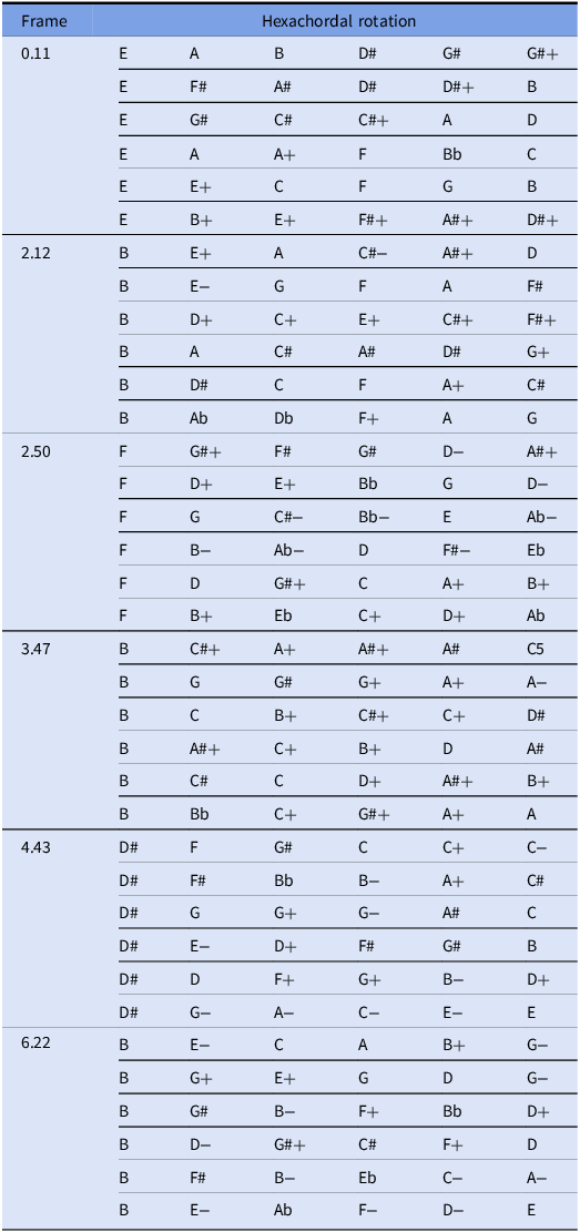
While the frequencies indicated pitches in specific octaves, they were further treated as pitch classes, considering the notes as symbols of equal value across every octave (Rahn Reference Rahn1980). Looking at the list obtained with the aim of establishing pitch series for composing, a selection process was applied discarding the rows that presented repeated pitch classes or missing values (due to the lack of enough light contrast in certain images) and favouring those rows that presented more potential in compositional terms, such as diversity of intervals, internal tensions, harmonic colour and melodic lines. This resulted in the selection of six hexachordal series of microtonal pitch classes. Using a microtonal system served as a means of tuning into subtler nuances of brightness shown in the images.

It is worth noting that translating data into sound entails a selective process that corresponds to Barad’s (Reference Barad2007: 19) description of apparatuses as ‘measurement interactions’ through which ‘certain properties become determinate’. For instance, in the sonification process deployed by Diaz-Merced et al. (Reference Diaz-Merced, Candey, Brickhouse, Schneps, Mannone, Brewster and Kolenberg2012: 135), temporal fluctuation information was first transcribed to a cluster to then derive a pitch that changed temporarily according to phase, frequency and duration variations. Based on Bohr’s research, Barad’s critique interrogates traditional science’s epistemological understanding of the phenomena being observed as determined before the observational experience and highlights how apparatuses model the data observed. In making aesthetics choices that foreground the compositional apparatus employed, the aural reconfiguration I propose here explores a Baradian approach to apparatuses as specific material-discursive practices that ‘reconfigure spatiality and temporality as well as the traditional notions of dynamics’ (Barad Reference Barad2007: 146).

Table 6 shows the selected series including their corresponding time code as well as five permutations of each series developed as rotational arrays, a technique much employed by Stravinsky in his serial works. The five permutations keep the same pitch class as the first of the array and replicate the integers in the initial array successively starting by the interval between the second and third pitch classes (Straus Reference Straus1999: 47). This operation is expressed in the algorithms below.

$$\eqalign{ & {\rm{The \;first \;row \;is \;represented \;as}}:x = \left( {x1,x2,x3,x4,x5,x6} \right). \cr & {\rm{The \;intervals \;of \;that \;row \;are \;represented \;as}}:d1\; = x1 \to x2,d2\; \cr & = x2 \to x3,d3\; = x3 \to x4,d4\; = x4 \to x5,d5\; = x5 \to x6,\cr & d6\; = x6 \to x1. \cr & {\rm{The \;cyclic \;interval \;vector \;of \;row \;x \;is \;D}}\left( {\rm{x}} \right) = \left( {d1,d2,d3,d4,d5,d6} \right). \cr & {\rm{The \;rows \;below \;are \;y}},z,a,{\rm{b \;and }}\;c,{\rm{represented \;as}}:\cr & y = \left( {y1,y2,y3,y4,y5,y6} \right). \cr & {\rm{An \;anchor \;condition \;applies \;so \;that }}\;x1 = y1 = z1 = a1 = b1 = c1. \cr & {\rm{The \;intervals \;of \;the \;rows \;below \;are \;obtained \;from \;the \;rotated \;vector}}: \cr}$$

$$\eqalign{ & {D}\left( y \right) = \left( {d2,d3,d4,d5,d6,d1} \right) \cr & {D}\left( z \right) = \left( {d3,d4,d5,d6,d1,d2} \right) \cr & {D}\left( a \right)\; = \;\left( {d4,d5,d6,d1,d2,d3} \right) \cr & {D}\left( b \right) = \left( {d5,d6,d1,d2,d3,d4} \right) \cr & {D} {\unicode{x00A9}} = \left( {d6,d1,d2,d3,d4,d5} \right) \cr}$$

Table 6.

Virtual galaxy simulation, hexachords with their rotational arrays

Table 6. Long description

A table showing hexachordal rotations with their corresponding time codes and permutations. The table has 6 rows and 7 columns. Column headers are Frame and Hexachordal rotation. Row labels are time codes in seconds. Values are musical notes and their permutations. Row 1: Frame 0.11, Hexachordal rotation E, A, B, D#, G#, G#+. Row 2: Frame 0.11, Hexachordal rotation E, F#, A#, D#, D#+, B. Row 3: Frame 0.11, Hexachordal rotation E, G#, C#, C#+, A, D. Row 4: Frame 0.11, Hexachordal rotation E, A, A+, F, Bb, C. Row 5: Frame 0.11, Hexachordal rotation E, E+, C, F, G, B. Row 6: Frame 0.11, Hexachordal rotation E, B+, E+, F#+, A#+, D#+. Row 7: Frame 2.12, Hexachordal rotation B, E+, A, C#-, A#+, D. Row 8: Frame 2.12, Hexachordal rotation B, E-, G, F, A, F#. Row 9: Frame 2.12, Hexachordal rotation B, D+, C+, E+, C#+, F#+. Row 10: Frame 2.12, Hexachordal rotation B, A, C#, A#, D#, G+. Row 11: Frame 2.12, Hexachordal rotation B, D#, C, F, A+, C#. Row 12: Frame 2.12, Hexachordal rotation B, Ab, Db, F+, A, G. Row 13: Frame 2.50, Hexachordal rotation F, G#+, F#, G#, D-, A#+. Row 14: Frame 2.50, Hexachordal rotation F, D+, E+, Bb, G, D-. Row 15: Frame 2.50, Hexachordal rotation F, G, C#-, Bb-, E, Ab-. Row 16: Frame 2.50, Hexachordal rotation F, B-, Ab-, D, F#-, Eb. Row 17: Frame 2.50, Hexachordal rotation F, D, G#+, C, A+, B+. Row 18: Frame 2.50, Hexachordal rotation F, B+, Eb, C+, D+, Ab. Row 19: Frame 3.47, Hexachordal rotation B, C#+, A+, A#+, A#, C5. Row 20: Frame 3.47, Hexachordal rotation B, G, G#, G+, A+, A-. Row 21: Frame 3.47, Hexachordal rotation B, C, B+, C#+, C+, D#. Row 22: Frame 3.47, Hexachordal rotation B, A#+, C+, B+, D, A#. Row 23: Frame 3.47, Hexachordal rotation B, C#, C, D+, A#+, B+. Row 24: Frame 3.47, Hexachordal rotation B, Bb, C+, G#+, A+, A. Row 25: Frame 4.43, Hexachordal rotation D#, F, G#, C, C+, C-. Row 26: Frame 4.43, Hexachordal rotation D#, F#, Bb, B-, A+, C#. Row 27: Frame 4.43, Hexachordal rotation D#, G, G+, G-, A#, C. Row 28: Frame 4.43, Hexachordal rotation D#, E-, D+, F#, G#, B. Row 29: Frame 4.43, Hexachordal rotation D#, D, F+, G+, B-, D+. Row 30: Frame 4.43, Hexachordal rotation D#, G-, A-, C-, E-, E. Row 31: Frame 6.22, Hexachordal rotation B, E-, C, A, B+, G-. Row 32: Frame 6.22, Hexachordal rotation B, G+, E+, G, D, G-. Row 33: Frame 6.22, Hexachordal rotation B, G#, B-, F+, Bb, D+. Row 34: Frame 6.22, Hexachordal rotation B, D-, G#+, C#, F+, D. Row 35: Frame 6.22, Hexachordal rotation B, F#, B-, Eb, C-, A-.

These algorithms were embedded throughout the composed work, where only the pitches in the series and its permutations were used during the time spanning between the initial time code from which the values were extracted and the next one. Each array was explored in both vertical and horizontal dispositions, without any exhaustion rules for repeating the pitch classes.

I organised the formal structure of the piece into three main sections based on three distinct patterns of particle motion. I crafted the music material of each section drawing upon Lachenmann’s (Reference Lachenmann and Häusler1996) sound types. The first section, shown in Figure 6, engages with Lachenmann’s second sound type, which explores the timbral qualities of a relatively stationary spectrum. This sound type consists of stable vertical superpositions of pitches and partials, with the pitches notated in the score excerpt in Figure 6 belonging to the first hexachordal array (the score is transposed).

Figure 6.

Virtual Galaxy Simulation score, page 3.

The second section corresponds to Lachenmann’s fourth sound type, a textural compound of large, sustained sounds and short, isolated events that evolve constantly at a micro-level. Figure 7 shows an excerpt from the second section in which I employed pitch classes from the second hexachordal array.

Figure 7.

Virtual Galaxy Simulation score, page 7.

The third section (see Figure 8) is scored to the spiral-wave phase, the most intense stage of particle motion. The texture explored corresponds to Lachenmann’s third sound type, described as fluctuation and characterised as a gradually expanding texture that appears less complex at the macro-level than its internal development actually is. Lachenmann (Reference Lachenmann and Häusler1996) explains that the timbral, textural and fluctuating types explored here belong to a broader group characterised by internal processes that shape time from the inside out, in contrast to the attack-and-decay sound type, which consists of a cadential gesture. In the development of their internal structures, the three sound types examined in this work adapt their formal duration to the ways in which the musical material unfolds. Such temporal transformations shape audiences’ perception of time, corresponding, I suggest, to the visual and aural narrative of galaxy formation presented in this piece. As the cosmological processes involved in galaxy formations unfold over timescales far exceeding human perception, galaxy formation simulations attempt to speculatively overcome the limitations of direct observation. While it is not possible to portray the formation of a galaxy at the same temporal rate at which it occurs, the sound types employed shape temporal perception in ways that evoke the stretching of time within the dynamics of particle motion being visualised and auralised, inviting audiences to attune to more-than-human temporal experiences.

Figure 8.

Virtual Galaxy Simulation score, page 11.

While the instrumental parts enact the diverse components of galactic matter, I sought to articulate the narrative voice of this galaxy formation story in the electronics part. Exploring timbral possibilities around voice-like sounds, the electronics’ material was created from recordings of breathy sounds, a cat’s purring captured with contact microphones, as well as recordings of the instrumental parts. These recordings were spectrally modified through the selection and expansion of partials, as well as through the synthesis of sounds derived from spectral analysis of the recordings. In each section, the electronics reinforce the main texture, adding further timbral layers. The octophonic spatialisation was designed in synchrony with the motion in the image, creating bursts of isolated sounds and spiral rotations across the eight-speaker array. While Havelková (Reference Havelková2021) discusses the immediacy of the voice as arising from the bodily presence of operatic singing, in this work I examine a comparable sense of narrative immediacy through the omnipresent effect of octophonic sound diffusion, relying on the combined cinematic environment of video projection and octophonic electronics to foreground the simulation of galaxy formation as a humanly narrated story.

Bird’s kinetic literature

The work discussed in this section engages with Le Guin’s notion of kinetic art proposed in The Author of the Acacia Seeds, where the most effective translation of penguin language is accomplished by a ballet company (515–516). Therolinguists advance their ability to read their sea literature upon understanding that penguins are birds that ‘fly in water’ (515). Le Guin’s therolinguists read a semantic dimension in the materiality of the penguins’ motion and its traces in the water in line with the ‘account of materiality as an agentive and productive factor in its own right’ proposed by Barad (Reference Barad2007: 225). The task of transcribing bird motion bears surprising resemblances with studies of bird flight conserved in manuscripts written by Leonardo da Vinci (Reference da Vinci1452–Reference da Vinci1519), in which he sketched observations of birds in motion, drawing conclusions on the physical mechanics that enabled their flight which expressed precise dynamic relations between body weight, gravity, responsive movement, and specific winds. Following Le Guin’s suggestion that birds’ literature is a collective one, and so appropriately performed by a ballet, I thought of the orchestra as the most suitable medium for sonically reconfiguring da Vinci’s observations of bird flight, which led me to compose Volo degli Uccelli (Birds’ Flight) (2024/25) for orchestra. I therefore considered da Vinci’s sketches as graphic matrixes for devising textures on the orchestral score. As shown in Figure 9, I mapped the orchestral instruments as single lines across the page intersected by replications of the birds’ flight sketches. The bird’s body parts are spread across the instrumental forces so that the right wing lays on the strings section, the left wing on the woodwinds, the torso, tail and head on the brass section and the traces of winds on the percussion section. Orchestral textural changes informed by non-human motion have been explored in Saariaho’s (Reference Saariaho2005) Asteroid 4179: Toutatis, in which she explores the peculiar shape and rotation cycle of this asteroid creating constantly fluctuating textures (Saariaho Reference Saariaho2024).

Figure 9.

Volo degli Uccelli orchestral texture sketches.

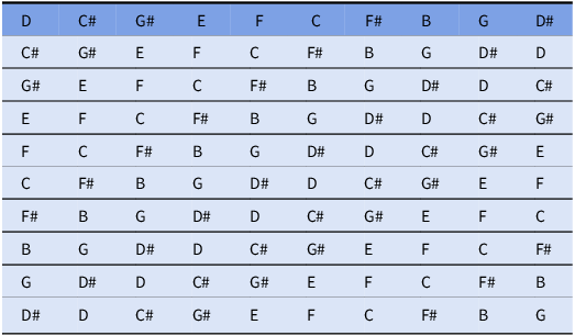
Da Vinci uses alphabetic points in his sketches to illustrate motion directions and relative distances. I listed the letters used in the sketches I addressed in this orchestral work, which add up to ten different letters: A-B-C-D-E-F-G-M-N-P. I used this list of letters as a matrix to create a series of ten pitch classes assigned to each of the letters, presented in the top row of Table 7. I then transcribed the series vertically to the furthest left column and completed the series in each row, creating rotations that offer combinations of the notes within a Latin square matrix. The rotations of the series created within this Latin square follow the algorithm below, similar to that of Table 2.

$$\matrix{ {{\rm{If }}\,L\,\left( {i,j} \right){{\rm\, is\, the\, entry\, in\, row}\,i, {\rm column}\,j, {\rm where\, }}i,j \in \left\{ {0,\; \ldots, \;9} \right\},} \cr {{\rm{and }}\,S\,\left\{ {s0,\; \ldots, s9} \right\}{\rm{\, is\, the\, ordered\, series\, in\, the\, first\, row, then}}} \cr {L\,\left( {i,j} \right)\; = S\left( {i + j} \right)\,{\rm{ mod\, 10}}} \cr }$$

Table 7.

Volo degli Uccelli, pitch class series permutated in a Latin square

Table 7. Long description

The table displays a 10-by-10 grid containing musical note names on a light blue background with gray dividing lines and a darker blue top row. Each cell contains one musical note, including natural notes and sharp notes. Reading from left to right, the first row is D, C sharp, G sharp, E, F, C, F sharp, B, G, and D sharp, followed by rows beginning with C sharp, G sharp, E, F, C, F sharp, B, G, and D sharp respectively, with the note sequences shifting cyclically across subsequent rows. The grid contains the notes C, C sharp, D, D sharp, E, F, F sharp, G, G sharp, and B, while A and A sharp do not appear.

Each row contains the first row shifted left by i places. Upon reaching the tenth note, ‘mod 10’ at the end of the calculation continues the sequence again from the first note of the series. The 9 rotations obtained are shown in Table 7.

I creatively embedded these algorithms in the compositional process by way of developing musical material tracing vertical, horizontal and diagonal routes across the square, completing melodic or harmonic assemblies of ten pitches or less.

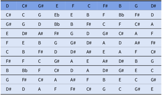
In Table 8, I developed transpositions of the intervals of the series in the top row, taking each note in the top series as the first note of each row below, and applying the succession of intervals in the initial series starting from that first note. This procedure is expressed in the following algorithm.

$${\matrix{ {{\rm{If\, again\, }}L\left( {i,j} \right)\,{\rm{ is\, the\, entry\, in\, row\, }}i,{\rm{ column\, }}j,} \\ {{\rm{ where\, }}i,j \in \left\{ {0,\; \ldots, \;9} \right\},S\left\{ {s0,\; \ldots, s9} \right\}{\rm{\, is\, the \,ordered\, series\,}}} \\ {{\rm{in\, the\, first\, row, and\, to\, measure\, the\, interval\, from\, }}} \\ {{\rm the\, first\, notes\,1\, the\, calculation\, is }}\,sj-s0,\;\\ \,{\rm then}\, L\left( {i,j} \right)\; = Si + \;\left( {sj-s0} \right)\;\left( {{\rm{mod \,12}}} \right)} }$$

Table 8.

Volo degli Uccelli, pitch class rotations

Table 8. Long description

A table with 11 rows and 12 columns displaying pitch class rotations. The columns are labeled with musical notes: D, C sharp, G sharp, E, F, C, F sharp, B, G, D sharp. Each row represents a transposition of the intervals of the series in the top row, starting from a different note. Row 1: D, C sharp, G, E flat, E, B, F, B flat, F sharp, D, A. Row 2: G sharp, G, D, B flat, B, F sharp, C, F, C sharp, A, E. Row 3: E, D sharp, A sharp, F sharp, G, D, G sharp, C sharp, A, F, F. Row 4: F, E, B, G, D, G sharp, D sharp, A, D, A sharp, F sharp. Row 5: C, B, F sharp, D, D sharp, A sharp, E, A, F, C sharp, C. Row 6: F sharp, F, C, G sharp, A, E, A sharp, D sharp, B, G, D. Row 7: B, B flat, F, C sharp, D, A, D sharp, G sharp, E, C, G. Row 8: G, F sharp, C sharp, A, A sharp, F, B, E, C, G sharp, D. Row 9: D sharp, D, A, F, F sharp, C sharp, G, C, G sharp, E, B. Row 10: D, A, F, F sharp, C sharp, G, C, G sharp, E, B, G sharp.

The first note of row i is Si. All subsequent notes are obtained by adding the intervals as in the original top row, measured from the first note to each column. Pitch values are delimited according to modulo 12 because the series belongs to a chromatic system. The 9 transpositions of the series obtained are shown in Table 8.

Finally, I assigned rhythmic cells to the alphabetic series, which I then permutated in a Latin square matrix, shown in Table 9. These permutations follow the same algorithmic pattern as those presented in Table 7. I also assembled these rhythmic combinations similarly to how I navigated the musical possibilities that emerge from the rotations in Table 7, tracing vertical, horizontal and diagonal routes (and combinations of these) across the Latin square to obtain rhythmic sequences and superpositions, which are viewable in the excerpt of the score shown in Figure 10. Material from the pitch series can also be found in this excerpt, such as the material in the bassoon line starting in bar 19, which uses the pitch classes in the third row of Table 9 in an iterative order.

Table 9.

Volo degli Uccelli, rhythmic series in a Latin square matrix

Table 9. Long description

Panel A: A musical score with rhythmic patterns arranged in a grid. The grid consists of multiple rows and columns filled with various musical notes and rests. Each cell in the grid contains a unique combination of notes and rests, creating a complex rhythmic series. The patterns follow a specific algorithmic structure, with vertical, horizontal, and diagonal routes forming different rhythmic sequences and superpositions. The score includes various musical symbols such as quarter notes, eighth notes, and rests, arranged in a structured manner.

Figure 10.

Volo degli Uccelli score, pages 5–6.

Figure 10. Long description

Panel A: The left page of the musical score features multiple staves for different instruments including percussion, woodwinds, brass, and strings. Each staff has musical notes and various annotations such as dynamics and articulation marks. Specific instruments like Tenor Drum, Glockenspiel, and bowed percussion are indicated. Panel B: The right page continues the musical score with similar staves and annotations. It includes measures with detailed musical notation, dynamics, and articulation marks. The score is divided into sections with measure numbers indicated at the top of each section.

The orchestral score of Volo degli Uccelli presents kinetic positions of bird flight successively evolving through a narrative of ascent, kinetic changes in response to wind alterations, and descent. Measures 18 to 23 on pages 5 to 6, featured in Figure 10, present a frontal view of a bird with wings open to each side. Measures 24 to 28 on page 6, also in Figure 10, present an overhead view of a bird adopting an asymmetric disposition of the wings as a dynamic response to asymmetric wind blows which ensures balance preservation. By way of auralising traces of bird flight, the daily struggles of animal displacement through gravitational and meteorological constraints are sonically narrated with the aim of telling a life story focused on animal life, one that attempts to decipher traces of non-human movement as traces of meaning.

Listening to sea waste

I could not finish this article without considering a work that tells a life story addressing the current state of our planet. This section discusses the sound installation The Listening Canvas (2024) exhibited at the international conference on NIME 2024, in which I invite audiences to engage in tactic and aural interactions to sonically reconfigure the impact of waste on sea waters. A vast range of human activities including industrial production, agriculture, mining and urban waste are causes of water contamination, disposing industrial discharges, animal refuse, litter, heavy metals, oil, grease, plastic detritus, household chemicals and urban runoff in rivers, lakes and ocean waters (Yadav Reference Yadav2024: 1246). The Listening Canvas consists of a canvas displaying recycled materials usually found in water waste (plastics, fabrics, cardboard, metals) surrounded by foam sheets hanging inside fishing nets (see Figure 11).

Figure 11.

The Listening Canvas exhibited at NIME.

The installation enables a two-sided experience in which listening and sound-making are equally encouraged. Audiences are invited to produce sounds by touching the canvas with their hands or with plant stems and leaves provided as well as by vocalising towards the canvas. These gestures are captured by piezo transducers placed behind the canvas. The acoustic sounds captured are processed in real time, through both the amplification of untreated noise and frequency analysis followed by transposition into an audible range, which triggers sound synthesis based on the resulting pitches. The algorithm involved in the sound treatments applied is presented below.

First, the frequencies (f) of the acoustic sounds captured are shifted up two octaves, which amount to 24 semitones, plus 3 semitones, which equals to a total of 27 semitones. This step is applied by the plugin shown in Figure 12.

$$f \cdot {2^{27/12}} = f\prime$$

Next, the transposed frequencies are converted to MIDI notes, represented in the formula below as pitch (p). To capture as many live interactions as possible during the exhibition, this audio to MIDI conversion process is applied up to 4 times within a 20-millisecond window. Previously shifting the frequencies to a higher range optimises this process, since higher frequencies have shorter periods and can therefore be estimated more reliably within such short analysis window.

$$p^\prime \; = \;69\; + \;12{\rm{ lo}}{{\rm{g}}_2}\left( {f^\prime /440} \right)$$

Figure 12.

Reaper settings for pitch transposition before sound synthesis.

Once transposed and converted to MIDI notes, the pitches obtained are transposed down by both 13 and 7 semitones, creating a lower, denser pitch spectrum that triggers sound synthesis within an audible range. This step is expressed below.

$$\left\{ {p^{\prime_1},p^{\prime_2}} \right\}\; = \;\left\{ {p^\prime\; - \;13,p^\prime\;- \;7} \right\}$$

A digital synthesiser finally outputs the synthesised sounds. To diffuse these sounds, the MIDI notes are translated back into frequencies through the algorithm shown below.

$${f_{1,2}} = \;440 \cdot {2^{\left( {p^\prime1,2\;- \;69} \right)/12}}$$

Both the captured acoustic sounds and the synthesised sounds are diffused through transducers attached to the hanging foam sheets. The Listening Canvas’ exploration of sound display through transducers placed on resonating materials engages with David Tudor’s (Reference Tudor1973) sound installation Rainforest IV, which introduced this technique creating sculptural speakers. This ground-breaking sound art piece suggests a sonic exploration of apparently static objects navigating their agential sonic properties across the exhibition space as if they were the flora of an imaginary, surrealist rainforest. The use of piezoelectric transducers for capturing ultrasound has been discussed by Barad (Reference Barad2007: 221) as an interface to the body when considering the technical and semantic procedures of volumic echography, in which a computer is used to store and integrate the two-dimensional images captured by the transducer to produce a three-dimensional mapping of the scanned organ’s volume. This is comparable to the processes deployed in the live electronics, where infrasound is transposed to higher ranges (Figure 12) and then transposed down to lower yet audible ranges before triggering sound synthesis. The amplification of acoustic sounds combined with the transformation of inaudible sounds into audible ones produces an aural image of the materiality of sea waste perceivable through human interplay. Barad (Reference Barad2007: 220) warns that technoscientific discourses surrounding echography technology ‘seduce the viewer into thinking that the representation of the object is isomorphic with the object itself’. This assumption corresponds to the semantic practices discussed above in relation to the dissemination of cosmological observations, which overlook the impact material-semiotic apparatuses have on the phenomena disseminated. Through the embedment of the algorithms described, The Listening Canvas foregrounds the apparatuses of real-time sound production employed and facilitates listening experiences that encourage reflections on water pollution.

This work draws connections with Leonora Carrington’s (Reference Carrington1976) surrealist novel The Hearing Trumpet, in which an elderly woman is given a hearing trumpet to be able to communicate with those around her, which is presented as an initiation device within a surrealist found object approach, while listening is presented as a transformative action. Upon being able to listen, the vulnerable woman becomes able to form alliances with elderly people in her care home. Together, at the end of the novel, they achieve an ecofeminist utopian ecology that entails new fairer forms of coexistence among humans and other species.

By exploring the sounds created with both vegetal and disposable synthetic materials and by using a sonic and visual representation of water as backdrop, audiences are invited to participate in reconfigurations that challenge binary divides between the water perceived as nature and waste perceived as the byproduct of culture, towards a new material-semantic ecology enabled through the hypermedial setting of the installation. The Listening Canvas aims to engage audiences in experimental sound-making and active listening practices (see Luciana Perc Reference Perc2024b to view a video documentation of audiences engaging with the installation exhibited at NIME) and thus invites them to collectively participate in the construction of meanings through the examination of sound as a switchboard (Havelková Reference Havelková2021). The organic and synthetic materials used to produce sounds within the canvas’ surface are explored sonically in a way that fosters different modes of listening, disrupting existing narratives on water pollution to think new forms of accountability and responsible action. The installation works as a reconfiguring device that facilitates sonic matter and meaning production. Yet, the artwork does not claim to facilitate a direct dialogue with the earth that may show us the way forward. As Haraway (Reference Haraway2016: 44) reminds us:

The earth has regenerative resources, on which human prospects of survival and better living conditions rely. Haraway’s (Reference Haraway2016) call to stay with the trouble seeks to foster such regenerative processes which are more worth thinking than apocalyptic futures projections.