1 Introduction
Vortices in geophysical flows have received much attention, especially in the oceans, due to their important role in energy and scalar transports as well as mixing. For example, Meddies (Mediterranean eddies) are formed by warm salty water flowing from the Mediterranean sea into the Atlantic ocean. These mesoscale vortices can live years travelling in the ocean (Armi et al. Reference Armi, Hebert, Oakey, Price, Richardson, Rossby and Ruddick1989; Hobbs Reference Hobbs2007; Ménesguen et al. Reference Ménesguen, Hua, Carton, Klingelhoefer, Schnrle and Reichert2012a ). Their thickness is typically 1 km and their diameter typically 100 km (Richardson, Bower & Zenk Reference Richardson, Bower and Zenk2000). Similar eddies, called Ulleung eddies, are formed by warm northward and cold southward currents in the East/Japan sea. Once formed, the eddies are trapped in the Ulleung basin near Ulleung island (Chang et al. Reference Chang, Teague, Lyu, Perkins, Lee, Watts, Kim, Mitchell, Lee and Kim2004). These eddies are also pancake shaped with both warm and cold cores, and a lifetime of approximately a couple of years. The characteristics of these mesoscale eddies are important because they can greatly affect the fisheries (Kim et al. Reference Kim, Yang, Kim, Shin, Park, Yoo and Hyun2012). There exist actually many observations of such mesoscale eddies in other places: for example, Reddies (Red Sea eddies) (Meschanov & Shapiro Reference Meschanov and Shapiro1998) and Swoddies (Slope water oceanic eddies) (Pingree & Le Cann Reference Pingree and Le Cann1992; Carton Reference Carton2001; Carton et al. Reference Carton, Le Cann, Serpette and Dubert2013).
Idealized models of these vortices have been studied experimentally and numerically with a layered density stratification (Saunders Reference Saunders1973; Griffiths & Linden Reference Griffiths and Linden1981; Ikeda Reference Ikeda1981; Helfrich & Send Reference Helfrich and Send1988; Ripa Reference Ripa1991; Hopfinger & van Heijst Reference Hopfinger and van Heijst1993; Dewar & Killworth Reference Dewar and Killworth1995; Killworth, Blundell & Dewar Reference Killworth, Blundell and Dewar1997; Dewar, Killworth & Blundell Reference Dewar, Killworth and Blundell1999; Baey & Carton Reference Baey and Carton2002; Benilov Reference Benilov2003; Thivolle-Cazat, Sommeria & Galmiche Reference Thivolle-Cazat, Sommeria and Galmiche2005; Aubert et al.
Reference Aubert, Le Bars, Le Gal and Marcus2012; Lahaye & Zeitlin Reference Lahaye and Zeitlin2015) as well as in continuously stratified fluids (Dritschel, de la Torre Juárez & Ambaum Reference Dritschel, de la Torre Juárez and Ambaum1999; Reinaud, Dritschel & Koudella Reference Reinaud, Dritschel and Koudella2003; Nguyen et al.
Reference Nguyen, Hua, Schopp and Carton2012; Lazar et al.
Reference Lazar, Stegner, Caldeira, Dong, Didelle and Viboud2013a
; Lazar, Stegner & Heifetz Reference Lazar, Stegner and Heifetz2013b
; Hua et al.
Reference Hua, Ménesguen, Le Gentil, Schopp, Marsset and Aiki2013; Dritschel & McKiver Reference Dritschel and McKiver2015). Saunders (Reference Saunders1973) studied experimentally the stability of a vortex produced by releasing a cylindrical volume of fluid into a fluid with a lighter density placed on a turntable rotating at a constant speed. The spreading of the denser fluid at the bottom resulted in an anticyclonic vortex which was stable when the Burger number
 $Bu=({\it\delta}{\it\rho}g/{\it\rho})H/f^{2}R^{2}>1.8$
, where
 ${\it\delta}{\it\rho}$
is the density difference between the two fluids,
 $g$
the gravity,
 $H$
the height,
 $f$
the Coriolis parameter and
 $R$
the radius of the inner cylinder. In contrast, when
 $Bu<1.8$
, azimuthal disturbances grew on the vortex due to baroclinic instability. The azimuthal wavenumber
 $m$
scaled like
 $m\sim 1.8Bu^{-1/2}$
, i.e. the wavelength scales like the Rossby deformation radius
 $R_{d}=({\it\delta}{\it\rho}gH/{\it\rho})^{1/2}/f$
, and the smallest wavenumber observed was an
 $m=1$
wandering mode of the whole vortex. Similar observations have been later reported by Griffiths & Linden (Reference Griffiths and Linden1981) and Thivolle-Cazat et al. (Reference Thivolle-Cazat, Sommeria and Galmiche2005) when the inner cylindrical volume of fluid is less dense and has smaller depth than the surrounding fluid. However, the
 $m=1$
wandering mode has not been observed for these surface vortices. Numerical simulations performed by Verzicco, Lalli & Campana (Reference Verzicco, Lalli and Campana1997) found good agreement with the results of Griffiths & Linden (Reference Griffiths and Linden1981). Griffiths & Linden (Reference Griffiths and Linden1981) also conducted experiments when a fluid is injected at constant flux into a rotating fluid with a different constant density or with a continuous stratification. In this case, barotropic instability first developed and then baroclinic instability as the anticyclonic vortex grew in size. In the case of continuous stratification, they also observed layers above and below the vortex core that they attributed to the viscous–diffusive instability of McIntyre (Reference McIntyre1970). A similar instability was observed by Hedstrom & Armi (Reference Hedstrom and Armi1988) but non-axisymmetric disturbances were not observed to grow in contrast to Griffiths & Linden (Reference Griffiths and Linden1981). Hedstrom & Armi (Reference Hedstrom and Armi1988) have also shown that the aspect ratio and velocity field were in good agreement with the prediction of the lens model of Gill (Reference Gill1981) in quasi-geostrophic fluids. Recently, Aubert et al. (Reference Aubert, Le Bars, Le Gal and Marcus2012) and Hassanzadeh, Marcus & Le Gal (Reference Hassanzadeh, Marcus and Le Gal2012) have proposed and validated a universal law for the vortex aspect ratio valid in general stratified-rotating fluids which takes into account a density gradient in the vortex core.
Many numerical and theoretical results exist on the stability of axisymmetric vortices for various vortex profiles in one-layer rotating shallow-water fluids (Ford Reference Ford1994; Stegner & Dritschel Reference Stegner and Dritschel2000), two-layer quasi-geostrophic fluids (Ikeda Reference Ikeda1981; Flierl Reference Flierl1988; Helfrich & Send Reference Helfrich and Send1988; Benilov Reference Benilov2003) or two-layer rotating shallow-water fluids for Rossby numbers smaller than unity (Ripa Reference Ripa1991; Dewar & Killworth Reference Dewar and Killworth1995; Killworth et al.
Reference Killworth, Blundell and Dewar1997; Dewar et al.
Reference Dewar, Killworth and Blundell1999; Baey & Carton Reference Baey and Carton2002) In one layer, vortices with a monotonic potential vorticity may be subjected to a radiative instability while, for isolated vortices, the barotropic shear instability is dominant but tends to be stabilized as the Burger number
 $Bu$
decreases. In contrast, two-layer vortices are increasingly unstable to baroclinic instability as
 $Bu$
decreases. Baroclinic instability is also enhanced (stabilized) when the vortices in each layer are counter-rotating (co-rotating). Recently, Nguyen et al. (Reference Nguyen, Hua, Schopp and Carton2012) have conducted a numerical stability analysis of a pancake vortex in continuously stratified quasi-geostrophic fluids. In the case of a Gaussian angular velocity in both radial and vertical directions, they found that the dominant instability when the Burger number
 $Bu=N^{2}{\it\Lambda}^{2}/f^{2}R^{2}<1$
(where
 $N$
is the Brunt–Väisälä frequency,
 ${\it\Lambda}$
the half-thickness of the vortex and
 $R$
its radius) is generally a baroclinic instability with an azimuthal wavenumber
 $m=2$
. However, for very small
 $Bu<0.1$
, higher azimuthal modes become dominant. For
 $Bu>1$
, the dominant mode is an
 $m=1$
barotropic mode anti-symmetric with respect to the mid-horizontal plane. Such a bending mode is similar to the ‘internal instability’ evidenced by Gent & McWilliams (Reference Gent and McWilliams1986) on columnar isolated vortices in quasi-geostrophic fluids. Yim & Billant (Reference Yim and Billant2015) have shown that this instability, which we will call ‘Gent–McWilliams instability’ herein, is due to the presence of a critical point where the angular velocity of the vortex is equal to the phase speed of the disturbances and where the radial gradient of base vorticity is positive. Hua et al. (Reference Hua, Ménesguen, Le Gentil, Schopp, Marsset and Aiki2013) have performed nonlinear simulations of the dynamics of a lens-shaped vortex in continuously stratified quasi-geostrophic fluids. In addition to the development of the asymmetric disturbances, they evidenced layering in the vicinity of critical levels where the azimuthal phase speed of the disturbances equal the angular velocity of the vortex.
The stability of axisymmetric vortices for larger Rossby numbers has been also investigated (Smyth & McWilliams Reference Smyth and McWilliams1998; Billant, Colette & Chomaz Reference Billant, Colette and Chomaz2004; Lazar et al.
Reference Lazar, Stegner, Caldeira, Dong, Didelle and Viboud2013a
,Reference Lazar, Stegner and Heifetz
b
; Lahaye & Zeitlin Reference Lahaye and Zeitlin2015). In the case of a columnar Gaussian vortex in inviscid, continuously stratified-rotating fluids, Smyth & McWilliams (Reference Smyth and McWilliams1998) have shown that centrifugal instability becomes dominant over the Gent–McWilliams instability and shear instability for sufficiently high Rossby number. Lazar et al. (Reference Lazar, Stegner, Caldeira, Dong, Didelle and Viboud2013a
,Reference Lazar, Stegner and Heifetz
b
) studied experimentally and theoretically the stability of vortices in linearly stratified and rotating viscous fluids with respect to the axisymmetric centrifugal instability. Taking into account the leading viscous effects, which scale like
 $k^{2}$
for large vertical wavenumber
 $k$
, they obtained analytic predictions for the most amplified vertical wavenumber and the marginal stability curves in terms of the Burger, Ekman and Rossby numbers. Lahaye & Zeitlin (Reference Lahaye and Zeitlin2015) have investigated the linear stability and nonlinear dynamics of anticyclones with a
 ${\it\alpha}$
-Gaussian profile in a two-layer shallow-water model. They have shown that asymmetric centrifugal instabilities become more unstable than the axisymmetric mode as the Rossby number
 $Ro$
decreases or as the Burger number
 $Bu$
increases. For small
 $Ro$
or high
 $Bu$
, the barotropic shear instability is dominant. Billant et al. (Reference Billant, Colette and Chomaz2004) have carried out experiments on a columnar counter-rotating vertical vortex pair in a linearly stratified and rotating fluid. They have shown that the dominant centrifugal instability developing on the anticyclone is non-axisymmetric with an azimuthal wavenumber
 $m=1$
for moderate Rossby number and small Froude number.
Recently, Yim & Billant (Reference Yim and Billant2016) (hereafter referred as to part 1) have analysed the stability of a Gaussian pancake vortex in continuously stratified non-rotating fluids. Instabilities similar to those of columnar vortices have been observed. Centrifugal instability is almost independent of the aspect ratio due to its short-wavelength nature and occurs when the buoyancy Reynolds number
 $ReF_{h}^{2}$
is sufficiently large:
 $ReF_{h}^{2}>10^{3}$
, where
 $F_{h}={\it\Omega}_{0}/N$
is the Froude number based on the maximum angular velocity
 ${\it\Omega}_{0}$
and
 $Re={\it\Omega}_{0}R^{2}/{\it\nu}$
, where
 ${\it\nu}$
is the viscosity. Shear instability can develop when
 $F_{h}/{\it\alpha}<0.5$
where
 ${\it\alpha}={\it\Lambda}/R$
is the aspect ratio of the pancake vortex. In addition, instabilities specific to pancake vortices can exist: baroclinic instability when
 $F_{h}/{\it\alpha}\geqslant 1.46$
and gravitational instability when
 $F_{h}/{\it\alpha}\geqslant 1.5$
.
In this paper, we will continue these stability analyses in the case of a stratified-rotating fluid in order to link the infinite Rossby number limit (part 1) to the small Rossby number limit (Nguyen et al.
Reference Nguyen, Hua, Schopp and Carton2012). We show that some instabilities can be traced continuously from the stratified non-rotating limit to the quasi-geostrophic limit, while new types of instabilities arise as
 $Ro$
is varied.
The paper is organized as follows: the stability problem and methods are formulated in § 2. The effect of the Rossby number is investigated in § 3 while the effects of the other parameters (
 $F_{h},{\it\alpha}$
and
 $Re$
) are studied in § 4. In § 5, the energetics of some instabilities are analysed in detail in order to characterize their origin. Conditions of existence for shear instability, Gent–McWilliams instability and baroclinic instability are derived in § 6, § 7 and § 8, respectively. Finally, § 9 summarizes the domains of existence of each type of instability in the parameter space (
 $F_{h}/{\it\alpha}$
,
 $Ro$
) and (
 $Bu,Ro$
).
2 Problem formulation
The problem formulation is the same as in part 1 except that the fluid is not only stably stratified but also rotating about the vertical axis at rate
 $f/2$
. For clarity, the main steps of the methods are nevertheless recalled here.
2.1 The base state
As in Nguyen et al. (Reference Nguyen, Hua, Schopp and Carton2012) and part 1, we consider an axisymmetric pancake vortex with angular velocity
 $$\begin{eqnarray}{\it\Omega}(r,z)={\it\Omega}_{0}\text{e}^{-(r^{2}/R^{2}+z^{2}/{\it\Lambda}^{2})},\end{eqnarray}$$
where (
 $r,{\it\theta},z$
) are cylindrical coordinates with
 $z$
pointing upward,
 $R$
the radius,
 ${\it\Lambda}$
the typical half-thickness and
 ${\it\Omega}_{0}$
the maximum angular velocity. The radial and vertical inviscid momentum equations under the Boussinesq approximation for such steady base flow are
 $$\begin{eqnarray}\displaystyle & \displaystyle -r{\it\Omega}^{2}-fr{\it\Omega}=-\frac{1}{{\it\rho}_{0}}\frac{\partial p_{t}}{\partial r}, & \displaystyle\end{eqnarray}$$
 $$\begin{eqnarray}\displaystyle & \displaystyle 0=-\frac{1}{{\it\rho}_{0}}\frac{\partial p_{t}}{\partial z}-\frac{g}{{\it\rho}_{0}}{\it\rho}_{t}, & \displaystyle\end{eqnarray}$$
where
 $p_{t}$
and
 ${\it\rho}_{t}$
are the total pressure and density, respectively,
 $g$
is the gravity and
 ${\it\rho}_{0}$
a constant reference density. Combining (2.2) and (2.3) gives the thermal wind equation
 $$\begin{eqnarray}\frac{\partial {\it\rho}_{t}}{\partial r}=-\frac{{\it\rho}_{0}}{g}\frac{\partial }{\partial z}(r{\it\Omega}^{2}+fr{\it\Omega}),\end{eqnarray}$$
yielding
 $$\begin{eqnarray}{\it\rho}_{t}={\it\rho}_{0}+\bar{{\it\rho}}(z)+{\it\rho}_{b}(r,z),\end{eqnarray}$$
with
 $\bar{{\it\rho}}(z)=-N^{2}{\it\rho}_{0}z/g$
where
 $N=\sqrt{-g/{\it\rho}_{0}(\text{d}\bar{{\it\rho}}/\text{d}z)}$
is the Brunt–Väisälä frequency which is assumed constant and
 $$\begin{eqnarray}{\it\rho}_{b}(r,z)=-z\frac{{\it\rho}_{0}}{\text{g}}\left(\frac{R}{{\it\Lambda}}\right)^{2}\left({\it\Omega}+f\right){\it\Omega},\end{eqnarray}$$
is the density field associated with the vortex.
2.2 Linearized equations
We subject this vortex to infinitesimal perturbations of velocity
 $\boldsymbol{u}^{\prime }=[u_{r}^{\prime },u_{{\it\theta}}^{\prime },u_{z}^{\prime }]$
, pressure
 $p^{\prime }$
and density
 ${\it\rho}^{\prime }$
written as
 $$\begin{eqnarray}[u_{r}^{\prime },u_{{\it\theta}}^{\prime },u_{z}^{\prime },p^{\prime },{\it\rho}^{\prime }]=\left[u_{r}(r,z),u_{{\it\theta}}(r,z),u_{z}(r,z),{\it\rho}_{0}p(r,z),\frac{{\it\rho}_{0}}{g}{\it\rho}(r,z)\right]\text{e}^{-\text{i}{\it\omega}t+\text{i}m{\it\theta}}+\text{c.c}.,\end{eqnarray}$$
where
 $m$
is the azimuthal wavenumber and
 ${\it\omega}={\it\omega}_{r}+\text{i}{\it\omega}_{i}$
, with
 ${\it\omega}_{r}$
the frequency and
 ${\it\omega}_{i}$
the growth rate. The linearized Navier–Stokes equations under the Boussinesq approximation are
 $$\begin{eqnarray}\displaystyle & \displaystyle -\text{i}({\it\omega}-m{\it\Omega})u_{r}-(2{\it\Omega}+f)u_{{\it\theta}}=-\frac{\partial p}{\partial r}+{\it\nu}\left({\rm\nabla}^{2}u_{r}-\frac{1}{r^{2}}u_{r}-\frac{2}{r^{2}}\text{i}mu_{{\it\theta}}\right)\!, & \displaystyle\end{eqnarray}$$
 $$\begin{eqnarray}\displaystyle & \displaystyle -\text{i}({\it\omega}-m{\it\Omega})u_{{\it\theta}}+({\it\zeta}+f)u_{r}+\frac{\partial r{\it\Omega}}{\partial z}u_{z}=-\frac{\text{i}m}{r}p+{\it\nu}\left({\rm\nabla}^{2}u_{{\it\theta}}-\frac{1}{r^{2}}u_{{\it\theta}}+\frac{2}{r^{2}}\text{i}mu_{r}\right)\!, & \displaystyle\end{eqnarray}$$
 $$\begin{eqnarray}\displaystyle & \displaystyle -\text{i}({\it\omega}-m{\it\Omega})u_{z}=-\frac{\partial p}{\partial z}-{\it\rho}+{\it\nu}{\rm\nabla}^{2}u_{z}, & \displaystyle\end{eqnarray}$$
 $$\begin{eqnarray}\displaystyle & \displaystyle -\text{i}({\it\omega}-m{\it\Omega}){\it\rho}+\frac{g}{{\it\rho}_{0}}\frac{\partial {\it\rho}_{b}}{\partial r}u_{r}+\frac{g}{{\it\rho}_{0}}\frac{\partial {\it\rho}_{b}}{\partial z}u_{z}=N^{2}u_{z}+{\it\kappa}{\rm\nabla}^{2}{\it\rho}, & \displaystyle\end{eqnarray}$$
 $$\begin{eqnarray}\displaystyle & \displaystyle \frac{1}{r}\frac{\partial ru_{r}}{\partial r}+\frac{1}{r}\text{i}mu_{{\it\theta}}+\frac{\partial u_{z}}{\partial z}=0, & \displaystyle\end{eqnarray}$$
where
 ${\it\zeta}=(1/r)\partial r^{2}{\it\Omega}/\partial r$
is the vertical vorticity,
 ${\it\nu}$
the viscosity and
 ${\it\kappa}$
the diffusivity of the stratifying agent. The viscous and diffusive damping of the base state are neglected in (2.8)–(2.12) as classically done in stability analyses (Drazin & Reid Reference Drazin and Reid1981). This assumption is valid as long as the time taken by the perturbations to grow to finite amplitude is small compared to the viscous decay time of the base flow. The problem is governed by five non-dimensional numbers: aspect ratio (
 ${\it\alpha}$
), Froude number (
 $F_{h}$
), Rossby number (
 $Ro$
), Reynolds number (
 $Re$
), Schmidt number (
 $Sc$
), defined as follows:
 $$\begin{eqnarray}{\it\alpha}=\frac{{\it\Lambda}}{R},\quad F_{h}=\frac{{\it\Omega}_{0}}{N},\quad Ro=\frac{2{\it\Omega}_{0}}{f},\quad Re=\frac{{\it\Omega}_{0}R^{2}}{{\it\nu}},\quad Sc=\frac{{\it\nu}}{{\it\kappa}}.\end{eqnarray}$$
The Schmidt number is set to
 $Sc=1$
throughout the paper. In part 1, the effect of the Schmidt number has been studied and shown to affect only the axisymmetric mode of centrifugal instability. The equations (2.8)–(2.12) in the inviscid and non-diffusive limit are non-dimensionalized in appendix A and shown to reduce to the quasi-geostrophic equation when
 $Ro\ll 1$
and
 $F_{h}\ll 1$
whatever the aspect ratio
 ${\it\alpha}$
. For this reason, even if we consider here aspect ratios not as small as in the oceans, the quasi-geostrophic regime will be reached for sufficiently small Rossby and Froude numbers.
As explained in part 1, equations (2.8)–(2.12) are discretized with finite element methods using FreeFEM++ (Hecht Reference Hecht2012; Garnaud Reference Garnaud2012) in the domain
 $0\leqslant r\leqslant R_{\mathit{max}}$
and
 $-Z_{\mathit{max}}\leqslant z\leqslant Z_{\mathit{max}}$
. The size is taken as
 $R_{\mathit{max}}\geqslant 10R$
and
 $Z_{\mathit{max}}=5{\it\Lambda}$
. These sizes are slightly different compared to part 1 because some modes are more sensitive to radial confinement in the presence of background rotation. The mesh is adapted to the base flow so that the mesh is finer (
 ${\sim}0.001R$
) inside the vortex core than outside (
 ${\sim}0.1R$
). The boundary conditions at
 $r=0$
are
 $u_{r}=u_{{\it\theta}}=0$
for
 $m=0$
,
 $u_{z}=p={\it\rho}=0$
for
 $m=1$
and
 $\boldsymbol{u}=p={\it\rho}=0$
for
 $m\geqslant 2$
. At the other boundaries,
 $R=R_{\mathit{max}}$
and
 $z=\pm Z_{\mathit{max}}$
, all the perturbations are imposed to vanish:
 $\boldsymbol{u}=p={\it\rho}=0$
. The matrix version of (2.8)–(2.12) built by FreeFEM++ is then solved by means of an iterative Krylov–Schur scheme and a shift-invert method using the SLEPc and PETSc libraries (Hernandez, Roman & Vidal Reference Hernandez, Roman and Vidal2005; Garnaud Reference Garnaud2012; Garnaud et al.
Reference Garnaud, Lesshafft, Schmid and Huerre2013; Balay et al.
Reference Balay, Abhyankar, Adams, Brown, Brune, Buschelman, Eijkhout, Gropp, Kaushik and Knepley2014; Roman et al.
Reference Roman, Campos, Romero and Tomas2015). More details can be found in part 1. The limit
 ${\it\alpha}\rightarrow \infty$
corresponding to a columnar vortex has been solved by means of a Chebyshev collocation spectral method (Antkowiak & Brancher Reference Antkowiak and Brancher2004).
In appendix B, it is shown that the equations (2.8)–(2.12) in the quasi-geostrophic and inviscid limits (
 $Ro\rightarrow 0,F_{h}\rightarrow 0,Re=\infty$
) can be solved by separation of variables and a shooting method for
 $Bu=Ro^{2}{\it\alpha}^{2}/(4F_{h}^{2})=1$
. Hence, this particular case has been used as a validation test for the code based on FreeFEM++ and SLEPc. The eigenvalues obtained by the two numerical methods are in good agreement (see appendix B).
3 Overview of the effect of the Rossby number
We first present an overview of the effect of the Rossby number for the azimuthal wavenumbers
 $m=0,1,2$
starting from the strongly stratified non-rotating limit (
 $F_{h}<1$
and
 $Ro=\infty$
) previously studied in part 1. This will enable us to connect the purely stratified limit to the quasi-geostrophic limit studied by Nguyen et al. (Reference Nguyen, Hua, Schopp and Carton2012). Throughout the paper, the exploration of the parameter space will be restricted to the region stable to gravitational instability, i.e. where the total density gradient
 $$\begin{eqnarray}\frac{\partial {\it\rho}_{t}}{\partial z}=-\frac{{\it\rho}_{0}N^{2}}{g}+\frac{\partial {\it\rho}_{b}}{\partial z},\end{eqnarray}$$
is everywhere negative. This condition can be rewritten in the form
 $$\begin{eqnarray}\frac{F_{h}}{{\it\alpha}}<c_{g}(Ro),\end{eqnarray}$$
where
 $c_{g}$
is a constant depending on the Rossby number. When
 $Ro=\infty$
,
 $c_{g}=\text{e}^{3/4}/\sqrt{2}\simeq 1.5$
whereas for
 $Ro\ll 1$
,
 $c_{g}=\text{e}^{3/4}\sqrt{Ro}/2\simeq 1.06\sqrt{Ro}$
. However, the constant
 $c_{g}$
cannot be expressed analytically for arbitrary
 $Ro$
. The minimum of the Richardson number
 $$\begin{eqnarray}Ri={\displaystyle \frac{-{\displaystyle \frac{g}{{\it\rho}_{0}}}{\displaystyle \frac{\partial {\it\rho}_{t}}{\partial z}}}{\left({\displaystyle \frac{\partial u_{{\it\theta}}}{\partial z}}\right)^{2}}},\end{eqnarray}$$
is always larger than
 $1/4$
when the condition (3.2) is satisfied, meaning that a shear instability due to the vertical shear should not occur in the region stable to gravitational instability (Negretti & Billant Reference Negretti and Billant2013).
Growth rate (
 ${\it\omega}_{i}/{\it\Omega}_{0}$
) and frequency (
 ${\it\omega}_{r}/{\it\Omega}_{0}$
) spectra for
 $m=0$
for different Rossby numbers
 $Ro$
: (a)
 $Ro=\infty$
, (b)
 $Ro=20$
and (c)
 $Ro=-10$
for
 $F_{h}=0.5$
and
 $Re=10\,000$
. Discrete symbols (○: for symmetric and

 ${\it\alpha}=0.5$
and thick continuous lines (

 ${\it\alpha}=\infty$
).

Real part of the radial velocity perturbation Re(
 $u_{r}$
) of centrifugal instability (CI): (a) mode
 $(0,1)$
for
 $Ro=20$
and (b) mode
 $(0,3)$
for
 $Ro=-10$
indicated in figure 1 (
 $m=0,F_{h}=0.5,{\it\alpha}=0.5,Re=10\,000$
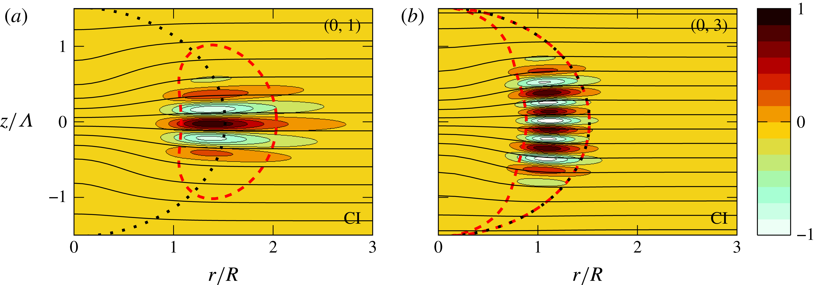
). The quasi-horizontal lines are isopycnals of the base density field. The dotted line indicates the extension of the base flow by showing the contour where
 ${\it\Omega}=0.1{\it\Omega}_{0}$
. The dashed line indicates the contour where the Rayleigh discriminant
 ${\it\Phi}$
vanishes.
3.1 Azimuthal wavenumber
 $m=0$

For
 $m=0$
, it has been found in part 1 that only a centrifugal instability exists in a stratified fluid when the buoyancy Reynolds number
 $ReF_{h}^{2}$
is sufficiently high. This remains true when the Rossby number is varied. Figure 1 shows two examples of spectra for
 $Ro=20$
and
 $Ro=-10$
together with the one for
 $Ro=\infty$
, all for the same set of parameters:
 ${\it\alpha}=0.5,F_{h}=0.5$
and
 $Re=10\,000$
. The unstable modes are shown by symbols and are labelled
 $(m,i)$
where
 $i$
is the mode number. For each point, there exist actually two modes with different symmetry with respect to the mid-plane
 $z=0$
: anti-symmetric (○) and symmetric (

 $Ro$
but these variations are consistent with the spectra of the most unstable mode of a columnar vortex for the same Reynolds, Froude and Rossby numbers (grey continuous lines). Some examples of modes are shown in figure 2. The modes are localized inside the region delimited by a dashed line where the Rayleigh discriminant
 $$\begin{eqnarray}{\it\Phi}=\left.\frac{1}{r^{3}}\frac{\partial }{\partial r}\left(r^{4}\left({\it\Omega}+\frac{f}{2}\right)^{2}\right)\right|_{{\it\rho}_{t}},\end{eqnarray}$$
Maximum growth rate of centrifugal instability for
 $m=0$
as a function of
 $Ro$
for a pancake vortex for
 ${\it\alpha}=0.5$
(


 $F_{h}=0.5$
and
 $Re=10\,000$
. The dashed grey line (

 $m=0$
:
 $\sqrt{-\text{min}({\it\phi})}$
. The vertical shaded region is the region unstable to gravitational instability. The upper
 $x$
-axis indicates the corresponding value of square root of the Burger number
 $\sqrt{Bu}$
.

is negative. The radial derivative in (3.4) is taken along constant density surfaces as specified by the generalisation of the Rayleigh criterion to baroclinic vortices (Solberg Reference Solberg1936; Eliassen & Kleinschmidt Reference Eliassen, Kleinschmidt and Bartels1957). The minimum of
 ${\it\Phi}$
is located on the symmetry plane
 $z=0$
whatever
 $Ro$
but the region of negative
 ${\it\Phi}$
has a bean shape for
 $Ro>\exp (2)=7.39$
and a croissant shape (extending to the axis at
 $z=\sqrt{\ln (-Ro)}$
) for
 $Ro<-1$
. The number of oscillations of the modes along the vertical increases with the mode number but there is always a single oscillation along the radial direction for the parameters of figure 1. The variation of the growth rate of the most unstable mode as a function of
 $Ro$
for
 ${\it\alpha}=0.5,F_{h}=0.5$
and
 $Re=10\,000$
is summarized in figure 3 (dashed line with circles). Centrifugal instability is stabilized for small Rossby number in the range
 $-3.5<Ro<17$
. A similar evolution of the maximum growth rate is observed for a columnar vortex (grey continuous line). As shown in part 1, the growth rate of the centrifugal instability can be predicted using the asymptotic formula of Billant & Gallaire (Reference Billant and Gallaire2005) for large axial wavenumber
 $k$
for a columnar vortex with the addition of the leading viscous term as in Lazar et al. (Reference Lazar, Stegner and Heifetz2013b
):
 $$\begin{eqnarray}{\it\omega}={\it\omega}^{(0)}-\frac{{\it\omega}^{(1)}N}{k}-\text{i}{\it\nu}k^{2},\end{eqnarray}$$
where
 $$\begin{eqnarray}\displaystyle & \displaystyle {\it\omega}^{(0)}=m{\it\Omega}(r_{0})+\text{i}\sqrt{-{\it\phi}(r_{0})}, & \displaystyle\end{eqnarray}$$
 $$\begin{eqnarray}\displaystyle & \displaystyle {\it\omega}^{(1)}=\frac{(2n+1)\text{i}}{2\sqrt{2}}\sqrt{\frac{{\it\phi}^{\prime \prime }(r_{0})-2m^{2}{\it\Omega}^{\prime }(r_{0})^{2}+2\text{i}m\sqrt{-{\it\phi}(r_{0})}{\it\Omega}^{\prime \prime }(r_{0})}{-{\it\phi}(r_{0})}}\sqrt{1-\frac{{\it\phi}(r_{0})}{N^{2}}}, & \displaystyle\end{eqnarray}$$
with
 $n$
a non-negative integer,
 ${\it\phi}=(2{\it\Omega}+f)({\it\zeta}+f)$
and
 $r_{0}$
is given by
 $$\begin{eqnarray}\displaystyle {\it\phi}^{\prime }(r_{0})=-2\text{i}m{\it\Omega}^{\prime }(r_{0})\sqrt{-{\it\phi}(r_{0})}. & & \displaystyle\end{eqnarray}$$
The maximum growth rate predicted by (3.5) for
 $F_{h}=0.5$
and
 $Re=10\,000$
is shown by the dashed grey line in figure 3. It is close to the maximum growth rate for both columnar and pancake vortices. We can remark that the maximum growth rate for
 $F_{h}=0.5$
and
 $Re=10\,000$
is approximately three times smaller than the theoretical upper limit for the growth rate of a centrifugal instability which is
 $\sqrt{-\min ({\it\phi})}$
for
 $m=0$
(solid line in figure 3) and which is attained in the limit
 $k\rightarrow \infty$
and
 ${\it\nu}\rightarrow 0$
. Note that
 $\min ({\it\phi})=\min ({\it\Phi})$
since
 ${\it\Phi}$
is minimum on the symmetry plane
 $z=0$
.
3.2 Azimuthal wavenumber
$m=1$

A spectrum for
 $m=1$
for a large Rossby number
 $Ro=20$
and
 ${\it\alpha}=0.5$
,
 $F_{h}=0.5$
and
 $Re=10\,000$
is displayed in figure 4(b). The spectrum of a columnar vortex for the same parameter is also shown by a continuous grey line for comparison. These spectra are qualitatively similar to those for
 $Ro=\infty$
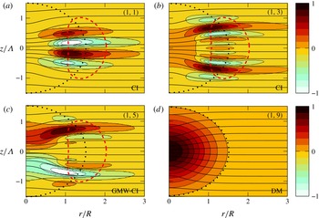
(shown in figure 4(a) for reference) in which three types of modes have been identified in part 1. From this basis, we can easily classify the different modes in figure 4(b). The series of modes ((1, 1)–(1, 4), (1, 6)–(1, 8)) correspond to centrifugal instability. The eigenmodes differ again by the number of oscillations along the vertical (compare modes (1, 1) and (1, 3) in figure 5) but they have all a single oscillation along the radial direction. They are localized near the region where
 ${\it\Phi}$
is negative and they tend to be aligned along the base isopycnals (figure 5
a,b). The mode (1, 5) in figure 4(b) corresponds to a mixed Gent–McWilliams–centrifugal instability since it exhibits both the characteristics of centrifugal and Gent–McWilliams instabilities (figure 5
c). The latter instability, which is also called the internal instability, bends the vortex and is due to the presence of a critical layer where
 ${\it\Omega}={\it\omega}_{r}$
and where the vertical vorticity radial gradient is positive (Gent & McWilliams Reference Gent and McWilliams1986; Smyth & McWilliams Reference Smyth and McWilliams1998; Yim & Billant Reference Yim and Billant2015). The mode (1, 9) is almost neutral with zero frequency for large
 $Re$
. Its radial velocity perturbation (figure 5
d) is almost identical to the angular velocity of the base flow, implying that it displaces the vortex without deforming it. As shown in part 1, this mode corresponds to the displacement mode originating from the translational invariance. In § 4.1, it will be shown that the instability of the displacement mode is due to viscous effects.
Growth rate (
 ${\it\omega}_{i}/{\it\Omega}_{0}$
) and frequency (
 ${\it\omega}_{r}/{\it\Omega}_{0}$
) spectra for
 $m=1$
for different Rossby numbers
 $Ro$
: (a)
 $Ro=\infty$
, (b)
 $Ro=20$
, (c)
 $Ro=-10$
(d)
 $Ro=5$
, (e)
 $Ro=2$
and (f)
 $Ro=1.43$
for
 $F_{h}=0.5$
and
 $Re=10\,000$
. Discrete symbols (○: for symmetric and

 ${\it\alpha}=0.5$
and thick continuous lines (

 ${\it\alpha}=\infty$
).

Real part of the radial velocity perturbation Re(
 $u_{r}$
) of centrifugal instability (CI) (a) mode (1, 1) and (b) mode (1, 3), (c) mixed Gent–McWilliams–centrifugal instability (GMW-CI) (1, 5) and (d) the displacement mode (DM) (1, 9) for
 $Ro=20$
(figure 4
b) (
 $m=1,{\it\alpha}=0.5,F_{h}=0.5,Re=10\,000$
). The quasi-horizontal lines are isopycnals. The dotted line indicates the extension of the base flow by showing the contour where
 ${\it\Omega}=0.1{\it\Omega}_{0}$
. The dashed line indicates the contour where the Rayleigh discriminant
 ${\it\Phi}$
vanishes.

Real part of the radial velocity perturbation Re(
 $u_{r}$
) of (a) centrifugal instability
 $(1,1)$
and (b) Gent–McWilliams instability (GMWI) (1, 5) for
 $Ro=-10$
(figure 4
c) (
 $m=1,{\it\alpha}=0.5,F_{h}=0.5,Re=10\,000$
). The quasi-horizontal lines are isopycnals. The dotted line indicates the extension of the base flow by showing the contour where
 ${\it\Omega}=0.1{\it\Omega}_{0}$
. The dashed line indicates the contour where the Rayleigh discriminant
 ${\it\Phi}$
vanishes.

A similar spectrum is observed for
 $Ro=-10$
(figure 4
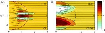
c) except that there is a clear separation between centrifugal and Gent–McWilliams instabilities. This is similar to the columnar vortex case (grey solid line) where Gent–McWilliams instability and centrifugal instability correspond to two distinct growth rate peaks for negative Rossby numbers in contrast to positive Rossby numbers (Yim & Billant Reference Yim and Billant2015). The structure of centrifugal instabilities (figure 6
a) is similar to those for
 $Ro=20$
(figure 5
a,b). Gent–McWilliams instability (figure 6
b) is localized in the vortex core and corresponds more clearly to a bending of the vortex as a whole than for
 $Ro=20$
(figure 5
c) where the mixed Gent–McWilliams–centrifugal mode tends to concentrate at the top and bottom of the pancake vortex.
When the absolute value of the Rossby number is further decreased, the centrifugal instability disappears since
 ${\it\Phi}>0$
everywhere when
 $-1\leqslant Ro\leqslant 7.39$
and only the Gent–McWilliams instability remains, as exemplified in figure 4(d) for
 $Ro=5$
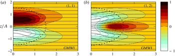
. In this case, there are three unstable Gent–McWilliams modes and the first two are displayed in figure 7. The first one (figure 7
a) is similar to the one previously shown in figure 6(b) for
 $Ro=-10$
while the second one exhibits one more oscillation along the vertical and is thus symmetric (figure 7
b). There is still also the displacement mode ((1, 4) in figure 4
d) with a very weak frequency and growth rate. All these modes are close to the spectrum of a columnar vortex shown by the grey solid line (figure 4
d). The maximum frequency of the unstable branch of the columnar vortex is
 ${\it\omega}_{r}={\it\Omega}_{0}\text{e}^{-2}=0.135{\it\Omega}_{0}$
. This corresponds to the maximum frequency for which the gradient of the vertical vorticity
 ${\it\zeta}^{\prime }(r_{c})$
is positive at the critical radius
 $r_{c}$
where
 ${\it\Omega}(r_{c})={\it\omega}_{r}$
.
Real part of the radial velocity perturbation Re(
 $u_{r}$
) of Gent–McWilliams instability (GMWI): (a) mode
 $(1,1)$
and (b) mode
 $(1,2)$
for
 $Ro=5$
(figure 4
d) (
 $m=1,{\it\alpha}=0.5,F_{h}=0.5,Re=10\,000$
). The quasi-horizontal lines are isopycnals. The dotted line indicates the extension of the base flow by showing the contour where
 ${\it\Omega}=0.1{\it\Omega}_{0}$
.

Real part of the radial velocity perturbation Re(
 $u_{r}$
) of the mixed baroclinic–Gent–McWilliams instability (BGMWI): mode
 $(1,1)$
for
 $Ro=2$
(figure 4
e) (
 $m=1,{\it\alpha}=0.5,F_{h}=0.5,Re=10\,000$
). The quasi-horizontal lines are isopycnals. The dotted line indicates the extension of the base flow by showing the contour where
 ${\it\Omega}=0.1{\it\Omega}_{0}$
.

Real part of the radial velocity perturbation Re(
 $u_{r}$
) of the (a) mode
 $(1,1)$
, (b) mode
 $(1,2)$
, (c) mode
 $(1,3)$
and (d) mode
 $(1,6)$
for
 $Ro=1.43$
(figure 4
f) (
 $m=1,{\it\alpha}=0.5,F_{h}=0.5,Re=10\,000$
). The quasi-horizontal lines are isopycnals. The dotted line indicates the extension of the base flow by showing the contour where
 ${\it\Omega}=0.1{\it\Omega}_{0}$
. The double dotted dashed line (


So far, all the unstable modes observed for a pancake vortex derive from those for a columnar vortex. However, when the Rossby number is further decreased to
 $Ro=2$
(figure 4
e) and then to
 $Ro=1.43$
(figure 4
f), all the unstable modes for pancake vortices have no counterparts in columnar vortices except the displacement mode near the origin ((1, 4) in figure 4(e) and (1, 7) in figure 4
f). For
 $Ro=2$
(figure 4
e), the most unstable mode (1, 1) has a frequency larger than
 $0.135{\it\Omega}_{0}$
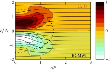
but is still close to the spectra of the columnar vortex. The structure of this mode (figure 8
a) is similar to Gent–McWilliams instability for
 $Ro=5$
(figure 7
a) but it tends to be distorted near
 $r=R$
. In § 5, we will show that the energy source of this mode is the potential energy of the base flow instead of the kinetic energy. For this reason, we shall call it mixed baroclinic–Gent–McWilliams instability. Two other modes start also to be observed near the frequency
 ${\it\omega}_{r}=0.25{\it\Omega}_{0}$
(figure 4
e) but they are weakly unstable. In contrast, for
 $Ro=1.43$
(figure 4
f), there are many modes around this frequency and their growth rate is much larger. The leading mode (1,1) corresponds in fact to baroclinic–Gent–McWilliams mode whose frequency and growth rate have increased until merging with the series of modes aligned near the frequency
 ${\it\omega}_{r}=0.25{\it\Omega}_{0}$
. A selection of these modes are depicted in figure 9. The first mode (1,1) shows some similarities with the one for
 $Ro=2$
(figure 8) but it is clearly more concentrated in the vortex core
 $r/R_{0}\leqslant 0.5$
and is maximum at a slightly higher vertical level
 $z/{\it\Lambda}=\pm 0.7$
. The next modes are similar but exhibit more radial oscillations (figure 9
b–d) with still two vertical oscillations, i.e. one per half-vertical plane. Similar modes have been observed in stratified non-rotating fluids (part 1) when the isopycnal deformations are sufficiently strong and have been attributed to baroclinic instability (BI). The isopycnals are indeed more and more distorted when the Rossby number decreases for given aspect ratio and Froude number. The isopycnals even overturn, i.e.
 $\max (\partial {\it\rho}_{t}/\partial z)>0$
, when
 $Ro\leqslant 1.3$
for
 ${\it\alpha}=0.5$
and
 $F_{h}=0.5$
. In quasi-geostrophic fluids, a necessary condition for baroclinic instability is the sign change of the potential vorticity gradient along the isopycnals (Charney & Stern Reference Charney and Stern1962; Eliassen Reference Eliassen1983; Hoskins, McIntyre & Robertson Reference Hoskins, McIntyre and Robertson1985; Ménesguen, McWilliams & Molemaker Reference Ménesguen, McWilliams and Molemaker2012b
):
 $$\begin{eqnarray}\left.{\displaystyle \frac{\partial {\it\Pi}}{\partial r}}\right|_{{\it\rho}_{t}}={\displaystyle \frac{\partial {\it\Pi}}{\partial r}}-{\displaystyle \frac{\partial {\it\Pi}}{\partial z}}{\displaystyle \frac{{\displaystyle \frac{\partial {\it\rho}_{t}}{\partial r}}}{{\displaystyle \frac{\partial {\it\rho}_{t}}{\partial z}}}}=0,\end{eqnarray}$$
where
 ${\it\Pi}=({\it\zeta}+f)\partial {\it\rho}_{t}/\partial z-r\partial {\it\Omega}/\partial z\partial {\it\rho}_{t}/\partial r$
is the potential vorticity of the base flow. The double dotted dashed line in figure 9 shows where
 $\partial {\it\Pi}/\partial r|_{{\it\rho}_{t}}=0$
. As can be seen, the modes develop in the vicinity of this line suggesting that they are due to baroclinic instability. In this respect, the leading mode (1,1) (figure 9
a) is not different from the following modes (figure 9
b–d) and could be equally classified as baroclinic. However, we will continue to call it baroclinic–Gent–McWilliams mode since it derives continuously from Gent–McWilliams instability as
 $Ro$
increases. A detailed study of these baroclinic modes will be conducted in § 8.
(a) Maximum growth rates and (b) corresponding frequencies of the different types of instability as a function of
 $Ro$
for
 $m=1$
,
 ${\it\alpha}=0.5,F_{h}=0.5$
and
 $Re=10\,000$
: centrifugal instability


 $x$
axis indicates the corresponding value of the square root of the Burger number
 $\sqrt{Bu}$
. The shaded region is gravitationally unstable.

The effect of the Rossby number on the growth rate and frequency of the most unstable modes of each instability for
 $m=1$
is summarized in figure 10. As already seen for
 $m=0$
, centrifugal instability (dashed line with circles) is stabilized for small negative
 $Ro\gtrsim -2$
. For positive Rossby number, centrifugal instability transforms continuously into the Gent–McWilliams instability (dashed line with filled triangle) when
 $Ro\lesssim 7$
(Yim & Billant Reference Yim and Billant2015). The growth rate of the mixed Gent–McWilliams–centrifugal instability (dashed line with open triangle) is almost constant for large Rossby number. For negative Rossby number, the Gent–McWilliams instability stabilizes around
 $Ro\sim -2$
as for the centrifugal instability. For positive Rossby number, the growth rate of the Gent–McWilliams instability decreases as the Rossby number decreases and becomes minimum for
 $Ro\simeq 2$
corresponding to a Burger number
 $Bu=({\it\alpha}Ro/2F_{h})^{2}\equiv (N{\it\Lambda}/fR)^{2}$
of approximately unity, as indicated in the upper
 $x$
axis in figure 10. Below this Rossby number, the frequency (figure 10
b) increases beyond the cutoff frequency
 ${\it\omega}_{r}=0.135{\it\Omega}_{0}$
above which the Gent–McWilliams instability no longer exists in the case of a columnar vortex (Yim & Billant Reference Yim and Billant2015). Simultaneously, the growth rate again increases and the instability becomes a mixed baroclinic–Gent–McWilliams instability (dashed line with star). For smaller Rossby number, the instability merges with the pure baroclinic instability (dashed line with diamond) with a growth rate increasing dramatically as
 $Ro$
decreases. However, the frequency saturates at
 ${\it\omega}_{r}\simeq 0.25{\it\Omega}_{0}$
. The growth rate of the displacement mode (dashed line with square) remains very low for any Rossby number.
(a) Maximum growth rate and (b) corresponding frequency of centrifugal instability (

 ${\it\alpha}=0.5$
) (

 $Ro$
for
 $m=1,F_{h}=0.5$
and
 $Re=10\,000$
. The dashed grey line shows the maximum of the asymptotic growth rate (3.5). The dotted line indicates the Gent–McWilliams instability.

Similar results have been obtained by Nguyen et al. (Reference Nguyen, Hua, Schopp and Carton2012) in quasi-geostrophic fluids except that the centrifugal instability is absent since
 $Ro\ll 1$
. Thus, they have reported for
 $m=1$
only two modes that they distinguish by their symmetry: a symmetric and an anti-symmetric mode. When the Burger number is of order unity or larger, the symmetric mode corresponds to the displacement mode herein and the anti-symmetric mode is similar to the Gent–McWilliams most unstable mode. In contrast, when
 $Bu$
is small, the symmetric and anti-symmetric modes correspond to the leading baroclinic modes herein (BGMWI or BI depending on
 $Bu$
). The growth rate of the anti-symmetric mode is minimum for
 $Bu=1$
as in figure 10 when the transition between the Gent–McWilliams and baroclinic–Gent–McWilliams instabilities occur.
Finally, figure 11 shows that the maximum growth rate and corresponding frequency of the centrifugal instability for pancake (dashed line with circle) and columnar (grey continuous line) vortices are close. The maximum growth rate and associated frequency predicted by (3.5) is also represented by a dashed line. It underestimates the observed growth rate of both pancake and columnar vortices for positive Rossby number. This discrepancy comes from the smooth transition between Gent–McWilliams and centrifugal instabilities as
 $Ro$
varies.
Growth rate (
 ${\it\omega}_{i}/{\it\Omega}_{0}$
) and frequency (
 ${\it\omega}_{r}/{\it\Omega}_{0}$
) spectra for
 $m=2$
for different Rossby numbers
 $Ro$
: (a)
 $Ro=\infty$
, (b)
 $Ro=20$
, (c)
 $Ro=0.8$
and (d)
 $Ro=0.25$
for
 $F_{h}=0.5$
and
 $Re=10\,000$
. Discrete symbols (○: for symmetric and

 ${\it\alpha}=1.2$
and thick continuous lines (

 ${\it\alpha}=\infty$
).

In summary, for
 $m=1$
, the baroclinic–Gent–McWilliams instability dominates when
 $Ro$
is small and the centrifugal instability takes over when
 $Ro$
is large. In between, there exists a Gent–McWilliams instability for positive
 $Ro$
. For negative
 $Ro$
, the centrifugal instability is always dominant. Although only one particular set of parameters (
 ${\it\alpha}=0.5,F_{h}=0.5$
and
 $Re=10\,000$
) has been presented, we shall see in § 4 that this picture is typical of other parameter combinations in the strongly stratified regime with moderate and strong rotation.
3.3 Azimuthal wavenumber
$m=2$

Finally, we present the effect of the Rossby number on the stability of the azimuthal wavenumber
 $m=2$
for the set of parameters:
 ${\it\alpha}=1.2,F_{h}=0.5$
and
 $Re=10\,000$
. Note that the aspect ratio is changed compared to
 $m=0$
and
 $m=1$
in order to show more typical examples of spectra. In the strongly stratified non-rotating case (part 1), two instabilities have been found: a centrifugal instability for sufficiently large buoyancy Reynolds number
 $ReF_{h}^{2}$
and a shear instability when
 $F_{h}/{\it\alpha}\leqslant 0.5$
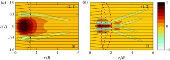
. These correspond to the modes (2, 1)–(2, 2) and (2, 3), respectively in figure 12(a). When the Rossby number is decreased, a scenario similar to the one described for
 $m=1$
occurs. Centrifugal instability becomes less dominant for moderate Rossby number (see figure 12(b) for
 $Ro=20$
) and disappears for small Rossby number (see figure 12(c) for
 $Ro=0.8$
) since
 ${\it\Phi}>0$
for
 $-1<Ro<7.39$
. An example of the structure of a centrifugal mode for
 $Ro=20$
is depicted in figure 13(b). In contrast, a baroclinic instability appears for small Rossby number (modes (2, 1)–(2, 4) in figure 12(d) for
 $Ro=0.25$
). As for
 $m=1$
(figure 9), the baroclinic modes differ by the number of oscillations in the radial direction and by their symmetry with respect to the mid-plane
 $z=0$
(not shown).
Real part of the radial velocity perturbation Re(
 $u_{r}$
) of (a) shear instability (SI)
 $(2,1)$
and (b) centrifugal instability (CI)
 $(2,2)$
for
 $Ro=20$
(figure 12
b) (
 $m=2,{\it\alpha}=1.2,F_{h}=0.5,Re=10\,000$
). The quasi-horizontal lines are isopycnals. The dotted line indicates the extension of the base flow by showing the contour where
 ${\it\Omega}=0.1{\it\Omega}_{0}$
. The dash dotted line in (a) shows the inflection radius
 $r_{I}$
where
 ${\it\zeta}^{\prime }(r_{I})=0$
. The dashed line in (b) indicates the contour where the Rayleigh discriminant
 ${\it\Phi}$
vanishes.

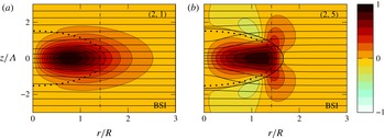
Real part of the radial velocity perturbation Re(
 $u_{r}$
) of the mixed baroclinic–shear instability (BSI) (a) mode
 $(2,1)$
for
 $Ro=0.8$
(figure 12
c) and (b) mode
 $(2,5)$
for
 $Ro=0.25$
(figure 12
d) (
 $m=2,{\it\alpha}=1.2,F_{h}=0.5,Re=10\,000$
). The quasi-horizontal lines are isopycnals. The dotted line indicates the extension of the base flow by showing the contour where
 ${\it\Omega}=0.1{\it\Omega}_{0}$
. The dash dotted line shows the inflection radius
 $r_{I}$
where
 ${\it\zeta}^{\prime }(r_{I})=0$
. The solid line in (b) show the critical layer where
 ${\it\omega}_{r}=m{\it\Omega}(r,z)$
.

(a) Maximum growth rates and (b) corresponding frequencies of the different types of instabilities as a function of
 $Ro$
for
 $m=2,{\it\alpha}=1.2$
,
 $F_{h}=0.5$
and
 $Re=10\,000$
: centrifugal instability


 $x$
axis indicates the corresponding value of the square root of the Burger number
 $\sqrt{Bu}$
. The shaded region is gravitationally unstable.

For all the Rossby numbers presented in figure 12, the shear instability remains present around the same frequency in the vicinity of the shear instability branch of the columnar vortex (grey continuous line near
 ${\it\omega}_{r}/{\it\Omega}_{0}=0.26$
). However, its growth rate for the pancake vortex varies with
 $Ro$
while the maximum growth rate for the columnar vortex is independent of the Rossby number since the dominant mode is two-dimensional. The shape of the shear instability mode also varies somewhat with the Rossby number (see figure 13(a) for
 $Ro=20$
, figure 14 for
 $Ro=0.8$
and
 $Ro=0.25$
). The mode for
 $Ro=20$
is almost identical to the one found for
 $Ro=\infty$
(part 1). The mode for
 $Ro=0.25$
(figure 14
b) is similar but extends vertically around
 $r/R=r_{I}/R=1.4$
where
 $r_{I}$
is the inflection point such that
 $\partial {\it\zeta}(r,z)/\partial r=0$
at
 $z=0$
. A similar mode has been found by Nguyen et al. (Reference Nguyen, Hua, Schopp and Carton2012) in quasi-geostrophic fluids. They argued that this mode originates from a baroclinic instability induced by the critical layer where
 ${\it\omega}_{r}=m{\it\Omega}$
. As can be seen in figure 14(b), the mode tends indeed to be distorted along the critical layer (shown by a solid line). However, figure 12 shows that this mode derives continuously from the shear instability. In addition, we will show in § 5 that the energy source of this instability is the potential energy of the base flow instead of the kinetic energy. For this reason, we will call here this instability the mixed baroclinic–shear instability (BSI).
Figure 15 outlines the effect of the Rossby number on the maximum growth rate and associated frequency of each instability. Centrifugal instability (dashed line with open circle) is stabilized for
 $-3\leqslant Ro\leqslant 17$
and is stronger for negative Rossby number than for positive ones as already observed for
 $m=0$
and
 $m=1$
. Strikingly, the opposite behaviour is observed for shear instability (dashed line with filled circle): it tends to be enhanced for moderate positive Rossby numbers and attenuated for finite negative Rossby numbers. However, the growth rate of the shear instability decreases to zero as
 $Ro$
decreases from
 $Ro=7$
to
 $Ro=1$
. Below
 $Ro=1$
(which corresponds to
 $Bu=1$
as indicated in the upper
 $x$
axis) it starts to increase again but the instability is then of the mixed type: baroclinic–shear instability. Such a growth rate minimum for
 $Bu\simeq 1$
is consistent with the results of Nguyen et al. (Reference Nguyen, Hua, Schopp and Carton2012). This mixed instability exists down to
 $Ro=-0.6$
while the classical shear instability reappears for
 $Ro\simeq -23$
. The baroclinic instability co-exists with the mixed baroclinic-shear instability for small Rossby numbers in the range
 $0\leqslant Ro\leqslant 0.4$
. Its growth rate becomes very high as soon as the Rossby number threshold is crossed but its frequency remains almost constant
 ${\it\omega}_{r}\simeq 0.5{\it\Omega}_{0}$
(figure 15
b).
In figure 16, the maximum growth rate and associated frequency of the centrifugal instability for
 $m=2$
for a pancake vortex is further compared to the one for a columnar vortex. As already seen for
 $m=0$
and
 $m=1$
, they are close and in reasonable agreement with the asymptotic formula (3.5).
(a) Maximum growth rates and (b) corresponding frequencies of centrifugal instability for columnar (thick continuous lines,

 ${\it\alpha}=1.2$
) (symbolled lines,

 $m=2,F_{h}=0.5$
and
 $Re=10\,000$
. The dashed grey line (


4 Effects of the other parameters for a fixed Rossby number
In this section, we now fix the Rossby number and vary the other control parameters: Reynolds number,
 $Re$
, aspect ratio,
 ${\it\alpha}$
and Froude number,
 $F_{h}$
. In most of the section, the Rossby number will be fixed to
 $Ro=1.25$
but smaller values will be also investigated at the end. For these values of the Rossby number, the centrifugal instability is not active but all of the other instabilities seen in § 3 may occur for some parameter combinations. Only the most unstable mode for each type of instability will be studied and the two azimuthal wavenumbers
 $m=1$
and
 $m=2$
will be presented together (
 $m=0$
is stable for
 $Ro\leqslant 1.25$
). We will not study further the centrifugal instability since it has the same characteristics as for columnar vortices and is almost independent of the aspect ratio of the vortex. For
 $Ro=\infty$
(part 1), its growth rate has been shown to depend mostly on
 $ReF_{h}^{2}$
and this is expected to remain true for any given finite
 $Ro$
.
4.1 Effect of the Reynolds number
Figure 17 shows the effect of the Reynolds number on the maximum growth rate and associated frequency for
 ${\it\alpha}=0.5,F_{h}=0.3$
and
 $Ro=1.25$
. For these parameters, only the Gent–McWilliams instability and displacement mode are unstable for
 $m=1$
while only the baroclinic–shear instability is unstable for
 $m=2$
. The growth rates of the Gent–McWilliams instability (dashed line with triangles) and the baroclinic–shear instability (dashed line with stars) asymptote to a constant value for large
 $Re$
and decreases to zero for
 $Re\simeq 1000$
and
 $Re\simeq 2000$
, respectively. Surprisingly, the growth rate of the displacement mode (dashed line with squares) first increases when the Reynolds number decreases. Thereby, it is most unstable for a finite Reynolds number
 $Re\simeq 500$
. The instability of the displacement mode is therefore of viscous origin. A similar viscous instability of the displacement mode of a columnar vortex exists in stratified-rotating fluids (Billant Reference Billant2010; Riedinger, Le Dizès & Meunier Reference Riedinger, Le Dizès and Meunier2010). Further analyses would be necessary to explain its detailed mechanism. In summary, for the given parameters
 ${\it\alpha}=0.5,F_{h}=0.5$
and
 $Ro=1.25$
, the
 $m=1$
displacement instability is dominant for
 $Re<2000$
while the
 $m=1$
Gent–McWilliams instability is dominant for higher
 $Re$
.
(a) Maximum growth rates and (b) corresponding frequencies as a function of the Reynolds number
 $Re$
for the Gent–McWilliams instability (


 $m=1$
and the baroclinic–shear instability (

 $m=2$
for
 ${\it\alpha}=0.5$
,
 $F_{h}=0.3$
and
 $Ro=1.25$
.

4.2 Effect of the Froude number
The Froude number is now varied for
 $Re=10\,000$
still for
 ${\it\alpha}=0.5$
and
 $Ro=1.25$
(figure 18). The displacement mode (dashed line with squares) keeps a very low growth rate and frequency independently of the Froude number. In contrast, the growth rate of the Gent–McWilliams instability (dashed line with triangles) fluctuates with
 $F_{h}$
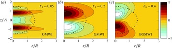
: it exhibits two successive maxima as the Froude number increases before increasing widely when it transforms into the mixed baroclinic–Gent–McWilliams instability. The structure of the mode for some selected Froude numbers is displayed in figure 19. For
 $F_{h}=0.05$
, the mode exhibits five oscillations along the vertical and is symmetric while for
 $F_{h}=0.2$
, it has only two oscillations occupying the whole pancake vortex and is anti-symmetric as seen before (see figure 7
a). This change of structure explains why there is a slight frequency jump in figure 18(b) (dashed line with triangles) and two growth rate maxima (figure 18
a). For
 $F_{h}=0.4$
(figure 19
c), the mode is of mixed type: baroclinic–Gent–McWilliams with a frequency above the cutoff
 ${\it\omega}_{r}=0.135{\it\Omega}_{0}$
of the Gent–McWilliams instability and slightly below the frequency
 ${\it\omega}_{r}=0.25{\it\Omega}_{0}$
of the baroclinic instability (figure 18
b).
(a) Maximum growth rates and (b) corresponding frequencies as a function of the Froude number
 $F_{h}$
for
 ${\it\alpha}=0.5$
,
 $Ro=1.25$
and
 $Re=10\,000$
of the different instabilities: displacement mode (


 $m=1$
; shear instability (


 $m=2$
(


Real part of the radial velocity perturbation Re(
 $u_{r}$
) of the most unstable mode for different Froude numbers: Gent–McWilliams instability for (a)
 $F_{h}=0.05$
and (b)
 $F_{h}=0.2$
and (c) mixed baroclinic–Gent–McWilliams instability for
 $F_{h}=0.4$
for
 $m=1,{\it\alpha}=0.5,Ro=1.25$
and
 $Re=10\,000$
. The dotted line indicates the extension of the base flow by showing the contour where
 ${\it\Omega}=0.1{\it\Omega}_{0}$
.

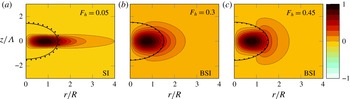
Real part of the radial velocity perturbation Re(
 $u_{r}$
) of the most unstable modes for different Froude numbers: shear instability for (a)
 $F_{h}=0.05$
and mixed baroclinic–shear instability for (b)
 $F_{h}=0.3$
and (c)
 $F_{h}=0.45$
for
 $m=2$
,
 ${\it\alpha}=0.5,Ro=1.25$
and
 $Re=10\,000$
. The dotted line indicates the extension of the base flow by showing the contour where
 ${\it\Omega}=0.1{\it\Omega}_{0}$
. The solid line (—) is the critical layer (
 $r_{c},z_{c}$
) where
 $m{\it\Omega}(r_{c},z_{c})={\it\omega}_{r}$
.

(a) Maximum growth rates and (b) corresponding frequencies as a function of aspect ratio
 ${\it\alpha}$
for
 $F_{h}=0.3$
,
 $Ro=1.25$
and
 $Re=10\,000$
of the different instabilities: displacement mode (


 $m=1$
; shear instability (


 $m=2$
(


Shear instability for
 $m=2$
(dashed line with filled circles in figure 18) is most unstable as
 $F_{h}\rightarrow 0$
and stabilizes for
 $F_{h}\simeq 0.1$
. However, it becomes unstable again for
 $F_{h}\geqslant 0.3$
but under the mixed form of a shear–baroclinic instability (dashed line with stars). When
 $F_{h}\geqslant 0.4$
, the baroclinic instability for
 $m=2$
(dashed line with crosses) becomes quickly strongly unstable as
 $F_{h}$
increases (with a growth rate higher than the upper limit of figure 18
a) but with a constant frequency
 ${\it\omega}_{r}\simeq 0.5{\it\Omega}_{0}$
. Examples of modes corresponding to these three types of instability for
 $m=2$
are shown in figure 20. For small
 $F_{h}$
, the shear instability (figure 20
a) is strongly localized near
 $z=0$
where the radial shear is maximum. In contrast, baroclinic–shear instability (figure 20
b,c) occupies the whole pancake vortex as already seen in § 3.3.
4.3 Effect of the aspect ratio
We now vary the aspect ratio keeping the other parameters to the same values as before:
 $F_{h}=0.3,Ro=1.25$
and
 $Re=10\,000$
(figure 21). For
 $m=1$
, the displacement mode (dotted line with squares) remains only marginally unstable while the growth rate of the Gent–McWilliams instability (dashed line with triangles) is large and varies non-monotonically with the aspect ratio. It exhibits two maxima, for
 ${\it\alpha}\simeq 1$
and for large
 ${\it\alpha}$
. For very small
 ${\it\alpha}$
, the growth rate rises again but the instability is then under the form of the mixed baroclinic–Gent–McWilliams instability. The full spectra for three aspect ratios are displayed in figure 22 along with the spectra for
 ${\it\alpha}=\infty$
, i.e. for a columnar vortex (solid line). For small aspect ratio (figure 22
a), there exist only two unstable modes: the displacement mode near the origin and the baroclinic–Gent–McWilliams instability near
 ${\it\omega}=0.2{\it\Omega}_{0}$
whose eigenmode is shown in figure 23(a). This markedly differs from the columnar case (solid line). In contrast, for larger aspect ratios (
 ${\it\alpha}=3$
, figure 22
b), many modes are present within the frequency range of the columnar vortex. They are however less unstable than for
 ${\it\alpha}=0.38$
. At even larger aspect ratio
 ${\it\alpha}=10$
(figure 22
c) the spectrum becomes denser with a bell shape resembling the spectra of the columnar vortex. However, the maximum growth rate for the columnar vortex is still higher. The most unstable eigenmode for
 ${\it\alpha}=10$
(figure 23
c) presents a vertical wavelength
 ${\it\lambda}\simeq 5.23R$
close to the most amplified wavelength of the columnar vortex
 ${\it\lambda}\simeq 4.5R$
. A longer typical wavelength
 ${\it\lambda}\simeq 6.16R$
is observed for
 ${\it\alpha}=3$
(figure 23
b).
Growth rate (
 ${\it\omega}_{i}/{\it\Omega}_{0}$
) and frequency (
 ${\it\omega}_{r}/{\it\Omega}_{0}$
) spectra for
 $m=1$
for different aspect ratios: (a)
 ${\it\alpha}=0.38$
, (b)
 ${\it\alpha}=3$
and (c)
 ${\it\alpha}=10$
for
 $F_{h}=0.3,Ro=1.25$
and
 $Re=10\,000$
. The solid line (——) indicates the spectrum for the columnar vortex for the same
 $F_{h},Ro$
and
 $Re$
.

Real part of the radial velocity perturbation Re(
 $u_{r}$
) of the most unstable mode for different aspect ratios: mixed baroclinic–Gent–McWilliams instability (a)
 ${\it\alpha}=0.38$
and Gent–McWilliams instability for (b)
 ${\it\alpha}=3$
and (c)
 ${\it\alpha}=10$
for
 $F_{h}=0.3,Ro=1.25$
and
 $Re=10\,000$
. The dotted line indicates the extension of the base flow by showing the contour where
 ${\it\Omega}=0.1{\it\Omega}_{0}$
.

As seen in figure 21(a), the shear instability (dashed line with filled circles) is only unstable for large aspect ratio
 ${\it\alpha}\geqslant 2$
. However, for small
 ${\it\alpha}$
, it reappears in the form of the mixed baroclinic–shear instability (dashed line with stars). The pure baroclinic instability for
 $m=2$
(dashed line with cross) also arises for very small aspect ratio.
Maximum growth rates as a function of vertical Froude number
 $F_{h}/{\it\alpha}$
for
 $Ro=1.25$
,
 $Re=10\,000$
, (a)
 $m=1$
and (b)
 $m=2$
. The upper
 $x$
axis indicates the corresponding value of
 $\sqrt{Bu}$
. The filled coloured symbols show the results when
 $F_{h}$
is varied for
 ${\it\alpha}=0.5$
, open symbols when
 ${\it\alpha}$
is varied for
 $F_{h}=0.3$
,
 $Re=10\,000$
and black filled symbols when
 ${\it\alpha}$
is varied for
 $F_{h}=0.05$
and
 $Re=360\,000$
. The shaded area indicates the gravitationally unstable region. Different symbols are used for each instability: Gent–McWilliams (


4.4 Scaling in terms of the vertical Froude number
The two previous sections have revealed different growth rate variations as a function of the Froude number
 $F_{h}$
and aspect ratio
 ${\it\alpha}$
. However, figure 24 shows that these growth rate variations are actually almost identical when represented as a function of the vertical Froude number
 $F_{h}/{\it\alpha}$
. The only deviation from this self-similarity is for small
 $F_{h}/{\it\alpha}$
: when
 $F_{h}/{\it\alpha}<0.1$
, the growth rate of the Gent–McWilliams instability grows with decreasing
 $F_{h}/{\it\alpha}$
when
 ${\it\alpha}$
is varied and
 $F_{h}$
kept constant, whereas it decreases when
 ${\it\alpha}$
is fixed and
 $F_{h}$
is varied. A small discrepancy is also observed for
 $m=2$
when
 $F_{h}/{\it\alpha}$
is small. These differences come from viscous effects due to vertical shear since they scale like
 $1/\mathscr{R}$
where
 $\mathscr{R}=ReF_{h}^{2}$
is the buoyancy Reynolds number, because the typical vertical scale
 $L_{v}$
scales like
 $L_{v}\sim F_{h}R$
. Thus, viscous effects increase when the Froude number decreases keeping the Reynolds number constant. To prove this, the results for a smaller Froude number
 $F_{h}=0.05$
but higher Reynolds number
 $Re=360\,000$
are also displayed in figure 24 (black filled symbols). This Reynolds number has been chosen so that the buoyancy Reynolds number
 $\mathscr{R}=900$
is the same as for
 $F_{h}=0.3$
and
 $Re=10\,000$
. We see that the growth rate variations are almost identical for these two parameter sets, confirming that the vertical Froude number scaling holds if the buoyancy Reynolds number is sufficiently large.
If the Rossby number is also varied but kept small, the growth rate curves for different
 $Ro$
collapse when represented as a function of
 $2F_{h}/({\it\alpha}Ro)=1/\sqrt{Bu}$
in agreement with the quasi-geostrophic theory (figure 25). We note that the transition from the Gent–McWilliams instability to the baroclinic–Gent–McWilliams instability occurs near
 $Bu\simeq 1$
as in figure 24(a) (see the upper
 $x$
axis) and in a quasi-geostrophic fluid (Nguyen et al.
Reference Nguyen, Hua, Schopp and Carton2012). However, the growth rate curves are no longer self-similar when
 $2F_{h}/({\it\alpha}Ro)$
approaches the threshold (3.2) for gravitational instability. Indeed, this threshold depends on
 $Ro$
and is thus different for
 $Ro=0.2$
and
 $Ro=0.5$
. The transition from shear instability to a baroclinic–shear instability also occurs around
 $Bu=1$
(figure 25
b).
Maximum growth rates as a function of
 $2F_{h}/({\it\alpha}Ro)$
for
 $Ro=0.5$
(open symbols) and
 $Ro=0.2$
(filled symbols) for
 $F_{h}=0.3$
,
 $Re=10\,000$
(a)
 $m=1$
and (b)
 $m=2$
. The upper
 $x$
axis indicates the corresponding value of
 $\sqrt{Bu}$
. Different symbols are used for each instability: Gent–McWilliams (


 $Ro=0.5$
and
 $Ro=0.2$
, respectively.

5 Energy budget
The previous section has evidenced a transformation of both shear and Gent–McWilliams instabilities into mixed baroclinic instabilities when the vertical Froude number is above a threshold. This transformation is apparent from the frequency and the structure of the modes. In order to confirm these transformations from the point of view of the energetics, we have computed the energy budget of the modes. To do so, the linearized equations (2.8)–(2.11) have been multiplied by the complex conjugate (
 $u_{r}^{\ast },u_{{\it\theta}}^{\ast },u_{z}^{\ast },{\it\rho}^{\ast }$
), respectively, and their real part have been integrated over the flow domain. This gives the energy balances:
 $$\begin{eqnarray}\displaystyle & \displaystyle {\it\omega}_{i}E_{k}-S_{k}=-B-D_{k}, & \displaystyle\end{eqnarray}$$
 $$\begin{eqnarray}\displaystyle & \displaystyle {\it\omega}_{i}E_{p}-S_{p}=B-D_{p}, & \displaystyle\end{eqnarray}$$
where
 $$\begin{eqnarray}\displaystyle & \displaystyle E_{k}=\int _{-Z_{\mathit{max}}}^{Z_{\mathit{max}}}\int _{0}^{R_{\mathit{max}}}\frac{1}{2}(u_{r}u_{r}^{\ast }+u_{{\it\theta}}u_{{\it\theta}}^{\ast }+u_{z}u_{z}^{\ast })r\,\text{d}r\,\text{d}z, & \displaystyle\end{eqnarray}$$
 $$\begin{eqnarray}\displaystyle & \displaystyle E_{p}=\int _{-Z_{\mathit{max}}}^{Z_{\mathit{max}}}\int _{0}^{R_{\mathit{max}}}\frac{{\it\rho}{\it\rho}^{\ast }}{2N^{2}}r\,\text{d}r\,\text{d}z, & \displaystyle\end{eqnarray}$$
 $$\begin{eqnarray}\displaystyle & \displaystyle S_{k}=-\frac{1}{4}\int _{-Z_{\mathit{max}}}^{Z_{\mathit{max}}}\int _{0}^{R_{\mathit{max}}}r\frac{\partial {\it\Omega}}{\partial r}\left(u_{r}^{\ast }u_{{\it\theta}}+u_{{\it\theta}}^{\ast }u_{r}\right)+r\frac{\partial {\it\Omega}}{\partial z}(u_{z}^{\ast }u_{{\it\theta}}+u_{z}u_{{\it\theta}}^{\ast })\,\text{d}r\,\text{d}z, & \displaystyle\end{eqnarray}$$
 $$\begin{eqnarray}\displaystyle & \hspace{-14.22636pt}\displaystyle S_{p}=-\frac{1}{4}\int _{-Z_{\mathit{max}}}^{Z_{\mathit{max}}}\int _{0}^{R_{\mathit{max}}}\left(\frac{g}{{\it\rho}_{0}N^{2}}\frac{\partial {\it\rho}_{b}}{\partial r}(u_{r}^{\ast }{\it\rho}+{\it\rho}^{\ast }u_{r})+\frac{g}{{\it\rho}_{0}N^{2}}\frac{\partial {\it\rho}_{b}}{\partial z}(u_{z}^{\ast }{\it\rho}+{\it\rho}^{\ast }u_{z})\right)\!r\,\text{d}r\,\text{d}z, & \displaystyle\end{eqnarray}$$
 $$\begin{eqnarray}\displaystyle & \displaystyle B=\frac{1}{4}\int _{-Z_{\mathit{max}}}^{Z_{\mathit{max}}}\int _{0}^{R_{\mathit{max}}}({\it\rho}u_{z}^{\ast }+{\it\rho}^{\ast }u_{z})r\,\text{d}r\,\text{d}z. & \displaystyle\end{eqnarray}$$
 $E_{k}$
and
 $E_{p}$
are the kinetic and potential energies of the perturbation. The term
 $S_{k}$
(
 $S_{p}$
) represents the transfer of kinetic (potential) energy from the base flow to the perturbation. The term
 $B$
is the energy conversion from the kinetic to potential energy of the perturbation.
 $D_{k}$
and
 $D_{p}$
are the kinetic and potential energy dissipations. They are small and will not be discussed here. The transfers are plotted in figure 26 as a function of
 $F_{h}/{\it\alpha}$
for
 $m=1$
(figure 26
a) and
 $m=2$
(figure 26
b) for
 $Ro=1.25$
and
 $Re=10\,000$
. These parameters correspond to the coloured filled/open symbols in figure 24. For both
 $m=1$
and
 $m=2$
, the kinetic energy transfer
 $S_{k}$
is positive for
 $F_{h}/{\it\alpha}<0.5$
(corresponding to
 $Bu>1.5$
), while the potential energy transfer
 $S_{p}$
is smaller and negative. This means that the source of the instability is the kinetic energy of the base flow as for the instabilities of a columnar vortex (
 ${\it\alpha}=\infty$
). A part of the kinetic energy of the perturbation is converted to potential energy since the energy conversion
 $B$
is positive except for
 $m=2$
for
 $F_{h}/{\it\alpha}<0.1$
when
 $F_{h}>0.5$
(figure 26
b). In contrast, when
 $F_{h}/{\it\alpha}>0.5~(Bu<1.5)$
, the potential energy transfer
 $S_{p}$
becomes positive while
 $S_{k}$
is negative. The energy source of the instability is therefore the potential energy of the base flow.
Kinetic and potential energy transfers
 $S_{k}$
(

 $S_{p}$
(

 $B$
(

 $F_{h}/{\it\alpha}$
for (a)
 $m=1$
and (b)
 $m=2$
for
 $Ro=1.25$
and
 $Re=10\,000$
. The filled symbols indicate when
 $F_{h}$
is varied for
 ${\it\alpha}=0.5$
and open symbols when
 ${\it\alpha}$
is varied for
 $F_{h}=0.3$
.

Figure 27 shows that a similar transition occurs when
 $Ro$
is varied while
 $F_{h}$
and
 ${\it\alpha}$
are kept constant. The transfers for
 $m=1$
(figure 27
a) correspond to those of the Gent–McWilliams and baroclinic–Gent–McWilliams instabilities shown in figure 10. As
 $Ro$
decreases, the source of the energy perturbation changes from kinetic to potential around
 $Ro\simeq 2{-}3$
when the Gent–McWilliams instability transforms into the mixed baroclinic–Gent–McWilliams instability. The same happens for
 $m=2$
(figure 27
b) around
 $Ro\simeq 1$
when shear instability changes into a baroclinic–shear instability (see figure 15). This confirms that the baroclinicity plays an important role for large
 $F_{h}/{\it\alpha}$
or small
 $Ro$
and the instabilities are then of mixed nature: baroclinic–Gent–McWilliams and baroclinic–shear instabilities.
Kinetic and potential energy transfers
 $S_{k}$
(

 $S_{p}$
(

 $B$
(

 $Ro$
for (a)
 $m=1$
,
 ${\it\alpha}=0.5$
and for (b)
 $m=2$
,
 ${\it\alpha}=1.2$
for
 $F_{h}=0.5$
and
 $Re=10\,000$
. The plot (a) corresponds to the Gent–McWilliams, baroclinic–Gent–McWilliams and baroclinic instabilities shown in figure 10. The plot (b) corresponds to the shear and baroclinic–shear instabilities shown in figure 15.

6 Condition of existence of shear instability
In this section, we will show that the variations of the growth rate of shear instability for
 $m=2$
as a function of
 $Ro$
,
 $F_{h}$
and
 ${\it\alpha}$
can be directly understood from the characteristics of the shear instability for a columnar vortex. As demonstrated in part 1 for stratified non-rotating fluids, the shear instability for columnar vortices only exists for vertical wavenumbers
 $k$
in the range
 $kRF_{h}<1.6$
. The minimum vertical wavelength is therefore
 ${\it\lambda}_{\mathit{min}}\simeq 4F_{h}R$
. One wavelength will fit in the thickness of the pancake vortex
 $2{\it\alpha}R$
only if
 $F_{h}/{\it\alpha}<0.5$
. This condition turns out to explain very well the existence of the shear instability for pancake vortices in stratified non-rotating fluids. Here, we extend this criterion to arbitrary Rossby number
 $Ro$
.
Figure 28(a) shows the growth rate of shear instability for a columnar vortex for
 $Ro=2$
as a function of the rescaled vertical wavenumber
 $kRF_{h}$
. The growth rate is maximum in the two-dimensional limit
 $k=0$
and decreases monotonically as
 $kRF_{h}$
increases. When
 $F_{h}$
is varied between 0.1 and 2 with
 $Ro$
fixed, all the curves remain similar and stabilize for
 $kRF_{h}\simeq 0.6$
. This illustrates the fact that the growth rate depends only on
 $kRF_{h}$
for small
 $F_{h}$
for any given
 $Ro$
. The growth rate of shear instability is shown in figure 28(b) as a function of
 $Ro$
and
 $kRF_{h}$
. The wavenumber cutoff
 $kRF_{h}$
first increases as
 $Ro$
decreases from
 $Ro=\infty$
and then decreases and follows the quasi-geostrophic scaling law
 $kRF_{h}/Ro=\text{const.}$
for small Rossby numbers. For negative Rossby numbers, the cutoff again increases monotonically as
 $Ro$
decreases. This shows that the wavenumber cutoff can be written
 $kF_{h}R=c(Ro)$
, where
 $c$
is a function of
 $Ro$
. A similar evolution of the cutoff of shear instability is observed for parallel horizontal flows sheared horizontally in strongly stratified-rotating fluids. In particular, in the case of the hyperbolic tangent (
 $\tanh$
) profile, Blumen (Reference Blumen1971) has obtained an analytical expression for the neutral wavenumbers:
 $(F_{h}k_{z})^{2}(1-1/Ro)^{2}+k_{x}^{2}=1$
, where
 $k_{x}$
and
 $k_{z}$
are the streamwise and vertical (spanwise) wavenumbers, respectively. In the present case, we did not find an exact expression for the cutoff vertical wavenumber but, guided by the expression of Blumen (Reference Blumen1971), we have found that
 $c(Ro)$
can be well approximated by
 $$\begin{eqnarray}c(Ro)=\frac{1}{\sqrt{c_{1}+{\displaystyle \frac{c_{2}}{Ro}}+{\displaystyle \frac{c_{3}}{Ro^{2}}}}},\end{eqnarray}$$
where
 $c_{1}=0.44$
,
 $c_{2}=-4.8$
and
 $c_{3}=18.2$
are empirical constants. The rescaled cutoff vertical wavenumber
 $kRF_{h}$
obtained from (6.1) is shown by a dashed line in figure 28(b). The minimum vertical wavelength of the shear instability for a columnar vortex in a strongly stratified fluid for an arbitrary Rossby number is therefore
 ${\it\lambda}_{\mathit{min}}=2{\rm\pi}F_{h}R/c(Ro)$
. Hence, one wavelength will fit within the thickness of the pancake vortex if
 ${\it\lambda}_{\mathit{min}}\leqslant 2{\it\alpha}R$
, i.e. if
 $F_{h}/{\it\alpha}\leqslant c(Ro)/{\rm\pi}$
.
Growth rate of the shear instability for
 $m=2$
for a columnar vortex as a function of the rescaled axial wavenumber
 $kRF_{h}$
: (a) for different Froude numbers
 $F_{h}$
:

 $F_{h}=0.1$
;

 $F_{h}=0.5$
;

 $F_{h}=1$
;

 $F_{h}=2$
, for
 $Ro=2$
and
 $Re=10\,000$
. (b) Growth rate
 ${\it\omega}_{i}/{\it\Omega}_{0}$
contours of shear instability for a columnar vortex as a function of the Rossby number
 $Ro$
and the rescaled vertical wavenumber
 $kRF_{h}$
for
 $F_{h}=0.2$
and
 $Re=10\,000$
. The vertical dotted line is the wavenumber cutoff
 $kRF_{h}=1.6$
for
 $Ro=\infty$
. The dashed line in (b) shows the approximation (6.1) of the rescaled cutoff vertical wavenumber.

Assuming further that the equivalent vertical wavenumber of the most unstable mode of shear instability for the pancake vortex is always the smallest fitting along the vertical, i.e.
 $kR={\rm\pi}/{\it\alpha}$
, one can compare the growth rate of the shear instability for columnar and pancake vortices as done in figure 29 for two different Rossby numbers
 $Ro=1.25$
and
 $Ro=-5$
. For both
 $Ro$
, the growth rate for columnar and pancake vortices are in good agreement and vanish around the same value of
 $F_{h}/{\it\alpha}$
(or equivalently
 $kRF_{h}/{\rm\pi}$
). For
 $Ro=1.25$
, the growth rate for the pancake vortex rises again for
 $F_{h}/{\it\alpha}>0.5$
owing to the mixed baroclinic–shear instability.
Maximum growth rate of shear instability for columnar (for
 $kR={\rm\pi}/{\it\alpha}$
) (


 $F_{h}/{\it\alpha}$
for
 $m=2,F_{h}=0.3$
and
 $Re=10\,000$
for (a)
 $Ro=1.25$
and (b)
 $Ro=-5$
. The shaded region is the gravitationally unstable region. The line


Maximum growth rate of shear instability for columnar (for
 $kR={\rm\pi}/{\it\alpha}$
) (

 ${\it\alpha}=1.2$
) (

 $Ro$
for
 $m=2$
,
 $F_{h}=0.5$
and
 $Re=10\,000$
. The shaded region is the gravitationally unstable region. The line


A similar comparison is made in figure 30 but now as a function of the Rossby number for the parameters
 ${\it\alpha}=1.2,F_{h}=0.5$
and
 $Re=10\,000$
that have been presented in § 3.3. The maximum growth rate of the shear instability for the pancake vortex agrees quite well with the one of the columnar vortex for the vertical wavenumber
 $kR={\rm\pi}/{\it\alpha}$
. In particular, the shear instability is stabilized in the same range of Rossby number:
 $-22\lesssim Ro\lesssim 3$
. Again, the growth rate for the pancake vortex rises for small Rossby number but under the mixed form of the baroclinic–shear instability.
As a conclusion, these results demonstrate that the maximum growth rate of the shear instability in pancake vortices corresponds in good approximation to its growth rate in columnar vortices for the smallest vertical wavenumber
 $kR={\rm\pi}/{\it\alpha}$
fitting in the pancake vortex. When this wavenumber is beyond the upper wavenumber cutoff, i.e.
 ${\rm\pi}/{\it\alpha}>c(Ro)/F_{h}$
, the shear instability is suppressed in pancake vortices.
7 Scaling laws for the Gent–McWilliams instability
The fluctuations of the growth rate of the Gent–McWilliams instability as a function of the vertical Froude number
 $F_{h}/{\it\alpha}$
(figure 24
a) can be also understood by comparison to the columnar case. First, the equivalent vertical wavenumber
 $k$
of the Gent–McWilliams instability for pancake vortices can be estimated as
 $k=2{\rm\pi}/{\it\lambda}$
where
 ${\it\lambda}$
is twice the vertical distance between contiguous minimum and maximum of the radial velocity perturbation. The growth rate is plotted as a function of this wavenumber scaled by
 $F_{h}R$
in figure 31 (symbols). The corresponding growth rate for a columnar vortex is shown by the grey continuous line.
Maximum growth rate of the Gent–McWilliams instability (
 $m=1$
) as a function of the estimated vertical wavenumber
 $kRF_{h}$
for
 $Ro=1.25$
and
 $Re=10\,000$
. (a)
 ${\it\alpha}$
is varied for
 $F_{h}=0.3$
and (b)
 $F_{h}$
is varied for
 ${\it\alpha}=0.5$
. The thick grey line corresponds to the growth rate of the columnar vortex for the same parameters. Two different symbols are used depending on
 $F_{h}/{\it\alpha}$
:

 $F_{h}/{\it\alpha}>0.1$
and

 $F_{h}/{\it\alpha}<0.1$
. Open diamond symbols (

 $\mathscr{R}=F_{h}^{2}Re=25$
when
 $F_{h}$
is varied for
 ${\it\alpha}=0.5$
.

Let us first focus on figure 31(a) where the Froude number is fixed to
 $F_{h}=0.3$
while the aspect ratio varies. When
 ${\it\alpha}$
increases from
 ${\it\alpha}=0.5$
to
 ${\it\alpha}=3$
, the growth rate of the Gent–McWilliams instability for the pancake vortex (dotted line with triangles) increases and then decreases in a similar fashion as the columnar case. In particular, the growth rate is maximum for
 $kRF_{h}=0.6$
near the most amplified wavenumber
 $kRF_{h}$
of the columnar vortex. Nevertheless, the growth rate maximum for the pancake vortex is much smaller than for the columnar vortex. Along the curve, the eigenmodes remain similar to the one shown in figure 19(b), i.e. the mode has a single oscillation along the vertical and occupies the whole pancake vortex. However, when
 ${\it\alpha}=3$
, a secondary mode with several oscillations along the vertical (see figure 23
b) starts to have a growth rate as high as the primary mode. The wavenumber of this secondary mode is much higher and its growth rate is shown by the dashed line with diamonds in figure 31(a). When
 ${\it\alpha}$
is further increased, the growth rate of this secondary mode increases rapidly but its estimated wavenumber decreases only slightly toward the most amplified wavenumber of the columnar vortex. Along this curve, the eigenmode has therefore more and more oscillations along the vertical like in figure 23(c). In other words, the confinement effect due to the pancake shape becomes weaker as the vortex becomes taller.
Alternatively, when
 ${\it\alpha}$
is kept constant at
 ${\it\alpha}=0.5$
(figure 31
b) a similar evolution is first observed when the Froude number is decreased from
 $F_{h}=0.3$
to
 $F_{h}=0.05$
(dashed line with triangles). When
 $F_{h}=0.05$
, a secondary mode (dashed line with diamonds) becomes as unstable as the primary mode. This occurs for the same vertical Froude number
 $F_{h}/{\it\alpha}=0.1$
as in figure 31(a). The structure of this secondary mode can be seen in figure 19(a). However, the growth rate of the secondary mode first increases slightly as
 $F_{h}$
is further decreased and then it decreases toward zero while its wavenumber also decreases. The difference in behaviour compared to figure 31(a) comes from the fact that the buoyancy Reynolds number
 $\mathscr{R}=ReF_{h}^{2}$
becomes too low when the Froude number
 $F_{h}$
is decreased below
 $0.05$
. Indeed, if the Reynolds number is increased at the same time as
 $F_{h}$
is decreased, so as to keep the buoyancy Reynolds number constant
 $\mathscr{R}=25$
, the growth rate (open diamonds in figure 31
b) rises toward the growth rate peak for the columnar vortex as
 $F_{h}$
decreases as in figure 31(a).
8 Detailed study of baroclinic instability
In §§ 3 and 4, the baroclinic instability has been observed for
 $m=1$
and
 $m=2$
near the threshold for gravitational instability. Here, we will further study its dependence on the Rossby number
 $Ro$
and the vertical Froude number
 $F_{h}/{\it\alpha}$
. In addition, we will show that baroclinic instability destabilizes also higher azimuthal wavenumbers. A theoretical criterion and scaling laws for baroclinic instability will be next derived following the approach used in part 1 for stratified non-rotating fluids.
8.1 A typical example
Figure 32 shows the spectra for
 ${\it\alpha}=0.5,F_{h}=0.3,Ro=0.4$
and
 $Re=10\,000$
for different azimuthal wavenumbers
 $m$
. These control parameters are just below the threshold of gravitational instability which is
 $F_{h}=0.32$
for
 ${\it\alpha}=0.5$
and
 $Ro=0.4$
. Among all azimuthal wavenumbers,
 $m=2$
is the most unstable. For each
 $m$
, the most unstable mode is anti-symmetric (black symbol) and the second most unstable mode is symmetric (grey symbol). Nevertheless, the growth rate difference between anti-symmetric and symmetric modes becomes very small as
 $m$
increases. We will show that these modes are due to baroclinic instability. However, the displacement mode is also observed for
 $m=1$
near the origin and the baroclinic–shear instability for
 $m=2$
is located near
 ${\it\omega}_{r}/{\it\Omega}_{0}=0.18$
with a small growth rate. Note also that the leading mode for
 $m=1$
is the baroclinic–Gent–McWilliams instability which derives continuously from the Gent–McWilliams instability. For higher azimuthal wavenumbers,
 $m\geqslant 3$
, only the baroclinic instability exists. No instability has been found for
 $m=0$
and
 $m\geqslant 6$
. The characteristic frequency of each azimuthal wavenumber is proportional to
 $m$
:
 ${\it\omega}_{r}/{\it\Omega}_{0}\simeq 0.25m$
, i.e. the azimuthal phase velocity is constant. In fact, this corresponds to the angular velocity of the base flow
 ${\it\Omega}(r_{b},z_{b})\simeq 0.25$
at the point
 $r_{b}=0,z_{b}=1.17{\it\Lambda}$
where the vertical density gradient
 $\partial {\it\rho}_{t}/\partial z$
is maximum for
 ${\it\alpha}=0.5,F_{h}=0.3$
and
 $Ro=0.4$
.
Growth rate (
 ${\it\omega}_{i}/{\it\Omega}_{0}$
) and frequency (
 ${\it\omega}_{r}/{\it\Omega}_{0}$
) spectra for different azimuthal wavenumbers:
 $m=1$
(

 $m=2$
(

 $m=3$
(

 $m=4$
(

 $m=5$
(

 ${\it\alpha}=0.5$
,
 $F_{h}=0.3,Ro=0.4$
, and
 $Re=10\,000$
. Grey and black symbols indicate symmetric and anti-symmetric modes, respectively.

Figure 33 shows the first three anti-symmetric eigenmodes for
 $m=3$
. As already shown for
 $m=1$
(figure 9), the number of oscillations in the radial direction increases with the mode number while the vertical structure remains the same. Figure 34(a) shows the growth rate as a function of the radial wavenumber
 $l=2{\rm\pi}/{\it\lambda}_{r}$
where the radial wavelength
 ${\it\lambda}_{r}$
is estimated as twice the distance between two successive extrema, as illustrated in figure 33(b). For each azimuthal wavenumber, the growth rate decreases monotonically as
 $l$
increases. As already visible in figure 32, the maximum growth rate exhibits a bell-shaped curve as a function of
 $m$
(figure 34
b). These wavenumber properties are very reminiscent of baroclinic instability in parallel shear flows (Vallis Reference Vallis2006).
Real part of the radial velocity perturbation Re
 $(u_{r})$
for the first three anti-symmetric baroclinic eigenmodes for
 $m=3$
: (a)
 $(3,1)$
, (b)
 $(3,3)$
and (c)
 $(3,5)$
for
 ${\it\alpha}=0.5$
,
 $F_{h}=0.3$
,
 $Ro=0.4$
and
 $Re=10\,000$
. The dotted line indicates the extension of the base flow by showing the contour where
 ${\it\Omega}=0.1{\it\Omega}_{0}$
. The double dotted dashed line (

(a) Growth rate (
 ${\it\omega}_{i}/{\it\Omega}_{0}$
) as a function of the radial wavenumber
 $l$
for different azimuthal wavenumbers:
 $m=1$
(

 $m=2$
(

 $m=3$
(

 $m=4$
(

 $m=5$
(

 $m$
for
 ${\it\alpha}=0.5$
,
 $F_{h}=0.3,Ro=0.4,$
and
 $Re=10\,000$
.

8.2 Parametric study
Figure 35 outlines the effect of the Rossby number on the maximum growth rate and corresponding frequency of the baroclinic instability for each azimuthal wavenumber for
 ${\it\alpha}=0.5,F_{h}=0.3$
and
 $Re=10\,000$
. When
 $Ro$
increases, the growth rate decreases faster as
 $m$
increases. Hence,
 $m=3$
is the most unstable azimuthal wavenumber when
 $Ro$
is close to the threshold for the gravitational instability whereas
 $m=1$
becomes the most unstable for
 $Ro\geqslant 0.5$
. In between,
 $m=2$
is the most unstable. In contrast, the frequency of each azimuthal wavenumber is independent of the Rossby number (figure 35
b). Similarly, figure 36 shows the effect of the Froude number for
 ${\it\alpha}=0.5,Ro=0.4$
and
 $Re=10\,000$
. The frequency is again independent of the Froude number (figure 36
b) whereas the maximum growth rate (figure 36
a) increases with
 $F_{h}/{\it\alpha}$
at a rate increasing with
 $m$
.
(a) Maximum growth rate and (b) corresponding frequency of the baroclinic instability (dark solid lines) as a function of
 $Ro$
for different azimuthal wavenumbers:
 $m=1$
(

 $m=2$
(

 $m=3$
(

 $m=4$
(

 $m=5$
(

 ${\it\alpha}=0.5,F_{h}=0.3$
and
 $Re=10\,000$
. The shaded area indicates the gravitationally unstable region.

(a) Maximum growth rate and (b) corresponding frequency of the baroclinic instability (dark solid lines) as a function of
 $F_{h}/{\it\alpha}$
for different azimuthal wavenumbers:
 $m=1$
(

 $m=2$
(

 $m=3$
(

 $m=4$
(

 $m=5$
(

 ${\it\alpha}=0.5,Ro=0.4,$
and
 $Re=10\,000$
. The shaded area indicates the gravitationally unstable region.

8.3 A simple analytical model
In part 1, a model consisting of a bounded vortex with an angular velocity varying only in the vertical direction has been considered and shown to account qualitatively for the characteristics of baroclinic instability in stratified non-rotating fluids. Such a model takes into account the main features of the base flow in the core of the pancake vortex where the baroclinic instability develops. Its stability can be solved analytically when the vertical variations are weak. Here, this model is extended to take into account a background rotation. The base angular velocity of the vortex is assumed to be
 $$\begin{eqnarray}{\it\Omega}=\tilde{{\it\Omega}}_{0}-\tilde{{\it\Omega}}_{1}z,\end{eqnarray}$$
where
 $\tilde{{\it\Omega}}_{0}$
and
 $\tilde{{\it\Omega}}_{1}$
are constants. From the thermal wind relation (2.4), the base density is obtained as
 $$\begin{eqnarray}{\it\rho}_{b}=\frac{{\it\rho}_{0}}{g}\left[\tilde{{\it\Omega}}_{0}+\frac{f}{2}-\tilde{{\it\Omega}}_{1}z\right]\tilde{{\it\Omega}}_{1}r^{2}.\end{eqnarray}$$
As in part 1, we consider that the base flow is contained in a rigid cylinder of radius
 $R$
and height
 $H$
between
 $z=-H/2$
and
 $z=H/2$
. By assuming that the vertical variations are weak, i.e.
 $\tilde{{\it\Omega}}_{1}H\ll |\tilde{{\it\Omega}}_{0}+f/2|$
, the equations (2.8)–(2.12) in the inviscid limit can be reduced at leading order in
 $\tilde{{\it\Omega}}_{1}$
to
 $$\begin{eqnarray}\frac{1}{r}\frac{\partial }{\partial r}\left(r\frac{\partial p}{\partial r}\right)-\left[\frac{m^{2}}{r^{2}}+C^{2}\frac{\partial ^{2}}{\partial z^{2}}\right]p=0+O(\tilde{{\it\Omega}}_{1}^{2}),\end{eqnarray}$$
where
 $C=2|\tilde{{\it\Omega}}_{0}+f/2|/N$
. Note that the hypothesis
 $\tilde{{\it\Omega}}_{1}H\ll |\tilde{{\it\Omega}}_{0}+f/2|$
is not valid around
 $\tilde{Ro}\equiv 2\tilde{{\it\Omega}}_{0}/f=-1$
. Here, the dimensionless numbers are denoted with a tilde in order to distinguish them from the ones defined in (2.13). The Coriolis parameter
 $f$
enters the problem only through the constant
 $C$
in (8.3). The general solution of (8.3) is
 $$\begin{eqnarray}p=\text{J}_{m}(Ckr)\left(A\cosh kz+B\sinh kz\right),\end{eqnarray}$$
where
 $\text{J}_{m}$
is the Bessel function of order
 $m$
of the first kind and
 $A$
and
 $B$
are constants. Imposing the boundary conditions
 $u_{z}(z=\pm H/2)=0$
and
 $u_{r}(r=R)=0$
yields two relations similar to those for the classical Eady problem (Vallis Reference Vallis2006)
 $$\begin{eqnarray}\displaystyle & \displaystyle {\it\omega}=m\tilde{{\it\Omega}}_{0}+\frac{m\tilde{{\it\Omega}}_{1}}{k}\sqrt{\left(1-\frac{kH}{2\tanh (kH/2)}\right)\left(1-\frac{kH\tanh (kH/2)}{2}\right)}, & \displaystyle\end{eqnarray}$$
 $$\begin{eqnarray}\displaystyle & \displaystyle CkR={\it\mu}_{m,n}, & \displaystyle\end{eqnarray}$$
where
 ${\it\mu}_{m,n}$
is the
 $n$
th root of J
 $_{m}$
. Combining the condition for instability
 $kH<2.4$
and the fact that
 ${\it\mu}_{m,n}>{\it\mu}_{1,1}=3.83$
, yields the instability condition
 $$\begin{eqnarray}\frac{\tilde{F_{h}}}{\tilde{{\it\alpha}}}\left|1+\frac{1}{\tilde{Ro}}\right|>0.8,\end{eqnarray}$$
where
 $\tilde{{\it\alpha}}=H/R$
and
 $\tilde{F_{h}}=\tilde{{\it\Omega}}_{0}/N$
. This condition simply states that the Burger number
 $\tilde{Bu}=\tilde{{\it\alpha}}^{2}N^{2}/(f+2\tilde{{\it\Omega}}_{0})^{2}$
based on the absolute angular velocity
 $\tilde{{\it\Omega}}_{0}+f/2$
should be below a threshold
 $\tilde{Bu}<0.4$
for instability. When
 $\tilde{Ro}\ll 1$
, equation (8.7) recovers the classical condition for baroclinic instability (Eady Reference Eady1949; Saunders Reference Saunders1973; Hide & Mason Reference Hide and Mason1975). We can also derive scaling laws for the maximum growth rate and the most amplified wavenumber (8.5). For any
 $m$
, the growth rate is maximum for the first root of the Bessel function
 $n=1$
. An asymptotic expansion of this root for large
 $m$
is
 ${\it\mu}_{m,1}=m+1.856m^{1/3}+O(m^{-1/3})$
(Abramowitz & Stegun Reference Abramowitz and Stegun1972). Taking only the leading order of this expansion, i.e.
 ${\it\mu}_{m,1}\sim m$
, (8.6) implies
 $m/k=CR$
. The growth rate is thus maximum when the term inside the square root in (8.5) is minimum, i.e. when
 $kH=1.6$
. The most amplified azimuthal wavenumber is therefore
 $$\begin{eqnarray}m_{\mathit{max}}\simeq 3.2\frac{\tilde{F_{h}}}{\tilde{{\it\alpha}}}\left|1+\frac{1}{\tilde{Ro}}\right|,\end{eqnarray}$$
and the maximum growth rate is
 $$\begin{eqnarray}{\it\omega}_{imax}\simeq 0.6\tilde{{\it\Omega}}_{1}R\frac{\tilde{F_{h}}}{\tilde{{\it\alpha}}}\left|1+\frac{1}{\tilde{Ro}}\right|,\end{eqnarray}$$
for large
 $m$
. These scaling laws are tested in figure 37 for baroclinic instability of the pancake vortex by assuming that
 $F_{h}/{\it\alpha}|1+1/Ro|$
is equivalent to
 $\tilde{F_{h}}/\tilde{{\it\alpha}}|1+1/\tilde{Ro}|$
. Different combinations of
 $F_{h}$
and
 $Ro$
are shown for
 ${\it\alpha}=0.5$
and
 $Re=10\,000$
. As seen in figure 37(a), the maximum growth rates align along a straight line when represented as a function of
 $F_{h}/{\it\alpha}|1+1/Ro|$
. Baroclinic instability only occurs for
 $F_{h}/{\it\alpha}|1+1/Ro|\geqslant 1.46$
in qualitative agreement with (8.7). Note that the leftmost point (star) in figure 37(a), which is slightly away from the other points, is for a negative Rossby number
 $Ro=-5$
. Similarly, figure 37(b) shows that the most amplified azimuthal wavenumber increases approximately linearly with
 $F_{h}/{\it\alpha}|1+1/Ro|$
in agreement with (8.8).
(a) Maximum growth rate and (b) most amplified azimuthal wavenumber
 $m$
of the baroclinic instability for different combinations of
 $Ro$
and
 $F_{h}$
:
 $Ro=0.4$
,
 $F_{h}$
varies

 $F_{h}=0.3$
,
 $Ro$
varies

 $Ro=1$
,
 $F_{h}=0.42$

 $Ro=5$
,
 $F_{h}=0.67$

 $Ro=10$
,
 $F_{h}=0.7$

 $Ro=-5$
,
 $F_{h}=0.8$

 $Ro=\infty$
,
 $F_{h}$
varies

 ${\it\alpha}=0.5$
,
 $Re=10\,000$
. The dotted line in (a) is a fit.

Figure 38 displays a map of the domain of existence of the baroclinic instability in the parameter space (
 $F_{h}/{\it\alpha}$
,
 $Ro$
). The dashed line represents the threshold
 $F_{h}/{\it\alpha}|1+1/Ro|=1.46$
deduced from figure 37(a). The shaded region is gravitationally unstable. The circle symbols indicate the parameters for which the baroclinic instability has been observed for
 $m=2$
,
 $Re=10\,000$
and
 ${\it\alpha}=0.5$
while the cross symbols correspond to the parameters stable to the baroclinic instability for
 $m=2$
. We can see that there is a good agreement between the threshold
 $F_{h}/{\it\alpha}|1+1/Ro|=1.46$
and the numerical results for positive Rossby number. However, the threshold departs from the numerical results for negative Rossby numbers around
 $Ro\simeq -5$
. This is most likely due to the assumption of slow vertical variation
 $\tilde{{\it\Omega}}_{1}H\ll \tilde{{\it\Omega}}_{0}+f/2$
used to derive the theoretical scaling laws. This hypothesis indeed breaks down around
 $\tilde{Ro}=-1$
and this may affect a large range of negative Rossby numbers
 $Ro$
. Furthermore, the location where the density gradient is maximum actually varies with the Rossby number, implying that
 $\tilde{{\it\Omega}}_{0}$
also varies with
 $Ro$
. These variations could be taken into account in a refined analysis.
Domain of existence of the baroclinic instability for
 $m=2$
as a function of
 $F_{h}/{\it\alpha}$
and
 $Ro$
for
 ${\it\alpha}=0.5$
and
 $Re=10\,000$
: circles (

 $\times$
) are for the stable case. The shaded area indicates the region unstable to gravitational instability and the dashed line (– – –) corresponds to the threshold
 $F_{h}/{\it\alpha}|1+1/Ro|=1.46$
.

Domains of existence of the different instabilities for the azimuthal wavenumbers (a,b)
 $m=0$
, (c,d)
 $m=1$
and (e,f)
 $m=2$
as a function of
 $Ro$
and
 $F_{h}/{\it\alpha}$
(a,c,e) and
 $Bu=Ro^{2}{\it\alpha}^{2}/(4F_{h}^{2})$
(b,d,f) for
 $Re=10\,000$
and various aspect ratio
 ${\it\alpha}$
. The symbols indicate the different instabilities for each set of parameters investigated: in (a–f): centrifugal (CI)


 $\times$
). In (c,d): Gent–McWilliams (GMWI) ▴; baroclinic–Gent–McWilliams (BGMWI)
 $+$
. In (e,f): shear (SI) ▴ and baroclinic–shear (BSI)
 $+$
instabilities. In the white region in (d), only the displacement mode (DM) is unstable for finite
 $Re$
. The shaded area indicates the gravitationally unstable region (GI), the thick solid line shows the threshold for centrifugal instability for
 ${\it\alpha}=0.5$
derived from (3.5), the dotted line is the threshold
 $F_{h}/{\it\alpha}<c(Ro)/{\rm\pi}$
for shear instability and the dashed line is the threshold for baroclinic instability:
 $F_{h}/{\it\alpha}|1+1/Ro|=1.46$
. The dashed dotted lines in (c,d) and (e,f) show the empirical thresholds for baroclinic–Gent–McWilliams instability (
 $Bu=0.7Ro+0.1$
) and baroclinic–shear instability (
 $Bu=1.3/(-Ro+2.26)$
for
 $|Ro|<2$
and
 $Bu=2.5Ro$
for
 $Ro>2$
) instabilities, respectively.

9 Map of the instabilities
9.1 Parameter space (
$F_{h}/{\it\alpha}$
,
$Ro$
)


Figure 39(a,c,e) summarize the different instabilities observed for each azimuthal wavenumber
 $m=0,1$
and 2 in the parameter space (
 $F_{h}/{\it\alpha}$
,
 $Ro$
) for
 $Re=10\,000$
and various aspect ratios. The symbols indicate the instability type while the lines indicate the different semi-theoretical thresholds that have been derived throughout the paper. These conditions are generally in good agreement with the numerical results for all the parameters investigated. In summary, a centrifugal instability exists for
 $m=0,1,2$
for sufficiently high Rossby and Froude numbers. The solid lines correspond to the thresholds for centrifugal instability for
 ${\it\alpha}=0.5$
that can be obtained from the asymptotic formula (3.5). This formula shows that the aspect ratio of the vortex has no effect and there is a stabilization at low Froude numbers because the buoyancy Reynolds number
 $\mathscr{R}=ReF_{h}^{2}$
, which controls viscous effects, decreases. Shear instability for
 $m=2$
is present below a critical vertical Froude number
 $F_{h}/{\it\alpha}$
depending on the Rossby number
 $F_{h}/{\it\alpha}<c(Ro)/{\rm\pi}$
, where
 $c(Ro)$
is defined in (6.1) (dotted line in figure 39
e). However, for higher
 $F_{h}/{\it\alpha}$
, it reappears under the mixed form of a baroclinic–shear instability when the Rossby number is not too large (dashed dotted line in figure 39(e)
 $Ro\lesssim 10F_{h}^{2}/{\it\alpha}^{2}$
for
 $Ro>0$
and
 $Ro\gtrsim -1.1F_{h}/{\it\alpha}$
for
 $Ro<0$
). The Gent–McWilliams instability for
 $m=1$
(triangles in figure 39
c) is observed over wide ranges of
 $Ro$
and
 $F_{h}/{\it\alpha}$
except when it transforms to the baroclinic–Gent–McWilliams instability (squares in figure 39
c) for small Rossby numbers such that
 $F_{h}/{\it\alpha}>|Ro|/(2\sqrt{0.7Ro+0.1})$
(dashed dotted lines in figure 39
c). A baroclinic instability occurs when
 $F_{h}/{\it\alpha}|1+1/Ro|>1.46$
(dashed lines in figure 39
c,e), i.e. only in a small band close to the threshold for the gravitational instability (shaded region).
9.2 Parameter space (
$Bu$
,
$Ro$
)


Figures 39(b,d,f) display the same instability maps but focused on the region
 $|Ro|<2$
which pertains to most mesoscale oceanic vortices. In addition, the
 $x$
-axis is now the Burger number
 $Bu=Ro^{2}{\it\alpha}^{2}/(4F_{h}^{2})$
instead of the vertical Froude number
 $F_{h}/{\it\alpha}$
. Indeed, the Burger number is more appropriate to describe the region of small Rossby number since it is the only non-dimensional parameter in the quasi-geostrophic limit. Only the range
 $0\leqslant Bu\leqslant 2$
is displayed as in Nguyen et al. (Reference Nguyen, Hua, Schopp and Carton2012). In these ranges, we see that centrifugal instability for
 ${\it\alpha}=0.5$
exists only in the bottom left corner for sufficiently negative
 $Ro$
and small
 $Bu$
. The Gent–McWilliams instability (triangles in figure 39
d) occurs when
 $Bu\gtrsim 1$
. In contrast, the baroclinic–Gent–McWilliams instability exists mostly for positive
 $Ro$
in a band adjacent to the domain of baroclinic instability. The threshold can be fitted approximately by
 $Bu\simeq 0.7Ro+0.1$
(dashed dotted line in figure 39
d). Hence, there is an intermediate range of Burger number where only the displacement mode is unstable for
 $m=1$
for finite Reynolds number. For
 $m=2$
(figure 39
f), the domain of existence of the baroclinic–shear instability is also contiguous to the domain unstable to baroclinic instability. The upper Burger number limit is given by
 $Bu\simeq 1.3/(-Ro+2.26)$
. Just above this threshold,
 $m=2$
perturbations are stable since shear instability starts to be active only when
 $Bu\gtrsim 7$
. These results are in general consistent with those in the quasi-geostrophic limit (
 $Ro\rightarrow 0$
) in continuously stratified fluids (Nguyen et al.
Reference Nguyen, Hua, Schopp and Carton2012) or in two-layer fluids (Ikeda Reference Ikeda1981; Flierl Reference Flierl1988; Helfrich & Send Reference Helfrich and Send1988; Benilov Reference Benilov2003). In particular, Flierl (Reference Flierl1988) reports for piecewise profiles that the
 $m=1$
mode is unstable for
 $Bu>1$
while higher azimuthal modes,
 $m\geqslant 2$
, are unstable to shear instability for
 $Bu>O(1)$
for sufficiently steep vorticity profiles and to baroclinic instability for
 $Bu<O(1)$
(see for example his figure 10
b). A neutrally stable region around
 $Bu=O(1)$
is also observed for moderately steep vorticity profiles as in figure 39.
10 Conclusions
We have investigated the stability of an axisymmetric pancake vortex with Gaussian angular velocity in both radial and vertical directions in stratified-rotating fluids. In stratified non-rotating fluids, Yim & Billant (Reference Yim and Billant2016) (part 1) have shown that such a pancake vortex can be unstable to centrifugal, shear, baroclinic and gravitational instabilities. Centrifugal instability occurs when the buoyancy Reynolds number
 $\mathscr{R}=ReF_{h}^{2}$
is sufficiently large regardless of the aspect ratio while the three other instabilities are mostly governed by the vertical Froude number
 $F_{h}/{\it\alpha}$
when the Reynolds number is large. Shear instability develops when
 $F_{h}/{\it\alpha}\leqslant 0.5$
whereas baroclinic and gravitational instabilities are active when
 $F_{h}/{\it\alpha}\geqslant 1.46$
and
 $F_{h}/{\it\alpha}\geqslant 1.5$
, respectively. In contrast, in quasi-geostrophic fluids, Nguyen et al. (Reference Nguyen, Hua, Schopp and Carton2012) found that, baroclinic instabilities are dominant for small Burger number
 $Bu={\it\alpha}^{2}Ro^{2}/(4F_{h}^{2})<1$
while barotropic instabilities are dominant for
 $Bu>1$
.
In order to link the two limits: stratified non-rotating fluids and quasi-geostrophic fluids, we have first investigated the effects of the Rossby number for fixed aspect ratio
 ${\it\alpha}$
, Froude number
 $F_{h}$
and Reynolds number
 $Re$
. Then, the effects of the other parameters have been investigated for a fixed Rossby number. When
 $|Ro|$
is large, centrifugal instability is dominant since the generalized Rayleigh discriminant
 ${\it\Phi}$
is negative. As
 $Ro$
decreases, it is stabilized before that
 ${\it\Phi}$
becomes positive everywhere because of viscous effects. The asymptotic formula for the growth rate of centrifugal instability for columnar vortices for large axial wavenumber (Billant & Gallaire Reference Billant and Gallaire2005), with the addition of leading viscous effects, works well also for pancake vortices for
 $m=0$
and
 $m=2$
. For
 $m=1$
, it is in good agreement with the numerical results only for negative Rossby numbers. For moderate positive Rossby numbers, there is a discrepancy both for columnar and pancake vortices because centrifugal instability merges continuously with the Gent–McWilliams instability. The latter instability, also known as internal instability, is due to the presence of a critical radius where
 ${\it\Omega}={\it\omega}_{r}$
in which the radial gradient of vertical vorticity is positive
 $\partial {\it\zeta}/\partial r>0$
(Gent & McWilliams Reference Gent and McWilliams1986; Yim & Billant Reference Yim and Billant2015). Its growth rate for pancake vortices is mostly a function of
 $F_{h}/{\it\alpha}$
and
 $Ro$
. The particular dependence with
 $F_{h}/{\it\alpha}$
has been explained qualitatively by considering the columnar configuration and confinement effects. Gent–McWilliams instability is the dominant instability for
 $m=1$
in the centrifugally stable regime for
 $Bu\gtrsim 1$
. For small Burger number
 $Bu\lesssim 0.7Ro+0.1$
, it transforms into a mixed baroclinic–Gent–McWilliams instability for which the energy source is no longer the kinetic energy but the potential energy of the base flow. Its growth rate is also mainly a function of
 $F_{h}/{\it\alpha}$
and
 $Ro$
. Just below the threshold for the gravitational instability, baroclinic–Gent–McWilliams instability merges with the pure baroclinic instability. For
 $m=1$
, the displacement mode which derives from the translational invariance is also weakly unstable. It is destabilized by viscous effects since its growth rate is maximum for a finite Reynolds number and vanishes for
 $Re\rightarrow \infty$
. It is the sole instability for
 $m=1$
in an intermediate range of Burger number for small Rossby number.
Shear instability for
 $m=2$
exists when
 $F_{h}/{\it\alpha}\leqslant c(Ro)/{\rm\pi}$
where
 $c$
is defined in (6.1). This condition derives directly from the fact that shear instability for a columnar vortex exists in the vertical wavenumber band
 $0\leqslant kRF_{h}\leqslant c(Ro)$
. The minimum wavenumber fitting inside the pancake vortex
 $kR={\rm\pi}/{\it\alpha}$
, is therefore unstable only when
 $F_{h}/{\it\alpha}\leqslant c(Ro)/{\rm\pi}$
. In addition, the growth rate of shear instability for pancake vortices depends also mostly on
 $F_{h}/{\it\alpha}$
and
 $Ro$
and agrees well with the one of columnar vortices for the wavenumber
 $kR={\rm\pi}/{\it\alpha}$
. When the Burger number is small (
 $Bu\lesssim 1.3/(-Ro+2.26)$
for
 $|Ro|<2$
and
 $Bu\lesssim 2.5Ro$
for
 $Ro>2$
), shear instability transforms into a mixed baroclinic–shear instability whose energy source is the potential energy of the base flow instead of the kinetic energy. Just below the threshold for the gravitational instability, the pure baroclinic instability is triggered and both baroclinic–shear and baroclinic instabilities can coexist. Baroclinic instability can also destabilize higher wavenumbers
 $m\geqslant 3$
.
An analytical model consisting in a bounded vortex with an angular velocity only varying slowly in the vertical direction has allowed us to show that the maximum growth rate and the most amplified azimuthal wavenumber of baroclinic instability should scale as
 $F_{h}/{\it\alpha}|1+1/Ro|$
in good agreement with the numerical results for positive Rossby numbers. Baroclinic instability develops only when
 $F_{h}/{\it\alpha}|1+1/Ro|\geqslant 1.46$
. For negative Rossby numbers around
 $Ro=-1$
, the model breaks down because the hypothesis of small vertical variation of the angular velocity compared to the absolute angular velocity
 ${\it\Omega}_{0}+f/2$
no longer holds.
In this paper, we have considered a vortex which rotates in the same direction throughout the vertical. In the future, it could be interesting to study the stability of vortices whose angular velocity has not the same sign along the vertical as considered by Dewar & Killworth (Reference Dewar and Killworth1995), Killworth et al. (Reference Killworth, Blundell and Dewar1997), Dewar et al. (Reference Dewar, Killworth and Blundell1999) in two-layer shallow-water rotating fluids and Nguyen et al. (Reference Nguyen, Hua, Schopp and Carton2012) in continuously stratified quasi-geostrophic fluids. It would be also interesting to study the finite-amplitude evolution of the instabilities described herein.
Acknowledgements
We are very grateful to X. Garnaud for providing his numerical code and to D. Guy and V. D. Chi Toai for their technical assistances. This work was supported by the National Research Agency (ANR 2011 Blanc SIMI 5-6 012-02).
Appendix A. Non-dimensionalization of the Euler equations for small Froude and Rossby numbers
In this appendix, we non-dimensionalize the equations (2.8)–(2.12) when the stratification is strong and the rotation is rapid. In addition, we show that the quasi-geostrophic approximation is obtained as long as
 $Ro$
and
 $F_{h}$
are small but the magnitude of the aspect ratio
 ${\it\alpha}$
can be arbitrary. This differs from the original derivation of the quasi-geostrophic equation by Charney & Stern (Reference Charney and Stern1962) where the main assumptions are
 $Ro\ll 1$
,
 ${\it\alpha}\ll 1$
and
 $Bu={\it\alpha}^{2}Ro^{2}/(4F_{h}^{2})=O(1)$
. A similar alternative derivation based on the smallness of the Froude number
 $F_{h}$
is discussed in Vallis (Reference Vallis2006). We define dimensionless quantities denoted by a hat for the base flow
 $$\begin{eqnarray}{\it\Omega}={\it\Omega}_{0}\hat{{\it\Omega}},\quad {\it\zeta}={\it\Omega}_{0}\hat{{\it\zeta}},\quad p_{t}=\frac{{\it\Omega}_{0}fR^{2}}{2}\hat{p}_{t},\quad {\it\rho}_{b}=\frac{{\it\rho}_{0}R{\it\Omega}_{0}f}{2g{\it\alpha}}\hat{{\it\rho}}_{b},\end{eqnarray}$$
and for the perturbations
 $$\begin{eqnarray}\left.\begin{array}{@{}c@{}}\displaystyle u_{r}={\it\Omega}_{0}R\hat{u} _{r},\quad u_{{\it\theta}}={\it\Omega}_{0}R\hat{u} _{{\it\theta}},\quad u_{z}=W\hat{u} _{z},\quad p=\frac{{\it\Omega}_{0}fR^{2}}{2}\hat{p},\quad {\it\rho}={\displaystyle \frac{{\it\Omega}_{0}fR}{2{\it\alpha}}}\hat{{\it\rho}},\\ \displaystyle \quad r=R\hat{r},\quad z={\it\Lambda}\hat{z},\quad {\it\omega}={\it\Omega}_{0}\hat{{\it\omega}},\end{array}\right\}\end{eqnarray}$$
where
 $W$
is the unknown magnitude of the vertical velocity. The pressure and density scales have been chosen so that the geostrophic and hydrostatic balances hold for small
 $Ro$
and
 $F_{h}$
. For simplicity, we will consider an inviscid and non-diffusive fluid.
Inserting the scales (A 1)–(A 2) into (2.8)–(2.12) with
 ${\it\nu}={\it\kappa}=0$
give
 $$\begin{eqnarray}\displaystyle & \displaystyle Ro\left(-\text{i}(\hat{{\it\omega}}-m\hat{{\it\Omega}})\hat{u} _{r}-2\hat{{\it\Omega}}\hat{u} _{{\it\theta}}\right)-2\hat{u} _{{\it\theta}}=-\frac{\partial \hat{p}}{\partial \hat{r}}, & \displaystyle\end{eqnarray}$$
 $$\begin{eqnarray}\displaystyle & \displaystyle Ro\left(-\text{i}(\hat{{\it\omega}}-m\hat{{\it\Omega}})\hat{u} _{{\it\theta}}+\hat{{\it\zeta}}\hat{u} _{r}+\frac{W}{{\it\Omega}_{0}R{\it\alpha}}\frac{\partial \hat{r}\hat{{\it\Omega}}}{\partial \hat{z}}\hat{u} _{z}\right)+2\hat{u} _{r}=-\frac{\text{i}m}{\hat{r}}\hat{p}, & \displaystyle\end{eqnarray}$$
 $$\begin{eqnarray}\displaystyle & \displaystyle -\frac{RoW{\it\alpha}}{{\it\Omega}_{0}R}\text{i}(\hat{{\it\omega}}-m\hat{{\it\Omega}})\hat{u} _{z}=-\frac{\partial \hat{p}}{\partial \hat{z}}-\hat{{\it\rho}}, & \displaystyle\end{eqnarray}$$
 $$\begin{eqnarray}\displaystyle & \displaystyle -\text{i}(\hat{{\it\omega}}-m\hat{{\it\Omega}})\hat{{\it\rho}}+\frac{\partial \hat{{\it\rho}}_{b}}{\partial \hat{r}}\hat{u} _{r}+\frac{W}{{\it\Omega}_{0}R{\it\alpha}}\frac{\partial \hat{{\it\rho}}_{b}}{\partial \hat{z}}\hat{u} _{z}=\frac{W{\it\alpha}Ro}{{\it\Omega}_{0}RF_{h}^{2}}\hat{u} _{z}, & \displaystyle\end{eqnarray}$$
 $$\begin{eqnarray}\displaystyle & \displaystyle \frac{1}{\hat{r}}\frac{\partial \hat{r}\hat{u} _{r}}{\partial \hat{r}}+\frac{1}{\hat{r}}\text{i}m\hat{u} _{{\it\theta}}+\frac{W}{{\it\Omega}_{0}R{\it\alpha}}\frac{\partial \hat{u} _{z}}{\partial \hat{z}}=0. & \displaystyle\end{eqnarray}$$
It is also useful to write the equation for the potential vorticity
 $$\begin{eqnarray}\text{i}(-\hat{{\it\omega}}+m\hat{{\it\Omega}})\hat{{\it\Pi}}+\hat{u} _{r}\frac{\partial \hat{{\it\Pi}}_{b}}{\partial \hat{r}}+\hat{u} _{z}\frac{W}{{\it\Omega}_{0}R{\it\alpha}}\frac{\partial \hat{{\it\Pi}}_{b}}{\partial \hat{z}}=0,\end{eqnarray}$$
where
 $\hat{{\it\Pi}}_{b}$
and
 $\hat{{\it\Pi}}$
are the non-dimensionalized potential vorticities of the base flow and the perturbation, respectively:
 $$\begin{eqnarray}\hat{{\it\Pi}}_{b}=1+\frac{Ro}{2}\hat{{\it\zeta}}-\frac{F_{h}^{2}}{Ro{\it\alpha}^{2}}\frac{\partial \hat{{\it\rho}}_{b}}{\partial \hat{z}}-\frac{F_{h}^{2}}{2{\it\alpha}^{2}}\left(\hat{{\it\zeta}}\frac{\partial \hat{{\it\rho}}_{b}}{\partial \hat{z}}-\hat{r}\frac{\partial \hat{{\it\Omega}}}{\partial \hat{z}}\frac{\partial \hat{{\it\rho}}_{b}}{\partial \hat{r}}\right),\end{eqnarray}$$
 $$\begin{eqnarray}\hat{{\it\Pi}}=\frac{Ro}{2}{\hat{w}}_{z}-\frac{\partial \hat{{\it\rho}}}{\partial \hat{z}}\frac{F_{h}^{2}}{Ro{\it\alpha}^{2}}-\frac{F_{h}^{2}}{2{\it\alpha}^{2}}\left({\hat{w}}_{z}\frac{\partial \hat{{\it\rho}}_{b}}{\partial \hat{z}}+{\hat{w}}_{r}\frac{\partial \hat{{\it\rho}}_{b}}{\partial \hat{r}}\right)-\frac{F_{h}^{2}}{2{\it\alpha}^{2}}\left(\hat{{\it\zeta}}\frac{\partial \hat{{\it\rho}}}{\partial \hat{z}}-\hat{r}\frac{\partial \hat{{\it\Omega}}}{\partial \hat{z}}\frac{\partial \hat{{\it\rho}}}{\partial \hat{r}}\right),\end{eqnarray}$$
where
 ${\hat{w}}_{z}$
and
 ${\hat{w}}_{r}$
are the vertical and radial vorticity components of the perturbation. To be consistent, the equations (A 4), (A 6) and (A 7) require that
 $$\begin{eqnarray}W\leqslant \min \left({\it\Omega}_{0}R{\it\alpha},{\it\Omega}_{0}R\frac{F_{h}^{2}}{Ro{\it\alpha}}\right),\end{eqnarray}$$
so that no term is larger than unity and so unbalanced. This implies that the order of magnitude of the vertical acceleration term in (A 5) is
 $$\begin{eqnarray}\frac{{\it\alpha}WRo}{{\it\Omega}_{0}R}\leqslant \min \left({\it\alpha}^{2}Ro,F_{h}^{2}\right).\end{eqnarray}$$
Therefore, whatever
 ${\it\alpha}$
and
 $W$
, this term is at most
 $O(F_{h}^{2})$
and thus very small when
 $F_{h}\ll 1$
. Equations (A 3)–(A 5) reduce therefore at leading order to the geostrophic and hydrostatic balances:
 $$\begin{eqnarray}\displaystyle & \displaystyle -2\hat{u} _{{\it\theta}}=-\frac{\partial \hat{p}}{\partial \hat{r}}+O(Ro), & \displaystyle\end{eqnarray}$$
 $$\begin{eqnarray}\displaystyle & \displaystyle 2\hat{u} _{r}=-\frac{\text{i}m}{\hat{r}}\hat{p}+O(Ro), & \displaystyle\end{eqnarray}$$
 $$\begin{eqnarray}\displaystyle & \displaystyle 0=-\frac{\partial \hat{p}}{\partial \hat{z}}-\hat{{\it\rho}}+O(F_{h}^{2}). & \displaystyle\end{eqnarray}$$
When
 $Ro\ll 1$
, the terms
 $O(F_{h}^{2}/{\it\alpha}^{2})$
in the potential vorticities (A 9)–(A 10) can be neglected compared to the terms
 $O(F_{h}^{2}/(Ro{\it\alpha}^{2}))$
regardless of the value of
 ${\it\alpha}$
. Hence, equations (A 9)–(A 10) reduce to
 $$\begin{eqnarray}\hat{{\it\Pi}}_{b}=1+\frac{Ro}{2}\hat{{\it\zeta}}-\frac{F_{h}^{2}}{Ro{\it\alpha}^{2}}\frac{\partial \hat{{\it\rho}}_{b}}{\partial \hat{z}},\end{eqnarray}$$
 $$\begin{eqnarray}\hat{{\it\Pi}}=\frac{Ro}{2}{\hat{w}}_{z}-\frac{\partial \hat{{\it\rho}}}{\partial \hat{z}}\frac{F_{h}^{2}}{Ro{\it\alpha}^{2}}.\end{eqnarray}$$
We emphasize that the two last terms in (A 16) and (A 17) do not need to be of the same order for these equations to be valid, i.e. the Burger number does not need to be of order unity. Indeed, (A 16) and (A 17) are the leading-order expressions of the potential vorticity for
 $Ro\ll 1$
and
 $F_{h}\ll 1$
whatever the value of the Burger number. Using (A 13)–(A 15), the potential vorticity of the perturbation can be written
 $$\begin{eqnarray}\hat{{\it\Pi}}=\frac{Ro}{4}\left[\frac{1}{\hat{r}}\frac{\partial }{\partial \hat{r}}\left(\hat{r}\frac{\partial \hat{p}}{\partial \hat{r}}\right)-\frac{m^{2}}{\hat{r}^{2}}\hat{p}\right]+\frac{F_{h}^{2}}{Ro{\it\alpha}^{2}}\frac{\partial ^{2}\hat{p}}{\partial \hat{z}^{2}},\end{eqnarray}$$
which is nothing other than the quasi-geostrophic approximation of the potential vorticity of the perturbation. Using (2.2)–(2.3), the potential vorticity of the base flow reduces similarly to
 $$\begin{eqnarray}\hat{{\it\Pi}}_{b}=1+\frac{Ro}{4}\frac{1}{\hat{r}}\frac{\partial }{\partial \hat{r}}\left(\hat{r}\frac{\partial \hat{p}_{t}}{\partial \hat{r}}\right)+\frac{F_{h}^{2}}{Ro{\it\alpha}^{2}}\frac{\partial ^{2}\hat{p}_{t}}{\partial \hat{z}^{2}}.\end{eqnarray}$$
Furthermore, introducing (A 13)–(A 14) into (A 7) implies that
 $W/({\it\Omega}_{0}R{\it\alpha})\leqslant Ro$
since the horizontal flow is nearly non-divergent. Thus, the vertical velocity in (A 8) can be neglected, giving the quasi-geostrophic equation for the potential vorticity
 $$\begin{eqnarray}\text{i}(-\hat{{\it\omega}}+m\hat{{\it\Omega}})\hat{{\it\Pi}}+\hat{u} _{r}\frac{\partial \hat{{\it\Pi}}_{b}}{\partial \hat{r}}=0.\end{eqnarray}$$
We emphasize that the only assumptions used to derive (A 18)–(A 20) are
 $Ro\ll 1$
and
 $F_{h}\ll 1$
but the aspect ratio
 ${\it\alpha}$
has been considered arbitrary. In other words, the Burger number is not needed to be of order unity for the quasi-geostrophic approximation to hold in this derivation. However, it should be kept in mind that if the Burger number is very small,
 $Bu\leqslant Ro/4.5$
, the base vortex is statically unstable (see (3.1)–(3.2)).
Appendix B. Validation of the numerical code in the quasi-geostrophic limit for
$Bu=1$

In this appendix, we show that the quasi-geostrophic equation (A 20) can be solved by separation of variables for
 $Bu=1$
when expressed in rescaled spherical coordinates. Hence, this particular case can be used as a validation test for the stability code based on FreeFEM++ and SLEPc. Equation (A 20) can be rewritten
 $$\begin{eqnarray}(m\hat{{\it\Omega}}-\hat{{\it\omega}}){\rm\Delta}\hat{p}-m\frac{\hat{p}}{\hat{r}}\frac{\partial {\rm\Delta}\hat{p_{t}}}{\partial \hat{r}}=0,\end{eqnarray}$$
where
 $$\begin{eqnarray}{\rm\Delta}p=1/\hat{r}\partial (\hat{r}\partial \hat{p}/\partial \hat{r})/\partial \hat{r}-m^{2}/\hat{r}^{2}\hat{p}+1/Bu\partial ^{2}\hat{p}/\partial \hat{z}^{2}\end{eqnarray}$$
and
 $$\begin{eqnarray}{\rm\Delta}\hat{p}_{t}=1/\hat{r}\partial (\hat{r}\partial \hat{p}_{t}/\partial \hat{r})/\partial \hat{r}+1/Bu\partial ^{2}\hat{p}_{t}/\partial \hat{z}^{2}\quad \text{with }\hat{p}_{t}=-\hat{{\it\Omega}}/4=-\text{e}^{-\hat{r}^{2}-\hat{z}^{2}}/4\end{eqnarray}$$
because of the non-dimensionalization (A 1)–(A 2).
Comparison between the eigenvalues obtained by solving the quasi-geostrophic equation (B 1) for
 $Bu=1$
with a shooting method and the stability code based on
 $\text{FreeFEM}++$
and SLEPc for small Froude and Rossby numbers approaching the quasi-geostrophic limit, large Reynolds number and aspect ratios such that
 $Bu=1$
.

When
 $Bu=1$
, (B 1) can be re-expressed as
 $$\begin{eqnarray}\frac{1}{{\it\xi}^{2}}\frac{\partial }{\partial {\it\xi}}\left({\it\xi}^{2}\frac{\partial \hat{p}}{\partial {\it\xi}}\right)+\frac{1}{{\it\xi}^{2}\sin {\it\varphi}}\frac{\partial }{\partial {\it\varphi}}\left(\sin {\it\varphi}\frac{\partial \hat{p}}{\partial {\it\varphi}}\right)-\frac{m^{2}\hat{p}}{{\it\xi}^{2}\sin ^{2}{\it\varphi}}-\frac{\hat{p}(-10+4{\it\xi}^{2})\text{e}^{-{\it\xi}^{2}}}{\text{e}^{-{\it\xi}^{2}}-{\hat{c}}}=0,\end{eqnarray}$$
where
 $({\it\xi},{\it\varphi})$
are spherical coordinates such that
 $(\hat{r},\hat{z})=({\it\xi}\sin {\it\varphi},{\it\xi}\cos {\it\varphi})$
and
 ${\hat{c}}=\hat{{\it\omega}}/m$
. Then, equation (B 4) can be solved by separation of variables
 $$\begin{eqnarray}\hat{p}=f({\it\xi})g({\it\varphi}),\end{eqnarray}$$
where
 $g({\it\phi})$
are associated Legendre functions
 $$\begin{eqnarray}g({\it\varphi})=P_{l}^{m}(\cos {\it\varphi}),\end{eqnarray}$$
with
 $l$
an integer, while
 $f$
satisfies
 $$\begin{eqnarray}f^{\prime \prime }+\frac{2f^{\prime }}{{\it\xi}}-l(l+1)\frac{f}{{\it\xi}^{2}}-\frac{f(-10+4{\it\xi}^{2})\text{e}^{-{\it\xi}^{2}}}{\text{e}^{-{\it\xi}^{2}}-{\hat{c}}}=0.\end{eqnarray}$$
The eigenvalue problem (B 7) has been solved by a shooting method with the boundary conditions
 $f(0)=0$
and
 $f\rightarrow 0$
as
 ${\it\xi}\rightarrow \infty$
. The eigenvalues are
 ${\hat{c}}\equiv {\hat{c}}_{1}=0$
for
 $l=1$
and
 ${\hat{c}}\equiv {\hat{c}}_{2}=0.0825-0.0030\text{i}$
for
 $l=2$
. Thus, there is no instability for
 $Bu=1$
in the quasi-geostrophic and inviscid limits. Since associated Legendre functions exist only for
 $m\leqslant l$
, this corresponds to two eigenvalues for
 $m=1$
,
 $\hat{{\it\omega}}={\hat{c}}_{1}$
(which corresponds to the neutral displacement mode) and
 $\hat{{\it\omega}}={\hat{c}}_{2}$
and one eigenvalue for
 $m=2$
,
 $\hat{{\it\omega}}=2{\hat{c}}_{2}$
. These eigenvalues for
 $m=1$
and
 $m=2$
are compared in table 1 to those obtained with the full stability code for small Rossby and Froude numbers approaching the quasi-geostrophic limit and two distinct aspect ratios
 ${\it\alpha}=5$
and
 ${\it\alpha}=0.5$
such that
 $Bu=1$
. For
 $F_{h}=0.01$
, the Reynolds number has been increased to
 $Re=25\,000$
in order to have the same buoyancy Reynolds number as for
 $F_{h}=0.05$
and
 $Re=10\,000$
. A good agreement between the two numerical methods is found for each case. The discrepancies are of the same order as the differences between the eigenvalues for the two Froude numbers investigated. Hence, it is expected that these discrepancies would decrease for smaller
 $Ro$
and
 $F_{h}$
provided that the buoyancy Reynolds number
 $ReF_{h}^{2}$
is sufficiently high.