


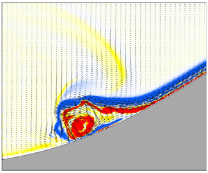



1. Introduction
Internal solitary waves (ISWs) are typical nonlinear waves that occur in the stratified ocean, with a maximum amplitude located in the oceanic interior; these waves can propagate over long distances after generation while maintaining their basic wave characteristics (Grimshaw et al. Reference Grimshaw, Ostrovsky, Shrira and Stepanyants1998, Reference Grimshaw, Pelinovsky, Talipova and Kurkina2010; Helfrich & Melville Reference Helfrich and Melville2006; Alford et al. Reference Alford, Lien, Simmons, Klymak, Ramp, Yang, Tang and Chang2010; Ramp et al. Reference Ramp, Park, Yang, Bahr and Jeon2019). They are characterized by large amplitudes, strong velocities, strong shear and short periods, which can draw the thermocline downwards or upwards for tens to hundreds of metres, resulting in surface velocities of 1–2 m s $^{-1}$ (Pinkel Reference Pinkel2000; Alford et al. Reference Alford, Lien, Simmons, Klymak, Ramp, Yang, Tang and Chang2010; Farmer et al. Reference Farmer, Alford, Lien, Yang, Chang and Li2011; Huang et al. Reference Huang, Chen, Zhao, Zhang, Zhou, Yang and Tian2016). Due to these characteristics, ISWs have an important impact on the safety of underwater vehicles and marine structures (Song et al. Reference Song, Teng, Gou, Lu, Shi, Xiao and Qu2011; Wang et al. Reference Wang, Zhou, Wang and You2018, Reference Wang, Huang, Zhao, Zheng, Yang and Tian2022). As ISWs shoal and break over the seabed topography, they release considerable amounts of energy that can promote local turbulent mixing and the resuspension of sediments and nutrients in the ocean (Sandstrom & Elliott Reference Sandstrom and Elliott1984; Reeder, Ma & Yang Reference Reeder, Ma and Yang2011; Boegman & Stastna Reference Boegman and Stastna2019). ISWs are also an effective pathway for transferring energy from large-scale barotropic tides to small-scale turbulence, and cumulatively this energy is an integral part of the oceanic energy budget (Bourgault & Kelley Reference Bourgault and Kelley2003; Zhang et al. Reference Zhang, Huang, Yang, Zhao, Wang, Yuan and Tian2023).
The ISWs generated by barotropic tides over varying seabed topographies are common in marginal seas worldwide (Jackson Reference Jackson2007). The onshore propagation of ISWs interacts with the seabed topography and eventually dissipates on the continental shelf slope (Lamb Reference Lamb2014; Davis et al. Reference Davis, Arthur, Reid, Rogers, Fringer, DeCarlo and Cohen2020; Jones et al. Reference Jones, Ivey, Rayson and Kelly2020). In the process of wave shoaling, fission, polarity conversion and other evolutionary processes will occur (Orr & Mignerey Reference Orr and Mignerey2003; Ramp et al. Reference Ramp, Yang, Jan, Chang, Davis, Sinnett, Bahr, Reeder, Ko and Pawlak2022; Sinnett et al. Reference Sinnett, Ramp, Yang, Chang, Jan and Davis2022), as well as the breaking and mixing process caused by shear instability, convection instability and benthic boundary layer instability (Moum et al. Reference Moum, Farmer, Smyth, Armi and Vagle2003; Barad & Fringer Reference Barad and Fringer2010; Lien et al. Reference Lien, Henyey, Ma and Yang2014; Boegman & Stastna Reference Boegman and Stastna2019; Xu & Stastna Reference Xu and Stastna2020; Chang et al. Reference Chang2021). All these processes promote the dissipation of ISWs and transform their energy into microscale turbulence.
Due to the importance of ISW shoaling and breaking, how to characterize the breaking of ISWs in terms of predetermined factors has become a hot topic. Several studies have analysed the shoaling, breaking and energy distribution of ISWs on uniform slopes (Helfrich Reference Helfrich1992; Michallet & Ivey Reference Michallet and Ivey1999; Boegman, Ivey & Imberger Reference Boegman, Ivey and Imberger2005; Bourgault & Kelley Reference Bourgault and Kelley2007; Lamb & Nguyen Reference Lamb and Nguyen2009; Aghsaee, Boegman & Lamb Reference Aghsaee, Boegman and Lamb2010; Sutherland, Barrett & Ivey Reference Sutherland, Barrett and Ivey2013; Carr et al. Reference Carr, Stastna, Davies and van de Wal2019; Nakayama et al. Reference Nakayama, Sato, Shimizu and Boegman2019; Hartharn-Evans et al. Reference Hartharn-Evans, Carr, Stastna and Davies2021). Through laboratory experiments, Boegman et al. (Reference Boegman, Ivey and Imberger2005) found that the breaking mechanism of internal waves depends on the ratio of the topographic slope to the incident wave slope. Referring to the breaking type of surface waves, they classified internal wave breaking into spilling, plunging and collapsing, and introduced the internal Iribarren number ( $Ir$) to delineate different breaking types:
 \begin{equation} Ir=\frac{s}{\sqrt{s_w}}, \end{equation}
where  $s$ is the topographic slope,
 $s_w=a/L_w$ is the wave slope,
 $a$ is the incident wave amplitude, and
 $L_w$ is the wavelength. Sutherland et al. (Reference Sutherland, Barrett and Ivey2013) adjusted and expanded the classification scheme of ISW breaking, which can be separated into no breaking, surging breaking, collapsing breaking, plunging breaking and plunging–collapsing breaking. By analysing previous experimental and numerical results, Nakayama et al. (Reference Nakayama, Sato, Shimizu and Boegman2019) defined a dimensionless parameter based on weakly nonlinear theory (KdV theory)
 $B_{ISW}=(s/s_w)\,Re_{ISW}^2$, which depends on the wave slope, topographic slope and wave Reynolds number (
 $Re_{ISW}\equiv \alpha a h_0 / \nu$, where
 $\alpha$ is the coefficient of the nonlinear term in the KdV equation,
 $h_0$ is the harmonic mean of the water depth, and
 $\nu$ is the kinematic viscosity). Plunging breaking occurs when
 $B_{ISW}>7\times 10^6$, while collapsing breaking occurs when
 $B_{ISW}<7\times 10^6$. Hartharn-Evans et al. (Reference Hartharn-Evans, Carr, Stastna and Davies2021) combined numerical simulations and experiments to explore the influence of stratification on the shoaling and breaking of ISWs, and found that surface stratification (density gradient throughout the upper layer) can inhibit plunging, while a broad tanh profile can simultaneously inhibit collapsing and plunging.
When an ISW breaks on a slope, part of the energy dissipates locally, and part is reflected. Regarding the reflection coefficient on uniform slopes, the experimental results of Helfrich (Reference Helfrich1992) and Michallet & Ivey (Reference Michallet and Ivey1999) showed that the ratio of reflected energy generated by ISWs impinging on the slope to total energy depends on the wavelength and topographic scale ratio. The numerical simulation of Bourgault & Kelley (Reference Bourgault and Kelley2007) showed that Michallet & Ivey (Reference Michallet and Ivey1999) underestimated the reflection coefficient due to ignoring the friction effect, and proposed a parametrization scheme dependent on  $Ir$, namely
 $R=1-{\rm e}^{-Ir/Ir_0}$, where
 $Ir_0=0.78\pm 0.02$ (95 % confidence intervals). Lamb & Nguyen (Reference Lamb and Nguyen2009) combined the available potential energy flux with the kinetic energy flux to calculate the reflection coefficient, and found that compared to the approximate calculation method of Bourgault & Kelley (Reference Bourgault and Kelley2007), the correct estimation of available potential energy flux could reduce the predicted reflection coefficient by a maximum of 0.1. Aghsaee et al. (Reference Aghsaee, Boegman and Lamb2010) believed that the calculation of the reflection coefficient at the toe of the slope would ignore the energy dissipation caused by viscosity before incident wave breaking and after reflection wave generation. The reflection coefficient based on the breaking point has been introduced, and the coefficient
 $Ir_0$ of the parametrized scheme of Bourgault & Kelley (Reference Bourgault and Kelley2007) was revised to 0.65.
The breaking location of ISWs on slopes can be predicted by the initial stratification conditions and the incident wave parameters (Helfrich Reference Helfrich1992; Vlasenko & Hutter Reference Vlasenko and Hutter2002; Aghsaee et al. Reference Aghsaee, Boegman and Lamb2010; Sutherland et al. Reference Sutherland, Barrett and Ivey2013; Cavaliere et al. Reference Cavaliere, la Forgia, Adduce, Alpers, Martorelli and Falcini2021). The experimental results of Helfrich (Reference Helfrich1992) showed that breaking occurs when the non-dimensional wave amplitude ( $a/(h_b-h_m)$, where
 $h_b$ is the water depth at the breaking point, and
 $h_m$ is the depth of the undisturbed interface) exceeds 0.4. Vlasenko & Hutter (Reference Vlasenko and Hutter2002) proposed an ISW breaking criterion that is dependent on the topographic slope (represented by slope angle
 $\gamma =\arctan (s)$), which was based on the selection of stratification conditions, topography and wave parameters of the Andaman Sea and Sulu Sea:
 \begin{equation} \frac{a}{h_b-h_m}\geq\frac{0.8^{{\circ}}}{\gamma }+0.4. \end{equation}
For the prediction of the maximum interfacial descent ( $a_{max}$) at the breaking depth, Sutherland et al. (Reference Sutherland, Barrett and Ivey2013) approximated the waveforms of internal waves before breaking into a right triangle shape (especially for plunging–collapsing breaking). Assuming that the area of the right triangle (the volume per unit width of the upper layer fluid below the initial depth of the interface) is equal to the approximate area of the incident wave (
 $S_{ISW}=aL_w$), a prediction formula for
 $a_{max}$ has been established:
 \begin{equation} a_{max}=\sqrt{4saL_{sw}}, \end{equation}
where  $L_{sw}$ is half of the width at half-amplitude. Based on the analysis method of Sutherland et al. (Reference Sutherland, Barrett and Ivey2013), Cavaliere et al. (Reference Cavaliere, la Forgia, Adduce, Alpers, Martorelli and Falcini2021) modified the area of the initial wave by using extended KdV and Miyata–Choi–Camassa theories to obtain the prediction formula of the breaking location and depth.
For the evolution of ISWs over submerged obstacles (Wessels & Hutter Reference Wessels and Hutter1996; Sveen et al. Reference Sveen, Guo, Davies and Grue2002; Chen Reference Chen2007, Reference Chen2009; Sutherland, Keating & Shrivastava Reference Sutherland, Keating and Shrivastava2015), the blockage parameter ( $\zeta$) was identified as another important parameter:
 \begin{equation} \zeta=\frac{a+h_1}{h_1+h_2-H_r}, \end{equation}
where  $h_1$ and
 $h_2$ represent the upper and lower water depths, respectively, and
 $H_r$ represents the height of the ridge. The laboratory experiment of Sveen et al. (Reference Sveen, Guo, Davies and Grue2002) studied the interaction of ISWs with triangular ridges, classifying the degree of interaction (as weak, moderate or strong) according to the blockage parameter and the dimensionless velocity over the ridge crest. Strong interaction occurs when
 $\zeta >0.6$, and the breaking of ISWs results in intense turbulent mixing. Chen (Reference Chen2009) also described the degree of interaction in terms of wave energy based on the blockage parameter, and developed a statistical method to classify the types of interaction (Chen Reference Chen2010). For mode-2 ISWs under symmetric stratification (
 $h_1=h_2$), a similar blockage parameter (
 ${a}/{(h_2-h_t-H_r)}$, where
 $h_t$ is the pycnocline half-width) is used to classify the wave–ridge interaction strength, with a parameter exceeding 0.5 indicating wave breaking conditions (Deepwell et al. Reference Deepwell, Stastna, Carr and Davies2017, Reference Deepwell, Stastna, Carr and Davies2019). For the evolution and breaking of ISWs over a ridge, Hsieh et al. (Reference Hsieh, Hwang, Hsu and Cheng2015) and Zhu et al. (Reference Zhu, Wang, Avital, Tang and Williams2016) analysed the variation in wave parameters and energy through numerical simulations, and Lin et al. (Reference Lin, Luo, Yu, Song and Yuan2021) analysed the breaking structure and dissipation through laboratory experiments. In the other case, as the ISW passes over a small-amplitude, broad ridge, instability occurs near the crest of the topography in the form of a roll-up of vorticity, whereas the dissipation of wave energy is minimal (Harnanan, Soontiens & Stastna Reference Harnanan, Soontiens and Stastna2015; Harnanan, Stastna & Soontiens Reference Harnanan, Stastna and Soontiens2017).
The energy distribution of ISWs on the ridge exhibits both reflective and transmissive characteristics, which distinguishes it from the slope intersecting the pycnocline in the two-dimensional (2-D) case. Chen (Reference Chen2009) used the blockage parameter to characterize the transmitted and reflected energy. Zhu et al. (Reference Zhu, Wang, Avital, Tang and Williams2016) described the varying trends of energy dissipation, transmission and reflection coefficients through the empirical formula of multiplying the blockage parameter and nonlinear parameter. Sutherland et al. (Reference Sutherland, Keating and Shrivastava2015) non-dimensionalized the incident amplitude through the critical amplitude (dependent on topography and initial stratification), and provided a parametrized scheme for calculating the reflection and transmission coefficients.
The breaking and energy distribution of ISWs over a ridge have been investigated in previous studies based on laboratory experiments and numerical simulations. However, when selecting the interaction degree factor, the influence of the ridge height was mainly considered without considering the ridge slope simultaneously. At the field scale, the fractal structure of the seafloor gives rise to the presence of multiscale superposition of the topography. For example, gentler shelf slope areas have average slope about 0.03 to 0.07 (Cacchione, Pratson & Ogston Reference Cacchione, Pratson and Ogston2002), which is much larger than the wavelength scale of ISWs. In the case of steeper slopes, the characteristic width of the bumpy topography, underwater banks and seamounts are comparable to the wavelengths of typical large-amplitude ISWs (Smith Reference Smith1988; Wessel Reference Wessel2001; Vlasenko Reference Vlasenko2005; Xie et al. Reference Xie, He and Cai2019). The variable horizontal and vertical scales of the seafloor result in a broad range of dimensionless parameters that control the type of interaction between the ISW and topography (table 1). Consequently, it is imperative to examine the combined effects of variations in topographic height and slope. This paper focuses on the case where the horizontal scale of the topography is comparable to the ISW wavelength, and the topographic height is comparable to the total water depth, a condition under which the topography has the most noticeable effect on the ISW (Sveen et al. Reference Sveen, Guo, Davies and Grue2002; Sutherland et al. Reference Sutherland, Keating and Shrivastava2015).
The dimensionless parameter ranges in this experiment and a comparison between the predominant ranges of dimensionless parameters in laboratory scale and field scale. The parameter ranges in laboratory scale and field scale refer to figures and tables from previous studies (Michallet & Ivey Reference Michallet and Ivey1999; Sveen et al. Reference Sveen, Guo, Davies and Grue2002; Boegman et al. Reference Boegman, Ivey and Imberger2005; Vlasenko Reference Vlasenko2005; Chen Reference Chen2009; Aghsaee et al. Reference Aghsaee, Boegman and Lamb2010; Alford et al. Reference Alford, Lien, Simmons, Klymak, Ramp, Yang, Tang and Chang2010; Bourgault, Janes & Galbraith Reference Bourgault, Janes and Galbraith2011; Sutherland et al. Reference Sutherland, Barrett and Ivey2013, Reference Sutherland, Keating and Shrivastava2015; Xie, He & Cai Reference Xie, He and Cai2019; Davis et al. Reference Davis, Arthur, Reid, Rogers, Fringer, DeCarlo and Cohen2020; Ghassemi, Zahedi & Boegman Reference Ghassemi, Zahedi and Boegman2021; Hartharn-Evans et al. Reference Hartharn-Evans, Carr, Stastna and Davies2021).

Regarding laboratory experiments, the research still lacks a complete description of the wave–ridge interaction. In this paper, a series of processes, such as shoaling, breaking, transmission and reflection of the interaction between the ISW and the Gaussian topography, are captured completely by measuring the velocity field in a large region. The laboratory experiments were used to systematically analyse the breaking types and dynamic processes of the wave–ridge interaction to study the energy distribution, the spatiotemporal structure of the turbulence, and the details of the breaking process. A dimensionless parameter that accounts for both ridge height and slope is introduced to characterize the degree of interaction. The study of the distribution trends of the breaking type, breaking position and breaking depth is helpful in analysing the mixing process, sediment resuspension process, and transport of material caused by internal waves. It can also be used to assist in the exploration of the energy distribution, which is useful for analysing the effect of internal waves on the oceanic energy budget.
The paper is structured as follows. The experimental set-up, definition and calculation of the basic parameters are introduced in § 2. In § 3, the basic characteristics and evolution of the ISW over the ridge are evaluated, and the breaking type and breaking time scale are analysed. In § 4, a method for predicting the maximum interface descent that can reflect the shoaling effect of internal waves is given. In addition, a prediction scheme for the type of breaking and energy distribution based on the maximum interface descent is also given. Finally, the results are summarized in § 5.
2. Experimental methods
2.1. Experimental set-up
Mode-1 depression ISWs were generated in an approximately two-layer stratified fluid using the standard lock-release method (Kao, Pan & Renouard Reference Kao, Pan and Renouard1985). The flume was 6 m long, 0.5 m high and 0.24 m wide (figure 1). The left-hand side of the flume was a wave-generating region. Before entering the observation region, the fluid that was released by the lock-release method had evolution distance up to 2 m, which made it adaptable to the characteristics inherent to an ISW. The centre of the flume was an experimental observation region with a 2-D Gaussian ridge, and the right-hand side was placed with a uniform slope for wave absorption.
(a) Schematic diagram of the experimental set-up (not to scale). The fluids in the upper and lower layers are shown in light and dark blue, respectively. The green area and the red dotted box represent the particle image velocimetry observation regions for the large-region experiments and high-resolution experiments, respectively. The left-hand side is a wave-generating region by the standard lock-release method, and  $h_c$ is the collapse height. Here,
 $H_r$ and
 $L_s$ represent the height and characteristic length of the Gaussian ridge, respectively. The right-hand side is placed with a uniform slope for wave absorption (the slope is 0.33, with no porosity). (b) The measured density profile before the H2S1 run. The measured values are represented by circles, while the fitted results are represented by black lines.

The Gaussian ridge has constant height  $H_r=16$ cm and a variable standard deviation of the Gaussian function (
 $\sigma$) to account for changes in the topographic length and slope. Following the definition of Hult, Troy & Koseff (Reference Hult, Troy and Koseff2011), the topographic characteristic slope was defined as
 $s=H_r/2\sigma$. The characteristic length of the ridge was defined as
 $L_s=2\sigma$. Three topographic characteristic slopes were designed in the experiment, 0.20, 0.33 and 0.50, which are comparable to bathymetric slopes 0.07–0.5, where enhanced diapycnal diffusivities have been observed (Kunze & Sanford Reference Kunze and Sanford1996; Toole et al. Reference Toole, Schmitt, Polzin and Kunze1997). The densities of the two-layer stratified fluid remained constant, with density 1020 kg m
 $^{-3}$ in the upper layer (
 $\rho _1$) and 1040 kg m
 $^{-3}$ in the lower layer (
 $\rho _2$). The depth of the upper layer (
 $h_1$) remained constant at 4 cm in all cases, and the lower layer (
 $h_2$) varied from 20 to 32 cm. The background stratification was measured with a conductivity probe before each experiment. The thickness of the interface
 $2h_t$ was obtained by fitting a hyperbolic tangent function to the measured profile (
 $\bar {\rho }(z)=\rho _0-({\Delta \rho }/{2})\tanh ({(z-z_0)}/{h_t})$, where
 $\rho _0=1030$ kg m
 $^{-3}$ is the reference density,
 $\Delta \rho =\rho _2-\rho _1=20$ kg m
 $^{-3}$,
 $z_0=h_1$, and
 $h_t$ is obtained by fitting). In this experiment,
 $h_t$ ranged from 0.007 to 0.012 m. The width of the lock region was 20 cm, and the collapse height ranged from 4 to 24 cm (
 $h_c$), depending on the depth of the lower layer and the stratification conditions. The experimental conditions were a combination of different stratification conditions, topographic slopes and collapse heights, with a total of 60 experimental groups (table 2).
Experimental parameters, where  $H$ is the total water depth,
 $s$ is the topographic slope,
 $h_c$ is the collapse height,
 $a$ is the incident wave amplitude, and
 $h_1$ is the depth of the upper layer. The letters in the last column indicate the interaction type (corresponding to
 $h_c$): N for no breaking, F for fission, T for transition P for plunging, PC for plunging–collapsing. The asterisks on
 $h_c$ values indicate two additional cases of high-resolution experiments.

Particle image velocimetry (PIV) was used to measure the velocity field of the interaction between the ISWs and the Gaussian ridge. For large-region measurement experiments, three lasers (power 3 W, wavelength 532 nm) and three CCD cameras (Basler acA1920-155  $\mathrm {\mu }$m) formed an experimental measuring range of up to 2.6 m (larger than the longest topography in this experiment), which could fully capture the incidence, shoaling, breaking, reflection and transmission processes of the ISWs. Images were taken at 50 Hz using 1920 × 1200 pixels for each CCD camera, to give spatial resolution 0.6 mm.
We used PIVlab (Thielicke Reference Thielicke2014; Thielicke & Stamhuis Reference Thielicke and Stamhuis2014; Thielicke & Sonntag Reference Thielicke and Sonntag2021), a MATLAB program package, to analyse the raw images. For cross-correlation algorithms, the multi-pass starting from the interrogation area 64 × 64 pixels, ending with a smaller interrogation area of 24 × 24 pixels with a 50 % overlap, resulted in spatial resolution of the flow field at 7.2 mm (table 3). Consult Thielicke (Reference Thielicke2014) to estimate the magnitude of errors for the PIV analysis (detailed information is provided in § 1 of the supplementary material available at https://doi.org/10.1017/jfm.2024.692). The relative errors of the flow velocity are 0.8 % and 3.8 % for bias error and random error, respectively. According to Dalziel et al. (Reference Dalziel, Carr, Sveen and Davies2007), the particle displacement caused by the index of refraction is a maximum of 1.1 mm (less than 2 pixels), based on the maximum buoyancy frequency in this experiment ( $N^2=11$ s
 $^{-2}$).
Parameters of PIV analysis.

To assess the breaking and energy dissipation of ISWs on a ridge with greater precision, two additional cases of high-resolution experiments were conducted (as indicated by the asterisks in table 2, the experimental set-up was the same as that for the large-region experiment). However, the shooting area is limited to the upstream slope, as indicated by the red box in figure 1. Images were taken at 128 Hz using a 4096 × 3072 pixels CCD camera, to give spatial resolution 0.1 mm. The minimum interrogation area is 20 × 20 pixels with a 50 % overlap, resulting in the spatial resolution of the flow field being 1.1 mm. The relative errors of the flow velocity are 0.2 % and 0.9 % for bias error and random error, respectively (table 3).
2.2. Calculation method
The ISW stable propagation on a flat bottom prior to shoaling allowed identification of the waveform and calculation of basic physical quantities such as amplitude, wavelength and wave speed by schlieren (Wallace & Wilkinson Reference Wallace and Wilkinson1988; Dalziel et al. Reference Dalziel, Carr, Sveen and Davies2007; Raffel Reference Raffel2015; Settles & Hargather Reference Settles and Hargather2017). The ISW propagation experiment without ridges was carried out to obtain wave parameters using background stripe schlieren (§ 2 of the supplementary material provides details on schlieren). The amplitude of the wave was determined by the maximum vertical displacement of the waveform, and the wavelength was determined by the ratio of the integral of the wave profile to the amplitude:
 \begin{equation} L_w=\frac{1}{a}\int_{-\infty}^{+\infty}\eta(x)\,\mathrm{d}\kern0.07em x. \end{equation}
The wave speed ( $C_p$) was determined by the distance of wave propagation within a given time. The incident amplitude, internal wave phase speed and characteristic wavelength were non-dimensionalized by the upper layer depth, linear phase speed (
 $C_0$) and harmonic mean of the water depth (
 $h_0= h_1h_2/(h_1+h_2)$), respectively.
Dimensionless parameters related to this experiment were determined by the wave parameters and the topography parameters, as shown in table 1. Dimensionless amplitudes include both weak and strong nonlinearities. The blockage parameter ranges from the weak interaction of waves that are almost unaffected to the strong interaction with wave breaking and mixing (Sveen et al. Reference Sveen, Guo, Davies and Grue2002; Chen Reference Chen2009). The character of ISW breaking can be covered by  $Ir$ (Aghsaee et al. Reference Aghsaee, Boegman and Lamb2010; Sutherland et al. Reference Sutherland, Barrett and Ivey2013). The experiments include scales of topographic length larger and smaller than the characteristic wavelength.
Kinetic energy is calculated as
 \begin{equation} E_k(x,z,t)=\tfrac{1}{2}\rho_0[{u(x,z,t)}^2+{w(x,z,t)}^2], \end{equation}
where  $\rho _0$ is the reference density, and
 $u$ and
 $w$ are the horizontal velocity and vertical velocity retrieved from the PIV measurement, respectively.
The energy density is calculated by the vertical integral of the kinetic energy:
 \begin{equation} E_{kz}(x,t)=\int_{0}^{H}{E_k(x,z,t)\,\mathrm{d} z}, \end{equation}
where  $H=(h_1+h_2)$ is the total water depth.
Following the method of Michallet & Ivey (Reference Michallet and Ivey1999), the kinetic and available potential energies are approximated for ISWs with small wave amplitudes (Bogucki & Garrett Reference Bogucki and Garrett1993); thus the total energy can be calculated as
 \begin{equation} E=2C_p\int_{t_1}^{t_2}{E_{kz}(X,t)\,\mathrm{d} t}. \end{equation}
The truncation of  $t_1$ and
 $t_2$ is 1 % of the maximum vertical integral of the energy, and
 $X$ is a specific horizontal position. To avoid the influence of shoaling and breaking on the energy calculation, the incident wave energy was calculated before the interaction between the wave and ridge, and the reflected and transmitted wave energies were calculated after the ISW stabilized (Michallet & Ivey Reference Michallet and Ivey1999). The calculated position of the incident wave and reflected wave is
 $X=-1.0$ m, and the transmitted wave is
 $X=1.0$ m (we define the horizontal position of the top of the ridge as
 $X = 0$ m). This distance is half the length of the longest topography (
 $s=0.2$,
 $\sigma =0.4$,
 $X=\pm 2.5\sigma$), where the transmitted and reflected waves have developed into stable waveforms.
Since the 2-D velocity field can be obtained by the PIV system, the direct method is used to calculate the spatial distribution of the turbulent kinetic energy (TKE) dissipation rate. Based on the isotropic assumption, it can be calculated by the 2-D velocity field (Doron et al. Reference Doron, Bertuccioli, Katz and Osborn2001):
 \begin{equation} \varepsilon=4\nu\left[\overline{\left(\frac{\partial u^\prime}{\partial x}\right)^2}+\overline{\left(\frac{\partial w^\prime}{\partial z}\right)^2}+\overline{\left(\frac{\partial u^\prime}{\partial x}\,\frac{\partial w^\prime}{\partial z}\right)}+\frac{3}{4}\,\overline{\left(\frac{\partial u^\prime}{\partial z}+\frac{\partial w^\prime}{\partial x}\right)^2}\right], \end{equation}
where  $u^\prime$ and
 $w^\prime$ are the fluctuation velocities (the instantaneous velocity measured by PIV is used in this experiment). The kinematic viscosity coefficient is
 $\nu =1.0\times {10}^{-6}$ m
 $^2$ s
 $^{-1}$ (at laboratory temperature 20
 $^{\circ }$C). According to Cowen & Monismith (Reference Cowen and Monismith1997) and Liao et al. (Reference Liao, Bootsma, Xiao, Klump, Hume, Long and Berg2009), 99 % of the dissipation will be included with finite differencing if the PIV grid size is smaller than
 $5.5l_0$ (where
 $l_0={({\nu ^3}/{\varepsilon })}^{{1}/{4}}$ is the Kolmogorov scale). Therefore, the high-resolution experiments are sufficient to estimate the TKE dissipation rate less than
 $8\times {10}^{-4}$ m
 $^2$ s
 $^{-3}$. However, numerous factors can lead to anisotropic turbulence in the case of breaking interfacial waves. The estimates of dissipation obtained using various methods (dissipation from 2-D PIV, stereo-PIV, acoustic Doppler velocimeter data, and log-law data), parts of which rely on assumptions of isotropy, provide the same order-of-magnitude values (Zahedi Reference Zahedi2021).
3. Results
3.1. Evolution process
In this subsection, a series of dynamic processes, such as shoaling, breaking, transmission and reflection, as well as the evolution of wave energy, are presented through several sets of typical experiments.
The superposition of the vorticity and flow fields is presented in figure 2 to provide a detailed view of the structure of the breaking process. As shown in figure 2, the process of interaction of plunging–collapsing breaking can be divided into the following four stages (sketches of each stage are presented in Appendix A).
(1) In figure 2(a), the wave trough propagates to the toe of the slope, at which time the bulk of the wave starts to contact the topography. A vorticity structure forms at the interface due to the mode-1 velocity field of the depressed ISW.
(2) Due to topographic modulation, the propagation speed of the trailing edge of the wave is greater than that of the wave trough, making the trailing edge steeper. The maximum horizontal velocity of the upper layer moves to the trailing edge of the wave. The waveform on the left-hand side of the ridge is parallel to the topography, the downslope velocity of the lower layer increases, and part of the wave is transmitted through the top of the ridge (figure 2b).
(3) The ISW becomes unstable, and the velocity of the water particle on the trailing edge of the wave exceeds the wave speed (Vlasenko & Hutter Reference Vlasenko and Hutter2002; Lien et al. Reference Lien, Henyey, Ma and Yang2014), resulting in convective instability and flow separation at the benthic boundary layers in the adverse pressure gradient region (red arrow in figure 2c). The two types of instability processes generate distinct positive vorticities above and below the pycnocline.
(4) In figures 2(d,e), the ISW breaks, and the vortices resulting from the initial instability split into smaller scales, generating strong turbulent mixing on the ridge. Simultaneously, generated reflected waves (figure 2e, positive vorticity,
 $x=-0.6$ m) and transmitted waves (figure 2d, negative vorticity, $x=0.7$ m) have left the topography. The transmitted wave is followed by a significant dispersive wave tail, whereas the reflected wave is not. In the weak interaction with a small blockage parameter, ISWs do not break, only the waveform is modulated by the topography, and no reflected wave generation occurs.


Evolution of the interaction between ISWs and topography. The image is a superposition of the vorticity and flow fields for values of  $t$ (a) 0 s, (b) 3.0 s, (c) 5.0 s, (d) 11.0 s, (e) 11.0 s, ( f) 28.2 s. The experimental conditions are as follows: the water depth is
 $H=0.28$ m, the slope is
 $s=0.50$, and the incident wave amplitude is
 $a=0.075$ m. In (a) and (b), the yellow dots represent the waveforms identified by the vertical position of the extremes of the velocity shear in each column, and the red lines represent the composite Froude number. The red dashed lines in (b) and (e) represent the depth of the incident amplitude. The red arrow in (c) indicates the adverse pressure gradient region.

For ISWs breaking, not only convective instability and bottom boundary instability are present, but also Kelvin–Helmholtz billows generated by shear instability can be identified via high-resolution experiments (figure 3). During the upwelling of the fluid mass induced by plunging in plunging–collapsing breaking, strong flow still exists in the lower layer. Consequently, billows induced by strong shear are continuously generated initially as 2-D vortices and subsequently split into three-dimensional (3-D) states (red arrows in figure 3). In this instance, the billow was generated at a location different from that in previous observations, with the billow appearing only at the trailing edge of the wave (Moum et al. Reference Moum, Farmer, Smyth, Armi and Vagle2003; Chang et al. Reference Chang2021). For ISWs, the breaking threshold is  ${L_x}/{2L_w}=0.86$, where
 $L_x$ is the horizontal length of the region in which the Richardson number is less than 0.25 (Fructus et al. Reference Fructus, Carr, Grue, Jensen and Davies2009; Barad & Fringer Reference Barad and Fringer2010; Carr, King & Dritschel Reference Carr, King and Dritschel2011). The numerical simulation of Xu, Stastna & Deepwell (Reference Xu, Stastna and Deepwell2019) indicated that when
 ${L_x}/{2L_w} \approx 0.88$, the shear instability occurs spontaneously, without any externally imposed physical noise. In the absence of direct density measurements in this experiment, visual vortex development was relied upon for this part of the analysis of the process of shear instability and Kelvin–Helmholtz billows. According to the definition of Carr et al. (Reference Carr, Franklin, King, Davies, Grue and Dritschel2017), the dimensionless billow wavelength in figure 3(b) is
 ${\lambda _b}/{2h_t}=2.0$ (
 $h_t=0.8$ cm), and the dimensionless vertical extent of the billow at
 $x=-0.09$ m is
 ${L_b}/{2h_t}=0.73$. Both of these scales are significantly smaller than the billow at the trailing edge of the wave as shown in Carr et al. (Reference Carr, Franklin, King, Davies, Grue and Dritschel2017, tables 2 and 3). This may be due to the wavelength of the fastest growing wave of disturbance being determined by velocity shear and stratification (Xu Reference Xu2015).
The evolution vorticity field of plunging–collapsing breaking in high-resolution experiments,  $H=0.24$ m,
 $s=0.50$ and
 $a=0.064$ m, for (a)
 $t=13.7$ s, and (b)
 $t=14.9$ s. Red arrows indicate Kelvin–Helmholtz billows.

Figure 4 shows the evolution of ISWs over the ridge by using the vertical integral of the kinetic energy (2.3). In figure 4(a), with a small incident amplitude, the ISW will not break when it passes through the topography, but its propagation speed is clearly modulated by the topography. The wave speed slows at the top of the ridge, and gradually returns to a constant speed after passing over the ridge. As the lower water depth at the ridge becomes shallower, the shear at the interface is enhanced. The energy is decreased in the laminar flow by the viscosity, as there are no instability processes during the evolution. This leads to a significant decrease in the energy density after the wave passes over the ridge. In this case, following the usual definition for stratified shear flows, a Reynolds number is introduced as  $Re=\Delta u\,h_t/2\nu =88$, where
 $\Delta u$ is the velocity jump across the pycnocline when the wave trough passes over the top of the ridge. For
 $Re\le 100$, viscosity reduces the growth rate and damps the high wavenumber perturbations (Hogg & Ivey Reference Hogg and Ivey2003; Fructus et al. Reference Fructus, Carr, Grue, Jensen and Davies2009).
Time series showing the vertical integral of kinetic energy along the length of the observation region. (a) The water depth is  $H=0.24$ m, the slope is
 $s=0.20$, and the incident wave amplitude is
 $a=0.019$ m. (b) The water depth is
 $H=0.28$ m, the slope is
 $s=0.50$, and the incident wave amplitude is
 $a=0.075$ m. The black dashed lines represent the maximum value of the energy density of different wave rays. The white dashed lines correspond to the five moments in figure 2. The square and triangle in (b) correspond to the start times (horizontal coordinates indicate the breaking position) of plunging breaking and collapsing breaking, respectively.

The experimental conditions in figure 4(b) are the same as in figure 2. The white dashed lines in figure 4(b) correspond to the five moments in figure 2, and the black dashed lines represent the positions of the maximum energy density of different wave rays. The ISW will be broken when interacting strongly with the ridge, generating transmitted and reflected waves, accompanied by mode-2 ISW generation. The wave speed was calculated by the slope of the maximum energy density curve, and the incident wave speed was 0.104 m s $^{-1}$, the transmitted wave speed was 0.093 m s
 $^{-1}$, and the reflected wave speed was 0.091 m s
 $^{-1}$. The propagation speed of the mode-2 wave measured in the experiment was 0.0283 m s
 $^{-1}$. The three-layer model of Yang et al. (Reference Yang, Fang, Tang and Ramp2010) was used to evaluate the propagation speed of mode-2 solitary waves. Taking the middle layer thickness as 2.4 cm (
 $2h_t$), the theoretical calculation result was 0.0299 m s
 $^{-1}$, which was consistent with the experimental result. The energy of this mode-2 ISW (calculated by multiplying the kinetic energy integral for
 $x = 0.63\unicode{x2013}0.73$ m in figure 2( f) by 2) is 0.42 % of the incident wave energy.
3.2. Breaking types
The ISW shoaling on the slope has two typical characteristics: (1) the trailing edge of the wave becomes steeper; (2) the lower layer fluid flows downwards and increases in velocity under the compression of the wave and topography (figure 2b) (La Forgia, Adduce & Falcini Reference La Forgia, Adduce and Falcini2018). As shown in figures 2(a–c), the cumulative effect of nonlinearity in a shoaling ISW leads to a steepening and overturning of the rear wave face (Vlasenko & Hutter Reference Vlasenko and Hutter2002). Because the ridge does not coincide with the pycnocline, the varying rate of the stratification nonlinear coefficient is determined by a combination of ridge slope and height. Fluid can be replenished from the other side of the ridge during shoaling (the height of the ridge can adjust the width of the lower layer channel), making the velocity of the lower fluid layer much higher than that of shoaling on the uniform slopes. Therefore, the ridge height and slope are two important parameters in controlling the breaking type.
The shoaling of ISWs on uniform slopes is regulated by the wave slope and the topographic slope, resulting in plunging breaking, collapsing breaking, surging breaking, plunging–collapsing breaking and fission (Boegman et al. Reference Boegman, Ivey and Imberger2005; Aghsaee et al. Reference Aghsaee, Boegman and Lamb2010; Sutherland et al. Reference Sutherland, Barrett and Ivey2013; Nakayama et al. Reference Nakayama, Sato, Shimizu and Boegman2019). Given that breaking on uniform slopes has been defined clearly, the type of breaking on ridges is classified in terms of the dynamic processes of shoaling on uniform slopes. However, different from the uniform slope, the wave–ridge interaction not only has shoaling breaking and reflection, but also has a transmission process when passing through the ridge (Sveen et al. Reference Sveen, Guo, Davies and Grue2002; Chen Reference Chen2009; Sutherland et al. Reference Sutherland, Keating and Shrivastava2015). The interaction types were classified into the following five categories by analysing the experimental data (figure 5, plus sketches in § 3 of the supplementary material).
(1) Weak interaction. When
$\zeta < 0.5$, the waveform is almost unaffected by the ridge or is slightly deformed.(2) Fission. This occurs when both the slope and the incident amplitude are smaller. Significant fluctuations at the top of the ridge (figure 5a) cause alternating positive and negative vorticity at the interface (figure 5b); meanwhile, the bulk of the wave energy is transmitted past the ridge.
(3) Transition. There is a transition state between ISW breaking and no breaking. During the shoaling process, the trailing edge of the wave becomes steeper and almost perpendicular to the horizontal direction. However, simultaneously, the tail of the wave is located close to the top of the ridge (figure 5c), and the cumulative effect of nonlinearity no longer continues, so the trailing edge of the wave does not reach an overturned state when it passes over the ridge topography. In this state, if the incident amplitude or the topographic slope is increased, breaking will occur. This process does not occur in the interaction of ISWs with uniform slopes, where the continued cumulative effect of nonlinearity will cause convective instability (Boegman et al. Reference Boegman, Ivey and Imberger2005; Sutherland et al. Reference Sutherland, Barrett and Ivey2013).
(4) Plunging. The rear face of the wave overturns, resulting in convective instability in the horizontal direction, leading to plunging breaking. This breaking process is dominated by the dynamics on the pycnocline and is independent of the benthic boundary dynamics. The vortex at the top of the ridge represents the flow separation of the lower layer fluid around the topography without encountering the pycnocline.
(5) Plunging–collapsing. The rear face of the wave overturns, and the separation bubble is generated on the ridge, resulting in plunging–collapsing breaking, similar to the same breaking type on a uniform slope (Aghsaee et al. Reference Aghsaee, Boegman and Lamb2010; Sutherland et al. Reference Sutherland, Barrett and Ivey2013) and the strong interaction of the mode-2 ISW with a narrow ridge (Deepwell et al. Reference Deepwell, Stastna, Carr and Davies2017). In this condition,
$\zeta > 0.75$, and the maximum interfacial vertical displacement of the ISW increases significantly. The generated vortices in the benthic boundary layer and the rear face of the wave cause global breaking and mixing on the left-hand side of the ridge.


Different types of ISWs interact with ridges: (a,b) fission, (c,d) transition, (e, f) plunging breaking, and (g,h) plunging–collapsing breaking. The raw PIV images are shown in (a,c,e,g), with corresponding superimposed vorticity and flow fields in (b,d, f,h). Experimental conditions: (a)  $h_1=0.04$ m,
 $h_2=0.24$ m,
 $s=0.20$,
 $a=0.040$ m,
 $\zeta =0.65$,
 $Ir=0.65$; (c)
 $h_1=0.04$ m,
 $h_2=0.28$ m,
 $s=0.33$,
 $a=0.055$ m,
 $\zeta =0.58$,
 $Ir=0.95$; (e)
 $h_1=0.04$ m,
 $h_2=0.32$ m,
 $s=0.33$,
 $a=0.092$ m,
 $\zeta =0.63$,
 $Ir=0.82$; (g)
 $h_1=0.04$ m,
 $h_2=0.24$ m,
 $s=0.50$,
 $a=0.075$ m,
 $\zeta =0.91$,
 $Ir=1.30$.

Both plunging and plunging–collapsing breaking result in the dissipation of significant wave energy over the ridge. The analysis of the high-resolution flow field data to show the distribution of the TKE dissipation rate characteristics of wave breaking has greater significance. In figures 6(e–h), for plunging breaking, the high-value region of dissipation is generated primarily by velocity shear and wave breaking at the pycnocline in the interior, as well as by instability processes at the benthic boundary layer. A straightforward spatial delineation of the high-value dissipative areas can be identified within these two regions. Figures 6(e–g) correspond to the three peaks of the space integration of the  $\varepsilon$ time series in figure 6(h), respectively (represented by triangles). The initial peak is indicative of the generation of vortices at the bottom boundary, with dissipation originating primarily from this region, which accounts for 67 % of the space. By the second peak, the vortices generated at the bottom boundary broke into smaller vortex structures due to the instability in 3-D effects. The convection-induced plunging breaking, on the other hand, is sufficiently developed so that the dissipation percentage near the pycnocline is larger than that at the bottom boundary. (Due to the limitation of the observation region, some of the processes are already out of the field of view, which will underestimate the dissipation percentage near the pycnocline.) The third peak represents the maximum moment of dissipation for plunging breaking. Initially generated 2-D vortices are fully transformed into complex 3-D structures, with the dissipation percentage induced by the bottom boundary being 18 % greater than that near the pycnocline upstream of the ridge. In general, the dissipation percentage of the interior is lower than that of the bottom boundary during plunging breaking. This finding is similar to the results of Arthur & Fringer (Reference Arthur and Fringer2014), who found that the ratio of dissipation in the interior and bottom boundary is approximately
 $1\,:\,2$ for the ISW breaking on a uniform slope.
The evolution of the TKE dissipation rate of (a–d) plunging–collapsing breaking,  $H=0.24$ m,
 $s=0.50$,
 $a=0.064$ m, and (e–h) plunging breaking,
 $H=0.32$ m,
 $s=0.33$,
 $a=0.082$ m, for values of
 $t$ (a) 10.5 s, (b) 12.2 s, (c) 13.3 s, (e) 11.0 s, ( f) 13.8 s, (g) 15.7 s. (a–c,e–g) The spatial distribution of the TKE dissipation rate, which is dimensionless by the mean dissipation at the pycnocline of the wave trough before ISW breaking (
 $\varepsilon _0=1.4\times {10}^{-4}$ m
 $^2$ s
 $^3$ in plunging–collapsing breaking, and
 $\varepsilon _0=1.2\times {10}^{-4}$ m
 $^2$ s
 $^3$ in plunging breaking). (d,h) The black line is the time series of the spatial integration of the TKE dissipation rate, and the three triangles correspond to the three moments in (a–c,e–g). The purple and blue lines correspond to the time series of the spatial integration of TKE dissipation rate points in the matching coloured dashed boxes in (a) and (e), respectively. The box in (a) is fixed in time, while that in (e) moves with the flow.

For plunging–collapsing breaking, the dissipation at the pycnocline and the bottom boundary are superimposed on each other due to the ISW directly impinging upon the ridge. The high-value region is mainly distributed upstream of the ridge. Figures 6(a–c) correspond to the three typical moments of the space integration of  $\varepsilon$ in figure 6(d), respectively. In figure 6(a), the dissipation is attributed primarily to vortices generated by collapsing breaking (purple dashed rectangle) and enhanced shear (blue dashed rectangle). Subsequently, in figure 6(b), the dissipation due to collapsing breaking decreases, while the dissipation due to plunging breaking increases rapidly, resulting in a nearly one-fold increase in the total dissipation rate within 1.7 s (figure 6(d), 10.5–12.2 s). After the peak, the upwelling of the fluid mass induced by plunging (
 $x = -0.2$ to
 $-0.1$) maintains dissipation at a high value (figure 6c). The rate of increase in the dissipation rate of plunging–collapsing breaking is much greater than that of plunging breaking because the dissipation in plunging–collapsing breaking is caused by the sudden release of available potential energy accumulated upstream (figures 6a,b), whereas the dissipation in plunging breaking is attributed mainly to relatively slow overturning and bottom boundary instability.
3.3. Breaking criterion
The strength and breaking type of the wave–ridge interaction depends on the topography and wave parameters. Different interactions and breaking types are accompanied by different turbulent mixing and energy dissipation. In the experiment, the dimensionless parameters controlling ISW breaking were varied by adjusting the topographic slope, the stratification condition and the internal wave amplitude, totaling 60 sets of experimental data. This subsection considers the effect of both ridge height (introducing the blockage parameter) and the variation in the flow field during wave shoaling (introducing the Froude number) on ISW breaking. The effects of considering both ridge height and slope will be discussed in § 4.
Figure 7 considers the blockage parameter. When  $\zeta <0.5$, the ISW is almost unaffected by the ridge, and no breaking occurs. When the blockage parameter is sufficiently large (
 $\zeta >0.75$), only plunging–collapsing breaking occurs on the ridge. Four different interaction types may occur within the range
 $0.5<\zeta <0.75$.
Types of wave–ridge interactions in relation to  $\zeta$ and the maximum Froude number. The two horizontal dashed lines correspond to
 ${Fr}_{max}^2 = 0.40$ and
 ${Fr}_{max}^2 = 0.75$. The vertical dashed line corresponds to
 $\zeta = 0.75$. Crosses indicate no breaking, diamonds indicate fission, hollow circles indicate transition state, squares indicate plunging breaking, and triangles indicate plunging–collapsing breaking.

Convective instability appears in both plunging breaking and plunging–collapsing breaking (figures 5f,h), which resembles field observations as shown in Lien et al. (Reference Lien, Henyey, Ma and Yang2014, their figure 3) and Chang et al. (Reference Chang2021, their figure 2), and previous numerical simulations in the shoaling of internal waves (Lamb Reference Lamb2002, Reference Lamb2003; Lamb & Farmer Reference Lamb and Farmer2011; Rivera-Rosario et al. Reference Rivera-Rosario, Diamessis, Lien, Lamb and Thomsen2020, Reference Rivera-Rosario, Diamessis, Lien, Lamb and Thomsen2022). The convection in this experiment is generally stronger than the field observations because the topographic slope of the ocean is milder and the internal waves have sufficient time to adjust waveforms. In field observations, convective breaking is often examined by the along-wave current velocity exceeding the wave speed. Laboratory measurements provide the spatiotemporal structure of the velocity, and the character of the flow regimes of wave shoaling can be characterized by the composite Froude number (Maderich et al. Reference Maderich, Talipova, Grimshaw, Terletska, Brovchenko, Pelinovsky and Choi2010):
 \begin{equation} {Fr}^2=\frac{U_1^2}{g^\prime(h_1-\eta)}+\frac{U_2^2}{g^\prime(h_2+\eta)}, \end{equation}
where  $U_1$ and
 $U_2$ are the average horizontal velocities in the upper and lower layers, respectively, and
 $g^{\prime }$ is the reduced gravity. The maximum Froude number (
 ${Fr}_{max}$) increases significantly during the wave–ridge interaction (figures 2a,b), providing a clear distinction between the different interaction types (figure 7). In the case of no breaking,
 ${Fr}_{max}^2<0.40$. For fission and transition,
 $0.40<{Fr}_{max}^2<0.75$,
 $\zeta <0.75$. For plunging breaking,
 ${Fr}_{max}^2>0.75$. Plunging–collapsing breaking occurs for
 $\zeta >0.75$ and
 ${Fr}_{max}^2>0.40$.
3.4. Breaking time scale
Two kinds of dynamic processes lead to the breaking of the ISW interaction with the ridge: onshore overturning of the trailing edge (plunging breaking), and flow separation on the topography (collapsing breaking). To evaluate the breaking process, the trough of the wave reaching the toe of the slope ( $X = -L_s$) was taken as the starting point of time, and two types of time scales were calculated. The time needed for plunging breaking (
 $T_p$) is governed by the time when positive vorticity appears in the wave tail. The time needed for collapsing breaking (
 $T_c$) is governed by the time when the separated bubble contacts the pycnocline, leading to instability (Aghsaee et al. Reference Aghsaee, Boegman and Lamb2010).
Figure 8(a) shows the time scale of plunging breaking, which is dimensionless through the time ( $L_s/C_p$) of the internal wave propagating over the topographic scale (where
 $L_s$ is the horizontal distance from the toe to the top of the ridge) without the topography. Compared to the time of the internal wave passing through the topographic scale, the larger the blockage parameter or the smaller the Iribarren number, the earlier the trailing edge overturning leads to breaking. Figure 8(b) shows the ratio of plunging breaking and collapsing breaking time scales (
 $T_p/T_c$), revealing that the larger
 $\zeta$ and
 $Ir$, the earlier collapsing breaking occurs. The experimental results show that most collapsing breaking occurs earlier than plunging breaking. If plunging breaking occurs too early, then the maximum interfacial descent will dampen and be located far from the ridge, which is not sufficient to cause collapsing breaking. In figure 8, there is a monotonic relationship between dimensionless
 $T_p$ and
 $T_c$, and
 $Ir$ and
 $\zeta$, indicating that the time scale of breaking can be predicted by an empirical formula based on
 $Ir$ and
 $\zeta$ (see § 4 of the supplementary material).
(a) The dimensionless plunging breaking time scale; the numbers on the triangles and squares are  $T_p/(L_s/C_p)$. (b) Ratio of the plunging breaking time scale to the collapsing breaking time scale; the numbers on the triangles are
 $T_p/T_c$. The legend is the same as in figure 7, with the background colour obtained by interpolation.

4. Discussion
In § 3, the basic characteristics and energetics of ISWs passing over ridges are described by means of the velocity field in a large region, and the types of interaction are classified. The dynamic mechanisms of different breaking types are studied, and a preliminary analysis of the breaking criterion of the wave–ridge interaction is presented based on the Froude number and the blockage parameter.
Furthermore, a clear understanding of the energy distribution of wave–ridge interactions allows for a better evaluation of the oceanic energy budget and serves parametrization. Hence previous studies have defined different parameters to examine the energy distribution of the interaction of ISWs with the ridge, considering the effect of ridge height – Chen (Reference Chen2009) by means of the blockage parameter, Zhu et al. (Reference Zhu, Wang, Avital, Tang and Williams2016) using the empirical formula for multiplying the degree of blocking with the nonlinear factor ( $B_m=B{({a}/{h_1})}^{\alpha _0}$,
 $B=H_r/h_2$,
 $\alpha _0$ is a constant), and Sutherland et al. (Reference Sutherland, Keating and Shrivastava2015) with the exponential fitting curve based on the critical amplitude (
 $A_{c0}\equiv \frac {1}{2}(h_2-H_r-h_1)+\sqrt {h_1(h_2-H_r)}$) – to evaluate the energy distribution. However, none of these methods accounts for the effect of the topographic slope, so the data points are scattered when calculating the energy distribution for this experiment (see § 5 of the supplementary material). Moreover, there is regional overlap when using the blockage parameter to separate breaking types. Therefore, it is necessary to introduce a new breaking criterion to characterize the degree of interaction to diagnose the energy distribution and to distinguish the type of breaking.
Note that the amplitude of the ISW changes during shoaling, which affects the degree of wave–ridge interaction. Therefore, the combined effects of ridge height and slope are accounted for to introduce an important parameter that represents the effect of wave shoaling: the maximum interface descent ( $a_{max}$). A prediction scheme for
 $a_{max}$ is given in § 4.1. A new breaking criterion is derived based on
 $a_{max}$, namely the modified blockage parameter, which is used to analyse the type of breaking and energy distribution in §§ 4.2 and 4.3, respectively.
4.1. The maximum interface descent
To examine the maximum interface descent of ISWs shoaling on the slope, Sutherland et al. (Reference Sutherland, Barrett and Ivey2013) assumed that the area of the incident wave was equal to the critical state before breaking (1.3). For ISWs breaking over the ridge, the area equation can also be established. Assuming that the rear face of the wave is perpendicular to the horizontal direction before breaking, the waveform on the left-hand side of the ridge is consistent with the topographic slope (figure 9a), and the transmitted wave slope is consistent with the incident wave slope. The critical waveform of the ISW before breaking is approximated as the quadrilateral in figure 10.
(a) Snapshot of the PIV image (in false colour); the blue arrows show the depth of the lower fluid layer at the location of breaking, and the red arrows show the maximum interface vertical displacement. (b) Breaking depth criterion of plunging and plunging–collapsing. The black line is the fitting result of Vlasenko & Hutter (Reference Vlasenko and Hutter2002). The horizontal coordinates of the three sets of red dots ( $\gamma =11.3^{\circ }$, 18.4
 $^{\circ }$ and 26.6
 $^{\circ }$) correspond to the characteristic slopes of the three ridges in this experiment. The horizontal coordinates of the black circles correspond to the local topographic slope at the breaking position. The red dashed line is a linear fit to the red dots.

An approximate diagram of the waveform before the breaking of the ISW on the ridge, where  $a_{max}^\ast$ is the maximum interface descent,
 $L_0$ is the horizontal distance between the breaking location and the top of the ridge,
 $s$ and
 $s_w$ are the topographic slope and wave slope,
 $H_r$ is the topographic height, and
 $H_{break}$ is the topographic height at the breaking location. The dashed curve is a portion of the inscribed circle of the triangle enclosed by the left-hand waveform and the chain line, and
 $a_{max}^{\ast \ast }$ is the modified maximum interface descent.

The incident wave parameters and ridge parameters can be obtained before the wave–ridge interaction, and the breaking location can be calculated with reference to the work of Vlasenko & Hutter (Reference Vlasenko and Hutter2002) (see (1.2)). As shown in figure 9(b), the depth of breaking in this experiment (red dots) is consistent with the ocean-scale numerical simulations for seabed topographic slopes less than 20 $^\circ$ (black line).
The horizontal distance between the breaking location and the top of the ridge ( $L_0$) can be calculated from the prediction results in figure 9(b):
 $$\begin{gather} L_0=\frac{H_r-H_{break}}{s}, \end{gather}$$
 $$\begin{gather}H_{break}=H-h_b, \end{gather}$$
where  $H_{break}$ is the topographic height at the breaking location, and
 $h_b$, the critical depth of breaking, can be calculated using (1.2) (equating the left-hand side to the right-hand side,
 ${a}/{(h_b-h_m)}={0.8^\circ }/{\gamma }+0.4$). Also,
 $L_0$ should be obtained by integration if the topographic slope changes greatly (Sutherland et al. Reference Sutherland, Barrett and Ivey2013). The minimum value on the right-hand side of (1.2) is 0.4. However, the calculations in this experiment indicate that the result will be less than 0.4 as the slope of the topography increases. Therefore, (4.2) can be replaced by the fitting results in figure 9 when the topographic slope is greater than 20
 $^\circ$.
Given the incident wave area ( $S_{ISW}=aL_w$), incident wave slope (
 $s_w$), topographic slope and breaking location, the equation can be established based on the assumption that the area of the incident wave was equal to the critical state before breaking to obtain the predictions of maximum interface descent (
 $a_{max}^\ast$):
 \begin{equation}
S_{ISW}=\frac{(a_{max}^\ast)^2}{2s}+\left(\frac{a_{max}^{\ast}-L_0s}{2}\right)
\left(\frac{a_{max}^{\ast}-L_0s}{s_w}-\frac{a_{max}^{\ast}-L_0s}{s}\right).
\end{equation}
The right-hand side of (4.3) corresponds to the area of the quadrilateral in figure 10. The first and second terms represent the areas of the white and grey triangles, respectively.
Equation (1.3) is valid on a uniform slope that intersects the pycnocline. However, due to the transmission process of ISWs passing over the ridge, not all of the wave energy accumulates in front of the ridge, as illustrated in figure 10, where the grey shaded region is behind the ridge (relative to the direction of wave propagation), so the amplitude growth is less than the uniform slope. The left-hand side and the first term on the right-hand side in (4.3) ( $S_{ISW}={(a_{max}^\ast )^2}/{2s}$) are consistent with (1.3), while the second term on the right-hand side, as an additional term, represents the difference between predictions on ridges and slopes. Consequently, the prediction scheme for the slope cannot be used to estimate the maximum interface descent on the ridge. (In this experiment, the wave slope is smaller than the topographic slope, which would increase the prediction.) Shifting (4.3), we obtain
 \begin{equation} \frac{1}{2s_w}\,(a_{max}^\ast)^2+\left(\frac{L_0s}{s}-\frac{L_0s}{s_w}\right)a_{max}^\ast{+}\left[\frac{(L_0s)^2}{2s_w}-\frac{(L_0s)^2}{2s}-S_{ISW}\right]=0. \end{equation}
The  $a_{max}^\ast$ value can be obtained by solving (4.4). The waveform is curved at the maximum interface displacement (figure 9a), and approximating the shape as a triangle will skew the calculated results. Therefore, the inscribed circle of the triangle (the triangle enclosed by the left-hand waveform and the chain line in figure 10) is used to approximate the waveform near the maximum interface displacement and then calculate the modified maximum interface descent (
 $a_{max}^{\ast \ast }$). A comparison of the predicted (
 $a_{max}^{\ast \ast }$) and experimentally measured (
 $a_{max}$) results is shown in figure 11(a).
Maximum interface descent predictions versus measurements. (a) Predictions obtained by assuming that the incident waveform area and the area before breaking are equal. (b) Results predicted by the empirical formula. Blue, green, yellow and red indicate the upper and lower water depth ratios 4 : 20, 4 : 24, 4 : 28 and 4 : 32 (the units are in cm), respectively. Triangles, squares and circles indicate topographic slopes 0.50, 0.33 and 0.20, respectively.

For (4.4), the predictions from the implementation of the geometric approximation are applicable only to the case where the rear face of the wave is overturned. Therefore, to broaden the parameter range, another prediction method based on (1.3) is introduced by considering that the increase in the wave amplitude is influenced by the wavelength and the topographic scale. Considering the impact of the topographic slope, (1.3) is assumed to be accurate as  $s$ tends to 0. As
 $s$ tends to infinity, it is similar to a wave impinging on a vertical wall (undergoes total reflection), and the maximum interface descent is assumed to be twice the incident amplitude, written as
 $a_{ef0}={\sqrt {2saL_w}}/{(1+\sqrt {{s}/{2s_w}})}$ (
 $s\rightarrow 0$,
 $a_{ef0}=\sqrt {2saL_w}$;
 $s\rightarrow \infty$,
 $a_{ef0}=2a$). At the same time, considering the effect of the topographic height on the wave–ridge interaction, the degree of blocking was included to correct the result, written as
 $2B$,
 $B=H_r/h_2$. The newly established empirical formula is
 \begin{equation} a_{ef}=\frac{\sqrt{2saL_w}}{1+\sqrt{\dfrac{s}{2s_w}}}\,2B. \end{equation}
The comparison between the predicted ( $a_{ef}$) and experimental results is shown in figure 11(b). This empirical formula applies to all the results of this experiment, regardless of whether the ISWs break over the ridge.
4.2. New breaking criterion
The blockage parameter is calculated from the incident wave, but the interface descent increases significantly or slightly for different wave shoaling conditions (figures 2 and 5). Therefore, to better evaluate the wave–ridge interaction, the maximum interface descent, which can be determined from the initial parameters, is introduced to modify the blockage parameter ( $\zeta _m$, modified blockage parameter, replacement of incident amplitude by maximum interface descent) to obtain the effective blockage parameter before ISW breaking:
 \begin{equation} \zeta_m=\frac{a_{max}+h_1}{h_1+h_2-H_r}. \end{equation}
As shown in figure 12,  $\zeta _m$ provides a clear separation of the types of wave–ridge interactions. Although the maximum interface descent increases slightly for plunging breaking, the maximum interface descent for the transition state is almost unchanged. Therefore, for plunging breaking,
 $\zeta _m$ will be greater than
 $\zeta$, and for the transition state,
 $\zeta _m$ is essentially consistent with
 $\zeta$. For this reason,
 $\zeta _m = 0.65$ can be used to distinguish plunging breaking and the transition state (figure 12). Here,
 $\zeta _m = 1$ implies that the maximum interface descent is just enough to touch the top of the ridge; hence plunging–collapsing breaking occurs for
 $\zeta _m > 1$. In addition,
 $\zeta _m = 0.50$ can also distinguish the no breaking and transition states. As a result, the modified blockage parameter has a clear physical meaning. Nevertheless, the type of wave–ridge interaction is almost independent of
 $Ir$. The relationship between the type of interaction and
 $\zeta _m$ suggests that the degree of interaction is largely dependent on the distance between the wave trough and the ridge crest. And
 $Ir$ only acts as an adjustment to the blockage parameter (note that
 $Ir$ is related to the topographic slope, which can modify
 $a_{max}$).
Types of wave–ridge interactions in relation to  $\zeta _m$ and
 $Ir$. The three vertical dashed lines correspond to
 $\zeta _m = 0.50$,
 $\zeta _m = 0.65$ and
 $\zeta _m = 1.00$. Crosses indicate no breaking, hollow circles indicate the transition state, squares indicate plunging breaking, and triangles indicate plunging–collapsing breaking. The segments of lines on the left show the distribution intervals between the type of breaking of the ISW on a uniform slope and the corresponding
 $Ir$. With reference to Aghsaee et al. (Reference Aghsaee, Boegman and Lamb2010) and Sutherland et al. (Reference Sutherland, Barrett and Ivey2013), the slope range is
 $s=0.15\unicode{x2013}0.42$.

Notably, plunging–collapsing breaking ( $\zeta _m \approx 0.8$) occurs in the interval of the distribution of plunging breaking (
 $0.65 < \zeta _m < 1.00$) when
 $Ir > 1.3$. The two triangles in figure 12 (for
 $\zeta _m \approx 0.8$,
 $Ir = 1.40$ and
 $Ir = 2.20$) correspond to the case of minimum amplitudes at
 $h_2 = 0.20$ m, with
 $s = 0.33$ and
 $s = 0.50$, respectively. At this depth,
 $h_2-H_r = 4$ cm, the narrow lower layer channel as the ISW passes through leads to significant enhancement of the lower flow velocity, which can cause plunging–collapsing breaking even when
 $\zeta _m$ does not reach 1 (the lower layer is only 1.6 cm wide at
 $\zeta _m = 0.8$ for this stratification condition). In the case of the circle at
 $\zeta _m = 0.70$ and
 $Ir = 1.63$, a stronger vortex is generated at the top of the wave tail. However, no overall overturning occurs at the rear face of the wave, so we still define it as a transition state. For this and a few other cases, the interaction types will deviate slightly from the criterion.
In this experiment, the interaction of the mode-1 ISW with the ridge is similar to the shoaling and breaking of the mode-2 ISW, particularly the vortex structure at the top of the ridge and the bottom boundary (Deepwell et al. Reference Deepwell, Stastna, Carr and Davies2017, Reference Deepwell, Stastna, Carr and Davies2019; Carr et al. Reference Carr, Stastna, Davies and van de Wal2019). Deepwell et al. (Reference Deepwell, Stastna, Carr and Davies2017) demonstrated that the interaction between mode-2 ISWs and narrow ridges occurs rapidly, with an initial evolution of the lower half similar to that of mode-1 wave–ridge interactions, and that the dimensionless parameters for assessing the interaction strength are essentially the same. Hence the newly established modified blockage parameter can also be extended. Nevertheless, there are discrepancies in the evolution of the two modes: as the lower half-waveform varies, the upper half-layer becomes unstable, thus the subsequent development of mode-2 ISWs will involve different processes, such as the shear instability confined in the pycnocline (Deepwell et al. Reference Deepwell, Stastna, Carr and Davies2019, their figure 13).
4.3. Energy distribution
As the ISW passes over the ridge, a portion of the energy dissipates over the topography, increasing local turbulent mixing, and the remaining energy propagates away from the ridge in the form of reflected and transmitted waves. The energy dissipation, transmission and reflection coefficients of the wave–ridge interaction can be calculated by the equations
 $$\begin{gather} E_{loss}=E_i-E_r-E_t, \end{gather}$$
 $$\begin{gather}T=\frac{E_t}{E_i}, \end{gather}$$
 $$\begin{gather}R=\frac{E_r}{E_i}, \end{gather}$$
where  $E_i$ is the incident wave energy,
 $E_r$ is the reflected energy, and
 $E_t$ is the transmitted energy. As large-region flow field measurements were carried out in this experiment, the kinetic energy is used to calculate the incident, reflected and transmitted wave energy (2.4). For steadily propagating nonlinear ISWs of moderate amplitude, the kinetic energy is slightly greater than the available potential energy (Lamb & Nguyen Reference Lamb and Nguyen2009; Sutherland et al. Reference Sutherland, Keating and Shrivastava2015). Based on the numerical results of Lamb & Nguyen (Reference Lamb and Nguyen2009), the kinetic energy in the parameter range of this experiment is slightly greater than 5 %–15 % of the available potential energy; therefore (2.4) is used to calculate the transmission and reflection coefficient.
The numerical results of Sutherland et al. (Reference Sutherland, Keating and Shrivastava2015) and the supplementary material (figures S8–S10) show that the reflection coefficient is significantly dependent on the topographic slope, with coefficient differences of up to 0.4 ( $s=0.02\unicode{x2013}0.16$) at different slopes for the same dimensionless amplitude, indicating that different fitting relationships exist between different slopes.
The new breaking criterion proposed in § 4.2 can effectively characterize the degree of wave–ridge interaction. Therefore, the modified blockage parameter is introduced to diagnose the energy distribution. The blockage parameter can be understood as a dimensionless amplitude since (4.6) contains one power term for the amplitude (maximum interface descent). Therefore, the modified blocking parameter is squared to describe the reflected and transmitted energy.
As shown in figure 13(b), the reflection coefficient is no longer dependent on the topographic slope and satisfies a tight linear relationship with  $\zeta _m^2$. The linear fitting result is
 $R=0.097\zeta _m^2-0.061$. With the introduction of the modified blockage parameter, the dependence of the reflection coefficient on the topographic slope is implicit in the
 $a_{max}$ that can be calculated from the initial parameters, which can improve the parametrized relationship. The transmission coefficient decreases monotonically with increasing
 $\zeta _m^2$, which is also independent of the topographic slope, and satisfies the linear relationship at
 $\zeta _m^2<1.5$ (figure 13a). Both the modified blockage parameter and the predicted maximum interface displacement can be obtained from the initial conditions so that the energy reflection and transmission coefficients can be calculated directly before the wave–ridge interaction.
(a) Modified blockage parameter versus transmission coefficient. (b) Modified blockage parameter versus reflection coefficient. The legend is the same as in figure 11. The dashed line in (b) is the linear fit of the experimental results, where  $R=0.097\zeta _m^2-0.061$ and
 $r^2=0.94$.

5. Summary and conclusion
This paper calculates and analyses the shoaling and breaking process of ISW interactions with Gaussian ridges by means of systematic experiments. The type of breaking, breaking time scales, horizontal location of breaking, maximum interface vertical displacement, and energy distribution are evaluated. In the case of gentler topography, the ISW varies slowly during shoaling. Weakly nonlinear theory is capable of describing the evolution process (Zhao et al. Reference Zhao, Klemas, Zheng and Yan2003; Talipova et al. Reference Talipova, Kurkina, Rouvinskaya and Pelinovsky2015; Bai et al. Reference Bai, Liu, Zheng, Hu, Lamb and Cai2019). Consequently, this study focuses on the analysis of strong wave–topography interactions where the topographic scale is comparable to the ISW wavelength. Although the spatial distribution of steeper topography in the ocean is relatively limited, energy evolution processes are significant and play an important role in ocean mixing and the energy budget. For example, when ISWs pass over bumpy topography and underwater banks, the energy decays rapidly and generates high-frequency waves (Vlasenko Reference Vlasenko2005; Xie et al. Reference Xie, He and Cai2019). During ISW interactions with the fjord, noticeable reflected waves can be observed (Bourgault et al. Reference Bourgault, Janes and Galbraith2011) ( $s\approx 0.55$). The shoaling and breaking of ISWs on shelf breaks, such as the shallow shelf slope of Dongsha, can result in significant mixing (Davis et al. Reference Davis, Arthur, Reid, Rogers, Fringer, DeCarlo and Cohen2020; Sinnett et al. Reference Sinnett, Ramp, Yang, Chang, Jan and Davis2022) (
 $s\approx 0.15$).
In the parameter space of this experiment, five types of interactions have been observed: weak interaction, fission, transition, plunging breaking and plunging–collapsing breaking. Regarding the type of breaking of ISWs on ridges, the maximum  $Fr$ during the wave–ridge interaction provides a clear distinction between the different interaction types. Similarly, the dimensionless parameter
 $\zeta$, which characterizes the strength of the internal waves with the ridge, is used to distinguish between different shoaling and breaking processes. Convective instability and shear instability are typical dynamical processes during the shoaling of internal waves. In this experiment, convective instability occurs in plunging breaking and plunging–collapsing breaking. However, Kelvin–Helmholtz-like billows were observed not only in high-resolution experiments but also under conditions where the ridge slope was 0.20 and the incident amplitude was large, possibly because the gentler slopes allowed sufficient time for wave shoaling to generate instability.
The maximum interface descent before ISW breaking is predicted in this paper using two methods. The analysis of types of interaction and energy distribution reveals that the degree of the ISW interacting with the ridge can be described in terms of the blockage parameter modified by the maximum interface descent. With the introduced modified blockage parameter, the dependence of the reflection coefficient on the topographic slope is implicit in the  $a_{max}$ that can be calculated from the initial parameters. The reflection coefficient satisfies a tight linear relationship with
 $\zeta _m^2$, and the transmission coefficient decreases monotonically with increasing
 $\zeta _m^2$, which is also independent of the topographic slope, allowing the parametrization scheme of the energy distribution to be optimized.
Within this experiment, the topographic scale is comparable to the ISW scale, resulting in a relatively noticeable change in the maximum interfacial descent of the ISW, which adjusts  $\zeta _m$. However, when the topographic scale is considerably larger than the ISW scale (gentle slopes), the ISW has sufficient time to adjust the waveform and undergo fission or polarity transformation. This implies that the maximum interface descent prediction scheme proposed in this experiment needs to be revisited. In the case where the maximum interfacial descent is known (measured directly or predicted by other methods),
 $\zeta _m$ can still be used as a criterion for the type of wave–ridge interaction. However, the applicability of
 $\zeta _m$ in energy distribution needs to be re-evaluated.
The quasi two-layer assumption in this experiment is commonly used in laboratory experiments and numerical simulations. Although this assumption has also been applied in many in situ observations, the evolutionary process of ISWs is affected under certain stratifications. For instance, the surface stratification and the broad tanh profile can inhibit the breaking of ISWs (Hartharn-Evans et al. Reference Hartharn-Evans, Carr, Stastna and Davies2021), and the near-bottom stratification provides a means for an enhanced rate of three-dimensionalization of jet roll-up instability (Harnanan et al. Reference Harnanan, Stastna and Soontiens2017). Therefore, the applicability of the quasi two-layer system should be considered in observations.
Laboratory scale simulations can satisfy geometrical similarity with the steeper topography in the ocean, allowing parameters such as  $\zeta$,
 $Ir$ and
 $Fr$ to have a similar distribution space. However, the differences in the wave Reynolds numbers between the laboratory and the ocean and lake environments are approximately 3–4 orders of magnitude (Aghsaee et al. Reference Aghsaee, Boegman and Lamb2010; Boegman & Stastna Reference Boegman and Stastna2019). Even with an increase in water depth and density differences in laboratory experiments, the wave Reynolds number remains significantly smaller than that at the field scale (Aghsaee et al. Reference Aghsaee, Boegman and Lamb2010; Aghsaee & Boegman Reference Aghsaee and Boegman2015). Consequently, the laboratory is focused primarily on the provision of evolutionary processes such as shoaling, deformation, and initial 2-D vortex generation, which can be analogous to real ocean processes. Nevertheless, there is a noticeable scale disparity between the laboratory and the ocean as the 2-D vortex transforms into a 3-D process of splitting into smaller vortices that ultimately dissipate as heat. Compared to the ocean scale, the gap between the length scale of the ISW and the Kolmogorov scale is unrealistically small in the laboratory (Aghsaee et al. Reference Aghsaee, Boegman and Lamb2010). At the field scale, multiscale dynamic processes are involved in ISW breaking (Fritts et al. Reference Fritts, Wang, Geller, Lawrence, Werne and Balsley2016; Dorostkar, Boegman & Pollard Reference Dorostkar, Boegman and Pollard2017; Boegman & Stastna Reference Boegman and Stastna2019).
Supplementary material
Supplementary material is available at https://doi.org/10.1017/jfm.2024.692.
Acknowledgements
We thank X. He and T. Xu for their help in carrying out the experiments and for reviewing and editing the original manuscript. Several anonymous individuals are thanked for contributions to these instructions.
Funding
This work was supported by the National Natural Science Foundation of China through grant 41876015 (X.C.), the National Key Research and Development Program of China through grant 2021YFC3101603 (X.C.) and the National Natural Science Foundation of China through grant 42176244 (Q.L.).
Declaration of interests
The authors report no conflict of interest.
Data availability statement
Experimental data supporting the findings of this study are publicly available at https://doi.org/10.5281/zenodo.7771557.
Author contributions
Y.G. performed the experiments and analysed the experimental data, wrote the original draft and was responsible for visualization. X.C. supervised the project and was responsible for the experimental methodology, resource provision and funding acquisition. Q.L. was responsible for guiding the data analysis, organizing the content of the manuscript, providing resources and funding acquisition. J.M. was responsible for experimental design and procurement of experimental equipment, and participated in experiments. All authors contributed to study conceptualization and design, and reviewed and edited the manuscript.



