1 Introduction
Wakes are canonical shear flows, which have been the subject of numerous past studies. The wakes generated by streamlined bodies at high Reynolds number (
 $Re$
) are particularly important because of their relevance to many engineering applications. Axisymmetric wakes have been studied in the past but a large number of those studies are devoted to the wakes of blunt axisymmetric bluff bodies (Oertel Jr. Reference Oertel1990). The wakes generated by streamlined bodies on the other hand, have not received similar attention. Such wakes are more sensitive to the boundary layer characteristics on the wake generator as compared to blunt bluff bodies. Turbulent wakes are expected to attain self-similarity and become Reynolds number independent away from the wake generator as proposed by Townsend (Reference Townsend1956). Streamlined bodies usually have smaller turbulence production within the flow separation region compared to bluff bodies, which assists in achieving self-similarity away from the wake generator. Scaling laws can be derived for mean centreline deficit and wake width (Pope Reference Pope2001).
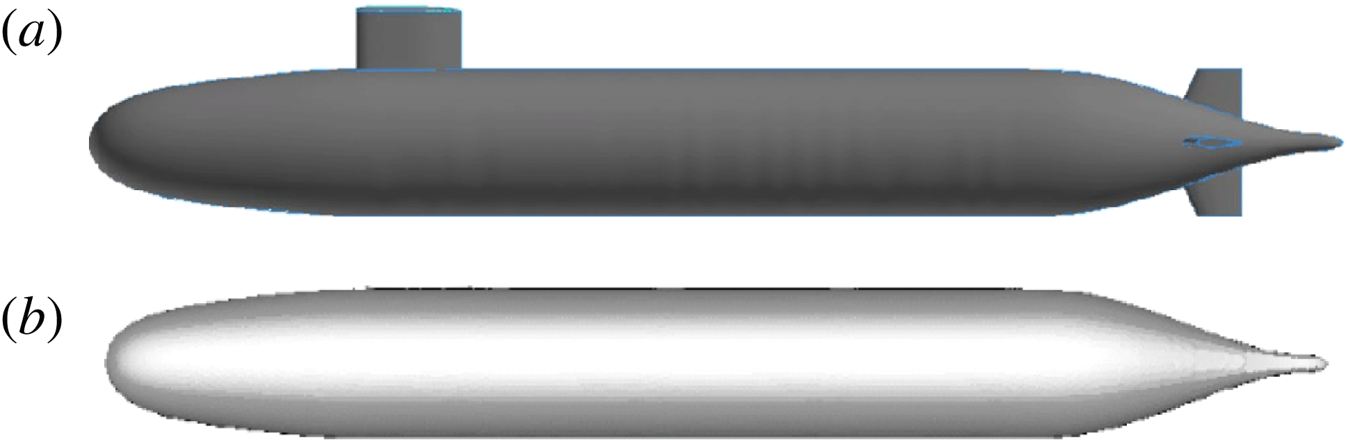
Geometry of fully appended hull, AFF8 (a) and bare hull, AFF1 (b) (Groves, Huang & Chang Reference Groves, Huang and Chang1989).

The geometry used in the present work is the generic submarine hull, DARPA SUBOFF without appendages (AFF1) (Groves et al.
Reference Groves, Huang and Chang1989). Figure 1 shows both fully appended hull (AFF8) and bare hull (AFF1) SUBOFF geometries. The SUBOFF geometry has been used in numerous past experiments and simulations. Huang et al. (Reference Huang, Liu, Grooves, Forlini, Blanton and Gowing1992) conducted SUBOFF experiments with and without appendages at
 $Re=1.2\times 10^{7}$
and reported pressure, skin friction and profiles of velocity statistics on the hull. Jiménez, Hultmark & Smits (Reference Jiménez, Hultmark and Smits2010b
) experimentally studied the evolution of the wake of the bare hull at
 $Re=1.1\times 10^{6}{-}6.7\times 10^{7}$
. Jiménez, Reynolds & Smits (Reference Jiménez, Reynolds and Smits2010c
) studied the effect of fins (appendages) on the intermediate wake of the fully appended SUBOFF. Traditionally, numerical simulations of such geometries solve Reynolds-averaged Navier–Stokes (RANS) equations to obtain time-averaged flow field behaviour. Yang & Löhner (Reference Yang and Löhner2003) accurately computed pressure and skin-friction coefficients using RANS equations. Kim, Rhee & Miller (Reference Kim, Rhee and Miller2013) performed RANS simulations for turning manoeuvre of SUBOFF. The capabilities of detached eddy simulation (DES) and LES to accurately predict flow over SUBOFF, both appended and unappended, are reviewed by Alin et al. (Reference Alin, Bensow, Fureby, Huuva and Svennberg2010). They showed that LES gives a better representation of the flow field, particularly for second-order statistics, compared to DES. There are numerous other computational studies employing the RANS, DES and delayed detached eddy simulation (DDES) techniques to study flow over SUBOFF (Vaz, Toxopeus & Holmes Reference Vaz, Toxopeus and Holmes2010; Chase & Carrica Reference Chase and Carrica2013; Chase, Michael & Carrica Reference Chase, Michael and Carrica2013). Simulations of complex flows of engineering importance using LES are gaining popularity in recent years due to the advent of computational facilities and the development of better numerical algorithms. Mahesh et al. (Reference Mahesh, Kumar, Gnanaskandan and Nitzkorski2015) reviewed the capability of LES to simulate complex flows relevant to marine applications.
Posa & Balaras (Reference Posa and Balaras2016) performed wall-resolved LES of flow over fully appended SUBOFF at
 $Re=1.2\times 10^{6}$
i.e. conditions similar to the experiments of Jiménez et al. (Reference Jiménez, Reynolds and Smits2010c
). Their study was focused on the effect of appendages and the interaction of the junction flows created by the appendages with the wake. The evolution of the wake was captured up to nine diameters downstream of the hull. The wake parameters were evaluated and compared to the measurements of Jiménez et al. (Reference Jiménez, Reynolds and Smits2010c
). It was found that the wake is strongly influenced by the appendages, and a bimodal behaviour for the turbulent stresses was observed due to flow separation on the stern portion of the hull causing the displacement of the maximum of the kinetic energy away from the wall, consistent with the reference experiments (Jiménez et al.
Reference Jiménez, Reynolds and Smits2010c
).
Note that the present work is substantially different from Posa & Balaras (Reference Posa and Balaras2016), both in terms of the hull geometry and the numerical method. The present simulations are based on the experiments of Jiménez et al. (Reference Jiménez, Hultmark and Smits2010b ), which are a different set of experiments conducted in the same tunnel and set-up for the hull geometry without stern appendages. Moreover, the numerical approach to solve the governing equations is entirely different. The present simulations use an unstructured body-fitted grid with a finite-volume approach (described in § 2.1) unlike Posa & Balaras (Reference Posa and Balaras2016), who used a cylindrical structured computational grid with a finite-difference approach where the boundary conditions on the wall are enforced using the direct-forcing immersed boundary method as the grid does not coincide with the wall (see Posa & Balaras Reference Posa and Balaras2016, for details).
The present work is focused on the flow over an axisymmetric hull, and its wake. There are two main challenges associated with studying turbulent wakes generated by streamlined bodies: the thin hull boundary layer and long wake development length. Computationally, this requires fine grid resolution for a long domain devoid of confinement effects to capture near-wall structures as well as wake evolution. Additionally, the numerical scheme should avoid unphysical dissipation of the velocity fluctuations, which keep getting smaller as the wake evolves away from the wake generator.
In the present work, wall-resolved LES of flow over a bare hull is performed at
 $Re=1.1\times 10^{6}$
, based on length of the hull and the free-stream velocity. Care has been taken to eliminate confinement effects and to capture essential flow features. The grid resolution and length of the simulated wake in the present work are significantly higher than most past works. The objectives of the present work are to evaluate the ability of LES to predict the flow over axisymmetric hull and to characterize the evolution of the axisymmetric wake of the hull. The paper is organized as follows. The set-up of the simulation including the numerical method, the computational grid and the boundary conditions, as well as grid convergence are discussed in § 2. Results along with a comparison to available data are described in § 3. Finally, the work is summarized in § 4.
2 Simulation details
2.1 Numerical method
In LES, large scales are resolved by the spatially filtered Navier–Stokes equations and the effect of small scales is modelled. The spatially filtered incompressible Navier–Stokes equations are:
 $$\begin{eqnarray}\left.\begin{array}{@{}c@{}}\displaystyle \frac{\unicode[STIX]{x2202}\overline{u}_{i}}{\unicode[STIX]{x2202}t}+\frac{\unicode[STIX]{x2202}}{\unicode[STIX]{x2202}x_{j}}(\overline{u}_{i}\overline{u}_{j})=-\frac{\unicode[STIX]{x2202}\overline{p}}{\unicode[STIX]{x2202}x_{i}}+\unicode[STIX]{x1D708}\frac{\unicode[STIX]{x2202}^{2}\overline{u}_{i}}{\unicode[STIX]{x2202}x_{j}\unicode[STIX]{x2202}x_{j}}-\frac{\unicode[STIX]{x2202}\unicode[STIX]{x1D70F}_{ij}}{\unicode[STIX]{x2202}x_{j}},\\ \displaystyle \frac{\unicode[STIX]{x2202}\overline{u}_{i}}{\unicode[STIX]{x2202}x_{i}}=0,\end{array}\right\}\end{eqnarray}$$
where
 $u_{i}$
is the velocity,
 $p$
is the pressure and
 $\unicode[STIX]{x1D708}$
is the kinematic viscosity. The overbar
 $\overline{(\cdot )}$
denotes spatial filtering and
 $\unicode[STIX]{x1D70F}_{ij}=\overline{u_{i}u_{j}}-\overline{u}_{i}\overline{u}_{j}$
is the sub-grid stress. The sub-grid stress is modelled using the dynamic Smagorinsky model (Germano et al.
Reference Germano, Piomelli, Moin and Cabot1991; Lilly Reference Lilly1992). The Lagrangian time scale is dynamically computed based on surrogate correlation of the Germano-identity error (Park & Mahesh Reference Park and Mahesh2009). This approach extended to unstructured grids has shown good performance for a variety of flows including plane channel flow, circular cylinder and flow past a marine propeller in crashback (Verma & Mahesh Reference Verma and Mahesh2012).
Equation (2.1) is solved using a numerical method developed by Mahesh, Constantinescu & Moin (Reference Mahesh, Constantinescu and Moin2004) for incompressible flows on unstructured grids. The algorithm is derived to be robust without numerical dissipation. It is a finite-volume method where the Cartesian velocities and pressure are stored at the centroids of the cells and the face normal velocities are stored independently at the centroids of the faces. A predictor–corrector approach is used. The predicted velocities at the control volume centroids are first obtained and then interpolated to obtain the face normal velocities. The predicted face normal velocity is projected so that the continuity equation in (2.1) is discretely satisfied. This yields a Poisson equation for pressure which is solved iteratively using a multigrid approach. The pressure field is used to update the Cartesian control volume velocities using a least-square formulation. Time advancement is performed using an implicit Crank–Nicholson scheme. The algorithm has been validated for a variety of problems over a range of Reynolds numbers (see Mahesh et al. Reference Mahesh, Constantinescu and Moin2004). Recently, Kumar & Mahesh (Reference Kumar and Mahesh2017) used this algorithm to accurately simulate complex propeller wakes.
2.2 Geometry, computational domain and boundary conditions
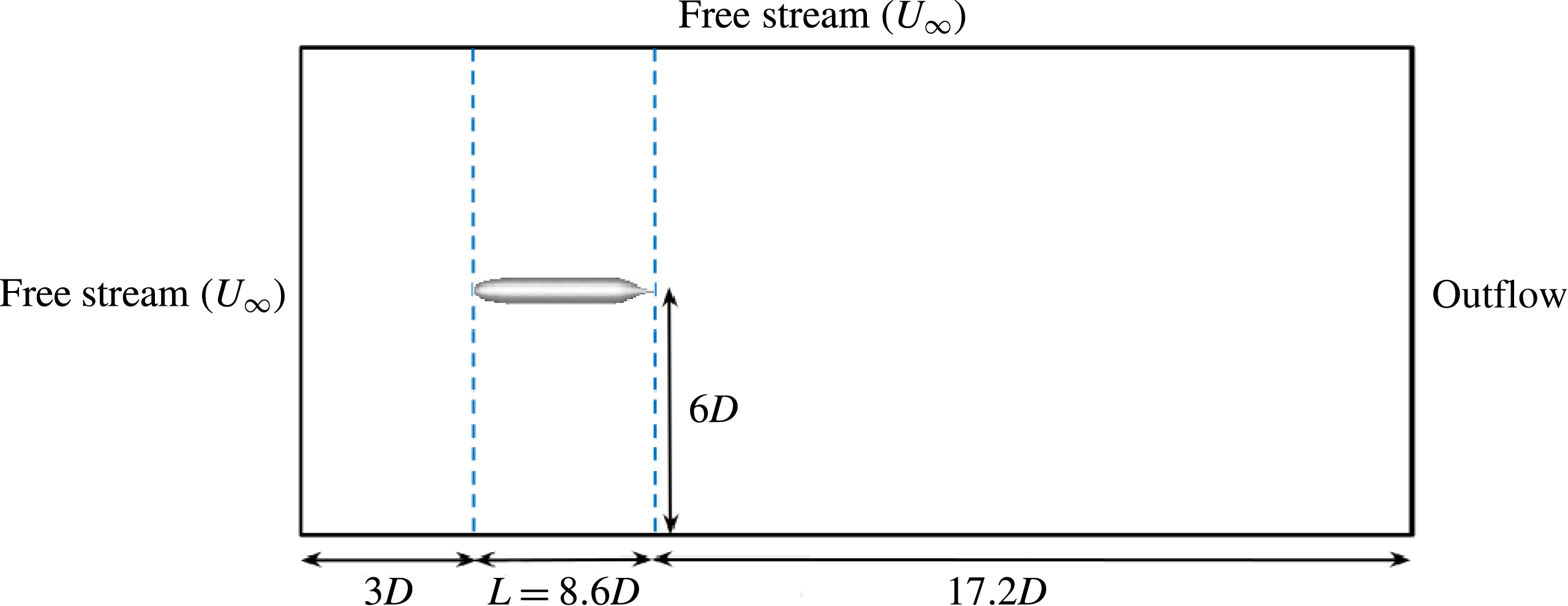
LES of flow over a bare hull (figure 1
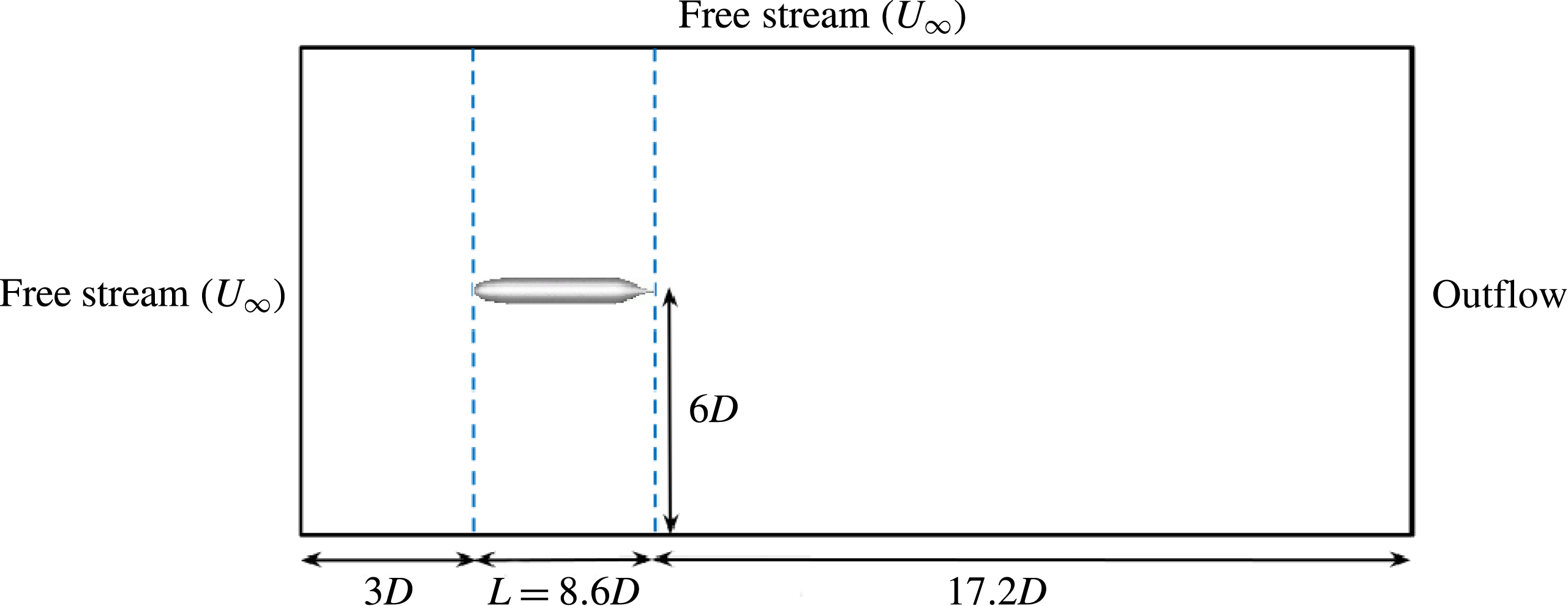
b) is performed using a cylindrical computational domain of length
 $28.8D$
and diameter
 $12D$
, where
 $D$
is the maximum diameter of the hull. The origin of the reference coordinate system is located at the nose of the hull. The inflow plane is located
 $3D$
upstream of the hull while the outflow is located
 $17.2D$
downstream of the stern. Note that the length of the hull is
 $L=8.6D$
. Preliminary simulations were used to estimate the size of the required computational domain and are discussed in § 2.3. The current computational domain is bigger than that used by Posa & Balaras (Reference Posa and Balaras2016) to simulate flow over fully appended SUBOFF at
 $Re=1.2\times 10^{6}$
.
The physical conditions of the present simulations are identical to those of the experiments conducted by Jiménez et al. (Reference Jiménez, Hultmark and Smits2010b
), with the difference that a semi-infinite sail was used as support in the experiments. The hull boundary layer in the simulations stays laminar without tripping. The hull boundary layer therefore is tripped at the same location (
 $x/D=0.75$
) as that of the experiment, by applying a steady wall-normal velocity perturbation. This lifts the boundary layer and mimics the presence of a trip wire. This method of tripping was tested in preliminary simulations, where a small steady wall-normal velocity over few cells quickly turned an axisymmetric laminar boundary layer turbulent.
The computations reported in the present work are performed on an unstructured grid consisting of approximately 608 million hexahedral control volumes partitioned over 8192 processors. The computational time step
 $tU/D=0.0006$
is used. The simulations are performed for over two flow-through times to discard transients and the results are sampled for another two flow-through times to compute converged statistics. Free-stream velocity boundary conditions are specified at the inflow and the lateral boundaries. Convective boundary conditions are prescribed at the outflow. No-slip boundary conditions are prescribed on the hull surface. A schematic of the computational domain and the boundary conditions is shown in figure 2.
The computational domain used for simulations of flow over the hull.
2.3 Grid convergence and sensitivity
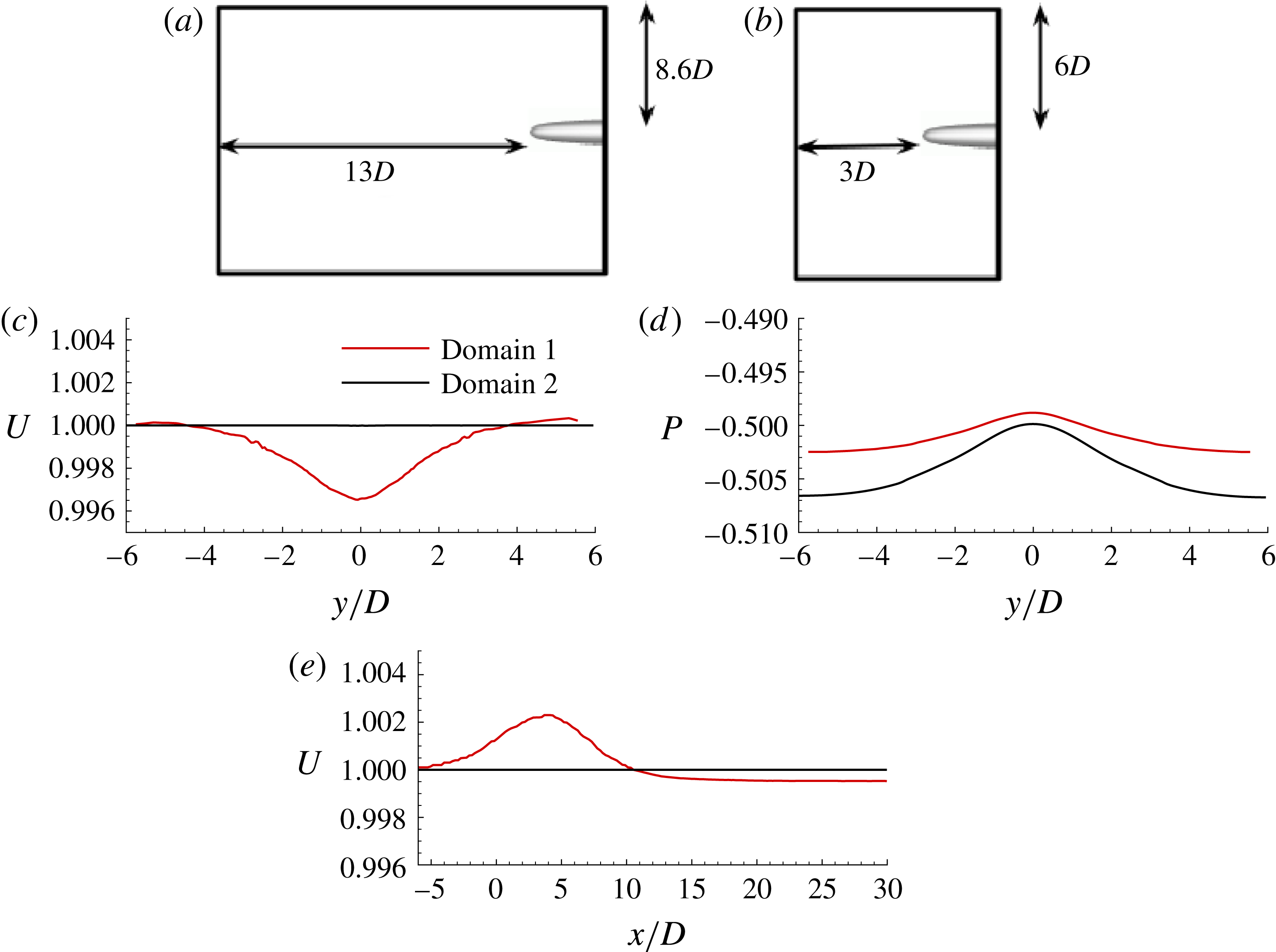
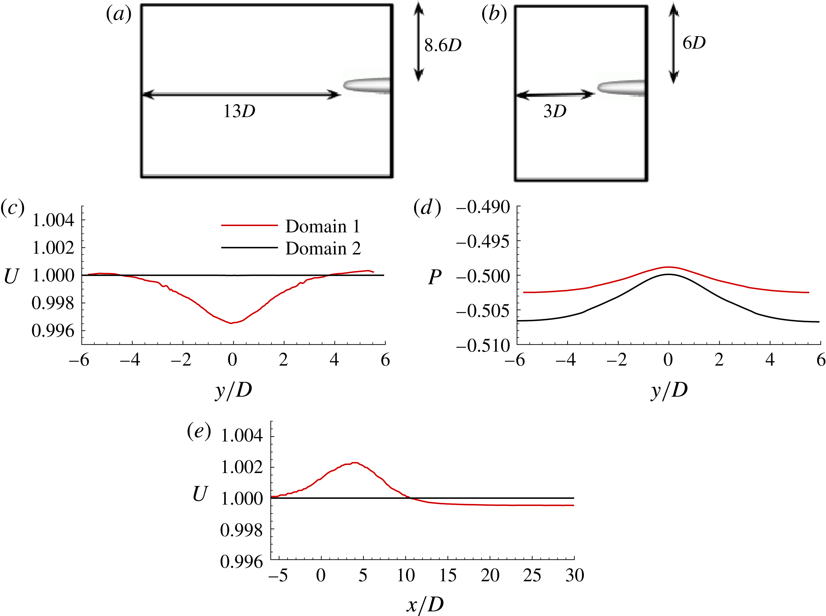
The size of the computational domain was chosen based on the results of preliminary simulations on a coarse grid. The preliminary simulations were performed on two domains (figure 3
a,b), domain 1 and 2, to assess confinement effects. Profiles of axial velocity and pressure are extracted and compared at
 $x/D=-3$
for both the domains in figures 3(c) and 3(d) respectively. The pressure at the stagnation point on the nose of the hull is used as reference pressure. Figure 3(e) shows the axial velocity profile at a radial distance of
 $6D$
for both of the domains. It can be concluded that choosing the inflow plane at
 $3D$
upstream of the hull and lateral boundary at a radial distance of
 $6D$
from the axis in the computational domain will have negligible confinement effects.
Domains 1 (a) and 2 (b) are used for confinement studies. Inflow confinement: instantaneous axial velocity,
 $U$
(c) and pressure difference from the stagnation (nose of hull),
 $P$
(d) are compared at
 $x/D=-3$
for the two domains. Radial confinement:
 $U$
(e) is compared at
 $y/D=6$
for the two domains. Domain 2 has negligible confinement.
The thin boundary layer on the hull and the turbulent axisymmetric wake need to be captured, which requires fine resolution. The computational grid used in the present work is clustered near the surface of the hull with a wall-normal spacing of
 $0.0003D$
and a growth ratio of 1.01 away from the wall. The near-wall streaks are responsible for the skin friction, and require fine azimuthal resolution. There are 1600 uniformly spaced cells in the azimuthal direction, yielding azimuthal resolution
 $a^{+}\unicode[STIX]{x0394}\unicode[STIX]{x1D703}=11$
, where
 $a$
is the radius of curvature and
 $a^{+}=au_{\unicode[STIX]{x1D70F}}/\unicode[STIX]{x1D708}$
, at a representative location on the mid-portion of the body. The streamwise (
 $x^{+}$
) and first wall-normal (
 $y^{+}$
) grid resolutions are less than 33 and 1 wall units respectively, over most of the hull where the flow is attached. Note that these grid spacings were estimated from a coarse LES simulation at the same
 $Re$
. This ensures adequate resolution at the mid-region of the hull.
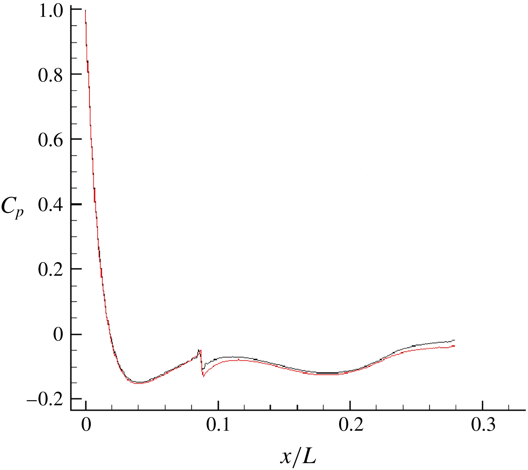
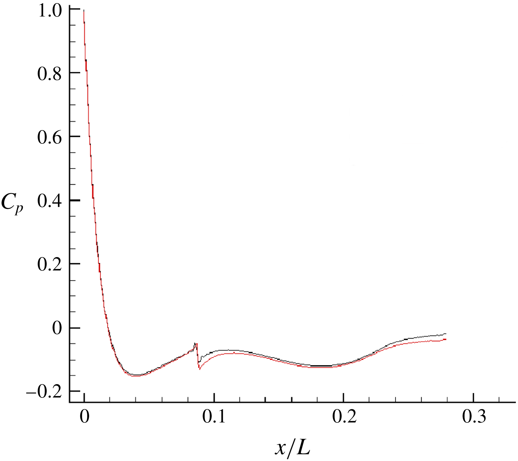
Grid convergence for
 $C_{p}$
on the bow region. A further four times refinement in the streamwise resolution (——, red) does not change the pressure drop appreciably compared to the grid resolution used in the present simulations (——, black) for the bow region.
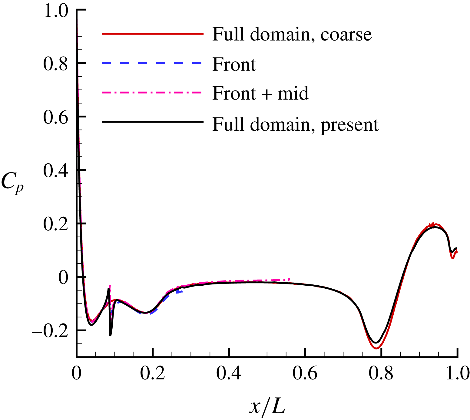
Next, the bow and the stern regions were assessed for grid convergence as they are crucial for ensuring a proper boundary layer and wake. The entire domain was split into different parts – bow, mid and stern regions and simulated individually, to ensure the correct solution, before merging them together for the final simulation.
The pressure and skin-friction coefficients are defined as:
 $$\begin{eqnarray}\displaystyle C_{p}=\frac{p-p_{\infty }}{0.5\unicode[STIX]{x1D70C}U_{\infty }^{2}}\quad \text{and}\quad C_{f}=\frac{\unicode[STIX]{x1D70F}_{w}}{0.5\unicode[STIX]{x1D70C}U_{\infty }^{2}}. & & \displaystyle\end{eqnarray}$$
The reference pressure (
 $p_{\infty }$
) is taken at the inflow near the radial boundary, and
 $\unicode[STIX]{x1D70F}_{w}$
is the shear stress at the wall. Different streamwise resolutions on the bow were tested to arrive at a grid resolution which ensures grid convergence in the pressure drop on the bow. A further refinement of the grid in the streamwise direction did not change the pressure drop on the bow appreciably, as shown in figure 4. Next, the grid convergence of
 $C_{p}$
is assessed on rest of the hull. Profiles of
 $C_{p}$
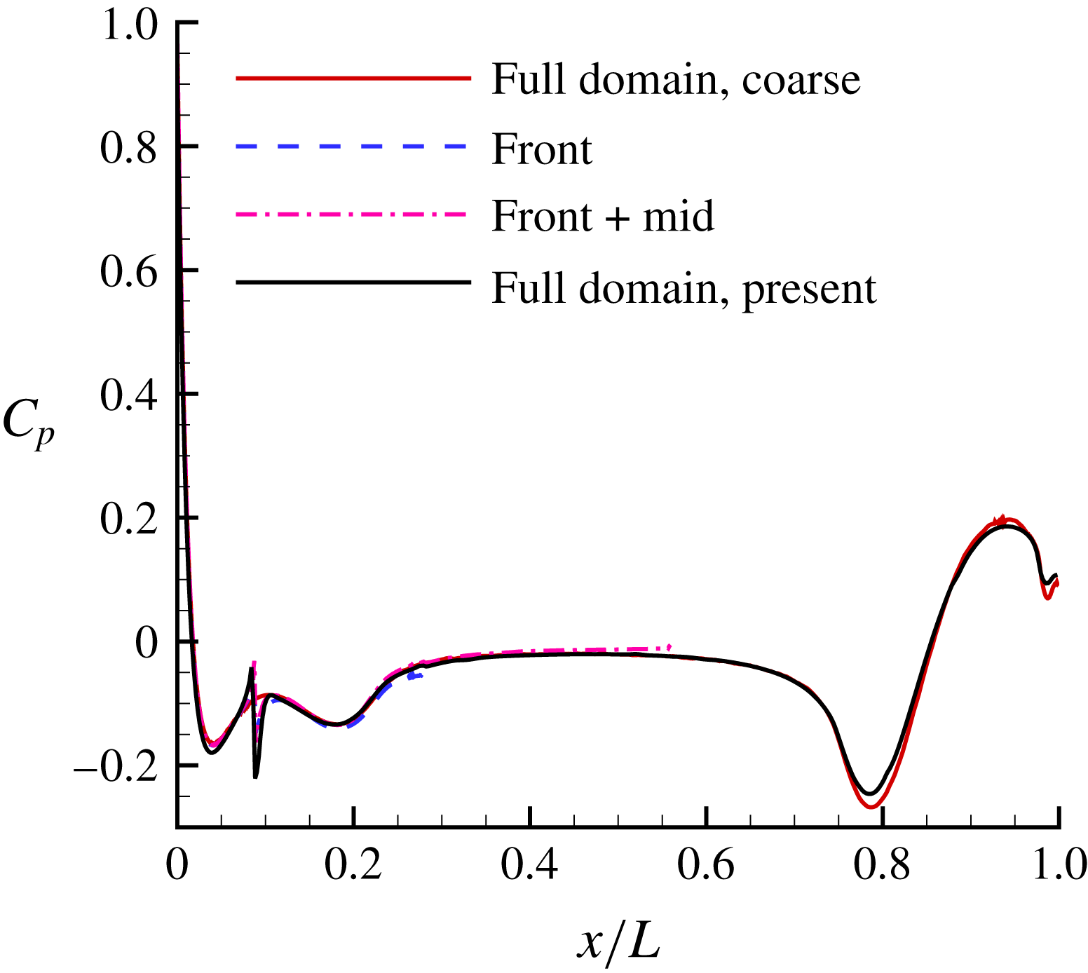
for the coarse grid used to estimate proper grid resolution, all the preliminary simulations of the individual parts and the final grid used in the present work are shown in figure 5. Note that
 $C_{p}$
converges on the relatively quickly compared to
 $C_{f}$
. Grid convergence of
 $C_{f}$
required further refinement on the stern, as discussed later in this section.
Grid convergence for
 $C_{p}$
. Results from all the preliminary simulations are compared to the final grid. Note that grids 1–3 give identical
 $C_{p}$
, hence only the grid 2 result is shown as the present result.
Grid convergence for drag forces. All of these grids are for full domain with identical bow and mid-regions. The grids only differ in the streamwise resolution on the stern (
 $x/L>0.56$
). The streamwise resolution (
 $\unicode[STIX]{x0394}x/L$
) is listed at
 $x/L=0.8$
on the hull.

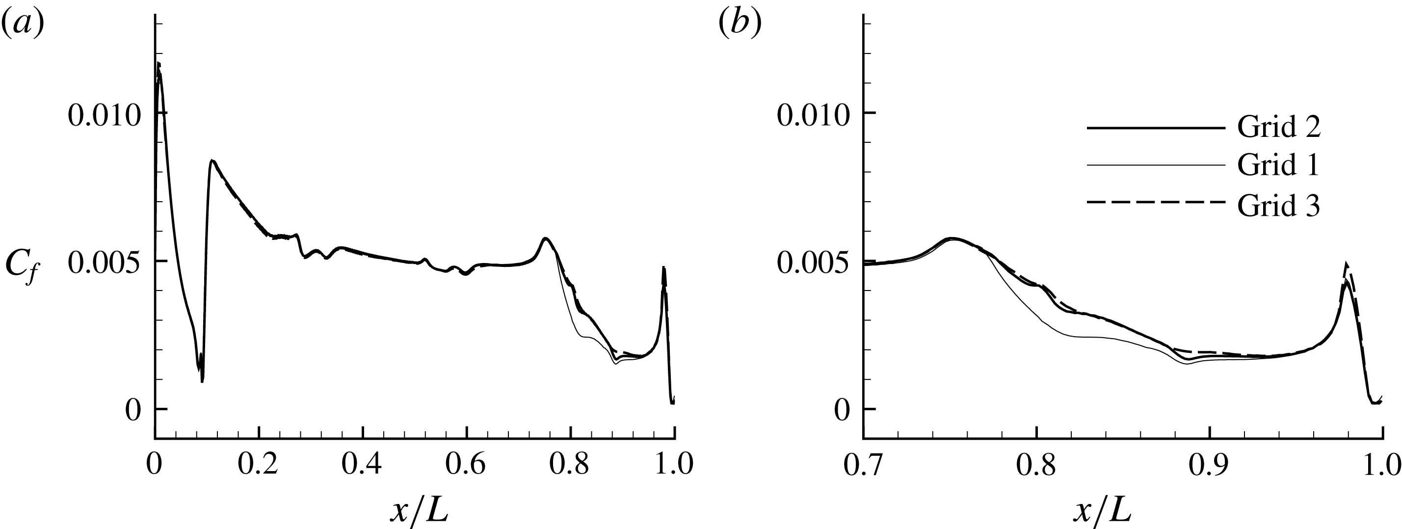
The wake of the hull is sensitive to properties of the stern boundary layer. The location of flow separation on the stern determines the wake width. Hence, it is important to ensure grid convergence and insensitivity to the flow field in the stern region. Simulations were performed for flow over the entire hull using three different streamwise resolutions at the stern region, as listed in table 1 for a location at
 $x/L=0.8$
on the hull. All of these grids (grids 1–3) have an identical front and mid-portion. Figure 6(a,b) shows the evolution of
 $C_{f}$
on the hull along with a zoomed-in view of the stern region. The change in
 $C_{f}$
is insignificant going from grid 2 to grid 3. The drag force contribution from both viscous and pressure forces are listed in table 1. There is no difference in the viscous force between grid 2 and grid 3, which confirms the grid convergence of
 $C_{f}$
. On the other hand, the pressure force shows a small (
 ${\sim}3\,\%$
) difference between grid 2 and grid 3. Since, the viscous force contributes most of the overall drag force, the difference in the overall drag force between grid 2 and grid 3 is negligible (
 ${\sim}0.5\,\%$
). The momentum deficit in the wake of the hull depends on the overall drag. Hence, the results reported here are from grid 2, which can be considered grid converged.
Grid convergence for
 $C_{f}$
on the hull. Grids 1–3 only differ in the streamwise resolution on the stern (
 $x/L>0.56$
), with grid 1 being the coarsest and grid 3 being the finest. The results from grid 2 are presented in this work.

2.4 Forces on the body
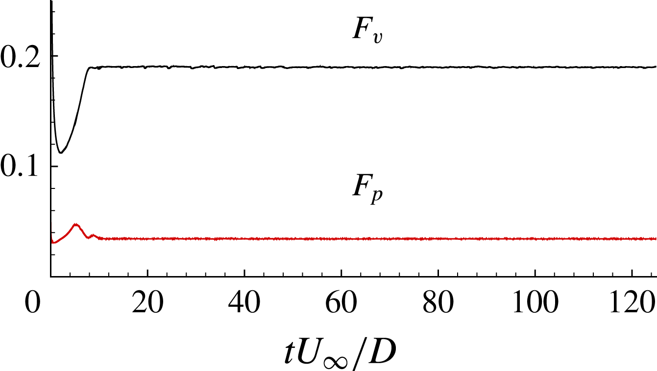
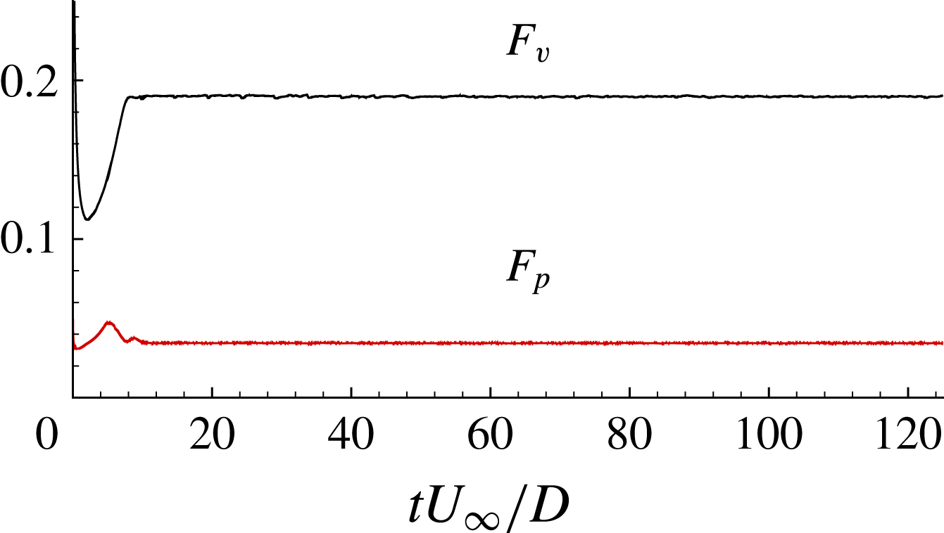
Figure 7 shows the time evolution of the overall pressure and viscous forces on the hull in the axial direction. These forces together yield the drag. As expected, most of the drag comes from viscous forces as the flow is largely attached. Note that the initial transients last for a small fraction of the flow-through time. In the simulation domain, one flow-through time
 $tU_{\infty }/D=28.8$
. The overall drag coefficient
 $$\begin{eqnarray}\displaystyle C_{D}=\frac{F}{0.5\unicode[STIX]{x1D70C}U_{\infty }^{2}S}, & & \displaystyle\end{eqnarray}$$
where
 $F$
is the drag force and
 $S=0.25\unicode[STIX]{x03C0}D^{2}$
is the projected area. The value of
 $C_{D}$
from LES is
 $0.204$
.
The time evolution of the drag force contribution from pressure (
 $F_{p}$
) and viscous forces (
 $F_{v}$
) on the hull. Note that one flow-through time is
 $tU_{\infty }/D=28.8$
.
3 Results
3.1 Overview of the flow field
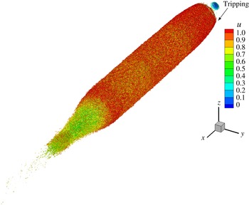
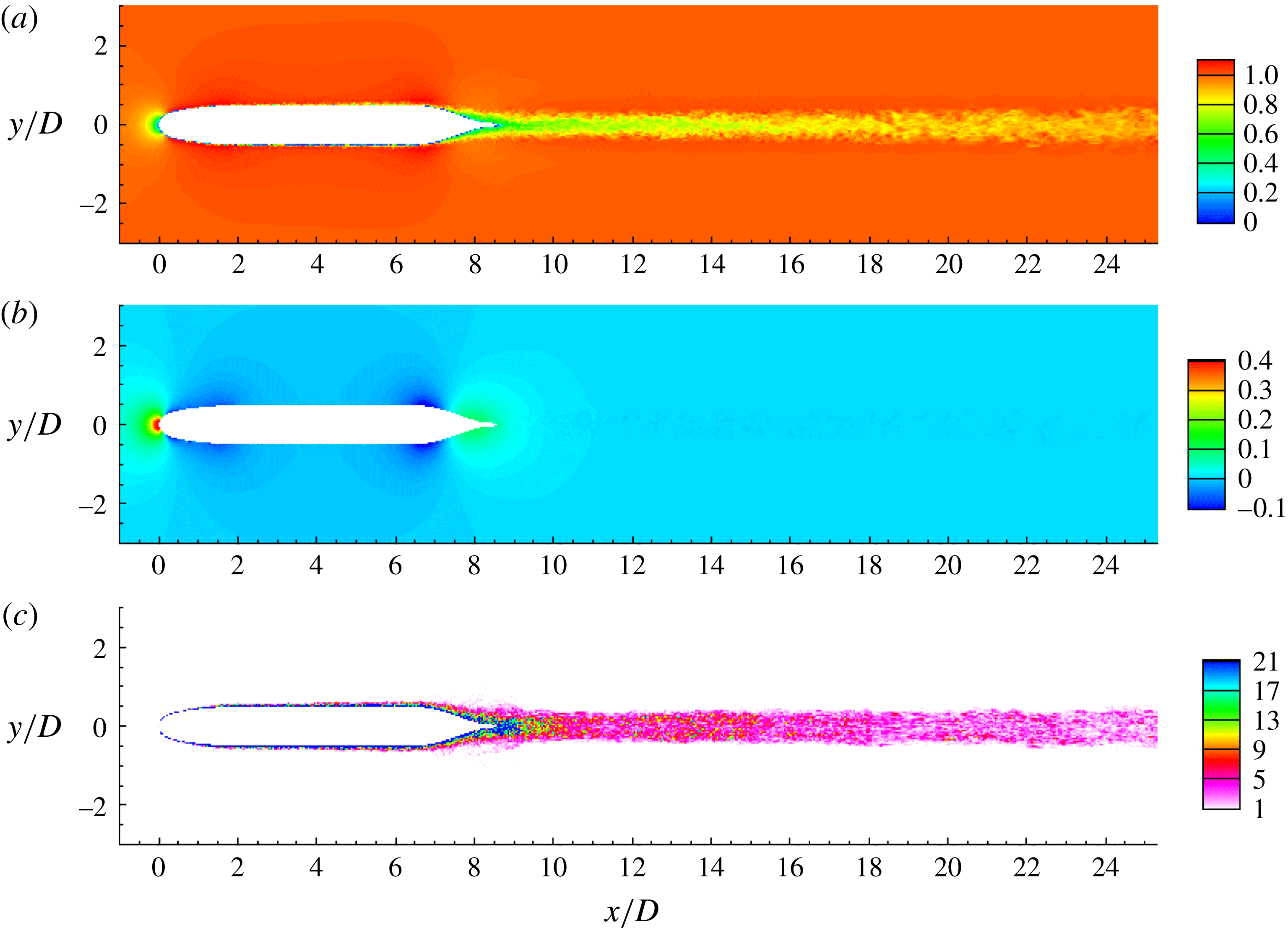
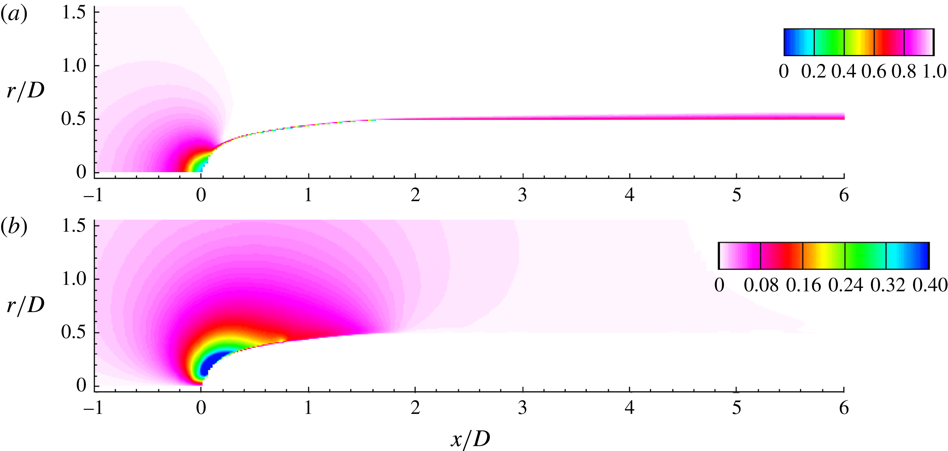
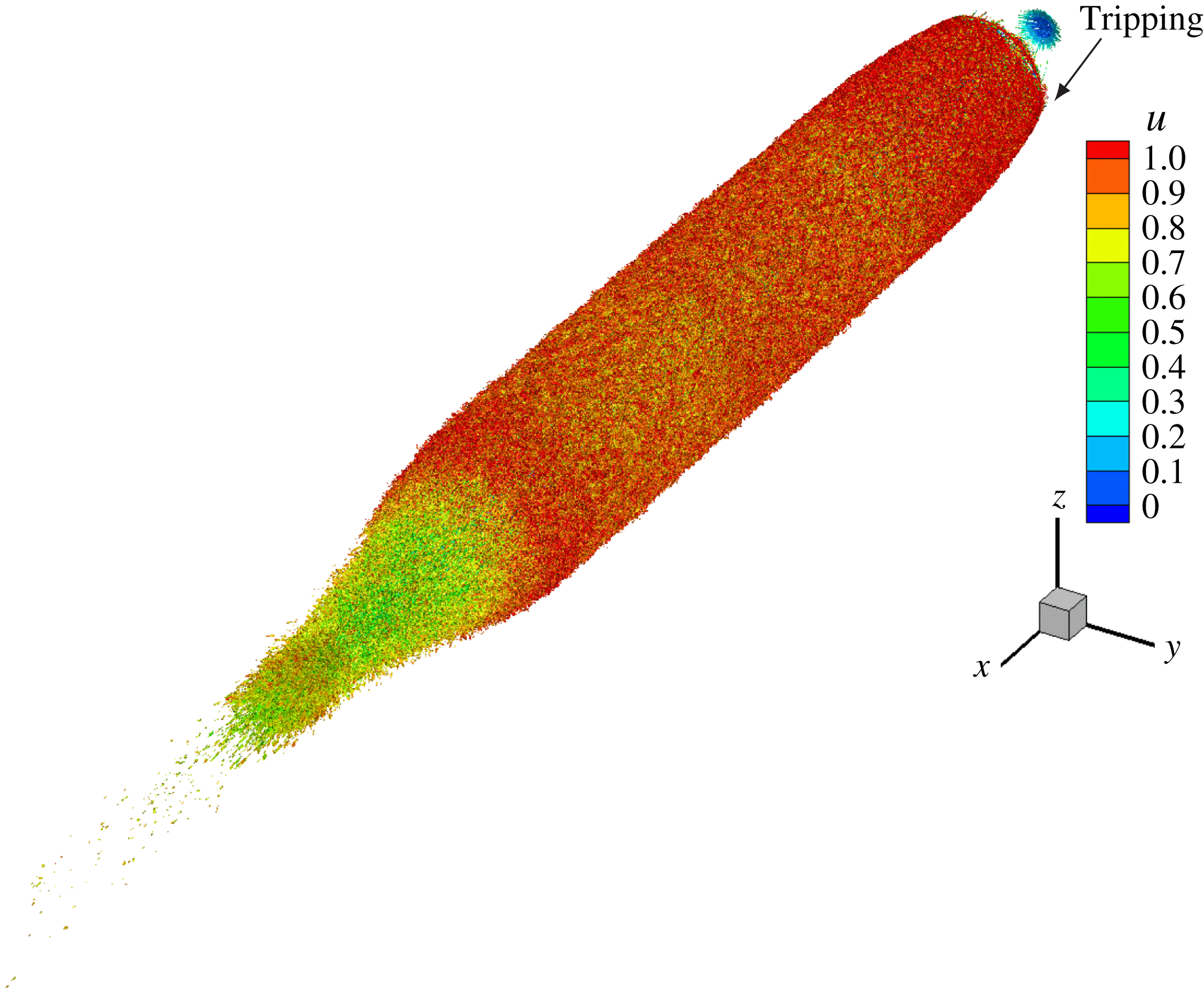
The instantaneous near-wall flow structures are visualized in figure 8 using isocontours of Q-criterion (Hunt, Wray & Moin Reference Hunt, Wray and Moin1988) coloured by axial velocity. The rapid transition following tripping is evident, and the near-wall flow structures appear to be adequately captured. Contours of instantaneous axial velocity, pressure and vorticity magnitude are shown in figure 9. Note that the flow is attached over the entire hull except the stern, as expected for a streamlined geometry. The flow accelerates on the bow due to favourable pressure gradient, quickly turns turbulent and evolves downstream on the mid-portion on the hull, which is a zero-pressure-gradient region. The axisymmetric turbulent boundary layer (TBL) eventually separates on the stern to form the wake. The pressure gradient is negligible in the wake region away from the stern. The slow radial spreading of the wake with streamwise distance downstream of the hull is also noticeable. The contour plot of vorticity magnitude shows the regions of intense turbulent activity, which are mainly the hull boundary layer and the wake. The magnitude of the vorticity decreases, moving downstream in the wake.
The near-wall flow structures on the hull are visualized using isocontour of instantaneous Q-criterion (Hunt et al. Reference Hunt, Wray and Moin1988) coloured by axial velocity. The boundary layer is tripped at the same location as the experiments of Jiménez et al. (Reference Jiménez, Hultmark and Smits2010b ).
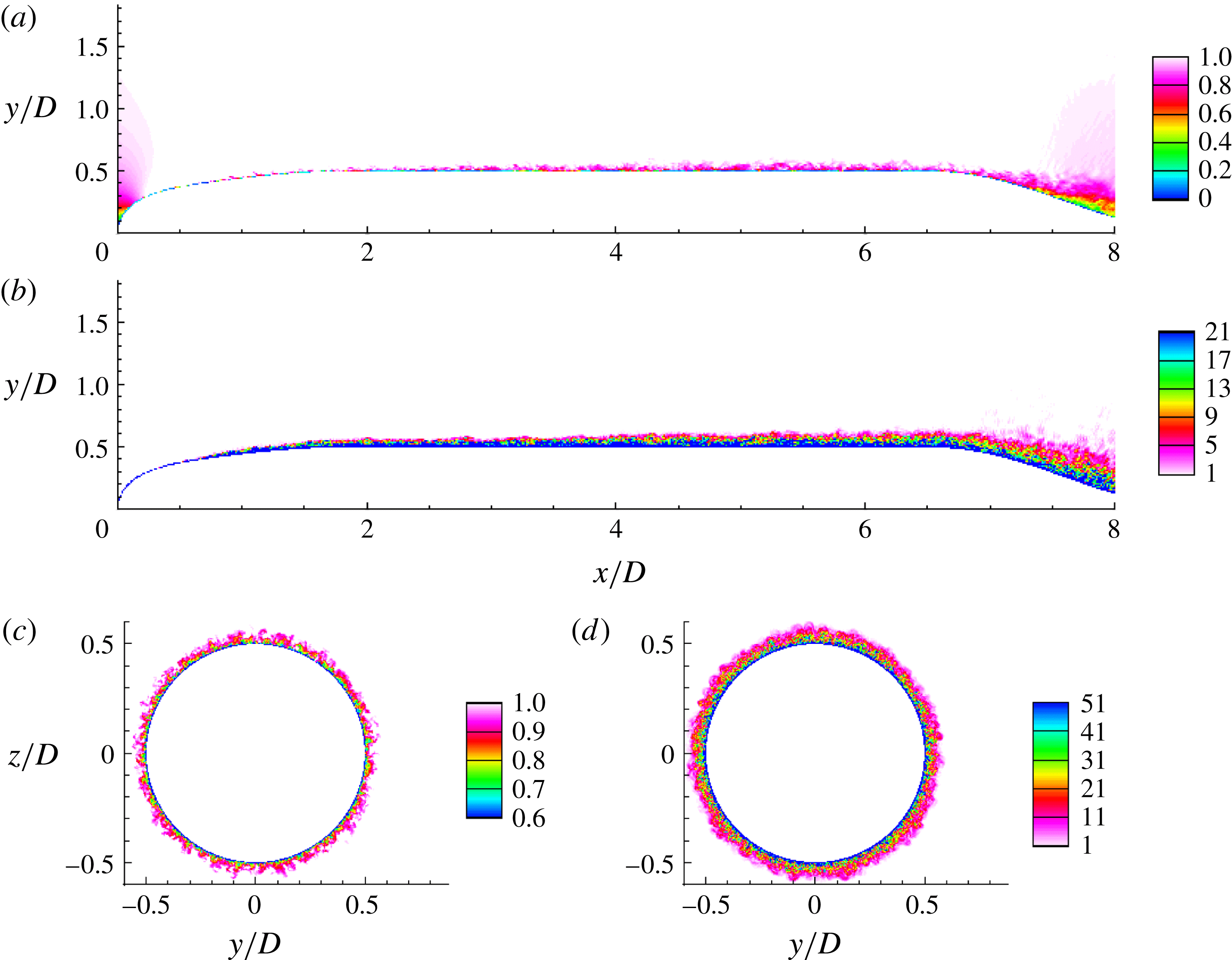
A closer view of the hull boundary layer is shown in figure 10. The effect of tripping and subsequent growth of the hull boundary layer is evident. The thickening of the hull boundary layer due to adverse pressure gradient on the stern can be observed, which eventually leads to flow separation and wake formation. Contours of axial velocity and vorticity magnitudes at transverse planes are shown in figure 10(c,d) at streamwise location
 $x/L=0.42$
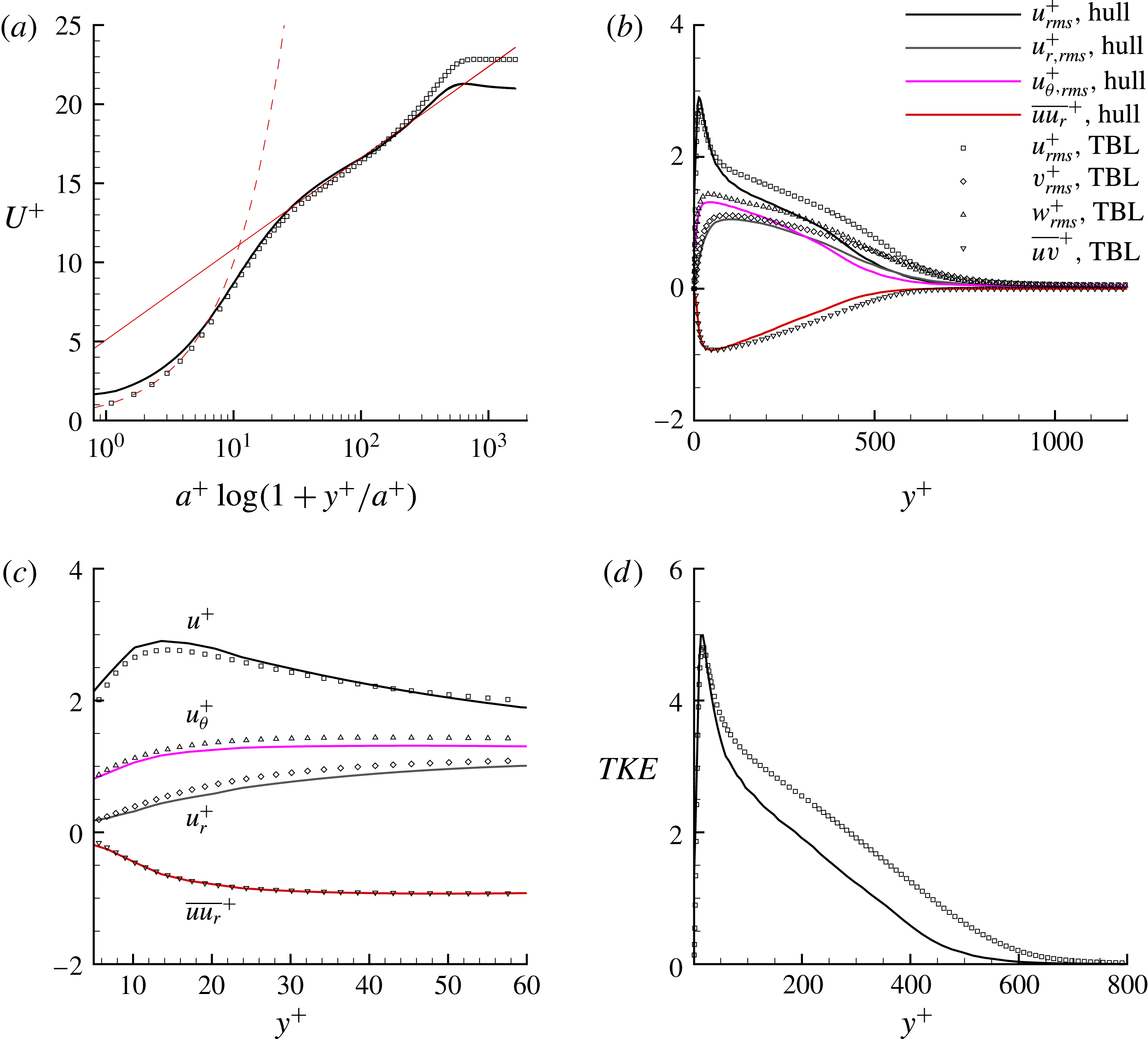
. The azimuthal resolution appears to capture the hull boundary layer adequately close to the wall. At this location, the profiles of first- and second-order velocity statistics are shown in figure 11. The direct numerical simulation (DNS) results of a planar TBL at
 $Re_{\unicode[STIX]{x1D703}}=1551$
from Jiménez et al. (Reference Jiménez, Hoyas, Simens and Mizuno2010a
) are also shown for comparison. Although the boundary layer thickness is similar (
 $\unicode[STIX]{x1D6FF}^{+}\sim 900$
), the friction velocity (
 $u_{\unicode[STIX]{x1D70F}}$
) for the hull boundary layer is higher, which makes
 $U^{+}$
smaller compared to the planar TBL value at similar
 $Re_{\unicode[STIX]{x1D703}}$
. This is due to the effect of transverse curvature of the hull on the axisymmetric TBL, as observed in past experiments and reviewed by Lueptow (Reference Lueptow1990).
Recently, Kumar & Mahesh (Reference Kumar and Mahesh2018) obtained a relation between
 $C_{f}$
and the boundary layer integral quantities for a generic axisymmetric boundary layer evolving under pressure gradients as
 $$\begin{eqnarray}C_{f}=\frac{\displaystyle 2\left(1+\frac{\unicode[STIX]{x1D703}}{a}\right)\frac{\unicode[STIX]{x1D6FF}^{\ast }}{\unicode[STIX]{x1D6FF}}\frac{\text{d}\unicode[STIX]{x1D6FF}}{\text{d}x}}{\displaystyle H+\unicode[STIX]{x1D6FD}_{RC}\biggl[2+H\biggl(1+\frac{\unicode[STIX]{x1D6FF}^{\ast }}{2a}+\frac{\unicode[STIX]{x1D703}^{2}}{a\unicode[STIX]{x1D6FF}^{\ast }}\biggr)\biggr]},\end{eqnarray}$$
where,
 $\unicode[STIX]{x1D6FF}^{\ast }$
and
 $\unicode[STIX]{x1D703}$
are the displacement thickness and the momentum thickness of the boundary layer respectively (Luxton, Bull & Rajagopalan Reference Luxton, Bull and Rajagopalan1984),
 $H=\unicode[STIX]{x1D6FF}^{\ast }/\unicode[STIX]{x1D703}$
is the shape factor and
 $\unicode[STIX]{x1D6FD}_{RC}$
is the Rotta–Clauser pressure-gradient parameter (Rotta Reference Rotta1953; Clauser Reference Clauser1954) defined as,
 $$\begin{eqnarray}\displaystyle \unicode[STIX]{x1D6FD}_{RC}=\frac{\unicode[STIX]{x1D6FF}^{\ast }}{u_{\unicode[STIX]{x1D70F}}^{2}}\frac{1}{\unicode[STIX]{x1D70C}}\frac{\text{d}p}{\text{d}x}=-\frac{\unicode[STIX]{x1D6FF}^{\ast }}{u_{\unicode[STIX]{x1D70F}}^{2}}U_{e}\frac{\text{d}U_{e}}{\text{d}x}. & & \displaystyle\end{eqnarray}$$
It was also shown that for identical boundary layer parameters (
 $\unicode[STIX]{x1D6FF}$
,
 $\unicode[STIX]{x1D6FF}^{\ast }$
,
 $\unicode[STIX]{x1D703}$
,
 $\text{d}\unicode[STIX]{x1D6FF}/\text{d}x$
), the presence of transverse curvature always increases
 $C_{f}$
if
 $\unicode[STIX]{x1D6FD}_{RC}\geqslant 0$
. This explains the present observation of higher
 $C_{f}$
compared to a planar TBL at similar conditions.
The instantaneous flow field: axial velocity (a), pressure (b) and vorticity magnitude (c) in the
 $xy$
plane.

The hull boundary layer: instantaneous axial velocity (a,c) and vorticity magnitude (b,d) in the
 $xy$
(a,b) and
 $yz$
(c,d) planes. The
 $yz$
plane is extracted at
 $x/L=0.42$
(i.e.
 $x/D=3.6$
).

Radial (
 $u_{r}$
) and azimuthal (
 $u_{\unicode[STIX]{x1D703}}$
) velocity fluctuations are plotted for the hull boundary layer and compared to wall-normal (
 $v$
) and spanwise (
 $w$
) velocity fluctuations for a planar TBL. All the quantities are normalized using
 $u_{\unicode[STIX]{x1D70F}}$
. A closer view of the velocity fluctuations near the wall is shown in figure 11(c). In general, the axisymmetric TBL shows a similar trend to a planar TBL. However, the rapid decay in fluctuations away from the wall as compared to a planar TBL can be clearly observed. Closer to the wall (see figure 11
c), the second-order velocity statistics show good agreement with the planar TBL. The turbulent kinetic energy (TKE) profile of the axisymmetric TBL on the hull is compared to that of the planar TBL in figure 11(d). The TKE profile of the axisymmetric TBL decays faster than that of the planar TBL. Note that the curvature parameter,
 $\unicode[STIX]{x1D6FF}/a\approx 0.3$
at this location. It appears that curvature significantly affects the TKE in the log layer. Note the smaller value of Reynolds stress in the log region as well.
Statistics in wall units for hull boundary layer at
 $x/L=0.42$
on the hull: mean axial velocity (a), and root mean square (r.m.s.) of velocity fluctuations (
 $u_{rms}^{+}$
,
 $u_{r,rms}^{+}$
,
 $u_{\unicode[STIX]{x1D703},rms}^{+}$
) and Reynolds stress (
 $\overline{uv_{r}}^{+}$
) (b). Symbols show DNS of a planar TBL at
 $Re_{\unicode[STIX]{x1D703}}=1551$
(Jiménez et al.
Reference Jiménez, Hoyas, Simens and Mizuno2010a
). Zoomed-in view of the profiles of velocity fluctuations near peaks (c) and turbulent kinetic energy profile (d) are also shown. Here
 $a^{+}$
is the radius of the hull in wall units.

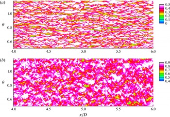
Cylindrical slices parallel to the hull surface are extracted at two radial locations,
 $r=0.836$
and
 $0.862$
, which correspond to
 $y^{+}=10$
and
 $110$
from the surface respectively, as shown in figure 12. The streaky flow structures in the buffer layer which are source of skin friction (Kline et al.
Reference Kline, Reynolds, Schraub and Runstadler1967), can be observed in figure 12(a) as marked by lower axial velocity. No such structures are observed in the logarithmic layer.
The hull boundary layer: wall-parallel cylindrical surfaces at a radial distance
 $r=0.836$
(a) and
 $r=0.862$
(b) from the axis. This corresponds to approximate
 $y^{+}=10$
and
 $110$
respectively away from the hull surface. Instantaneous axial velocity is shown on the mid-hull in the buffer and log region of the hull boundary layer.

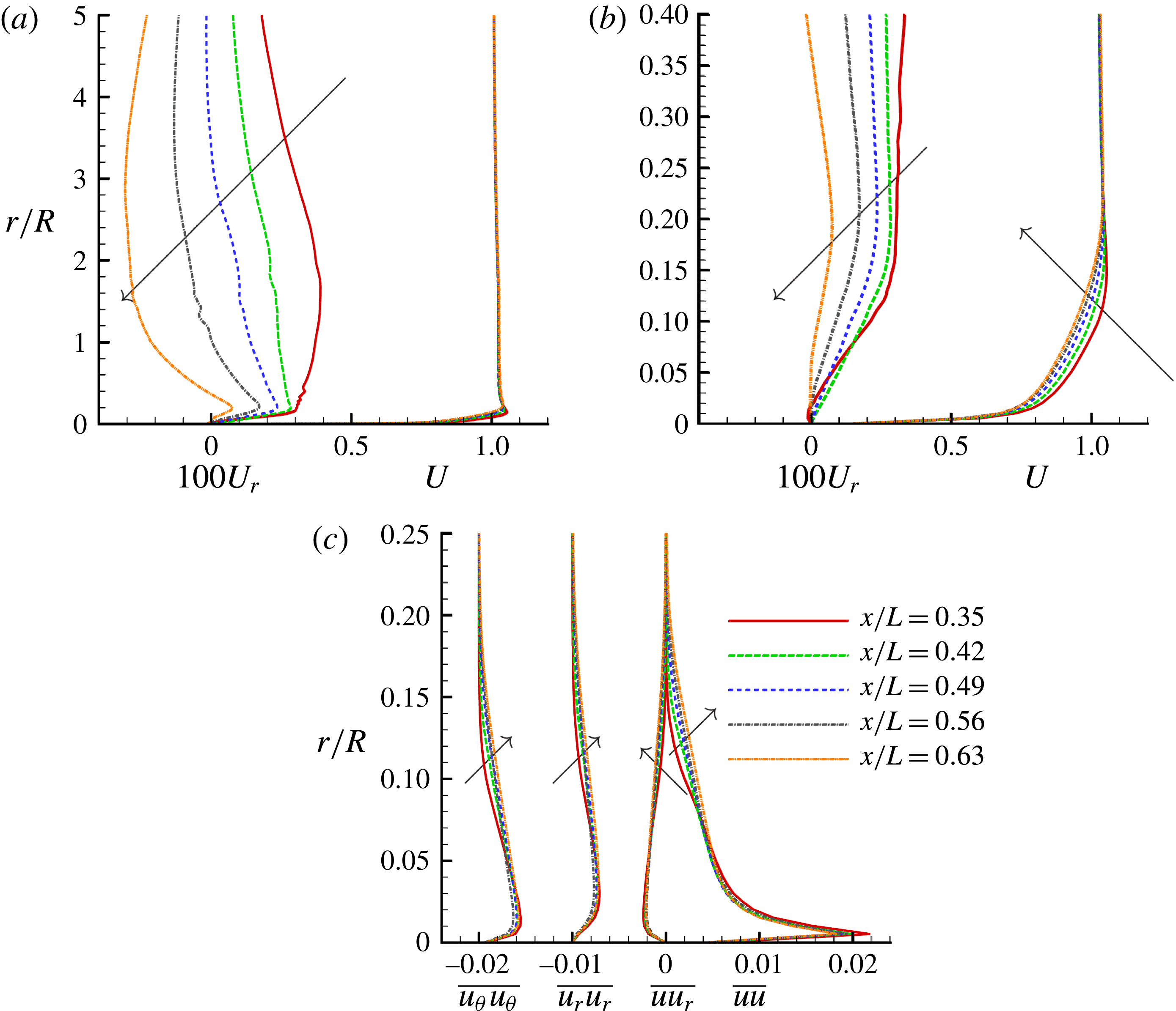
The streamwise growth of the hull boundary layer is examined using profiles of mean velocities, turbulent intensities and Reynolds stress at multiple locations on the hull (
 $0.35\leqslant x/L\leqslant 0.63$
) in figure 13. Figure 13(a) focuses on the flow outside the boundary layer. The value of
 $U_{r}$
varies very slowly outside the boundary layer. The first (
 $x/L=0.35$
) and last (
 $x/L=0.63$
) locations show relatively large variation in
 $U_{r}$
outside the boundary layer. In particular, the first location has increasing
 $U_{r}$
whereas, the opposite is observed at the last location. This behaviour of
 $U_{r}$
is due to a small favourable pressure gradient at the first and a small adverse pressure gradient at the last location, respectively. The spatial growth of the boundary layer thickness is clearly evident (figure 13
b,c).
The evolution of hull boundary layer: radial profiles of
 $U$
and
 $U_{r}$
(a) along with their close ups near the hull (b) are shown along with
 $\overline{uu}$
,
 $\overline{u_{r}u_{r}}$
,
 $\overline{u_{\unicode[STIX]{x1D703}}u_{\unicode[STIX]{x1D703}}}$
and
 $\overline{u_{r}u_{r}}$
at various locations on the hull from
 $x/L=0.35$
to
 $0.63$
(c). Note that the profiles of
 $\overline{u_{r}u_{r}}$
and
 $\overline{u_{\unicode[STIX]{x1D703}}u_{\unicode[STIX]{x1D703}}}$
are shifted to left by 0.01 and 0.02 units respectively for clarity. Arrows show the direction of increasing
 $x$
.

3.2 Comparison to experiments
The LES results of the present work are compared to the experiments of Huang et al. (Reference Huang, Liu, Grooves, Forlini, Blanton and Gowing1992) and Jiménez et al. (Reference Jiménez, Hultmark and Smits2010b
). Huang et al. (Reference Huang, Liu, Grooves, Forlini, Blanton and Gowing1992) conducted experiments of flow over bare hull and reported
 $C_{p}$
and
 $C_{f}$
on the hull at
 $Re=1.2\times 10^{7}$
. These measurements were made on a bare hull model identical to the present work and the model was supported by two thin NACA0015 struts (see Huang et al. (Reference Huang, Liu, Grooves, Forlini, Blanton and Gowing1992) for details), which had minimal effect on the flow field. Huang et al. (Reference Huang, Liu, Grooves, Forlini, Blanton and Gowing1992) reported measurement uncertainty of
 $\pm 0.015$
and
 $\pm 0.0002$
for
 $C_{p}$
and
 $C_{f}$
respectively and the measured
 $C_{p}$
was corrected for error due to confinement effects.
Jiménez et al. (Reference Jiménez, Hultmark and Smits2010b
) conducted experiments on the bare hull at
 $Re=1.1\times 10^{6}{-}6.7\times 10^{7}$
. The focus of their study was the evolution of the intermediate wake, and the wake profiles for the first- and second-order statistics at various streamwise locations downstream from the stern were reported. They did not report the evolution of
 $C_{f}$
, or the velocity profiles on the hull. The bare hull in their experiments had a semi-infinite sail, which acted as support. They report an overall blockage of
 $5.7\,\%$
in their wind tunnel due to the hull and the semi-infinite sail. The reported
 $C_{p}$
was not corrected for confinement and blockage effects.
The
 $C_{p}$
measured by Jiménez et al. (Reference Jiménez, Hultmark and Smits2010b
) on the hull did not match with the earlier experiments of Huang et al. (Reference Huang, Liu, Grooves, Forlini, Blanton and Gowing1992), which they attributed to a difference in reference pressure. The
 $C_{p}$
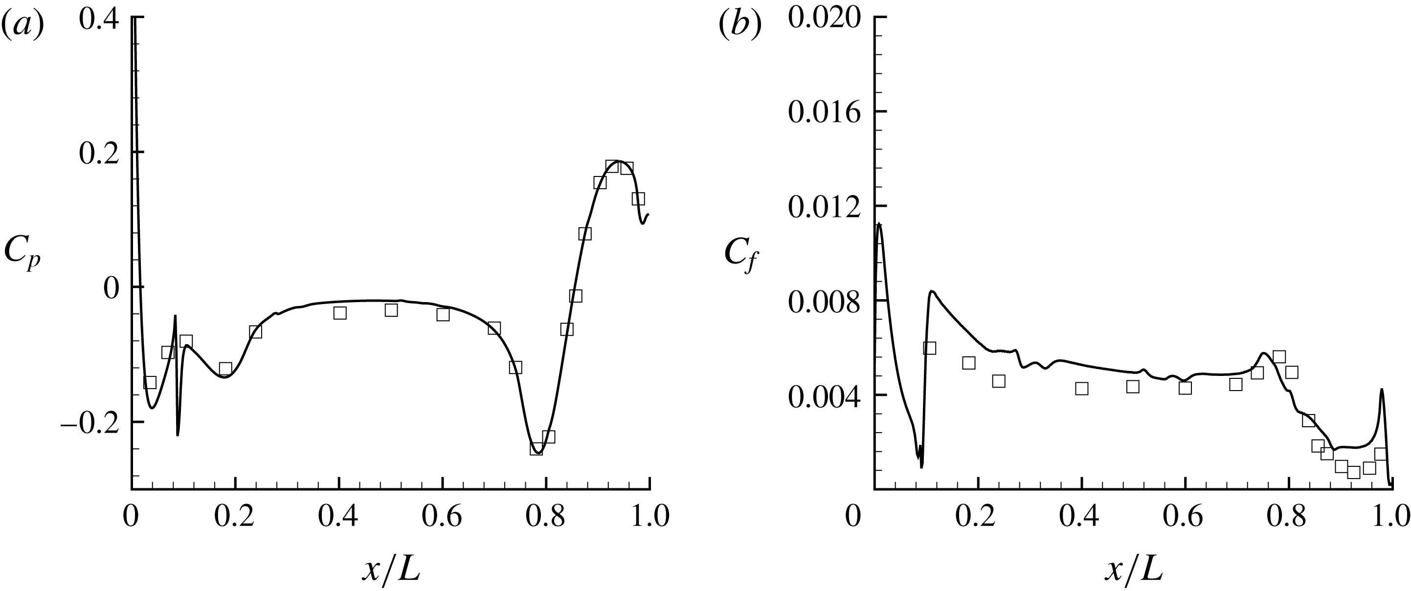
obtained from the simulations is compared to the experiments of Huang et al. (Reference Huang, Liu, Grooves, Forlini, Blanton and Gowing1992) in figure 14(a) showing good agreement, consistent with the results of Posa & Balaras (Reference Posa and Balaras2016). In rest of this section, LES results are compared to the available experiments.
 $C_{p}$
and
 $C_{f}$
on the hull, and the profiles of velocity and pressure statistics on the stern are compared to Huang et al. (Reference Huang, Liu, Grooves, Forlini, Blanton and Gowing1992). The wake profiles for mean and variance of axial velocity are compared to the data reported by Jiménez et al. (Reference Jiménez, Hultmark and Smits2010b
).
Note that the experiments of Huang et al. (Reference Huang, Liu, Grooves, Forlini, Blanton and Gowing1992) were conducted at
 $Re=1.2\times 10^{7}$
, whereas the simulations reported in the present work have
 $Re=1.1\times 10^{6}$
.
 $C_{p}$
is insensitive to
 $Re$
for high
 $Re$
attached flows but
 $C_{f}$
depends on
 $Re$
. Hence,
 $C_{f}$
values of the experiments are scaled to the
 $Re$
of the simulations using
 $C_{f}\sim Re^{-0.2}$
which applies to zero-pressure-gradient boundary layers. Note that the spike visible in the plots at
 $x/D=0.75$
is due to tripping. The difference between the
 $C_{f}$
from LES and the experiments at the bow and the stern regions is due to the inapplicability of the scaling law in regions of pressure gradient. The difference in
 $C_{f}$
on the bow region could also be due to the difference in tripping in the experiments. Overall, the LES results show good agreement with the experiments (figure 14
b).
 $C_{p}$
(a) and
 $C_{f}$
(b) on the hull. Symbols are measurements from the experiments of Huang et al. (Reference Huang, Liu, Grooves, Forlini, Blanton and Gowing1992) at
 $Re=1.2\times 10^{7}$
.
 $C_{f}$
from the experiments are scaled to the
 $Re$
of the simulations using scaling law,
 $C_{f}\sim Re^{-0.2}$
.

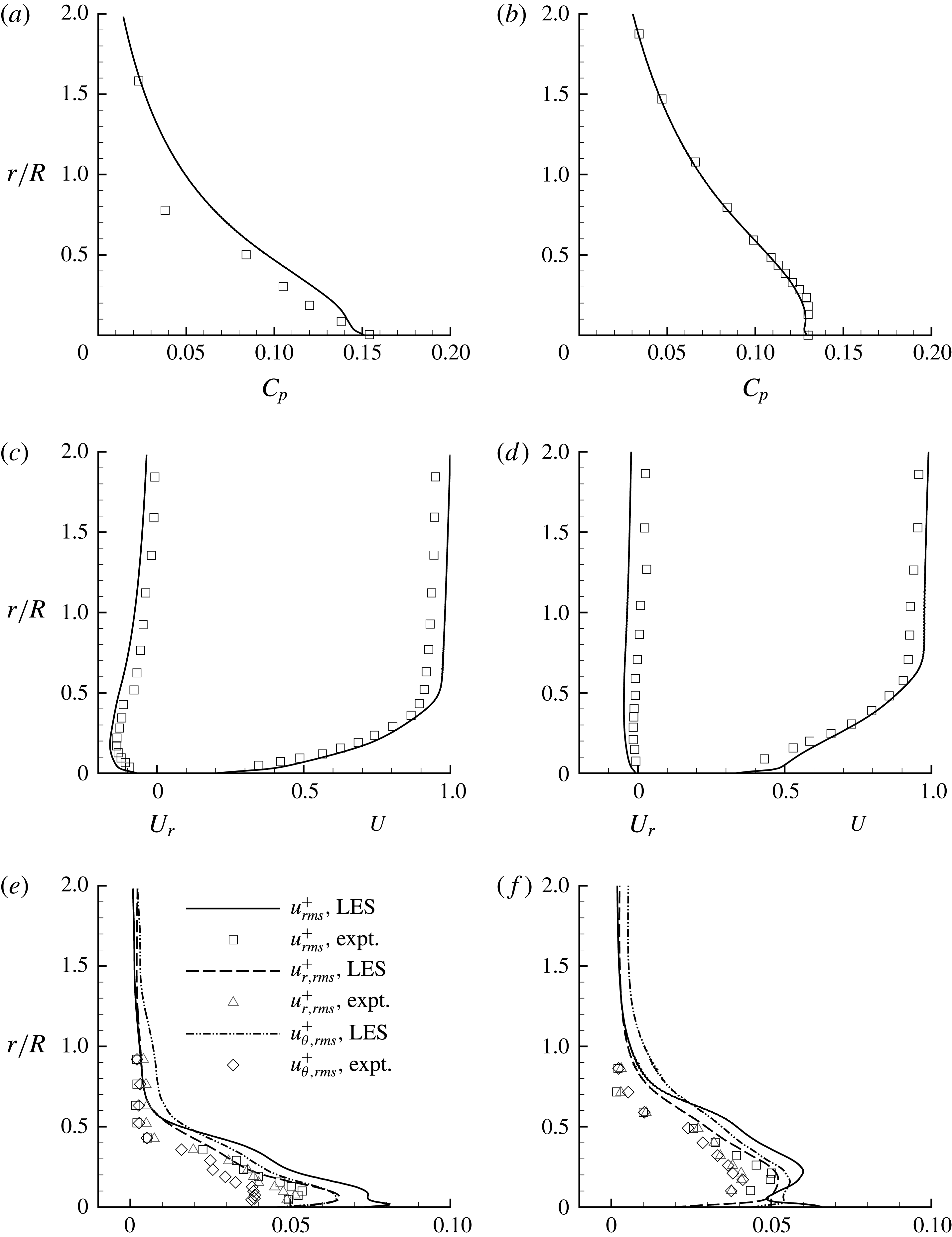
Profiles of pressure coefficient (
 $C_{p}$
) (a,b), mean axial (
 $U$
) and radial (
 $U_{r}$
) velocity (c,d) and r.m.s. of velocity fluctuations (
 $u_{rms}$
,
 $u_{r,rms}$
and
 $u_{\unicode[STIX]{x1D703},rms}$
) (e,f), at
 $x/L=0.904$
(a,c,e) and 0.978 (b,d,f). Symbols show measurements from the experiments of Huang et al. (Reference Huang, Liu, Grooves, Forlini, Blanton and Gowing1992) at
 $Re=1.2\times 10^{7}$
.

Figure 15 compares profiles of pressure and velocity to the experiments of Huang et al. (Reference Huang, Liu, Grooves, Forlini, Blanton and Gowing1992). The radial variation of
 $C_{p}$
as well as the mean axial (
 $U$
) and radial (
 $U_{r}$
) velocities, r.m.s. of velocity fluctuations and Reynolds stress are shown at two streamwise locations on the stern:
 $x/L=0.904$
and
 $0.978$
. The
 $C_{p}$
values obtained from LES show good agreement with those of the experiments. The mean velocities (
 $U$
,
 $U_{r}$
) on the other hand show small differences as compared to the experiments, which can be attributed to the difference in
 $Re$
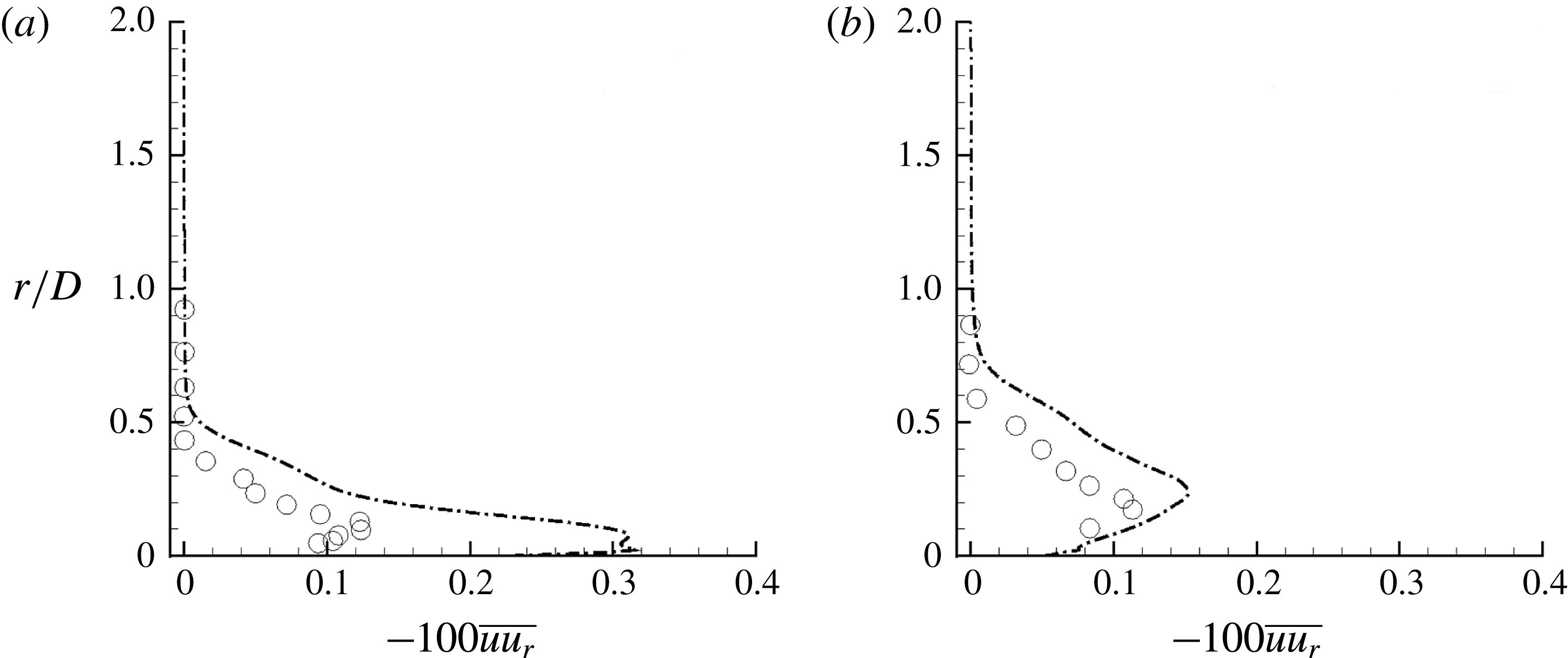
between the simulations and the experiments. The thickening of the hull boundary layer leading to flow separation due to a geometrically induced adverse pressure gradient is evident as we move downstream on the stern. At the same locations, profiles of
 $\overline{uu_{r}}$
are compared to the experiments in figure 16. The simulated values at
 $Re=1.1\times 10^{6}$
are closer to the experiments (
 $Re=1.2\times 10^{7}$
) at the streamwise location
 $x/L=0.978$
as compared to
 $x/L=0.904$
. All of these trends (figures 15 and 16) suggest that the flow field in the stern region is largely insensitive to
 $Re$
at
 $x/L=0.978$
, possibly because of flow separation.
The axisymmetric wake: Reynolds stress (
 $\overline{uu_{r}}$
) at
 $x/L=0.904$
(a) and 0.978 (b). Symbols show measurements from the experiments of Huang et al. (Reference Huang, Liu, Grooves, Forlini, Blanton and Gowing1992) at
 $Re=1.2\times 10^{7}$
.

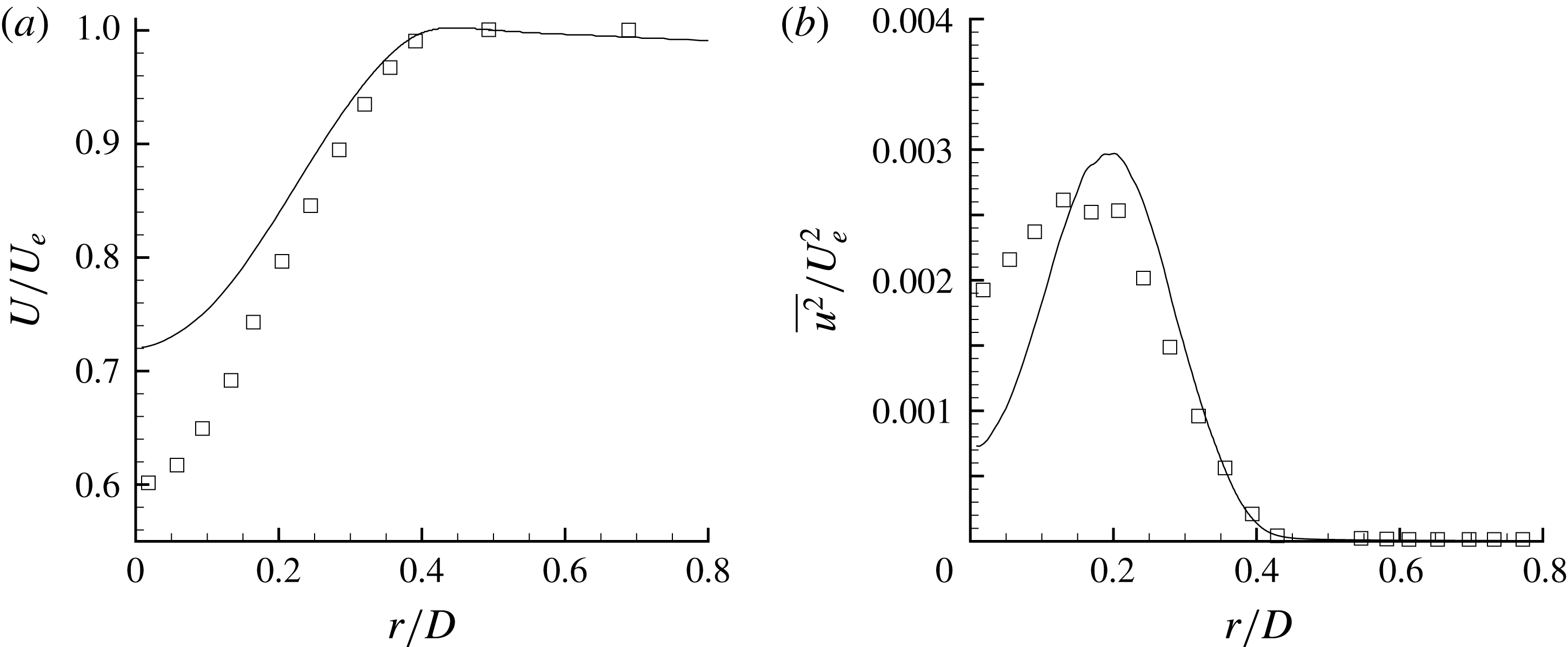
The axisymmetric wake: mean and axial turbulent intensity normalized with edge velocity (
 $U_{e}$
) are compared to Jiménez et al. (Reference Jiménez, Hultmark and Smits2010b
) (symbols) at
 $3D$
downstream of the hull.

The profiles of mean (
 $U$
) and axial turbulence intensity (
 $\overline{u^{2}}$
) at
 $3D$
downstream of the stern are compared to the experiments of Jiménez et al. (Reference Jiménez, Hultmark and Smits2010b
) in figure 17. The wake width matches well with the experiment, whereas the centreline values are underpredicted for both velocity deficit and
 $\overline{u^{2}}$
. The centreline
 $U$
is higher (lower centreline velocity deficit,
 $U_{\infty }-U$
) and the centreline
 $\overline{u^{2}}$
is smaller than that of the experiments. The location of the peak of
 $\overline{u^{2}}$
however, agrees with the experiments. Recall that grid convergence of the drag force and
 $C_{f}$
was discussed and confirmed in § 2.3.
Possible reasons for the mismatch are the confinement and blockage effects in the experiment as discussed earlier. The junction flows due to the semi-infinite sail distorts the axisymmetry and the confinement increases the edge velocity of the wake. Recently, Posa & Balaras (Reference Posa and Balaras2016) simulated fully appended SUBOFF at flow conditions identical to those of Jiménez et al. (Reference Jiménez, Reynolds and Smits2010c
), who reported another set of experiments conducted in the same tunnel and set-up. Posa & Balaras (Reference Posa and Balaras2016) also observed similar differences between their LES results and those from the experiments. Note that the present simulations attempt to match the physical conditions (
 $Re$
and the tripping location) of Jiménez et al. (Reference Jiménez, Hultmark and Smits2010b
), unlike Posa & Balaras (Reference Posa and Balaras2016). Another reason for the mismatch can be the difference in hull boundary layer between the experiments and the simulations. The hull boundary layer in the present work is purely axisymmetric unlike the experiments, where the semi-infinite sail is present. In the absence of the characteristics of hull boundary layer or
 $C_{f}$
on the hull from the experiments, it is impossible to determine whether the present hull boundary layer is identical to that in the experiments. The presence of confinement, junction flows due to the support and the blockage due to instrumentation in the experiments (see Jiménez et al. (Reference Jiménez, Hultmark and Smits2010b
) for details) can also affect the evolution and subsequent separation of the hull boundary layer to form a wake.
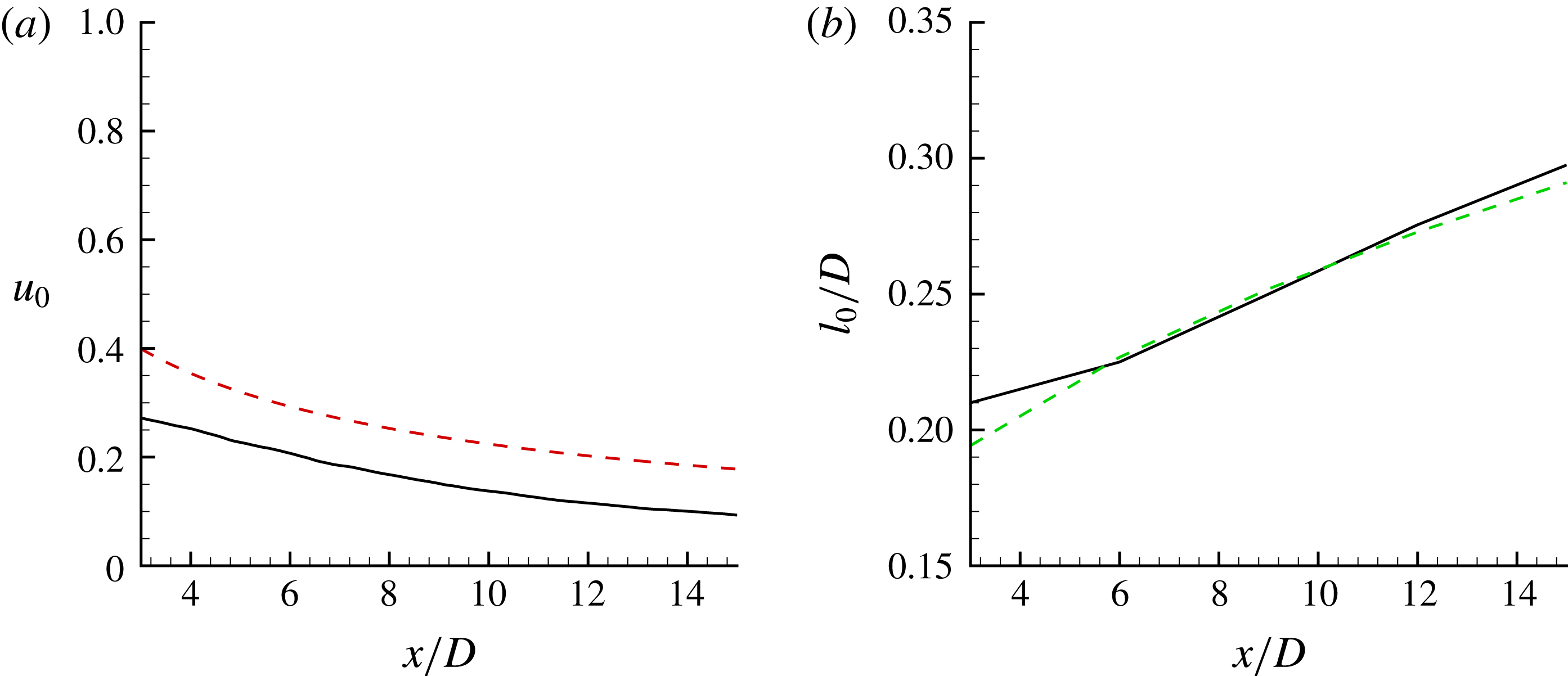
The axisymmetric wake: centreline deficit (
 $u_{0}$
) and half-wake width (
 $l_{0}$
);
 $x$
is the distance measured from the stern. Correlations from Jiménez et al. (Reference Jiménez, Hultmark and Smits2010b
) (dashed lines) are shown for comparison.

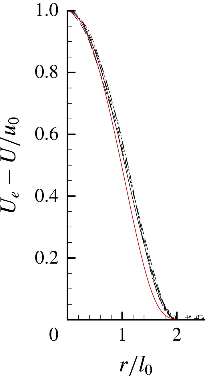
The axisymmetric wake: self-similar mean axial velocity profiles at 3, 6, 9, 12 and 15 diameters downstream of the stern are compared to the correlation of Jiménez et al. (Reference Jiménez, Hultmark and Smits2010b
) (solid red line);
 $U_{e}$
is the velocity at the edge of the wake.

Turbulent wakes are characterized by a centreline deficit (
 $u_{0}$
) and half-wake width (
 $l_{0}$
):
 $$\begin{eqnarray}\displaystyle u_{0}=\frac{U_{e}-U_{r=0}}{U_{e}}, & & \displaystyle\end{eqnarray}$$
where
 $U_{e}$
is the mean axial velocity at the edge of the wake and
 $l_{0}$
is defined as the radial distance from the centreline where the deficit is
 $u_{0}/2$
. The evolution of
 $u_{0}$
and
 $l_{0}$
are compared to the correlations reported by Jiménez et al. (Reference Jiménez, Hultmark and Smits2010b
) in figure 18. The centreline deficit from LES is smaller than that of the experiment, whereas the wake width shows good agreement. The wake is also shown in similarity coordinates and compared to the correlation given by Jiménez et al. (Reference Jiménez, Hultmark and Smits2010b
) in figure 19, showing good agreement.
3.3 The mean flow field
The time-averaged flow field is further averaged in the azimuthal direction to obtain the mean flow field in the
 $xr$
plane. Figure 20 shows mean axial (
 $U$
) and radial (
 $U_{r}$
) velocities in the bow region. The bow region has a strong favourable pressure gradient which is geometrically induced. The boundary layer is tripped at
 $x/D=0.75$
similar to the reference experiment, as mentioned earlier. The thickening of the hull boundary layer can be observed. The value of
 $U_{r}$
is negligible away from the bow region due to high curvature in both the longitudinal and transverse directions. The values of
 $\overline{uu_{r}}$
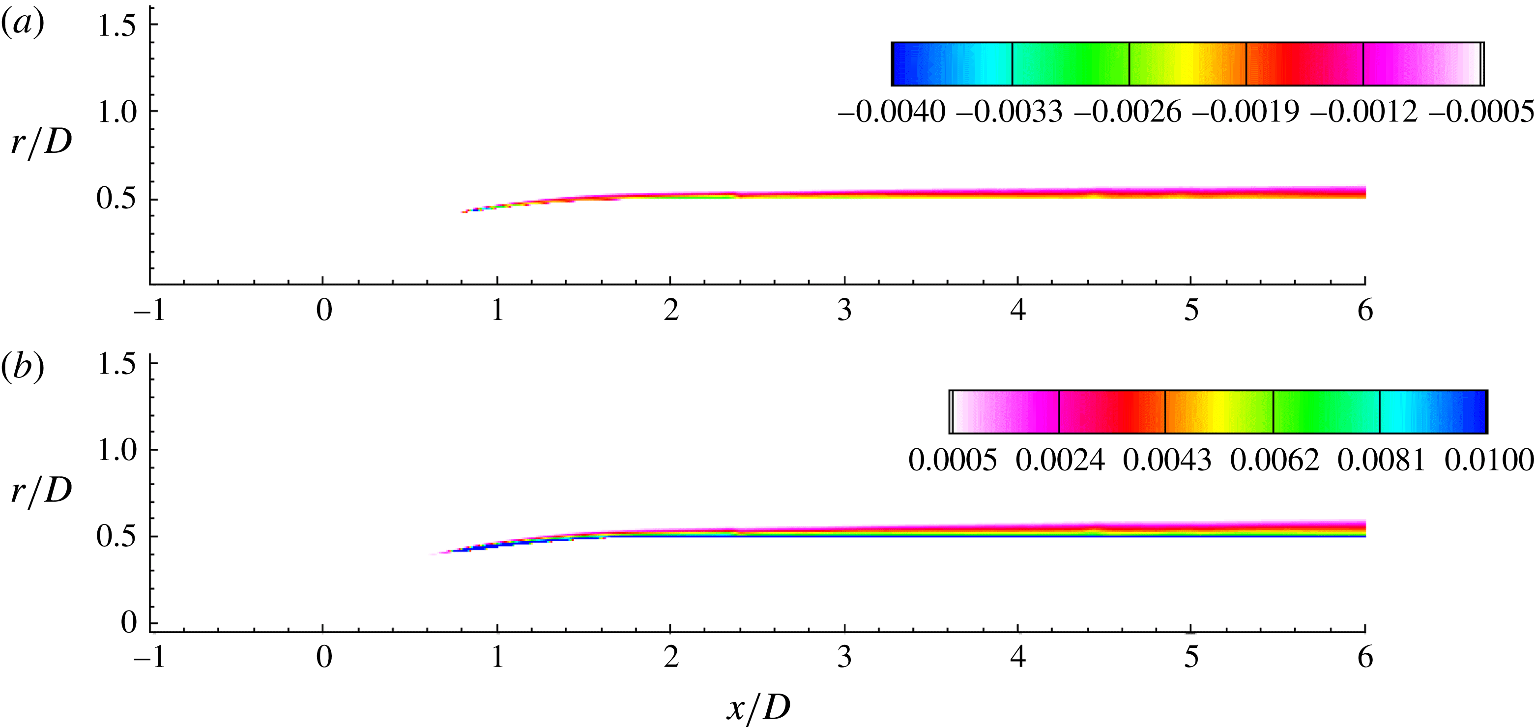
and TKE in the bow region are shown in figure 21. Due to the no-slip boundary condition, there is always a mean shear near the wall. But in order to have production of turbulence,
 $\overline{uu_{r}}<0$
is required in addition to mean shear. Tripping seems to generate this, as shown in figure 21(a). The boundary layer quickly turns turbulent, as evident from the contours of TKE (figure 21
b).
The mean flow field in the bow region: axial velocity (a) and radial velocity (b) in the
 $xr$
plane. The boundary layer is tripped at
 $x/D=0.75$
.

The mean flow field in the bow region: Reynolds stress (a) and TKE (b) in the
 $xr$
plane.

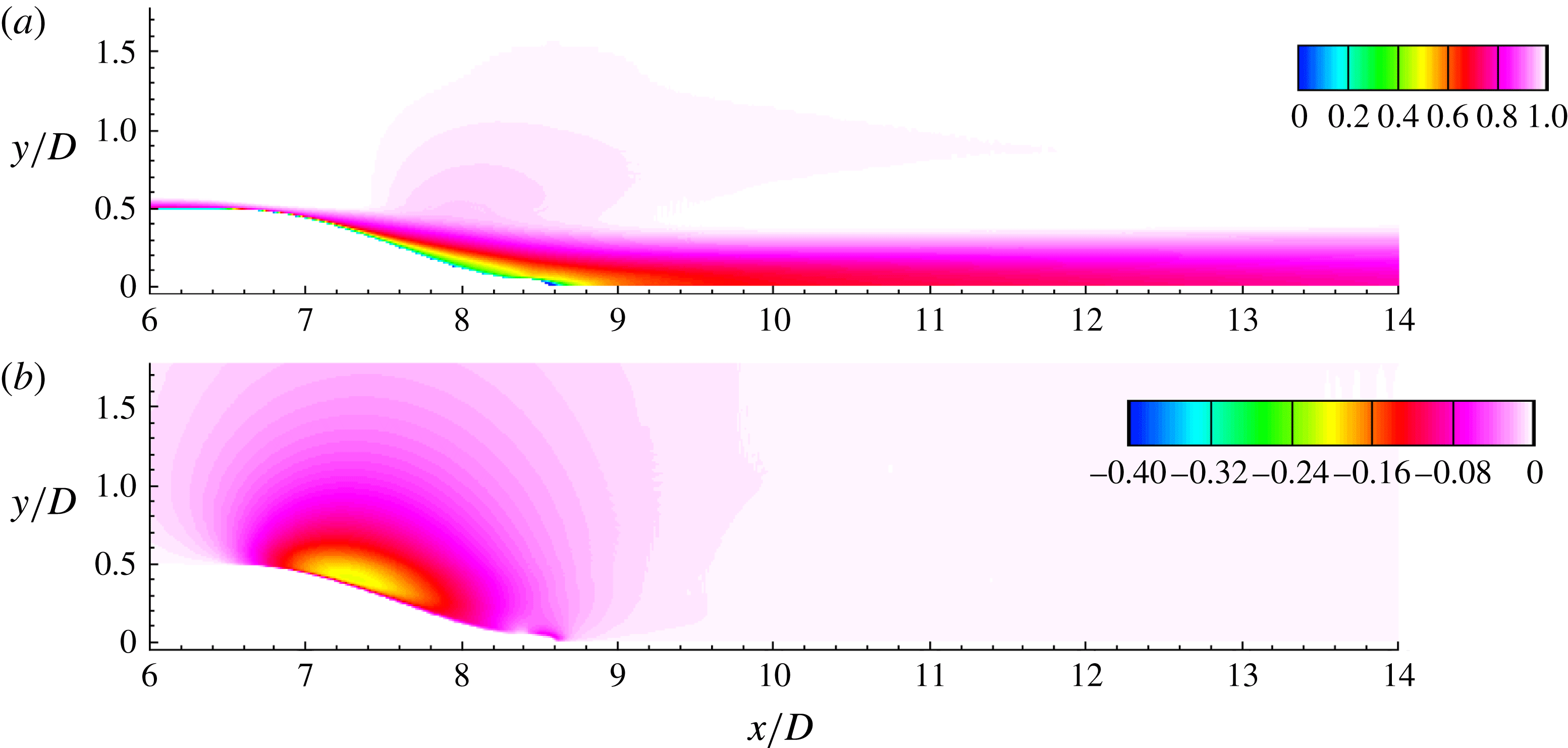
The mean flow field in the stern region: axial velocity (a) and radial velocity (b) in the
 $xr$
plane.

Figure 22 shows
 $U$
and
 $U_{r}$
in the stern region of the hull. The flow separates on the stern due to the adverse pressure gradient. High longitudinal and transverse curvatures lead to high
 $U_{r}$
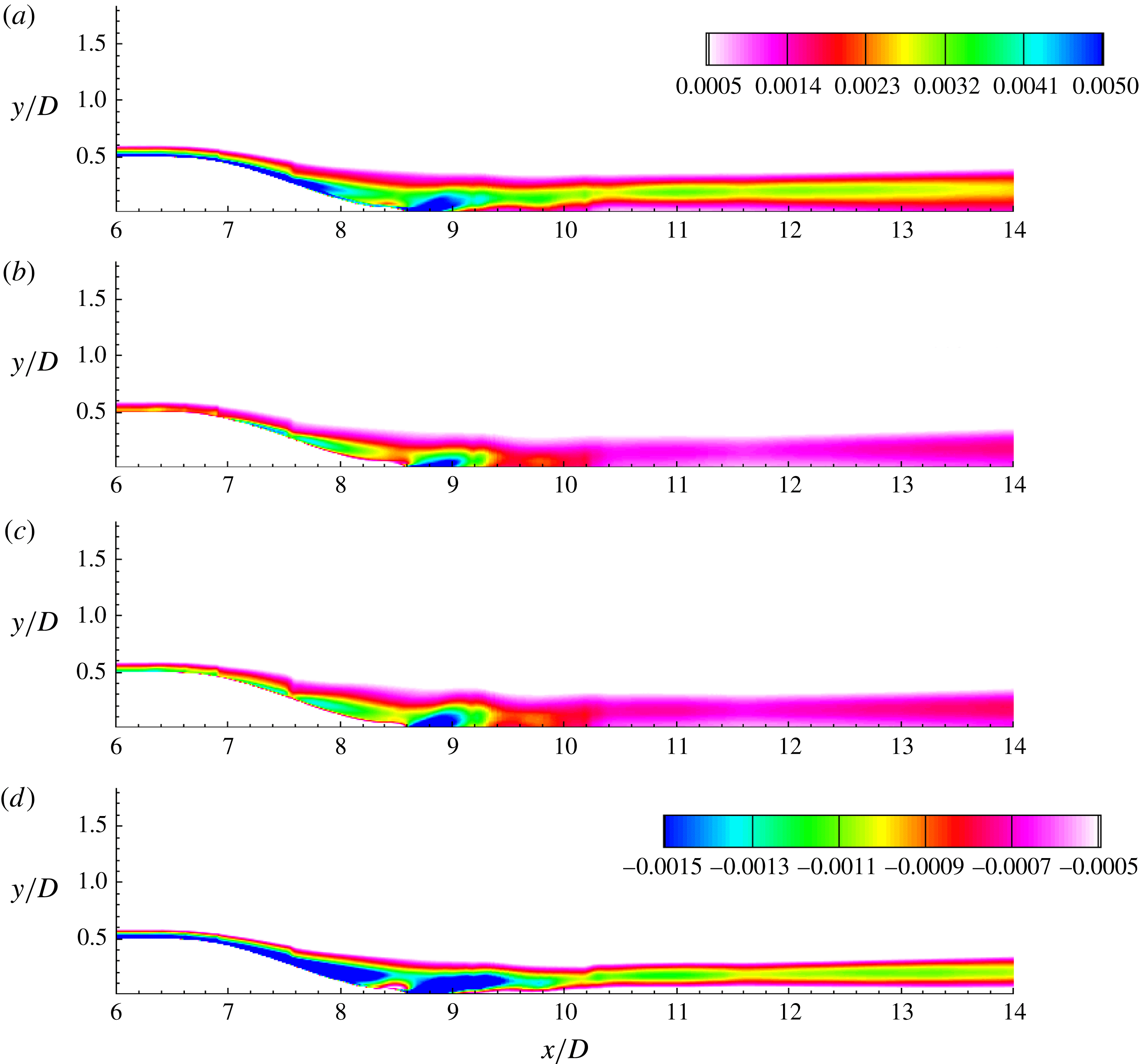
in this region, similar to the bow. Turbulent intensities and
 $\overline{uu_{r}}$
in the stern region are shown in figure 23. The near wake of the hull is dominated by the axial turbulent intensity. All the contours show a local minimum and a local maximum on the centreline and slightly away from the axis, respectively, at any given streamwise location in the wake. This behaviour of turbulent quantities is referred to as the bimodal nature of turbulent wake because the shape of the profiles appears to have two symmetric peaks away from the centreline in the
 $xy$
plane. This is consistent with the past work on SUBOFF (Jiménez et al.
Reference Jiménez, Hultmark and Smits2010b
,Reference Jiménez, Reynolds and Smits
c
; Posa & Balaras Reference Posa and Balaras2016). The origin of this shape lies in the formation of the wake itself. The thin hull boundary layer in the zero-pressure-gradient region of the hull thickens rapidly in the stern region due to the adverse pressure gradient. An adverse pressure gradient is known to suppress turbulence near the wall, as observed by Patel, Nakayama & Damian (Reference Patel, Nakayama and Damian1974) in their experiments on a turbulent boundary layer over an axisymmetric body of revolution. The thickened hull boundary layer with suppressed near-wall turbulence separates to form a wake, which shows peaks at radial offsets from the axis.
The second-order velocity statistics in the stern region: axial (a), radial (b) and azimuthal (c) turbulent intensities and Reynolds stress (d) in the
 $xr$
plane.

3.4 The evolution of an axisymmetric wake
For a self-similar axisymmetric wake, the conservation of axial momentum yields,
 $$\begin{eqnarray}\left.\begin{array}{@{}c@{}}\displaystyle \frac{\text{d}}{\text{d}x}\int _{0}^{\infty }U(U_{\infty }-U)r\,\text{d}r=0\\ \displaystyle \;\Longrightarrow \;\int _{0}^{\infty }U(U_{\infty }-U)r\,\text{d}r=\text{const.}=U_{\infty }^{2}\unicode[STIX]{x1D703}^{2},\end{array}\right\}\end{eqnarray}$$
where,
 $\unicode[STIX]{x1D703}$
is the momentum thickness defined such that,
 $$\begin{eqnarray}\displaystyle \unicode[STIX]{x1D703}^{2}=\frac{1}{U_{\infty }^{2}}\int _{0}^{\infty }U(U_{\infty }-U)r\,\text{d}r. & & \displaystyle\end{eqnarray}$$
As the wake evolves,
 $\unicode[STIX]{x1D703}$
is conserved but the centreline deficit decays and the wake width increases. An important parameter for self-similar axisymmetric wakes is the local Reynolds number which can be defined using
 $u_{0}$
as the velocity scale and an appropriate local length scale. It is convenient to choose
 $\unicode[STIX]{x1D6FF}_{\ast }$
as the local length scale, which is defined such that,
 $$\begin{eqnarray}\displaystyle \unicode[STIX]{x1D6FF}_{\ast }^{2}=\frac{1}{u_{0}}\int _{0}^{\infty }(U_{\infty }-U)r\,\text{d}r. & & \displaystyle\end{eqnarray}$$
Note that
 $l_{0}$
and
 $\unicode[STIX]{x1D6FF}_{\ast }$
are related as,
 $$\begin{eqnarray}\displaystyle l_{0}=\sqrt{2\ln 2}\unicode[STIX]{x1D6FF}_{\ast }. & & \displaystyle\end{eqnarray}$$
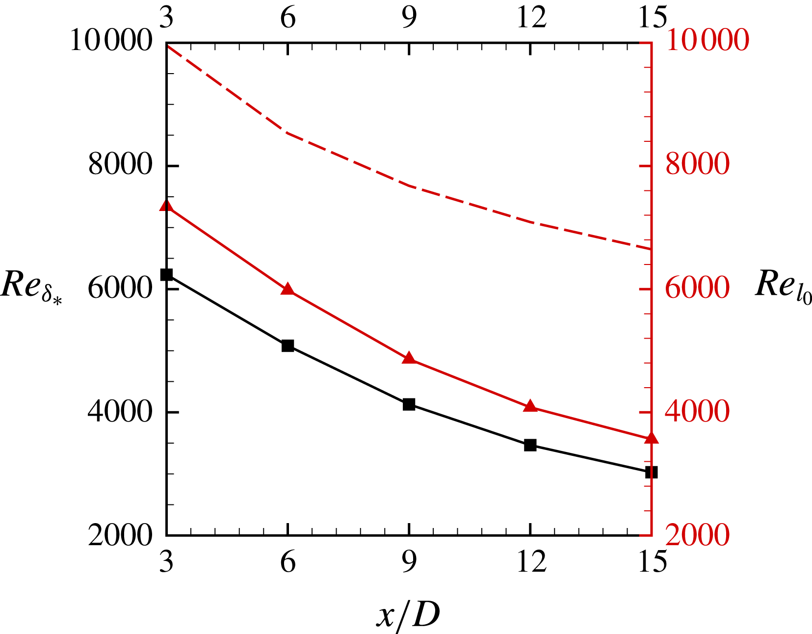
Figure 24 shows the axial evolution of local Reynolds number using
 $\unicode[STIX]{x1D6FF}_{\ast }$
as well as
 $l_{0}$
.
 $Re_{l_{0}}$
is evaluated using the correlations of Jiménez et al. (Reference Jiménez, Hultmark and Smits2010b
) for
 $u_{0}$
and
 $l_{0}$
. As expected, the local Reynolds number shows streamwise decay but the LES result is lower than that from the experiments. A possible reason for this is the presence of the semi-infinite sail in the experiments, which can create an additional velocity defect.
Equation (3.6) along with (3.4) yield,
 $$\begin{eqnarray}\left.\begin{array}{@{}c@{}}\displaystyle u_{0}\unicode[STIX]{x1D6FF}_{\ast }^{2}=U_{\infty }\unicode[STIX]{x1D703}^{2}\\ \displaystyle \;\Longrightarrow \;\frac{\unicode[STIX]{x1D6FF}_{\ast }}{\unicode[STIX]{x1D703}}=\sqrt{\frac{U_{\infty }}{u_{0}}}.\end{array}\right\}\end{eqnarray}$$
Johansson, George & Gourlay (Reference Johansson, George and Gourlay2003) proposed and validated two different self-similar solutions for axisymmetric wakes, namely the high-
 $Re$
(
 $\unicode[STIX]{x1D6FF}_{\ast }\sim x^{1/3}$
) and low-
 $Re$
(
 $\unicode[STIX]{x1D6FF}_{\ast }\sim x^{1/2}$
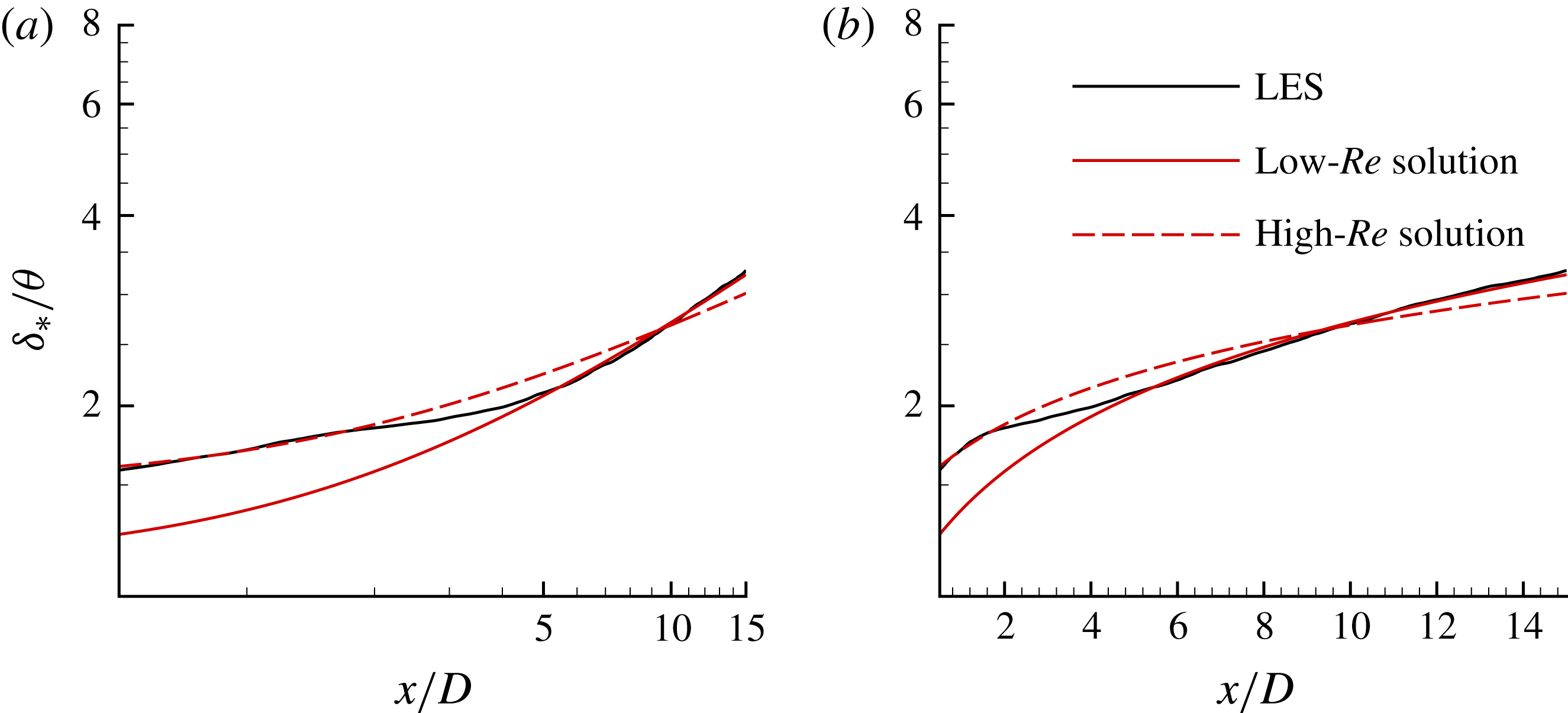
) solutions. Figure 25 shows the streamwise evolution of
 $\unicode[STIX]{x1D6FF}_{\ast }/\unicode[STIX]{x1D703}$
, which is related to
 $u_{0}$
from (3.8). The present result is compared to the two self-similar solutions. The curves,
 $$\begin{eqnarray}\frac{\unicode[STIX]{x1D6FF}_{\ast }}{\unicode[STIX]{x1D703}}=\left\{\begin{array}{@{}ll@{}}\displaystyle 1.17\left(\frac{x+x_{0}}{D}\right)^{1/3};\quad & x/D\leqslant 2\\ \displaystyle 0.78\left(\frac{x+x_{0}}{D}\right)^{1/2};\quad & x/D\geqslant 5\end{array}\right.\end{eqnarray}$$
show a good fit for the present simulated result. Interestingly, the present solution transitions from high-
 $Re$
to low-
 $Re$
similarity solutions between
 $2<x/D<5$
. To the best of our knowledge, this is the first study showing both high-
 $Re$
and low-
 $Re$
similarity solutions for a streamlined body. Note that the virtual origin,
 $x_{0}/D=2.08$
is same as that of Jiménez et al. (Reference Jiménez, Hultmark and Smits2010b
). This difference in the wake behaviour between the present work and the experiments can be attributed to the higher local Reynolds number in the presence of semi-infinite sail.
Evolution of local Reynolds number in the wake. Both
 $Re_{\unicode[STIX]{x1D6FF}_{\ast }}=(u_{0}\unicode[STIX]{x1D6FF}_{\ast })/\unicode[STIX]{x1D708}$
(line with square symbols) and
 $Re_{l_{0}}=(u_{0}l_{0})/\unicode[STIX]{x1D708}$
(line with triangle symbols) are shown and compared to
 $Re_{l_{0}}$
evaluated using the correlations of Jiménez et al. (Reference Jiménez, Hultmark and Smits2010b
) for
 $u_{0}$
and
 $l_{0}$
(dashed line).

It is interesting to note that past studies on a variety of bluff bodies have reported various location for transition from high-
 $Re$
to low-
 $Re$
self-similarity solution for turbulent axisymmetric wakes depending on the wake generators (see Johansson & George (Reference Johansson and George2006) and the references therein). For the present streamlined wake generator, this transition seems to be complete at
 $x/D=5$
, which corresponds to
 $Re_{\unicode[STIX]{x1D6FF}_{\ast }}\approx 5465$
(figure 24).
Axial evolution of
 $\unicode[STIX]{x1D6FF}_{\ast }/\unicode[STIX]{x1D703}$
compared to the similarity laws proposed for axisymmetric wakes in log–log (a) and log–linear (b) axes. Both low-
 $Re$
(
 ${\sim}x^{1/2}$
) and high-
 $Re$
(
 ${\sim}x^{1/3}$
) similarity solutions are shown.

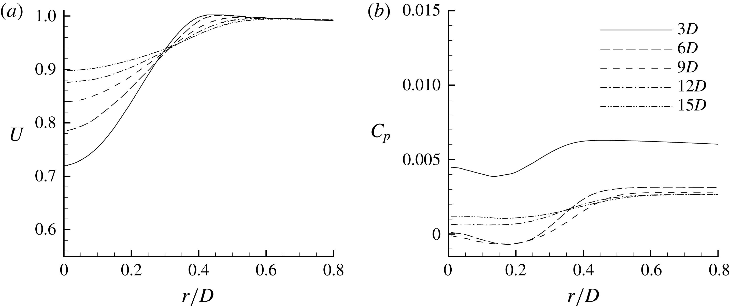
Profiles of
 $U$
and
 $C_{p}$
are extracted at various streamwise locations from
 $3D$
to
 $15D$
downstream of the hull, as shown in figure 26. Slow expansion of the axisymmetric wake and the diffusion of the shear layer at the edge of the wake are evident in the profiles of
 $U$
as we go downstream in the wake.
 $C_{p}$
is small at all locations, however there is a small radial gradient, which decreases moving downstream.
The axisymmetric wake: (a)
 $U$
and (b)
 $C_{p}$
at 3, 6, 9, 12 and 15 diameters downstream of the stern.

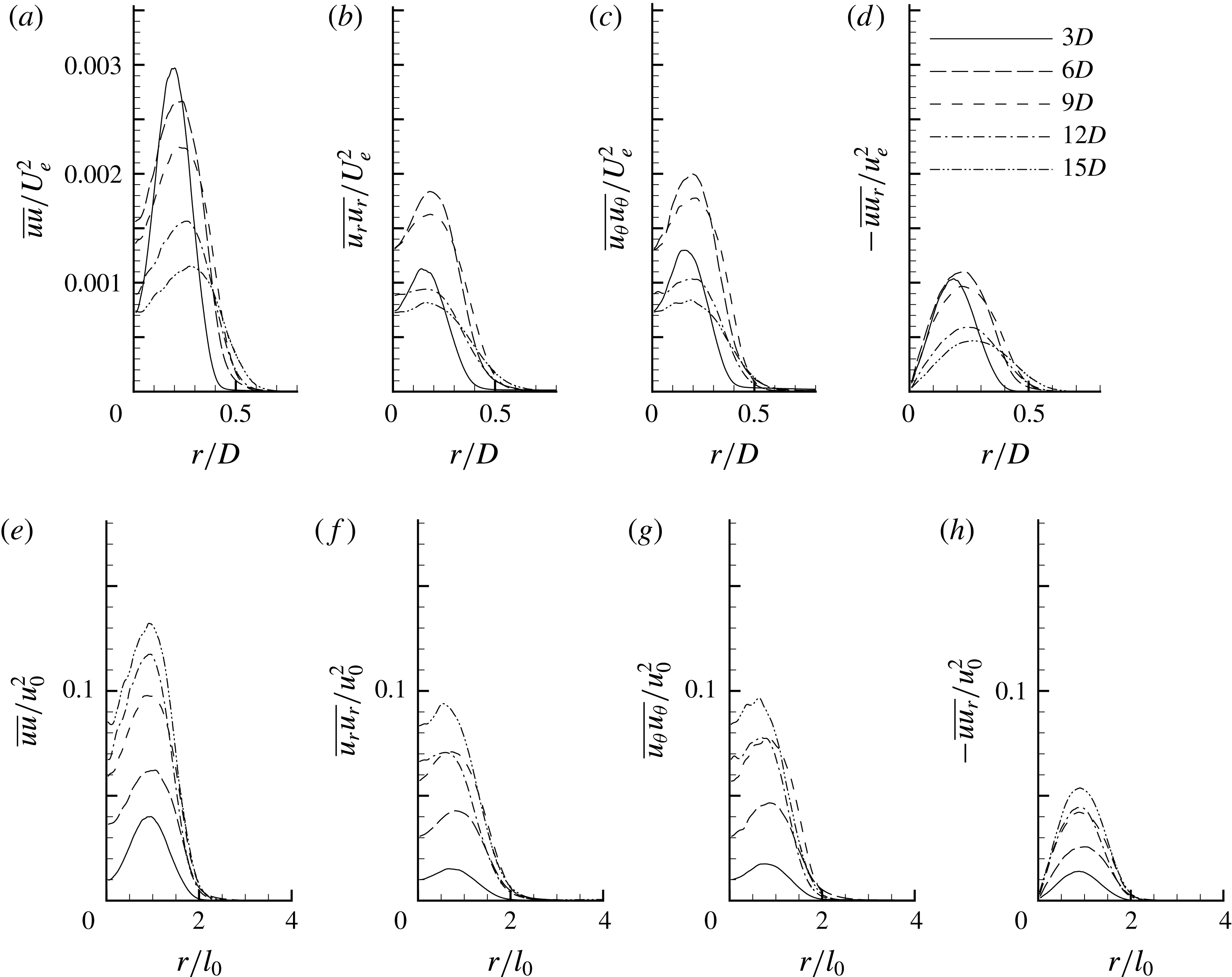
Profiles of turbulent intensities and Reynolds stress are shown in figure 27 in both physical (a–d) and similarity (e–h) coordinates at the same streamwise locations as those of figure 26. The peak of the axial turbulent intensity decreases monotonically going downstream whereas, there is a slight increase in the radial and azimuthal turbulent intensities from
 $3D$
to
 $6D$
, followed by a decrease until the last location. The peaks of all of the profiles drift radially outward due to slow radial spreading of the turbulent wake. The same quantities in similarity coordinates do not show any such drift i.e. the peaks at all of the locations in the wake are located at
 $r/l_{0}=1$
, identical to the observations of Jiménez et al. (Reference Jiménez, Hultmark and Smits2010b
). Note that the peak values of all the quantities increase monotonically moving downstream in the wake despite a streamwise decrease in their magnitudes (figure 27
e–h) because of the rapid streamwise decay of the centreline deficit (
 $u_{0}$
). In other words,
 $u_{0}^{2}$
decreases more rapidly as compared to turbulent intensities and Reynolds stress as we move downstream in the wake. Consistent with the previous studies reported in the literature for this geometry, there is no sign of self-similarity in the second-order velocity statistics over the length of the simulated domain.
The axisymmetric wake: (a,e)
 $\overline{uu}$
, (b,f)
 $\overline{u_{r}u_{r}}$
, (c,g)
 $\overline{u_{\unicode[STIX]{x1D703}}u_{\unicode[STIX]{x1D703}}}$
and (d,h)
 $\overline{uu_{r}}$
at 3, 6, 9, 12 and 15 diameters downstream of the stern in physical (a–d) and similarity coordinates (e–h).
 $U_{e}$
and
 $u_{0}$
are edge velocity and centreline deficit respectively.

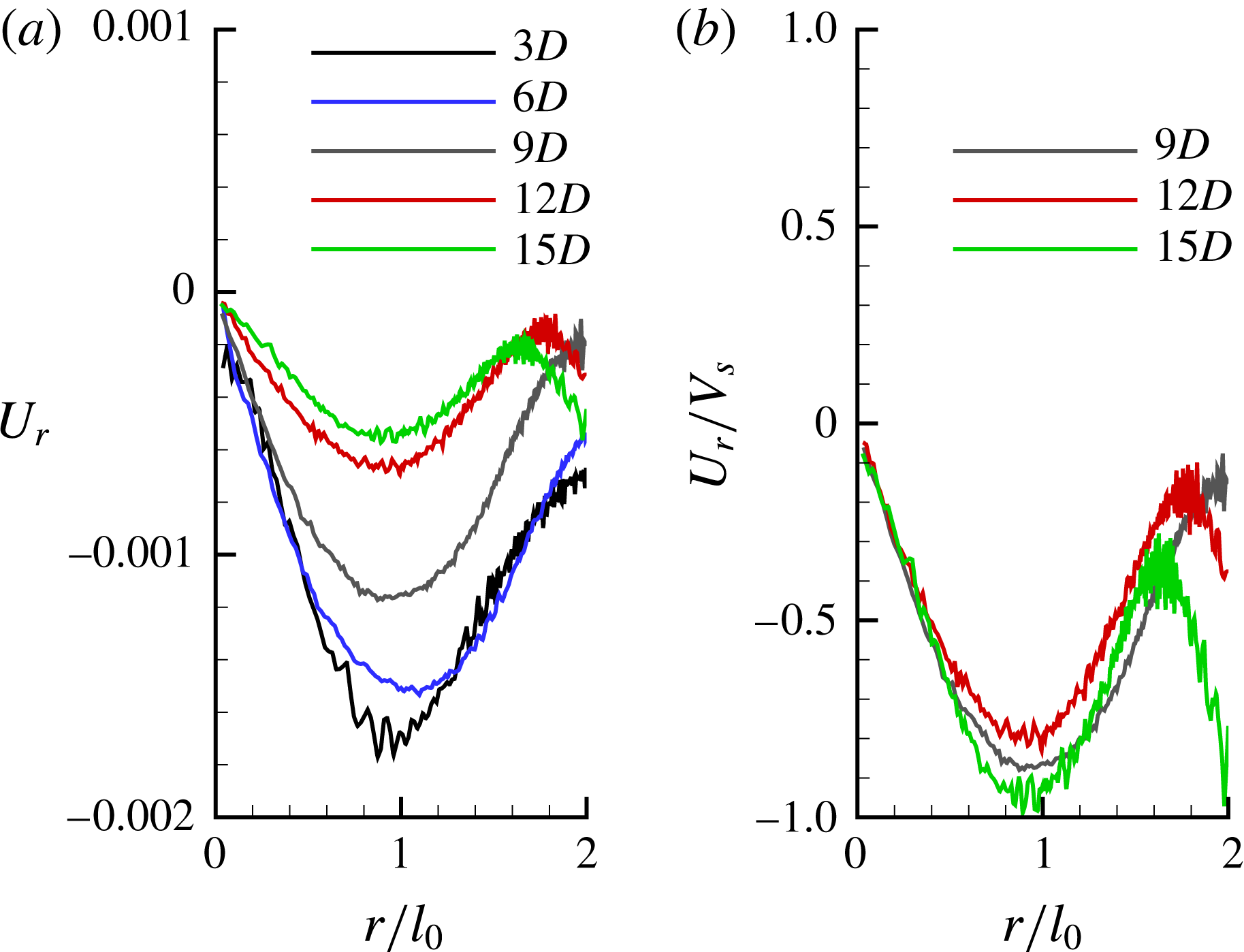
Mean radial velocities are often neglected in the studies of free shear flows, but they are important quantities when near field and entrainment effects are important. The transient length needed to achieve self-similarity also depends on entrainment for shear flows, as demonstrated by Babu & Mahesh (Reference Babu and Mahesh2004) for both laminar and turbulent round jets. Profiles of mean radial velocity (
 $U_{r}$
) are shown in figure 28(a). The value of
 $U_{r}$
is small and negative at all of the locations shown and the peaks occur at
 $r/l_{0}=1$
. Note that the profiles are not symmetric about
 $r/l_{0}=1$
and
 $U_{r}$
does not go to zero at the edge of the wake. In fact, it is negative and higher in magnitude closer to the hull due to entrainment caused by the separation of the hull boundary layer on the stern. This phenomenon of entrainment by separated shear layers has been studied in the past (see Stella, Mazellier & Kourta (Reference Stella, Mazellier and Kourta2017) and references therein). It can be shown that
 $V_{s}=u_{0}(\text{d}l_{0}/\text{d}x)$
is an appropriate scale for
 $U_{r}$
. Scaling the profiles of
 $U_{r}$
with
 $V_{s}$
shows a reasonable collapse beyond
 $9D$
, as shown in figure 28(b).
The axisymmetric wake:
 $U_{r}$
at 3, 6, 9, 12 and 15 diameters (a) and
 $U_{r}$
scaled with
 $V_{s}$
beyond 9 diameters (b) downstream of the stern;
 $V_{s}=u_{0}(\text{d}l_{0}/\text{d}x)$
is the mean radial velocity scale.

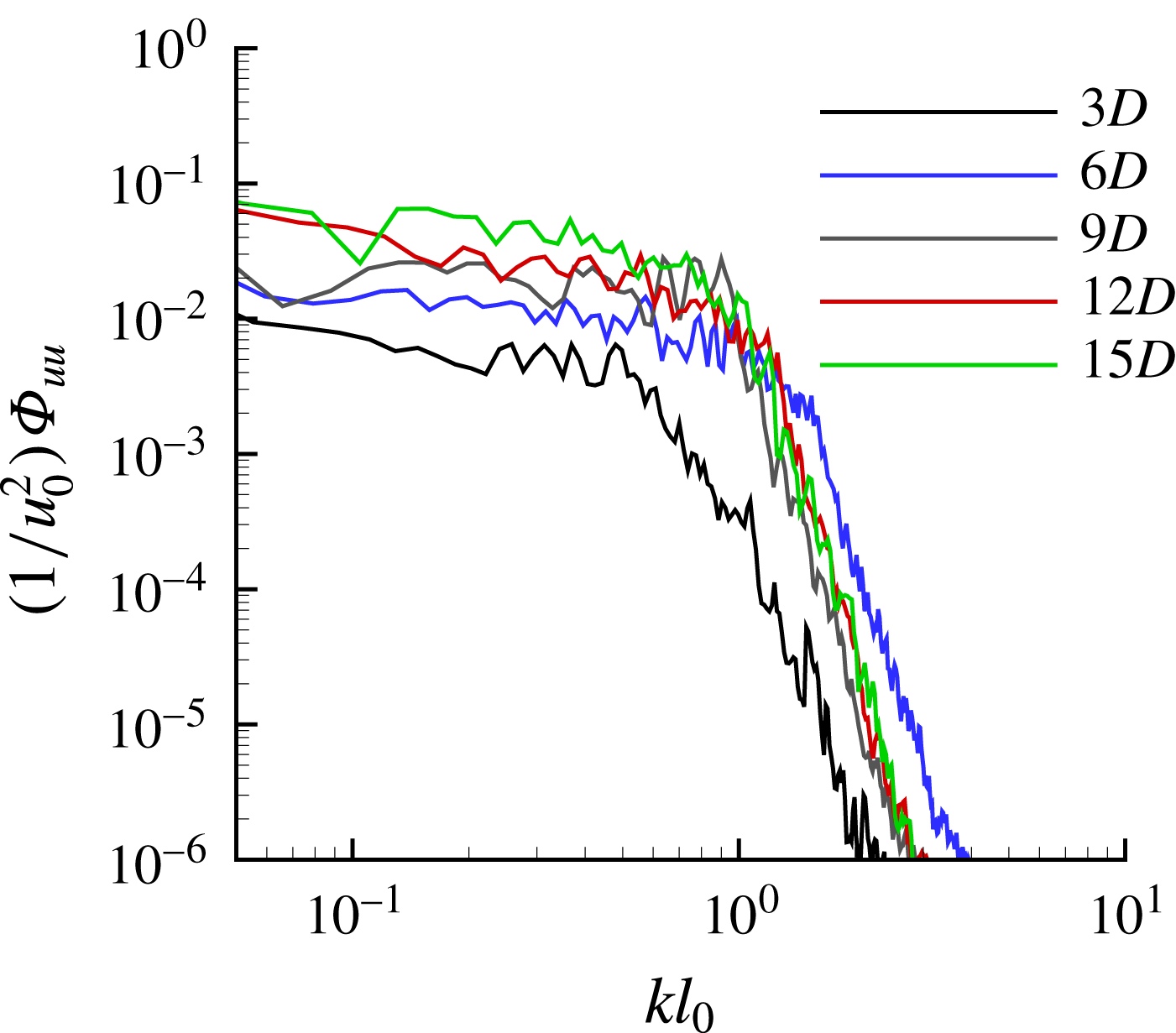
Energy spectra of the streamwise velocity at the centreline are shown in figure 29. Note that, there is no sign of the coherent shedding (see figure 29
b), usually observed for bluff bodies at high
 $Re$
, consistent with the observations of Jiménez et al. (Reference Jiménez, Hultmark and Smits2010b
) at the present
 $Re$
.
Energy spectra of streamwise velocity component at centreline (
 $r/l_{0}=0$
) in the wake at 3, 6, 9, 12 and 15 diameters downstream of the stern.

4 Summary
Wall-resolved LES is used to simulate flow over axisymmetric hull (SUBOFF without appendages) at
 $Re=1.1\times 10^{6}$
at zero angle of pitch and yaw. The length of the computational domain and the level of grid resolution are significantly higher than most past work and chosen to capture the axisymmetric wake up to 15 diameters downstream of the body without any confinement effect. Grid convergence studies have been performed to ensure grid independent numerical solutions. LES results are compared to the experimental data of Huang et al. (Reference Huang, Liu, Grooves, Forlini, Blanton and Gowing1992) for
 $C_{p}$
,
 $C_{f}$
and the mean velocity and pressure profiles on the stern. Values of
 $C_{p}$
and scaled
 $C_{f}$
show good agreement with the experiment and the mean velocity and pressure profiles show similar trends. The axisymmetric wake of the hull is compared to the experiments of Jiménez et al. (Reference Jiménez, Hultmark and Smits2010b
), showing good agreement with the wake width but with a smaller centreline deficit, probably due to blockage and confinement effects in the experimental set-up.
The hull boundary layer and the wake of the hull are discussed in detail. The boundary layer turns turbulent after tripping and evolves until its separation on the stern to form a wake. Comparisons of the axisymmetric TBL with a planar TBL under similar conditions for first- and second-order velocity statistics show that both are similar very close to the surface. However, TKE and Reynolds stress in the axisymmetric TBL decay much more rapidly compared to the planar TBL away from the surface. This appears to be the effect of curvature, which tends to suppress long structures of the log region of the TBL. The axisymmetric wake shows self-similarity in the mean streamwise velocity but not in the turbulence intensities, even up to fifteen diameters downstream of the hull. The peaks of turbulence intensities and Reynolds stress in similarity coordinates are located at a half-wake width away from the axis at all of the streamwise locations. All of these observations are consistent with the past studies. The profiles of mean radial velocity and Reynolds stress show reasonable collapse, mainly in the far wake when scaled with appropriate scales. The present work shows that as the wake evolves downstream, it shifts from a high-
 $Re$
to low-
 $Re$
equilibrium similarity solution, as theoretically proposed by Johansson et al. (Reference Johansson, George and Gourlay2003) and observed only for wakes of bluff bodies in the past.
Acknowledgements
This work is supported by the United States Office of Naval Research (ONR) under ONR grant N00014-14-1-0289 with Dr K.-H. Kim as technical monitor. The computations were made possible through the computing resources provided by the US Army Engineer Research and Development Center (ERDC) in Vicksburg, Mississippi on the Cray XE6, Copper and Garnet of High Performance Computing Modernization program (HPCMP). This research partly used the computer time provided by the Innovative and Novel Computational Impact on Theory and Experiment (INCITE) program on the resources of the Argonne Leadership Computing Facility (ALCF), which is a DOE Office of Science User Facility supported under Contract DE-AC02-06CH11357. The authors thank Mr S. Anantharamu for his help with the grid pre-processing needed for the massively parallel computations reported in this paper.