1. Introduction
Thermoacoustic instability occurs when the acoustic field in a confinement is amplified in the presence of an unsteady heat source. The amplification of the acoustic field happens when the heat release rate fluctuations are in phase with the inherent acoustic pressure perturbations (Rayleigh Reference Rayleigh1878). Many power generating systems and propulsion systems such as gas turbine engines and rocket motors are susceptible to thermoacoustic instability (McManus, Poinsot & Candel Reference McManus, Poinsot and Candel1993). Apart from causing structural damage, thermoacoustic oscillations often result in reduced performance and increased heat transfer rates.
A complete understanding of such thermoacoustic oscillations is difficult owing to the complexity of the systems where this instability occurs. This difficulty can be bypassed by employing a canonical system that retains the essential features of thermoacoustic systems, but is simple enough for detailed analysis. A horizontal Rijke tube, a horizontal duct with a concentrated heat source, is such a prototypical system often chosen to study the intricacies of thermoacoustic instabilities in the past (Matveev Reference Matveev2003; Balasubramanian & Sujith Reference Balasubramanian and Sujith2008; Subramanian et al. Reference Subramanian, Mariappan, Sujith and Wahi2010; Juniper Reference Juniper2011; Mariappan Reference Mariappan2011). The heat source in a Rijke tube can be a flame or an electrically heated wire mesh. In a traditional vertical Rijke tube, the mean flow is set up by buoyancy. The vertical configuration avoids the need for an external means to create the mean flow. However, the flow rate will be dependent on the heat release rate and it is not possible to control the flow rate independently. In contrast, in a horizontal Rijke tube, the mean flow has to be established by external means and hence can be controlled independently of the heat release rate. In addition to the mean flow rate, the main system parameters that decide the stability of the system are the heater power, the location of the heat source and the acoustic losses in the duct. Thermoacoustic systems are nonlinear. Such nonlinear systems exhibit a sudden change in their qualitative behaviour for an infinitesimal change in any of the system parameters (Matveev Reference Matveev2003; Balasubramanian & Sujith Reference Balasubramanian and Sujith2008; Subramanian et al. Reference Subramanian, Mariappan, Sujith and Wahi2010; Kabiraj et al. Reference Kabiraj, Saurabh, Wahi and Sujith2012; Kabiraj & Sujith Reference Kabiraj and Sujith2012).
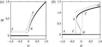
The phenomenon where a nonlinear dynamical system shows a sudden qualitative change in behaviour for an infinitesimal change in system parameters is termed ‘bifurcation’ in dynamical systems theory. If this change takes the system from a stable steady state to an oscillatory state, it is called a ‘Hopf bifurcation’ (Hilborn Reference Hilborn2000; Strogatz Reference Strogatz2000). Hopf bifurcation can be of two types, supercritical and subcritical. In a supercritical Hopf bifurcation, the system remains in the non-oscillatory state until the control parameter reaches the critical value. Once the value of the control parameter crosses the critical value, the non-oscillatory state becomes unstable and the system goes to the oscillatory state. This change is marked by the presence of a low-amplitude stable limit cycle. The parameter value at which the system loses its stability, i.e. when the non-oscillatory state becomes unstable, is called the ‘Hopf point’ (point B in figure 1 a,b).
Bifurcation characteristics of a measure
 $M$
when a control parameter
 ${\it\mu}$
is varied: (a) supercritical bifurcation; (b) subcritical bifurcation. In supercritical bifurcation, as the control parameter reaches the value of zero, low-amplitude stable limit cycle oscillations are born. Unlike the supercritical bifurcation, large-amplitude oscillatory solutions are present right at the onset of instability in the case of subcritical bifurcation. The system is bistable in the hysteresis region BCEF and the stability of the system is dependent on the initial conditions in this region: ●, stable oscillatory solutions; ○, unstable oscillatory solutions. The panels are obtained from the normal-form equations of Hopf bifurcation.

In the case of a subcritical bifurcation, the system experiences large-amplitude oscillations right at the onset of instability. Moreover, while changing the operating conditions along the reverse path, the control parameter needs to be varied to a value significantly beyond the critical value to bring the system back to a non-oscillatory state. The parameter value at which the system regains its stability when the control parameter is varied along the reverse path (point
 $E$
in figure 1
b), is called the fold point (Hilborn Reference Hilborn2000; Strogatz Reference Strogatz2000; Subramanian et al.
Reference Subramanian, Mariappan, Sujith and Wahi2010). The existence of a fold point along with the Hopf point results in the presence of a hysteresis region (region BCEF in figure 1
b). The system is said to be bistable in the hysteresis region, as the system can remain in two different asymptotic states depending upon the initial conditions. However, in a supercritical bifurcation, the stability of the system is independent of the initial conditions. As soon as the control parameter value is brought back to the critical value, the system goes back to the non-oscillatory state in the case of a supercritical bifurcation (figure 1
a). Thus the presence of the hysteresis region can be used as a good indicator to establish the presence of subcritical Hopf bifurcation (Hilborn Reference Hilborn2000; Strogatz Reference Strogatz2000).
Experimental and numerical studies on horizontal Rijke tube show that the transition to instability can happen through a subcritical Hopf bifurcation (Balasubramanian & Sujith Reference Balasubramanian and Sujith2008; Subramanian et al. Reference Subramanian, Mariappan, Sujith and Wahi2010; Juniper Reference Juniper2011; Mariappan Reference Mariappan2011; Gopalakrishnan & Sujith Reference Gopalakrishnan and Sujith2014). A model of the horizontal Rijke tube proposed by Balasubramanian & Sujith (Reference Balasubramanian and Sujith2008) captured many of the features, including the subcritical nature of the transition, often observed in experiments. Later, Subramanian et al. (Reference Subramanian, Mariappan, Sujith and Wahi2010) used the method of numerical continuation to extensively investigate the effect of various system parameters on the dynamics of Rijke oscillations in the Rijke tube model of Balasubramanian & Sujith (Reference Balasubramanian and Sujith2008). They showed that, for this model, the transition to instability happens through a subcritical Hopf bifurcation for all system parameters. Mariappan (Reference Mariappan2011) performed experiments in a horizontal Rijke tube by changing the heater power and he also observed subcritical transition to limit cycle oscillations.
A system exhibiting subcritical transition will remain non-oscillating in the bistable region for perturbations within the basin of attraction of the fixed point. On the other hand, the system will oscillate in the bistable region if the amplitude of perturbations is outside the basin boundary of the fixed point, but well within the basin of attraction of the limit cycle. The process in which a system remains stable for perturbations of low amplitude, but becomes unstable for a perturbation of finite amplitude is termed ‘triggering’ in the thermoacoustic literature (Dickinson Reference Dickinson1962; Brownlee Reference Brownlee1964; Cantrell, McClure & Hart Reference Cantrell, McClure and Hart1965; Brownlee & Kimbell Reference Brownlee and Kimbell1966; Marxman & Wooldridge Reference Marxman and Wooldridge1969; Levine & Baum Reference Levine and Baum1982; Wicker et al. Reference Wicker, Greene, Kim and Yang1996).
Juniper (Reference Juniper2011) used the model of Balasubramanian & Sujith (Reference Balasubramanian and Sujith2008) to study the phenomenon of triggering in a thermoacoustic system. He proposed a procedure based on adjoint looping of the nonlinear governing equations to find the lowest initial energy required to trigger the system. He found that the transition to instability is subcritical when the heater power is chosen as a control parameter, and this transition to stable limit cycle oscillations happens via an unstable periodic solution.
Zinn & Lieuwen (Reference Zinn, Lieuwen, Lieuwen and Yang2005) reported that perturbations of the order of background noise levels are sufficient to trigger a thermoacoustic system. Lieuwen & Banaszuk (Reference Lieuwen and Banaszuk2005) expressed the view that the turbulent fluctuations present in practical thermoacoustic systems can be thought of as additive and parametric sources of noise. Waugh, Geuß & Juniper (Reference Waugh, Geuß and Juniper2011) and Waugh & Juniper (Reference Waugh and Juniper2011) performed a detailed numerical study on the effect of various types of noise, such as white, pink and blue noise, on triggering a thermoacoustic system to instability using the model of horizontal Rijke tube proposed by Balasubramanian & Sujith (Reference Balasubramanian and Sujith2008). White noise is one in which energy is equally distributed among all the frequencies and the power spectrum is flat as in the case of white light. In the case of pink noise, the amount of energy content in a particular frequency is inversely proportional to the value of the frequency and the power spectrum varies as
 $1/f$
, where
 $f$
is the frequency. Blue noise will have a power spectrum that varies as
 $f$
and consequently the higher frequencies contain more energy (Ojalvo & Sancho Reference Ojalvo and Sancho1999).
Waugh et al. (Reference Waugh, Geuß and Juniper2011) found that triggering is strongly dependent on the strength and the colour of the noise. They suggested that pink noise is the most effective in triggering the system to instability, whereas blue noise can even inhibit the phenomenon of triggering. Waugh et al. (Reference Waugh, Geuß and Juniper2011) also observed that a thermoacoustic system can become unstable in the presence of noise even if it is in the linearly stable regime. They reported that the system will reach the state of stable limit cycle oscillations from a non-oscillatory state via a state of unstable limit cycle oscillations. Waugh & Juniper (Reference Waugh and Juniper2011) found that the system will dislodge itself from the oscillatory solution if the noise amplitude is high. They introduced stochastic stability maps to visualize practical stability of a thermoacoustic system in the presence of noise.
Jegadeesan & Sujith (Reference Jegadeesan and Sujith2013) showed experimentally that, for a ducted non-premixed flame, noise-induced triggering to instability is possible. They also obtained the deterministic and stochastic stability maps. Using nonlinear time-series analysis, they constructed phase portraits and found that, when the system is triggered, the transition to instability happens via an unstable limit cycle oscillation, as predicted by Juniper (Reference Juniper2011). Jegadeesan & Sujith (Reference Jegadeesan and Sujith2013) experimentally validated the observation made by Waugh et al. (Reference Waugh, Geuß and Juniper2011) that the transition to instability happens even when the noise level is significantly below the triggering amplitude. However, Waugh et al. (Reference Waugh, Geuß and Juniper2011) and Waugh & Juniper (Reference Waugh and Juniper2011) reported no change in the amplitude of the limit cycle oscillations in the presence of noise. In contrast, Jegadeesan & Sujith (Reference Jegadeesan and Sujith2013) reported a reduction in amplitude of the limit cycle oscillations in the presence of noise. They attributed this decrease in amplitude to a decrease in the correlation between the pressure oscillations and the heat release rate fluctuations in the presence of external noise.
The existing literature in thermoacoustics focuses on noise-induced triggering (Juniper Reference Juniper2011; Waugh et al. Reference Waugh, Geuß and Juniper2011; Waugh & Juniper Reference Waugh and Juniper2011; Jegadeesan & Sujith Reference Jegadeesan and Sujith2013). In noise-induced triggering, the focus is on the ability of the noise pulses or continuous noise, both of which can be coloured or white, to trigger a system, which is otherwise linearly stable, to instability. In a triggering study, the value of the control parameter will be maintained constant and the intensity of the noise will be progressively increased. The system will be exposed to noise of a given intensity for a definite amount of time. It is reported that both the intensity of the noise and the duration for which noise is applied have an effect on the triggering (Waugh & Juniper Reference Waugh and Juniper2011; Jegadeesan & Sujith Reference Jegadeesan and Sujith2013).
Outside the context of thermoacoustics, the effect of noise on the transitions that can happen in nonlinear systems is well studied and it is referred to as noise-induced transitions (NITs) (Horsethemke & Lefever Reference Horsethemke and Lefever2006). NIT refers to the effect of fluctuations on the dynamics of a system and the appearance of novel dynamical features that are not present in the deterministic system. It is found that noise can induce new dynamical states and bifurcations (Horsethemke & Lefever Reference Horsethemke and Lefever2006; Aumaitre, Mallick & Petrelis Reference Aumaitre, Mallick and Petrelis2007). In this work we study such NITs that can happen in a prototypical thermoacoustic system.
Our study on NIT differs from the studies on noise-induced triggering in the methodology employed. We keep the intensity of noise constant and we increase the control parameter such that the system reaches the oscillatory state from a non-oscillatory state. In a similar fashion, we decrease the control parameter to bring the system back to a non-oscillatory state from an oscillatory state for the same intensity of noise. In our study, the time during which the system is exposed to a specific intensity of noise is at least 1800 s. This exposure time is long enough to be considered infinite compared to the 90 s that was used in an experimental study (Jegadeesan & Sujith Reference Jegadeesan and Sujith2013) and 18 s that was used in a numerical study (Waugh & Juniper Reference Waugh and Juniper2011) on noise-induced triggering.
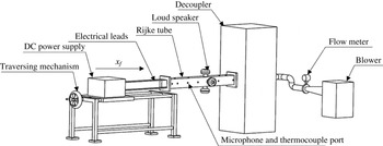
Schematic of the experimental set-up. A blower is used to provide the mean flow and a flow meter is used to measure the flow rate. A DC power supply unit is used to heat the wire mesh.

We experimentally investigate the effect of noise on the hysteresis characteristics of a prototypical thermoacoustic system, a horizontal Rijke tube. In particular, we examine how the width of the bistable zone changes with noise for different mass flow rates in the experiments and for different time lags in the numerical model. We also investigate the manner in which the transition to instability is affected by external noise. We compare our experimental observations with the results from a numerical model, which captures many of the experimentally observed features qualitatively. We also would like to state that this is the first experimental study of NIT in a horizontal Rijke tube.
Section 2 describes the horizontal Rijke tube set-up used for conducting experiments along with the necessary instrumentation. The numerical model employed for the present study is detailed in § 3. Results from the experiments and from the numerical model are discussed in § 4. Section 5 details the major findings and the conclusions derived from the present study.
2. Experimental set-up
The experimental set-up used for the present study is shown in figure 2. A horizontal Rijke tube with an electrically heated wire mesh is used to perform the experiments. The tube is of square cross-section and 1 m long. The cross-sectional area of the duct is
 $93~\text{mm}\times 93~\text{mm}$
. A blower (1 HP, Continental Airflow Systems, Type-CLP-2-1-650), operated in the suction mode, is used to provide the mean flow. The flow rate is measured using a compact orifice mass flow meter (Rosemount 3051 SFC). The measurement range of the flow meter is
 $0{-}5~\text{g}~\text{s}^{-1}$
with an accuracy of
 $\pm 2.1\,\%$
. A decoupler of dimensions
 $120~\text{cm}\times 45~\text{cm}\times 45~\text{cm}$
is located at the outlet end of the Rijke tube to reduce the acoustic interactions between the blower and the duct, and at the same time enforcing the ‘open’ end condition. A DC power supply unit (TDK-Lambda, GEN 8-400, 0-8 V, 0–400 A) provides the necessary electrical power to the wire mesh. The uncertainty in the heater power is 0.4 W. The mesh and the power supply unit are connected using copper rods and copper wires. A mesh-type electric heater is used because it can supply a high amount of electrical power for a fairly long duration without any significant structural deformation (Matveev Reference Matveev2003). The electric heater is housed in a ceramic material to ensure thermal and electrical insulation.
The measurement system consists of a pressure transducer (PCB103B02) connected to a PCI 6221 data acquisition card to record the acoustic pressure and a K-type thermocouple to measure the steady-state temperature. The sensitivity of the pressure transducer is
 $217.5~\text{mV}~\text{kPa}^{-1}$
and the resolution is 0.2 Pa. The transducer is mounted 30 cm from the inlet of the Rijke tube and the thermocouple is located 35 cm from the inlet. The pressure data were acquired at a sampling frequency of 10 kHz for 3 s. The bin size for computing the fast Fourier transform (FFT) of the pressure time-series signal was 0.3 Hz. Loudspeakers (Ahuja AU 60) are used to apply external noise and are located 62.5 cm from the inlet. Gaussian white noise is generated using LabVIEW Signal Express and is input to a loudspeaker through an amplifier.
We conducted experiments by increasing the heater power (
 $K$
) in fine steps of 2 W till the system reaches an oscillatory state from a non-oscillatory state and thereafter the heater power is decreased in fine steps of 2 W to bring the system back to the non-oscillatory state. We performed experiments at various levels of external noise. During all experiments, the heater was located 25 cm from the inlet end.
To ensure uniformity in ambient conditions, a relative humidity level of
 $50\pm 10\,\%$
and an ambient temperature of
 $19\pm 3\,^{\circ }\text{C}$
were maintained in the laboratory during all the experiments. To maintain repeatability of the experiments, we maintained the cold decay rate value
 ${\it\alpha}$
at
 $15.0\pm 1~\text{s}^{-1}$
for all the experiments, thereby ensuring that the acoustic damping in the system remains nearly the same.
In order to measure the cold decay rate, the system is excited at the first eigenmode frequency of 155 Hz for a short duration with no flow and with the heater switched off. Then the forcing is switched off and the logarithmic decay of the instantaneous acoustic pressure amplitude is calculated using the Hilbert transform of the pressure signal. The detailed procedure to determine the cold decay rate for a thermoacoustic system can be found in Mariappan (Reference Mariappan2011).
We varied the heater power
 $K$
in a quasi-steady manner in each experiment and recorded the variation of the acoustic pressure for each value of the heater power. We calculated the median of the peak acoustic pressure
 $P$
from the recorded pressure time series. A bifurcation plot depicting the variation of the median of peak acoustic pressure with heater power is obtained for each experiment. We calculated the width of the hysteresis zone from this bifurcation plot. Then we determined the non-dimensional hysteresis width
 ${\it\chi}$
, which is defined as
 $(K_{H}-K_{f})/K_{H}$
, where
 $K_{H}$
and
 $K_{f}$
represent the heater power values at Hopf point and fold point, respectively.
The non-dimensional noise intensity
 ${\it\beta}$
was maintained constant during a specific experiment. The non-dimensional noise intensity
 ${\it\beta}$
is defined as the ratio between the amplitudes of the applied noise and the limit cycle oscillations in the absence of noise. We followed the procedure suggested by Jegadeesan (Reference Jegadeesan2012) to determine the amplitude of the applied noise of a given intensity. In the experiments to determine the amplitude of the applied noise, we located the heater at the middle of the duct so that the system will not reach a state of limit cycle oscillations. We calculated the amplitude of the applied noise of given intensity by finding the median of the peak acoustic pressure measured in the presence of noise of the same intensity. We performed experiments for different values of non-dimensional noise intensity, keeping the mass flow rate constant and obtained the variation of non-dimensional hysteresis width with non-dimensional noise intensity. The set of experiments where the non-dimensional noise intensity is varied is performed for four different mass flow rates of 2.19, 2.34, 2.50 and
 $2.97~\text{g}~\text{s}^{-1}$
.
3. Numerical model
In the current study, we modified the numerical model proposed by Balasubramanian & Sujith (Reference Balasubramanian and Sujith2008) to study the effect of external noise on the hysteresis characteristics of a horizontal Rijke tube. In order to model the Rijke oscillations, a horizontal duct open at both ends with a heated wire inside is considered. The variation of temperature along the duct is assumed to be negligible. The following non-dimensional governing partial differential equations (PDEs) are obtained by scaling the dimensional variables (Balasubramanian & Sujith Reference Balasubramanian and Sujith2008):
 $$\begin{eqnarray}\displaystyle & \displaystyle {\it\gamma}Ma\frac{\partial u^{\prime }}{\partial t}+\frac{\partial p^{\prime }}{\partial x}=0, & \displaystyle\end{eqnarray}$$
 $$\begin{eqnarray}\displaystyle & \displaystyle \frac{\partial p^{\prime }}{\partial t}+{\it\gamma}Ma\frac{\partial u^{\prime }}{\partial x}=\dot{Q}^{\prime }{\it\delta}(x-x_{f}). & \displaystyle\end{eqnarray}$$
The non-dimensional acoustic velocity and the non-dimensional acoustic pressure are represented by
 $u^{\prime }$
and
 $p^{\prime }$
, respectively. Mach number is represented by
 $Ma$
and
 ${\it\gamma}$
represents the ratio of specific heats of the medium in the duct. The non-dimensional heat release rate fluctuation is represented by
 $\dot{Q}^{\prime }$
. The heater is compactly located inside the duct at
 $x_{f}$
. Using the modified King’s law proposed by Heckl (Reference Heckl1988), the heat release rate fluctuations can be rewritten in terms of acoustic velocity fluctuations at the heater location,
 $$\begin{eqnarray}\dot{Q}^{\prime }=k\left[\sqrt{\left|{\textstyle \frac{1}{3}}+u_{f}^{\prime }(t-{\it\tau})\right|}-\sqrt{{\textstyle \frac{1}{3}}}\right],\end{eqnarray}$$
where
 $$\begin{eqnarray}k=\frac{2({\it\gamma}-1)L_{w}}{{\it\gamma}Mc_{0}\bar{p}S\sqrt{3}}(T_{w}-\bar{T})\sqrt{{\rm\pi}{\it\lambda}C_{V}u_{0}\bar{{\it\rho}}\frac{d_{w}}{2}}.\end{eqnarray}$$
The symbol
 $k$
represents the non-dimensional heater power;
 $L_{w}$
,
 $d_{w}$
and
 $T_{w}$
represent the length, diameter and temperature of the heater wire; mean pressure, mean temperature, mean density and mean velocity are represented by
 $\bar{p},~\bar{T},~\bar{{\it\rho}}$
and
 $u_{0}$
, respectively;
 $S$
represents the cross-sectional area of the duct; and
 $c_{0}$
represents the speed of sound. The heat conductivity and specific heat at constant volume of the medium in the duct are represented by
 ${\it\lambda}$
and
 $C_{V}$
. The time delay between heat release rate fluctuations and acoustic velocity fluctuations is represented by
 ${\it\tau}$
. The term
 $u_{f}^{\prime }(t-{\it\tau})$
, which represents the acoustic velocity at the heater location at time
 $(t-{\it\tau})$
, is inside the square root in the heat release rate term. Thus, we have a square-root nonlinearity present in the heat release rate term.
The above set of PDEs (3.1) and (3.2) are reduced to ordinary differential equations (ODEs) by expanding the acoustic velocity and acoustic pressure in terms of basis functions using the Galerkin technique (Lores & Zinn Reference Lores and Zinn1973). The natural acoustic modes of the duct in the absence of the heater are chosen as basis functions. The acoustic velocity and acoustic pressure can be expressed in terms of duct modes as (Balasubramanian & Sujith Reference Balasubramanian and Sujith2008)
 $$\begin{eqnarray}\displaystyle & \displaystyle u^{\prime }=\mathop{\sum }_{j=1}^{\infty }{\it\eta}_{j}\cos j{\rm\pi}x, & \displaystyle\end{eqnarray}$$
 $$\begin{eqnarray}\displaystyle & \displaystyle p^{\prime }=\mathop{\sum }_{j=1}^{\infty }\frac{{\it\gamma}Ma}{j{\rm\pi}}\dot{{\it\eta}}_{j}\sin j{\rm\pi}x. & \displaystyle\end{eqnarray}$$
 $$\begin{eqnarray}\displaystyle & \displaystyle \frac{\text{d}{\it\eta}_{j}}{\text{d}t}=\dot{{\it\eta}}_{j}, & \displaystyle\end{eqnarray}$$
 $$\begin{eqnarray}\displaystyle & \displaystyle \frac{\text{d}\dot{{\it\eta}}_{j}}{\text{d}t}+2{\it\varsigma}{\it\omega}_{j}\dot{{\it\eta}}_{j}+{\it\omega}_{j}^{2}{\it\eta}_{j}=\frac{-2k}{{\it\gamma}Ma}j{\rm\pi}\left[\sqrt{\left|\frac{1}{3}+u_{f}^{\prime }(t-{\it\tau})\right|}-\sqrt{\frac{1}{3}}\right]\sin j{\rm\pi}x_{f}. & \displaystyle\end{eqnarray}$$
 ${\it\eta}$
and
 $\dot{{\it\eta}}$
correspond to the time-varying coefficients of the acoustic velocity and the acoustic pressure in the Galerkin expansion; and
 ${\it\omega}_{j}$
refers to the non-dimensional angular frequency of the
 $j$
th acoustic mode of a duct with open–open boundary condition. The details of non-dimensional equations and the details of the Galerkin technique can be found in Balasubramanian & Sujith (Reference Balasubramanian and Sujith2008).
To highlight the nonlinearity in the heat release rate, we expand the term
 $\sqrt{|1/3+u_{f}^{\prime }(t-{\it\tau})|}$
in (3.8) for small
 $u_{f}~(|u_{f}|\leqslant 1/3)$
as
 $$\begin{eqnarray}\sqrt{\left|\frac{1}{3}+u_{f}^{\prime }(t-{\it\tau})\right|}=\frac{1}{3^{1/2}}(1+3u_{f}^{\prime }(t-{\it\tau}))^{1/2}.\end{eqnarray}$$
The second term on the right-hand side of (3.7) when expanded using binomial expansion gives
 $$\begin{eqnarray}(1+3u_{f}^{\prime }(t-{\it\tau}))^{1/2}=\left[1+{\textstyle \frac{3}{2}}u_{f}^{\prime }(t-{\it\tau})-{\textstyle \frac{3}{8}}(u_{f}^{\prime }(t-{\it\tau}))^{2}+{\textstyle \frac{3}{16}}(u_{f}^{\prime }(t-{\it\tau}))^{3}-\cdots \right].\end{eqnarray}$$
Now the non-dimensional heat release rate can be written in terms of acoustic velocity at the heater location as
 $$\begin{eqnarray}\dot{Q}^{\prime }=\frac{k}{\sqrt{3}}\left[\frac{3}{2}u_{f}^{\prime }(t-{\it\tau})-\frac{3}{8}(u_{f}^{\prime }(t-{\it\tau}))^{2}+\frac{3}{16}(u_{f}^{\prime }(t-{\it\tau}))^{3}-\cdots \right].\end{eqnarray}$$
From (3.11) it is clear that the non-dimensional heat release rate
 $\dot{Q}^{\prime }$
is nonlinear in acoustic velocity at the heater location
 $u_{f}^{\prime }(t-{\it\tau})$
. When we substitute (3.10) in (3.8), we get
 $$\begin{eqnarray}\displaystyle & & \displaystyle \frac{\text{d}\dot{{\it\eta}}_{j}}{\text{d}t}+2{\it\varsigma}{\it\omega}_{j}\dot{{\it\eta}}_{j}+{\it\omega}_{j}^{2}{\it\eta}_{j}\nonumber\\ \displaystyle & & \displaystyle \quad =\frac{-2k}{\sqrt{3}{\it\gamma}Ma}j{\rm\pi}\left[\frac{3}{2}u_{f}^{\prime }(t-{\it\tau})-\frac{3}{8}(u_{f}^{\prime }(t-{\it\tau}))^{2}+\frac{3}{16}(u_{f}^{\prime }(t-{\it\tau}))^{3}-\cdots \right]\sin j{\rm\pi}x_{f},\qquad \quad\end{eqnarray}$$
where
 $$\begin{eqnarray}u_{f}^{\prime }(t-{\it\tau})=\mathop{\sum }_{i=1}^{N}{\it\eta}_{i}(t-{\it\tau})\cos \text{i}{\rm\pi}x_{f}.\end{eqnarray}$$
Here,
 $N$
represents the number of Galerkin modes considered. Thus, the evolution of acoustic pressure is nonlinearly coupled with acoustic velocity at the heater. This nonlinear coupling makes the system exhibit rich dynamical behaviour, such as limit cycle oscillations, quasi-periodic oscillations and chaotic fluctuations (Subramanian et al.
Reference Subramanian, Mariappan, Sujith and Wahi2010; Juniper Reference Juniper2011; Waugh et al.
Reference Waugh, Geuß and Juniper2011). We have performed the binomial expansion to explicitly highlight the nonlinear terms. However, in the calculations, we have used the square-root term as it is, without any simplifications.
The damping model used here is the same as that used by Matveev (Reference Matveev2003), where
 $$\begin{eqnarray}\displaystyle & \displaystyle {\it\varsigma}_{j}=\frac{1}{2{\rm\pi}}\left[c_{1}\frac{{\it\omega}_{j}}{{\it\omega}_{1}}+c_{2}\sqrt{\frac{{\it\omega}_{1}}{{\it\omega}_{j}}}\right], & \displaystyle\end{eqnarray}$$
 $$\begin{eqnarray}\displaystyle & {\it\omega}_{j}=j{\rm\pi}. & \displaystyle\end{eqnarray}$$
 $c_{1}$
and
 $c_{2}$
are constants that determine the amount of damping. For all the simulations performed in the present study, the value of
 $x_{f}$
is chosen as 0.25 and the values of damping coefficients
 $c_{1}$
and
 $c_{2}$
are 0.1 and 0.06, respectively. The value of the damping coefficient is selected such that it matches with the cold decay rate calculated from experiments.
The Rijke tube model described by (3.7) and (3.8) will show limit cycle oscillations when the phase difference between acoustic fluctuations and heat release rate fluctuations evolves to a value where the acoustic driving balances the damping (Balasubramanian & Sujith Reference Balasubramanian and Sujith2008). This will cause the saturation of acoustic velocity and acoustic pressure. Past studies have shown that this model has captured many of the dynamical features observed in experiments, such as limit cycle oscillations, triggering and subcritical Hopf bifurcation (Balasubramanian & Sujith Reference Balasubramanian and Sujith2008; Subramanian et al. Reference Subramanian, Mariappan, Sujith and Wahi2010; Juniper Reference Juniper2011). A good qualitative agreement exists between the results of the model and that obtained from experiments (Subramanian et al. Reference Subramanian, Mariappan, Sujith and Wahi2010; Gopalakrishnan & Sujith Reference Gopalakrishnan and Sujith2014).
Waugh et al. (Reference Waugh, Geuß and Juniper2011) and Waugh & Juniper (Reference Waugh and Juniper2011) extended the model proposed by Balasubramanian & Sujith (Reference Balasubramanian and Sujith2008) to include the effect of noise. The numerical model that we use in the current study is similar to the one used by Waugh et al. (Reference Waugh, Geuß and Juniper2011) and Waugh & Juniper (Reference Waugh and Juniper2011). However, our model differs from the numerical model used by them in the numerical method used and also the manner in which noise is generated. Waugh et al. (Reference Waugh, Geuß and Juniper2011) and Waugh & Juniper (Reference Waugh and Juniper2011) used coloured noise and white noise to perturb the system and they considered the effect of both additive and multiplicative noise. They used a deterministic Runge–Kutta solver to integrate the deterministic system in time and, at the end of each iteration, they added the noise increments generated by a general noise-generating process. The type of white noise used by them had an amplitude spectrum of constant value of amplitude up to the frequency of the highest Galerkin mode, and after that the spectral content is zero (I. C. Waugh, 2012, private communication).
In our analysis, we treated the system of equations as a system of stochastic delay differential equations (SDDEs). We employed the stochastic Runge–Kutta method to integrate the SDDEs in time. The stochastic Runge–Kutta method uses the stochastic Taylor expansion of a function (Burrage Reference Burrage1999; Kurtz Reference Kurtz2007; Picchini Reference Picchini2007; Richardson Reference Richardson2009). A step-by-step procedure of stochastic Runge–Kutta method as applied to a general stochastic differential equation is presented in appendix A. We used additive Gaussian white noise to perturb the system. The increments in the white noise are generated from a Wiener process (Richardson Reference Richardson2009). The white noise generated in our study has an amplitude spectrum of constant value of amplitude up to a non-dimensional frequency of 50, which is higher than the dominant frequency by an order of magnitude. When we include additive Gaussian white noise in (3.6), we have
 $$\begin{eqnarray}\displaystyle \frac{\text{d}{\it\eta}_{j}}{\text{d}t}=\dot{{\it\eta}}_{j}, & & \displaystyle\end{eqnarray}$$
 $$\begin{eqnarray}\displaystyle \frac{\text{d}\dot{{\it\eta}}_{j}}{\text{d}t}+2{\it\varsigma}{\it\omega}_{j}\dot{{\it\eta}}_{j}+{\it\omega}_{j}^{2}{\it\eta}_{j}=\frac{-2k}{{\it\gamma}Ma}j{\rm\pi}\left[\sqrt{\left|\frac{1}{3}+u_{f}^{\prime }(t-{\it\tau})\right|}-\sqrt{\frac{1}{3}}\right]\sin j{\rm\pi}x_{f}+{\it\sigma}{\it\xi}(t), & & \displaystyle\end{eqnarray}$$
where
 ${\it\sigma}$
represents the strength of the additive noise and
 ${\it\xi}(t)$
is the Gaussian white noise with zero mean and a variance proportional to the square root of
 ${\rm\Delta}t$
, where
 ${\rm\Delta}t$
is the time step used in the numerical integration. Equations (3.16) and (3.17) are integrated using the stochastic Runge–Kutta method of fourth order to obtain the acoustic pressure and the acoustic velocity for a set of system parameters.
We find from the earlier numerical studies that including 20 modes (10 modes of
 ${\it\eta}$
and 10 modes of
 $\dot{{\it\eta}}$
) is adequate to capture the evolution of acoustic pressure, and any further addition of modes will result only in marginal improvements (Subramanian et al.
Reference Subramanian, Mariappan, Sujith and Wahi2010). We obtain the bifurcation plot for different values of the non-dimensional heater power while keeping the non-dimensional noise intensity
 ${\it\beta}$
constant. Following this procedure, the bifurcation plots are obtained for different values of
 ${\it\beta}$
. We followed the procedure described in § 2 to determine
 ${\it\beta}$
for a given value of
 ${\it\sigma}$
.
We calculate the non-dimensional hysteresis width
 ${\it\chi}$
from each of the bifurcation plots and estimate the variation of the width of the non-dimensional hysteresis zone with non-dimensional noise intensity. An earlier study on the deterministic system shows that the time lag
 ${\it\tau}$
influences the width of the hysteresis zone in a significant manner (Subramanian et al.
Reference Subramanian, Mariappan, Sujith and Wahi2010). Hence the variation of non-dimensional hysteresis width with the non-dimensional intensity of the additive noise is calculated for different values of time lag.
In spite of its simplicity, the numerical model employed here retains the essential features of a thermoacoustic system, such as the nonlinearity of the heat release rate and the delay between the acoustic perturbations and the heat release rate fluctuations. Nevertheless, there are differences between the model and the experiments in features such as geometry of the heating element and the amount of mean flow. A mesh-type heater is used in the experiments, whereas heat transfer from a single cylindrical wire is considered in the numerical model. Further, the model does not account for radiative heat transfer. Owing to the differences that exist between the model and experiments, a quantitative match in results is not expected.
4. Results
4.1. Reduction in the width of the hysteresis zone in the presence of external noise
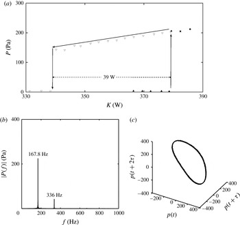
We present the bifurcation diagram depicting the variation of the median value of the peak acoustic pressure with heater power for a mass flow rate of
 $2.34~\text{g}~\text{s}^{-1}$
, in the absence of external noise, in figure 3(a). A clear hysteresis zone and an abrupt jump in the value of acoustic pressure can be observed in the bifurcation plot, which confirms that the bifurcation is subcritical under this condition. Furthermore, the amplitude spectra shows a prominent frequency (figure 3
b) and the reconstructed phase portrait shows an isolated closed orbit, which represents a limit cycle (figure 3
c). The details of phase space reconstruction from experimentally obtained time-series data can be found in Abarbanel (Reference Abarbanel1996) and its application to a thermoacoustic system is presented in Kabiraj & Sujith (Reference Kabiraj and Sujith2012). The subcritical bifurcation observed here is in agreement with the experimental and numerical results reported in the past (Matveev Reference Matveev2003; Balasubramanian & Sujith Reference Balasubramanian and Sujith2008; Subramanian et al.
Reference Subramanian, Mariappan, Sujith and Wahi2010; Juniper Reference Juniper2011; Mariappan Reference Mariappan2011; Gopalakrishnan & Sujith Reference Gopalakrishnan and Sujith2014).
(a) Bifurcation diagram, obtained from experiments, depicting the variation of the median value of the peak acoustic pressure
 $P$
with heater power
 $K$
for mass flow rate
 ${\dot{m}}=2.34~\text{g}~\text{s}^{-1}$
: ▴, forward path; ▿, reverse path. Here, the transition to instability occurs via a subcritical Hopf bifurcation at the heater power
 $K=380~\text{W}$
. (b) The amplitude spectrum of the pressure time series, showing distinct peaks indicating limit cycle oscillations. The bin size used is 0.3 Hz. (c) Phase portrait reconstructed from pressure time series depicting an isolated closed orbit in the phase space. The experiment is conducted in the absence of external noise.

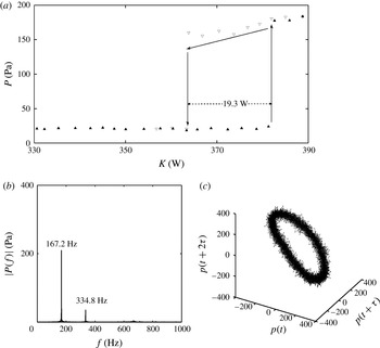
We then performed experiments to investigate the effect of external noise on system dynamics. The bifurcation diagram, amplitude spectra and the reconstructed phase portrait in the presence of external noise of amplitude 10.5 Pa are shown in figure 4(a–c), respectively. It can be seen that the bifurcation remains subcritical in the presence of external noise of amplitude 10.5 Pa. Even in the presence of noise of 10.5 Pa, the change in frequency of oscillations is only 0.6 Hz, which is of the order of the resolution of the FFT. Owing to the presence of noise, the trajectories are spread out, which is indicated by the increased thickness of the limit cycle (figure 4 c). Further, we observe a reduction in the width of the hysteresis zone from 39 W to 19.3 W when external noise is applied.
(a) Bifurcation diagram, obtained from experiments, depicting the variation of the median value of the peak acoustic pressure
 $P$
with heater power
 $K$
, for a mass flow rate of
 ${\dot{m}}=2.34~\text{g}~\text{s}^{-1}$
: ▴, forward path; ▿, reverse path. Here, the transition to instability happens via a subcritical Hopf bifurcation at the heater power
 $K=382~\text{W}$
. (b) The amplitude spectrum of pressure time series, showing sharp peaks indicating limit cycle oscillations. (c) Phase portrait reconstructed from pressure time series, depicting an isolated closed orbit in the phase space. The experiment is performed in the presence of external noise of amplitude 10.5 Pa.

It is worth mentioning that Waugh & Juniper (Reference Waugh and Juniper2011) in their numerical study reported that ‘As the noise strength increases, the system becomes practically unstable further from the Hopf point, increasing the region where triggering may occur. As the noise strength increases further, the system can be dislodged from the stable periodic solution to the zero solution’. Thus, from the work of Waugh & Juniper (Reference Waugh and Juniper2011), it can be inferred that the width of the hysteresis region decreases with increase in the intensity of the applied noise, although they have not stated it explicitly or quantified it. Our observation of the reduction in the width of the hysteresis zone in the presence of Gaussian white noise is the first of its kind in experimental results reported in the thermoacoustic literature. However, outside the context of thermoacoustics, a reduction in the width of the hysteresis zone in the presence of noise is observed in various dynamical systems (Sastry & Hijab Reference Sastry and Hijab1981; Coullet, Elphick & Tirapegui Reference Coullet, Elphick and Tirapegui1985; Geier, Tolstopjatenko & Ebeling Reference Geier, Tolstopjatenko and Ebeling1985; Altares & Nicolis Reference Altares and Nicolis1988; Lekkas, Schimansky-Geier & EngeI-Herbert Reference Lekkas, Schimansky-Geier and EngeI-Herbert1988; L’Heureux & Kapral Reference L’Heureux and Kapral1989; Fedotov, Bashkirtseva & Ryashko Reference Fedotov, Bashkirtseva and Ryashko2002; Berthet et al. Reference Berthet, Petrossian, Residori, Roman and Fauve2003).
We performed experiments at various noise levels for different mass flow rates to confirm the reduction in the width of the hysteresis zone. The noise level is increased with a step size of 1 Pa. Similarly, the variation of non-dimensional hysteresis width with the intensity of additive Gaussian white noise is calculated from the numerical model for different values of time lag
 ${\it\tau}$
. The time lag
 ${\it\tau}$
can be related to the mean flow using Lighthill’s estimate of
 $0.2d_{w}/u_{0}$
, where
 $d_{w}$
refers to the diameter of the heater wire and
 $u_{0}$
refers to the mean flow velocity (Lighthill Reference Lighthill1954; Subramanian, Sujith & Wahi Reference Subramanian, Sujith and Wahi2013).
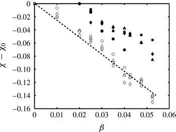
Figure 5 shows the variation of non-dimensional hysteresis width with non-dimensional noise intensity calculated from the experiments and from the numerical model. The non-dimensional width of the hysteresis zone, in the absence of externally added noise, is denoted by
 ${\it\chi}_{0}$
. The uncertainty in non-dimensional hysteresis width
 $({\it\chi}-{\it\chi}_{0})$
is 0.008 and in the non-dimensional intensity of noise is 0.001. Inherent fluctuations are present in the experimental system even in the absence of external noise, and these fluctuations correspond to a non-dimensional noise intensity of 0.02. As a consequence, in figure 5 there are no experimental data corresponding to zero noise intensity. For noise amplitudes up to a threshold, a definite hysteresis zone exists, indicating a subcritical Hopf bifurcation. Nevertheless, the width of the hysteresis zone decreases as the noise intensity increases. We observe a linear decrease in the width of the hysteresis zone with increase in the intensity of the applied noise in results both from experiments and from the numerical model. Further, the rate of decrease is independent of the values of mass flow rates and the values of the time lag.
Variation of non-dimensional hysteresis width (
 ${\it\chi}-{\it\chi}_{0}$
) calculated from experimental and numerical results with non-dimensional noise intensity
 ${\it\beta}$
for different mass flow rates
 ${\dot{m}}$
and for different time lags
 ${\it\tau}$
. The width of the hysteresis zone decreases with increase in noise intensity in both experiments and numerical simulations. The rate of decrease is constant for all mass flow rates and for all time lags. Nevertheless, for the noise levels mentioned here, the transition remains subcritical both in experiments and in numerical simulation. Symbols: ●,
 ${\dot{m}}=2.19~\text{g}~\text{s}^{-1}$
; ▪,
 ${\dot{m}}=2.34~\text{g}~\text{s}^{-1}$
; ▴,
 ${\dot{m}}=2.50~\text{g}~\text{s}^{-1}$
; ♦,
 ${\dot{m}}=2.97~\text{g}~\text{s}^{-1}$
; ○,
 ${\it\tau}=0.2$
; ▫,
 ${\it\tau}=0.175$
; ▵,
 ${\it\tau}=0.15$
; ♢,
 ${\it\tau}=0.125$
.

4.2. Suppression of hysteresis zone in the presence of high-amplitude noise
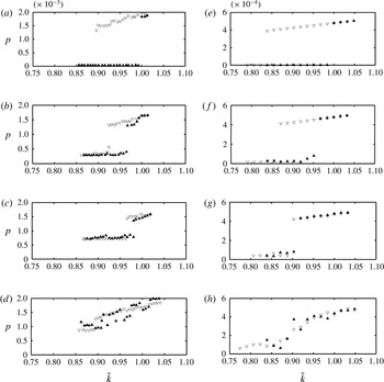
We then proceeded to investigate the effect of high-amplitude noise. Figure 6 represents the variation of non-dimensional acoustic pressure with non-dimensional heater power for different values of non-dimensional noise intensity. Acoustic pressure is made non-dimensional by dividing it by the mean pressure in the case of both experiments and the numerical model. The heater power
 $K$
in experiments is made non-dimensional by dividing it by the value of heater power at the Hopf point in the absence of external noise. In the numerical model, the heater power
 $k$
is non-dimensional to begin with. We normalized the value of
 $k$
by dividing it by the value of the non-dimensional heater power at the Hopf point in the absence of noise.
Bifurcation diagrams obtained from experiments (a–d) and from the numerical model (e–h) depicting the variation of median value of peak non-dimensional acoustic pressure
 $p$
with normalized non-dimensional heater power
 $\tilde{k}$
(normalized by the value of heater power at the Hopf point in the absence of noise) for different values of noise intensities: ▴, increasing
 $\tilde{k}$
; ▿, decreasing
 $\tilde{k}$
. Here,
 ${\it\beta}$
refers to the non-dimensional noise intensity: (a)
 ${\it\beta}=0$
, (b)
 ${\it\beta}=0.15$
, (c)
 ${\it\beta}=0.35$
, (d)
 ${\it\beta}=0.50$
, (e)
 ${\it\beta}=0$
, (f)
 ${\it\beta}=0.025$
, (g)
 ${\it\beta}=0.05$
, (h)
 ${\it\beta}=0.10$
. We can observe a change in the nature of transition and the suppression of the bistable region as the intensity of the external noise increases in the experimental results. Although the pressure amplitudes differ in magnitude, a qualitatively similar behaviour is observed in the case of the numerical model. Note that the ordinates are different.

Figure 6(a–d) represent the changes that happen with increasing noise intensity in experiments. The transition to instability is subcritical in the absence of external noise (figure 6 a). When the non-dimensional noise intensity becomes 0.15, we observe a reduction in the width of the hysteresis zone (figure 6 b). With further increase in the non-dimensional noise intensity to 0.35, there is a further reduction in the width of the hysteresis zone and the transition to instability becomes less abrupt (figure 6 c). When the non-dimensional noise intensity is as high as 0.5, the hysteresis zone is no longer discernible and there is no jump in the value of acoustic pressure (figure 6 d).
Figure 6(e–h) shows the variation of non-dimensional acoustic pressure with non-dimensional heater power for the numerical model for various values of noise intensity. Similar to the experimental results, in the absence of noise, the transition is subcritical (figure 6 e). We observe that the width of the hysteresis zone decreases with increase in noise intensity (figure 6 f). With further increase in noise intensity, the transition starts to become continuous (figure 6 g) and, once the noise intensity becomes high, there is no visible hysteresis zone (figure 6 h). Transition to instability can no longer be termed subcritical as the hysteresis zone is no longer discernible. Even when the transition is continuous there is no perfect overlap between forward and reverse paths (figure 6 f). This is due to the fact that each realization of a stochastic process will be different even when all the system parameters are maintained constant. It is to be noted that, in the case of numerical simulation, qualitatively similar trends with experiments are observed for lower values of non-dimensional noise intensities.
In the presence of high-intensity noise, the system oscillates between a stable oscillatory state and a stable non-oscillatory state. This is referred to as ‘flickering’ in the literature on the critical transitions observed in ecosystems (Scheffer et al. Reference Scheffer, Bascompte, Brock, Brovkin, Carpenter, Dakos, Held, van Nes, Rietkerk and Sugihara2009; Dakos et al. Reference Dakos, Carpenter, Brock, Ellison, Guttal, Ives, Kefi, Livina, Seekell, van Nes and Scheffer2012). This flickering makes the transition continuous and the region of hysteresis becomes indiscernible. The two features that help us to distinguish a subcritical transition are the presence of the hysteresis zone and an abrupt jump in the order parameter (acoustic pressure amplitude in the present case). As these two features become imperceptible beyond a critical noise threshold, we cannot attribute the transition as subcritical. This suppression of the subcritical nature of transition is in complete agreement with the earlier experimental and numerical observations on the effect of noise on nonlinear oscillator models (Sastry & Hijab Reference Sastry and Hijab1981; Juel, Darbyshire & Mullin Reference Juel, Darbyshire and Mullin1997; Zakharova et al. Reference Zakharova, Vadivasova, Anishchenko, Koseska and Kurths2010).
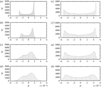
The histograms of the pressure time series, both from experiments and from the numerical model, just at the onset of instability for various values of external noise, are shown in figure 7 to understand the change in the nature of the distribution of pressure values in a single pressure time series. The histogram is constructed by determining the number of data points
 $N$
in the pressure time series having a non-dimensional pressure amplitude
 $p\pm {\rm\Delta}p$
, where
 ${\rm\Delta}p$
refers to the width of the bin. In the absence of external noise, the distribution is bimodal with peaks situated away from the mean. When we increase the intensity of the external noise, there is an increase in the spread of the distribution and a decrease in the height of the peaks. The values near the mean become more probable as the external noise amplitude is increased. Both experimental and numerical results depict the same behaviour. This change in the distribution of the order parameter (acoustic pressure amplitude in our case) in the presence of high-amplitude noise in bistable dynamical systems has been reported outside the context of thermoacoustics (Juel et al.
Reference Juel, Darbyshire and Mullin1997; Deco & Marti Reference Deco and Marti2007). The change from an abrupt transition to a continuous transition in the presence of high-amplitude noise indicates that it will be difficult to identify subcritical transitions that happen in a practical thermoacoustic system working in a turbulent environment.
Histogram of pressure time series at the onset of instability for experimental (a–d) and numerical (e–h) results for various values of noise amplitude. Here,
 ${\it\beta}$
refers to the non-dimensional noise intensity;
 $N$
represents the number of data points in the pressure time series with a non-dimensional pressure
 $p$
; and
 ${\it\psi}^{2}$
represents the variance of the pressure time series: (a)
 ${\it\beta}=0,~{\it\psi}^{2}=0.2428\times 10^{-5}$
; (b)
 ${\it\beta}=0.15,~{\it\psi}^{2}=0.2751\times 10^{-5}$
; (c)
 ${\it\beta}=0.35,~{\it\psi}^{2}=0.2824\times 10^{-5}$
; (d)
 ${\it\beta}=0.50,~{\it\psi}^{2}=0.3083\times 10^{-5}$
; (e)
 ${\it\beta}=0,~{\it\psi}^{2}=0.1363\times 10^{-6}$
; (f)
 ${\it\beta}=0.025,~{\it\psi}^{2}=0.1366\times 10^{-6}$
; (g)
 ${\it\beta}=0.05,~{\it\psi}^{2}=0.1380\times 10^{-6}$
; (h)
 ${\it\beta}=0.10,~{\it\psi}^{2}=0.1402\times 10^{-6}$
. We can see an increase in the spread of the distribution with increase in external noise amplitude, in case of both experimental and numerical results. The increase in the spread is confirmed by the increasing value of variance with increase in noise amplitude. The experimental and numerical results differ in magnitude; however, we intend a qualitative comparison rather than a quantitative one. Note that the abscissas are different by an order of magnitude.

5. Conclusions
In the present work, we study NITs that can happen in a nonlinear system, in the context of a horizontal Rijke tube. We find that even an external noise of amplitude two orders of magnitude less than the limit cycle amplitude can significantly influence the dynamical features of a thermoacoustic system. Our experimental and numerical investigations show that the presence of noise reduces the width of the hysteresis region. The rate of decrease in non-dimensional hysteresis width is linear with noise strength and it is nearly the same for both experimental and numerical results. We observed that the rate of decrease of non-dimensional hysteresis width with noise level is independent of the mass flow rate and the time lag. We find that, in the presence of high-intensity noise, the system exhibits the phenomenon of flickering. This flickering makes the transition continuous and there is a complete suppression of the hysteresis region.
Our study gains significance as most thermoacoustic systems work in noisy environments. Moreover, we have identified the bifurcation characteristics of a prototypical thermoacoustic system in the presence of high-amplitude noise using experimental and numerical methods. To the best of our knowledge, results on the effect of high-amplitude noise on thermoacoustic systems are not found in the literature.
Acknowledgements
This work is funded by ONR Global (Contract Monitors: Drs G. Roy and R. Kolar). We gratefully acknowledge Drs V. Nair, S. T. G. Raghukanth, S. Gupta, S. Sarkar and Ms M. Meenatchidevi for their valuable suggestions and help. We also thank Drs L. Kabiraj and S. Mariappan for the design and fabrication of the experimental set-up and Mr M. Dileesh for help provided in setting up the experiment and in preparing the schematic of the experimental set-up.
Appendix A. Stochastic Runge–Kutta method applied to a general stochastic differential equation
We consider a general stochastic differential equation to show the application of the stochastic Runge–Kutta method to integrate the differential equations in time (Richardson Reference Richardson2009).
Let us consider the general form of an autonomous stochastic differential equation
 $$\begin{eqnarray}\text{d}X(t)=f(X(t))\,\text{d}t+g(X(t))\,\text{d}W(t).\end{eqnarray}$$
Here,
 $X$
represents the dependent variable and
 $t$
represents the independent variable, say time. Functions
 $f$
and
 $g$
correspond to functions of the dependent variable
 $X$
. The second term on the right-hand side of (A 1) represents the noise term, and the noise increment
 $\text{d}W(t)$
is generated from a Wiener process. The value of the dependent variable
 $X(t)$
at any time
 $t$
is given by the expression
 $$\begin{eqnarray}X(t)=X(0)+\int _{0}^{t}f(X(s))\,\text{d}s+\int _{0}^{t}g(X(s))\,\text{d}W(s).\end{eqnarray}$$
Let
 ${\it\delta}t$
be the time step and let
 $L$
be the total number of time steps that we use to numerically integrate (A 2). The value of the dependent variable at any time
 ${\it\tau}_{j}=j{\it\delta}t$
, where
 $j=0,\dots ,L$
, is given by
 $$\begin{eqnarray}X({\it\tau}_{j})=X(0)+\int _{0}^{{\it\tau}_{j}}f(X(s))\,\text{d}s+\int _{0}^{{\it\tau}_{j}}g(X(s))\,\text{d}W(s).\end{eqnarray}$$
Similarly
 $$\begin{eqnarray}X({\it\tau}_{j-1})=X(0)+\int _{0}^{{\it\tau}_{j-1}}f(X(s))\,\text{d}s+\int _{0}^{{\it\tau}_{j-1}}g(X(s))\,\text{d}W(s).\end{eqnarray}$$
If we subtract (A 4) from (A 3), then we will get
 $$\begin{eqnarray}X({\it\tau}_{j})=X({\it\tau}_{j-1})+\int _{{\it\tau}_{j-1}}^{{\it\tau}_{j}}f(X(s))\,\text{d}s+\int _{{\it\tau}_{j-1}}^{{\it\tau}_{j}}g(X(s))\,\text{d}W(s).\end{eqnarray}$$
The second term on the right-hand side of (A 5) can be integrated using the conventional deterministic Runge–Kutta method and we get
 $$\begin{eqnarray}\int _{{\it\tau}_{j-1}}^{{\it\tau}_{j}}f(X(s))\,\text{d}s=\left\{\frac{K_{1}+2K_{2}+2K_{3}+K_{4}}{6}\right\},\end{eqnarray}$$
where
 $K_{1}$
,
 $K_{2}$
,
 $K_{3}$
and
 $K_{4}$
are the increments calculated using the fourth-order Runge–Kutta algorithm.
The third term on the right-hand side of (A 5), which is stochastic, can be obtained using the principles of stochastic calculus. We use Ito’s formulation to integrate the stochastic integral:
 $$\begin{eqnarray}\displaystyle \int _{0}^{T}g(X(t))\,\text{d}W(t) & {\approx} & \displaystyle \mathop{\sum }_{j=0}^{N-1}\left\{\vphantom{\frac{1}{2}}g(X(t_{j}))[W(t_{j+1})-W(t_{j})]\right.\nonumber\\ \displaystyle & & \displaystyle \left.+\,\frac{1}{2}g(X(t_{j}))g^{\prime }(X(t_{j}))[W(t_{j+1})-W(t_{j})^{2}-{\it\delta}t]+\cdots \!\right\}.\end{eqnarray}$$
If the coefficient of the noise term is independent of the state of the system such that
 $g(x)={\it\sigma}$
, i.e. when the noise term is additive in nature, (A 7) changes to
 $$\begin{eqnarray}\int _{0}^{T}{\it\sigma}\,\text{d}W(t)\approx \mathop{\sum }_{j=0}^{N-1}{\it\sigma}[W(t_{j+1})-W(t_{j})].\end{eqnarray}$$
If we substitute (A 8) and (A 6) to (A 5) then we get
 $$\begin{eqnarray}X({\it\tau}_{j})=X({\it\tau}_{j-1})+\left\{\frac{K_{1}+2K_{2}+2K_{3}+K_{4}}{6}\right\}+{\it\sigma}[W(t_{j})-W(t_{j-1})].\end{eqnarray}$$
Thus, we can numerically integrate (A 2) in time to get
 $X(t)$
.