





Nomenclature
- ABC
-
Artificial Bee Colony
- BEMT
-
Blade Element Momentum Theory
- BET
-
Blade Element Theory
- CAMRAD II
-
Comprehensive Analytical Model of Rotorcraft Aerodynamics and Dynamics II
- CFD
-
Computational fluid dynamics
- Coll.
-
Collective pitch
- CPU
-
Central processing unit
- CSD
-
Computational structural dynamics
- DDES
-
Delayed detached-eddy simulation
- deg
-
Degree
- DGW
-
Design gross weight
- EGO
-
Efficient global optimisation
- eVTOL
-
Electric vertical take-off and landing
- FUN3D
-
Fully Unstructured Navier-Stokes Three-Dimensional flow solver
- HART-II
-
Higher Harmonic Control Aeroacoustic Rotor Test II
- HFO
-
High-fidelity optimisation
- HMB3
-
Helicopter Multi-Block 3 CFD solver
- lbf
-
Pound-force
- LFO
-
Low-fidelity optimisation
- MOABC
-
Multi-Objective Artificial Bee Colony
- ms
-
Millisecond
- NASA
-
National Aeronautics and Space Administration
- NFE
-
Number of function evaluations
- NSGA-II
-
Non-dominated Sorting Genetic Algorithm II
- RANS
-
Reynolds-averaged Navier-Stokes
- RMSE
-
Root-mean-square error
- SD
-
Standard deviation
- SLSQP
-
Sequential least-squares programming
- SNOPT
-
Sparse Nonlinear OPTimizer
- UAM
-
Urban air mobility
- UH-60A
-
Sikorsky UH-60A Black Hawk helicopter designation
- XV-15
-
Bell XV-15 tiltrotor research aircraft designation
Roman symbols
- a
-
Two-dimensional lift-curve slope used in the initial collective-pitch estimate (rad⁻¹)
- C d(r)
-
Local sectional drag coefficient
- C d0
-
Zero-lift profile drag coefficient
- C l(r)
-
Local sectional lift coefficient
- C lα, C lα,M(r)
-
Two-dimensional lift-curve slope and its Mach-corrected local value (rad⁻¹)
- C P
-
Rotor power coefficient
- C T
-
Rotor thrust coefficient
- CV λ
-
Coefficient of variation of the induced-inflow ratio (%)
- dC T /dr
-
Sectional thrust-coefficient distribution with respect to nondimensional radius
- E λ
-
Area-weighted standard deviation of the induced-inflow ratio
- f(r)
-
Auxiliary parameter in the Prandtl tip-loss formulation
- f 1, f 2
-
First and second objectives: aerodynamic power coefficient and total root-to-tip blade-twist variation (- / deg)
- fiti
-
Fitness value of candidate solution i
- F(r)
-
Prandtl tip-loss factor
- FM
-
Figure of merit
-
 $\bar{f}$
n, f
n,min, f
n,max
-
Normalised objective n and the minimum and maximum values used for its normalisation (- / native)
- J(X), J total(X)
-
Single-objective cost function and normalised weighted-sum objective function
- k drag
-
Coefficient of the quadratic profile-drag term
- K trim
-
Trim-loop convergence coefficient
- M(r)
-
Local Mach number
- M tip
-
Rotor-tip Mach number
- N
-
Number of radial blade elements
- N b
-
Number of rotor blades
- N s
-
Number of radial stations included in the inflow-uniformity evaluation
- P i
-
Onlooker-bee selection probability for candidate solution i
- p 0
-
Dependent constant coefficient of the fifth-order relative-twist polynomial (deg)
- p 1, …, p 5
-
Independent coefficients of the fifth-order relative-twist polynomial (deg)
- r
-
Nondimensional radial position: local radial coordinate divided by rotor radius
- R
-
Rotor radius (m)
- r local
-
Dimensional local radial coordinate (m)
- ri , rk
-
Nondimensional radial position at blade element or station i or k
- SN
-
Number of food sources or candidate solutions in the ABC colony
- vi,j , xi,j , xk,j
-
Trial, current and comparison-candidate values of design variable j in the ABC neighbourhood search (deg)
- w 1, w 2
-
Weight coefficients in the multi-objective scalarisation, with w1 + w2 = 1
- X
-
Vector of independent twist-polynomial coefficients p5 through p1 (deg)

Greek symbol
- α(r)
-
Local angle of attack (rad in equations; deg when reported)
- α ZLL
-
Zero-lift angle of attack (rad)
- ΔAk
-
Annular-area weighting represented by radial station k
- ΔC d,stall
-
Increment in drag coefficient applied in the separated-flow or stall regime
- Δr
-
Nondimensional radial increment
- Δθ
-
Total root-to-tip blade-twist variation (deg)
- ε trim
-
Thrust-coefficient residual used by the collective-pitch trim loop
-
$\lambda$
(r), λk
-
Local induced-inflow ratio at radial position r or station k
- λi , λi+1
-
Induced-inflow value at blade element i or successive inflow iterates, according to context
-
$\bar{\lambda}$
A
-
Area-weighted mean induced-inflow ratio
- ϕ(r)
-
Local inflow angle (rad)
- ϕi,j
-
Uniformly distributed ABC perturbation coefficient for solution i and variable j, in [−1, 1]
- π
-
Circular constant
- σ(r), σi
-
Local rotor solidity
- θ(r)
-
Local blade pitch angle (rad in equations; deg when reported)
- θ 0,init
-
Initial collective-pitch estimate (rad)
- θ root
-
Blade-root angle; used for the trim pitch setting and for the reported root twist angle (rad in equations; deg when reported)
- θ tip
-
Blade-tip twist angle (deg)
- θ tw
-
Blade-twist term used in the initial collective-pitch estimate (rad)
- θ twist(r)
-
Fifth-order relative-twist distribution (deg)


Subscripts
- 0
-
Zero-lift or constant/base term, according to the parent symbol
- 1, 2
-
First and second objective or associated weighting coefficient
- A
-
Area-weighted quantity
- α
-
Slope or derivative with respect to angle of attack
- b
-
Blade
- best
-
Best-found feasible solution
- d
-
Drag
- drag
-
Quadratic drag-rise model
- i
-
Current iteration, blade element, or candidate-solution index, according to context
- i + 1
-
Next iteration
- init
-
Initial estimate
- j
-
Design-variable index
- k
-
Radial-station index or randomly selected ABC candidate, according to context
- l
-
Lift
- local
-
Dimensional local radial coordinate
- M
-
Mach-corrected quantity
- max
-
Maximum value
- min
-
Minimum value
- n
-
Objective or summation index
- new
-
Updated iteration value
- old
-
Previous iteration value
- P
-
Power
- ref
-
Reference geometry or experimental value
- root
-
Blade-root location or root-pitch setting
- s, S
-
Radial stations
- stall
-
Separated-flow or stall increment
- T
-
Thrust
- target
-
Prescribed target value
- tip
-
Blade-tip location
- trim
-
Collective-pitch trim loop
- tw
-
Blade-twist term in the initial collective estimate
- twist
-
Relative blade-twist distribution
- ZLL
-
Zero-lift line
- λ
-
Statistic associated with the induced-inflow ratio
1.0 Introduction
Rotor blade twist optimisation has long been regarded as an important problem in the aerodynamic design of rotary-wing aircraft. In conventional rotor design, linear or low-degree-of-freedom parametric twist distributions are widely used because of their geometric simplicity and the limited number of design variables they require [Reference Adkins and Liebeck1, Reference Leishman2]. However, local velocity, inflow and sectional aerodynamic loading vary substantially along the rotor span; therefore, a single constant twist gradient may not simultaneously provide aerodynamically favourable loading conditions over the entire span. This consideration makes the investigation of more flexible spanwise twist distributions particularly relevant for rotors of tiltrotor aircraft such as the XV-15 operating at relatively high tip Mach numbers [Reference Leishman2, Reference Seddon and Newman4].
Computational methods with different levels of fidelity have been employed in optimisation studies aimed at improving the aerodynamic performance of rotor blades. High-fidelity computational fluid dynamics (CFD)-based solvers can represent complex three-dimensional rotor-flow structures in greater detail, but impose substantial computational cost when large design spaces require repeated evaluation of many candidate geometries [Reference Johnson3]. In contrast, Blade Element Momentum Theory (BEMT)-based models provide a computationally efficient alternative, particularly for rapid and repeated exploration of the design space [Reference Seddon and Newman4, Reference Glauert and Durand5].
The selection of the optimisation algorithm is also an important consideration in rotor-design problems. Because geometric design spaces may be nonlinear, and aerodynamic evaluations do not always provide derivative information directly, population-based and derivative-free metaheuristic algorithms have been used alongside gradient-based methods in rotor optimisation studies [Reference Johnson and Barakos6, Reference Vu, Lee, Le and Nguyen7]. The artificial bee colony (ABC) algorithm developed by Karaboga employs a population-based search mechanism based on employed, onlooker and scout bee phases [Reference Karaboga8]. Owing to its relatively small number of algorithmic control parameters and its ability to perform derivative-free design-space exploration, ABC was selected in the present study to optimise the coefficients defining the polynomial twist distribution [Reference Karaboga and Basturk9].
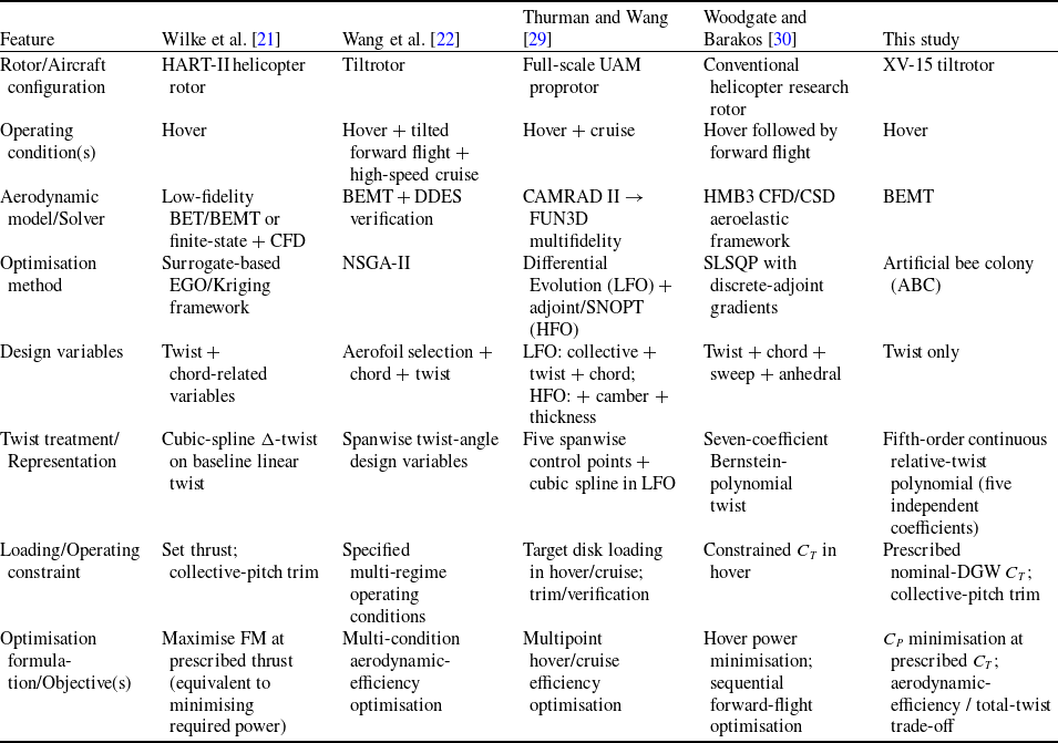
Within this broader methodological context, recent rotor and proprotor optimisation studies show that the design problem has broadened substantially in terms of aerodynamic-model fidelity, design variables and operating conditions. Current approaches range from computationally efficient blade-element/BEMT-based models to high-fidelity CFD/ computational structural dynamics (CSD) and multi-fidelity frameworks. Likewise, blade twist is frequently considered together with chord, aerofoil distribution, collective pitch, rotational speed or other geometric variables, while optimisation problems range from single-point hover designs to multi-regime formulations that include hover, forward flight, transition and cruise [Reference Zeng, Hu, Pan and Shao19, Reference Wilke, Bailly, Kimura and Tanabe21–Reference Ding, Zhang, Peng and Li24, Reference Dayhoum, Ramirez-Serrano and Martinuzzi27–Reference Woodgate and Barakos30]. Within this broader literature, selected recent studies that are directly useful for comparison with the present work and that represent different levels of model fidelity, operating regimes, geometric design spaces and optimisation approaches are summarised in Table 1.
Comparison of representative recent rotor/proprotor blade optimisation studies

Table 1. Long description
Table with multiple columns and rows summarizing recent rotor and proprotor blade optimization studies. Columns include study references, model fidelity, operating regimes, geometric design spaces, and optimization approaches. Each row represents a different study with specific details in each column.
Comparisons in Table 1 show that key methodological elements employed in the present study – prescribed-thrust hover optimisation, smooth or polynomial twist parameterisation and population-based optimisation – have established precedents in the literature [Reference Wilke, Bailly, Kimura and Tanabe21, Reference Wang, Yang, Zhao and Wang22, Reference Thurman and Wang29, Reference Woodgate and Barakos30]. However, a substantial portion of recent work considers twist together with other blade-design variables and/or across multiple operating regimes [Reference Wilke, Bailly, Kimura and Tanabe21–Reference Ding, Zhang, Peng and Li24, Reference Dayhoum, Ramirez-Serrano and Martinuzzi27–Reference Woodgate and Barakos30]. Accordingly, the distinguishing feature of the present study is not any individual methodological ingredient, but their combination within a controlled XV-15 hover problem formulated specifically to isolate the effect of spanwise twist redistribution.
Recent studies not included in Table 1 further support the multi-variable and multi-regime trend. Zeng et al. [Reference Zeng, Hu, Pan and Shao19] considered blade twist together with other rotor-design variables in hover and cruise; Shahjahan et al. [Reference Shahjahan, Gong, Moore and Verstraete23] performed a multivariable optimisation of tilt-wing electric vertical takeoff and landing aircraft (eVTOL) proprotors spanning cruise, hover, and transition; and Ding et al. [Reference Ding, Zhang, Peng and Li24] developed a multi-objective framework for high-altitude proprotor design with combined hover and cruise objectives.
A particularly relevant recent comparison for the XV-15 is provided by Kang et al. [Reference Kang, Park, Cho and Park26]. Using high-fidelity Reynolds-average Navier-Stokes (RANS) calculations for an XV-15 proprotor equipped with optimised aerofoils, the authors compared the baseline geometry with three modified overall-twist cases referenced to 0.75R. In Kang et al. [Reference Kang, Park, Cho and Park26], however, the complete spanwise twist curve was not searched by an optimisation algorithm within a continuous design space; instead, three prescribed modified-twist cases were evaluated parametrically against the baseline geometry. In contrast, the present study represents the entire spanwise twist distribution using a fifth-order continuous polynomial with five independent coefficients, which are optimised directly by the ABC algorithm. Kang et al. [Reference Kang, Park, Cho and Park26] therefore provide an important recent assessment of the influence of twist magnitude on the same XV-15 configuration, while remaining methodologically distinct from the present twist-only stochastic approach in which the full spanwise twist distribution is optimised through a continuous polynomial parameterisation.
The broader rotor-optimisation literature also includes complementary methodological approaches. Lim et al. [Reference Lim, Allen, Haehnel and Dettwiller20] targeted reductions in hover and forward-flight power for the UH-60A but optimised outboard aerofoil-shape parameters rather than blade twist, whereas Sancak [Reference Sancak25] examined different twist distributions using BEMT-based parametric analyses without employing a formal optimisation algorithm. Dayhoum et al. [Reference Dayhoum, Ramirez-Serrano and Martinuzzi27] optimised chord and twist jointly using a genetic algorithm (GA), while Park et al. [Reference Park, Lee, Choi, Kang, Hong, Wilke and Yee28] considered twist and chord within variable- and high-fidelity aerodynamic/structural frameworks for hover and forward-flight objectives. Although older, Gadekar et al. [Reference Gadekar, Abhishek and Kothari31] provide a directly relevant methodological precedent by parameterising both chord and twist distributions with fifth-order polynomial functions and performing blade-element/BEMT-based hover power-loading optimisation. Thus, fifth-order polynomial twist representation is not, by itself, the distinguishing feature of the present work; the distinction lies in the design problem in which the parameterisation is used and in the other design variables deliberately held fixed.
Within this literature context, the present work is formulated as a controlled twist-only design problem intended to isolate the modelled aerodynamic effect of spanwise twist redistribution for the XV-15 rotor at the nominal design gross weight (DGW) hover condition. The chord distribution, aerofoil definition and rotor speed are held fixed, while only the twist geometry is varied using a fifth-order continuous relative-twist polynomial referenced at 0.75R and defined by five independent coefficients. This restricted formulation provides a more controlled basis for relating the modelled performance changes to spanwise twist redistribution from a geometric-design perspective.
The focused design problem is solved at the prescribed isolated-rotor hover thrust corresponding to the nominal DGW condition. The BEMT model used within the optimisation loop is benchmarked against NASA Ames XV-15 hover data, and in the first stage the ABC algorithm minimises C P at prescribed C T . Stochastic repeatability is assessed through 30 independent optimisation runs, so that the best-found solution is characterised across different random initialisations rather than from a single stochastic realisation.
In the second stage, the trade-off between aerodynamic performance and total blade twist is examined within a separate multi-objective design analysis to evaluate the aerodynamic consequences of lower total-twist levels. Studies on composite blade manufacturing have shown that root-to-tip twist and local surface curvature can distort fibre paths during draping, that local fibre-steering geometry can contribute to manufacturing defects and that blade-surface geometry directly influences mould design, tolerancing and demoulding operations [Reference Ho-Nguyen-Tan, Hong, Jaiswal, Oh, Bae, Yu, Kim and Yoon32–Reference Torpan and Zaharia34]. These studies demonstrate that blade twist geometry is a relevant geometric consideration in composite blade manufacturing. Accordingly, total blade twist is retained in the second stage as a geometric design metric associated with manufacturing considerations, and the aerodynamic trade-off associated with reducing this quantity is quantified. Total blade twist is not, however, interpreted here as a direct measure of manufacturability.
Within this framework, the present study complements recent multi-variable and multi-regime optimisation frameworks with a focused XV-15 hover assessment. It provides a bounded and quantitative engineering evaluation of the modelled performance potential attributable to spanwise twist redistribution alone, the stochastic repeatability of the optimisation, and the aerodynamic-performance/overall-twist-demand trade-off at the nominal DGW hover condition.
2.0 Mathematical model and computational methodology
The computational procedure followed in the study is summarised in Figure 1. First, the reference operating conditions for the XV-15 rotor were defined and then the BEMT-based aerodynamic model was developed. The model was validated against NASA Ames experimental data and subsequently employed for the blade twist optimisation [Reference Harris10]. Using the validated model, the aerodynamic performance of different twist distributions was evaluated while maintaining the prescribed target thrust.
Computational methodology and optimisation flowchart.

Each candidate blade twist distribution was parameterised using a fifth-order polynomial and evaluated with the BEMT solver. For each candidate, the induced inflow, sectional aerodynamic loads, thrust coefficient and power coefficient were computed. The trim condition and geometric feasibility were then checked. Candidates failing to satisfy the trim-convergence or geometric-feasibility requirements were handled through penalty terms incorporated into the objective function.
The optimisation loop proceeded by updating the candidate solutions using the ABC algorithm and continued until the prescribed objective-function evaluation budget was reached. For the single-objective optimisation, 30 independent runs were performed, each with a maximum budget of 10,000 objective-function evaluations, and the solution with the lowest final power coefficient among the feasible solutions satisfying the prescribed thrust condition was selected as the best-found solution. In the multi-objective optimisation, the power coefficient and total blade twist were optimised simultaneously to investigate the trade-off between aerodynamic performance and total blade twist.
2.1 Blade Element Momentum Theory (BEMT) and tip loss model
The aerodynamic coefficients of the rotor in hover were predicted using BEMT. In this approach, momentum theory was employed to determine the induced inflow, while blade element theory was used to evaluate the two-dimensional aerodynamic characteristics at each radial blade section. The rotor disk was discretised into a finite number of radial elements, and the local aerodynamic quantities were computed iteratively for each element. The overall thrust and power coefficients were then obtained by integrating the sectional aerodynamic forces along the blade span [Reference Leishman2, Reference Johnson3, Reference Prouty11].
2.1.1 Induced inflow and Prandtl tip loss interaction
The induced inflow ratio (
 $\lambda$
), which varies along the rotor radius, is coupled with the Prandtl tip-loss factor (
 $F$
) which accounts for the reduction of vortex-induced effects near the blade tip [Reference Leishman2]. This condition ensures that the lift generated by the rotor blades approaches zero toward the tip region and is typically solved iteratively. In the present formulation, the momentum balance is applied locally at each annular radial station of the rotor disk. Accordingly, the induced inflow ratio is evaluated as a radially varying local quantity
 $\lambda (r)$
, rather than by prescribing a single uniform inflow value over the rotor disk. The non-dimensional induced inflow ratio at each radial station is given in Equation (1):
 \begin{equation}\lambda \!\left(r\right)=\frac{\sigma \!\left(r\right)C_{{l_{\alpha ,M}}}\left(r\right)}{16F\!\left(r\right)}\left(\sqrt{1+\frac{32F\left(r\right)}{\sigma \!\left(r\right)C_{{l_{\alpha ,M}}}\left(r\right)}\theta \left(r\right)r}-1\right)\end{equation}
The tip loss factor
 $F(r)$
in this equation is calculated using the Prandtl model, as given in Equations (2) and (3), depending on the radial position and the instantaneous induced inflow ratio:
 \begin{equation}f\!\left(r\right)=\frac{N_{b}}{2}\left(\frac{1-r}{\lambda \left(r\right)}\right)\end{equation}
 \begin{equation}F\!\left(r\right)=\frac{2}{\pi }\arccos \!\left(\exp \!\left(-f\left(r\right)\right)\right)\end{equation}
In this approach, Equations (1) and (3) form a coupled local system through the induced inflow ratio
 $\lambda (r)$
and the Prandtl tip-loss factor,
 $F(r)$
. These two quantities are updated successively at each radial station until the relative change between two successive values of
 $\lambda$
satisfies the convergence tolerance defined in Equation (4). The converged local solution is then used for the corresponding blade element before the calculation proceeds to the next radial station.
 \begin{equation}\frac{\left| \lambda _{i+1}-\lambda _{i}\right| }{\lambda _{i}}\lt 10^{-5}\end{equation}
The induced inflow ratio distribution obtained from calculations, varying along the blades as a function of the non-dimensional radius (r/R), is shown in Figure 2.
Radial distribution of induced inflow (8 degrees).

2.1.2 Kinematic relations, compressibility effects, and viscous separation constraints
In BEMT analysis, the local angle-of-attack (
 $\alpha$
) on the blade element is defined as the difference between the local blade pitch angle (
 $\theta$
) and the inflow angle (
 $\phi$
) induced by rotor inflow [Reference Leishman2, Reference Johnson3]. Under the small-angle assumption, the inflow angle and the effective angle-of-attack are given by Equations (5) and (6), respectively:
 \begin{equation}\phi \left(r\right)=\frac{\lambda \left(r\right)}{r}\end{equation}
 \begin{equation}\alpha \left(r\right)=\theta \left(r\right)-\phi \left(r\right)\end{equation}
Due to the design characteristics of the XV-15 aircraft, the high rotor tip Mach number (
 $M_{tip}=0.69$
) makes compressibility significant at the outer radial stations. To model this variation in lift characteristics, the two-dimensional linear lift curve slope (
 $C_{{l_{\alpha }}}$
) was corrected using Equation (7) as a function of the local Mach number
 $M(r)$
in accordance with the Prandtl-Glauert approach [Reference Anderson12].
 \begin{equation}C_{{l_{\alpha ,M}}}\left(r\right)=\frac{C_{{l_{\alpha }}}}{\sqrt{1-M\left(r\right)^{2}}}\end{equation}
Using the corrected aerodynamic slope, the local lift coefficient (
 $C_{l}$
) at each radial station was calculated using Equation (8), with reference to the zero-lift angle-of-attack (
 $\alpha _{ZLL}$
):
 \begin{equation}C_{l}\left(r\right)=C_{{l_{\alpha ,M}}}\left(r\right)\left(\alpha \left(r\right)-\alpha _{ZLL}\right)\end{equation}
After the local lift coefficient is obtained, the profile drag coefficient of the blade element is evaluated. At high angles of attack, a rapid increase in drag is observed due to flow separation over the aerofoil [Reference Anderson12]. The high geometric twist angles near the root region of the XV-15 rotor increase the likelihood of viscous separation in hover conditions. To numerically represent this aerodynamic behaviour, it is assumed that the aerofoil enters the stall regime if the local lift coefficient exceeds the limits of the linear attached-flow region (
 $-0.8\leq C_{l}\leq 1.2$
) [Reference Leishman2]. Accordingly, the local drag coefficient was calculated using an empirical viscous separation model formulated by Equation (9):
 \begin{equation}C_{d}\left(r\right)=\begin{cases} C_{{d_{0}}}+k_{drag}C_{l}\left(r\right)^{2}, &-0.8\leq C_{l}\left(r\right)\leq 1.2\\ C_{{d_{0}}}+k_{drag}C_{l}\left(r\right)^{2}+\Delta C_{d,\textit{stall}} &\quad\qquad \textit{other}\,case \end{cases}\end{equation}
In this equation,
 $C_{d0}$
denotes the profile drag at zero lift,
 $k_{drag}$
is the drag rise coefficient, and
 ${\unicode{x0394}} C_{d,\textit{stall}}$
represents the abrupt increase in viscous drag due to flow separation.
2.1.3 Numerical trim and performance integration
In the final stage of the BEMT analysis, the differential forces calculated on each radial element (
 $r_{k}$
) were numerically integrated along the blade to determine the total rotor performance. The total thrust coefficient and power coefficient of the rotor were numerically summed over the step interval
 ${\unicode{x0394}} (r)$
between the radial stations using Equations (10) and (11), respectively [Reference Leishman2].
 \begin{equation}C_{T}={\sum }_{k=1}^{N}\frac{1}{2}\sigma \left(r_{k}\right)C_{l}\left(r_{k}\right){r}_{k}^{2}{\unicode{x0394}} r\end{equation}
 \begin{equation}C_{P}={\sum }_{k=1}^{N}\frac{1}{2}\sigma \left(r_{k}\right)\left(C_{l}\left(r_{k}\right)\lambda \left(r_{k}\right)+C_{d}\left(r_{k}\right)r_{k}\right){r}_{k}^{2}{\unicode{x0394}} r\end{equation}
In this study, to ensure sufficient numerical accuracy in the first stage, the radial domain was discretised into
 $N=40$
equal elements
 $({\unicode{x0394}} r=1/40)$
.
For the nominal DGW hover condition of the XV-15, the target thrust coefficient was set to (
 $C_{T,\textit{target}}=0.00939$
). This value corresponds to an isolated-rotor approximation in which the 13,000-lbf DGW [Reference Marr18] is equally shared between the two rotors, while wing/airframe download and rotor–airframe interactions are neglected. For each candidate twist distribution, the collective-pitch setting, denoted by
 $\theta _{root}$
in the trim formulation, was adjusted to satisfy this thrust requirement. For this purpose, the initial collective pitch angle was estimated using momentum theory (Equation (12)), and a trim loop was implemented and updated at each iteration. The residual error between the computed and target thrust
 $(\epsilon _{trim}=C_{T,\textit{target}}-C_{T})$
was evaluated, and the collective-pitch setting was updated using Equation (13):
 \begin{equation}{\unicode{x03B8}} _{{0_{init}}}=\frac{6C_{T}}{{\unicode{x03C3}} a}+\frac{3}{2}\sqrt{\frac{C_{T}}{2}}-\frac{3}{4}{\unicode{x03B8}} _{tw}\end{equation}
 \begin{equation}\theta _{root,i+1}=\theta _{root,i}+K_{trim}(C_{T,\textit{target}}-C_{T})\end{equation}
In Equation (13),
 $K_{trim}$
represents the convergence coefficient (
 $K_{trim}=2.5$
). The trim loop was continued until the error fell below the tolerance of
 $10^{-5}$
or the maximum limit of 200 iterations was reached. This approach ensures that the power consumptions of all investigated aerodynamic designs are evaluated in a consistent and comparable manner under conditions where they perform the same lifting task. To verify the physical consistency of the model and boundary conditions, the radial thrust distribution obtained for
 $\theta _{root}=8^{\circ }$
is presented in Figure 3.
Radial distribution of thrust coefficient (8 degrees).

The distribution profile shows that the aerodynamic load is concentrated in the outer region due to the increasing dynamic pressure and decreases at the tip boundary
 $(r\rightarrow R)$
in accordance with physical expectations due to the Prandtl tip loss effect [Reference Leishman2].
2.2 Numerical solution and grid independence
In the developed BEMT model, the total thrust and power coefficients were obtained by numerically integrating the differential aerodynamic forces on the blade. For this purpose, the rotor disk was discretised into a finite number of radial elements. A low number of elements increases discretisation error, whereas excessively high numbers significantly increase computational cost, particularly in optimisation loops. Therefore, a grid independence study was performed to determine an appropriate number of radial elements.
The grid independence analysis performed for the hover condition
 $(\theta _{root}=5^{\circ })$
of the XV-15 rotor is presented in Figure 4. In this study, the number of radial elements was varied between
 $N=10$
and
 $N=100$
. The thrust values predicted by the model were compared with a high-resolution reference solution (
 $N=150)$
, and the relative discretisation error was calculated.
Grid independence and computational cost analysis.

The results show discretisation error is significant for
 $N\lt 30$
range. When the number of elements reaches N = 40, the relative error decreases to approximately 0.3 %. Beyond this value, further refinement yields only marginal improvements in the solution. Increasing the number of elements beyond N = 40 does not provide a significant gain in accuracy, while it increases computational cost. Therefore, N = 40 was selected for all subsequent numerical analyses and optimisation studies.
2.3 Model validation: comparison with NASA experimental data
The XV-15 tiltrotor experimental data published by NASA’s Ames Research Center were used as a reference for the validation of the numerical model. The comparison was performed using the Run 14 data set, which consists of isolated rotor hover tests in which rotor–fuselage interactions are neglected. Consistent with the experimental conditions, the analysis was conducted at standard sea-level conditions where the tip Mach number is
 $M_{tip}=0.69$
[Reference Harris10].
To evaluate the response of the numerical model under different aerodynamic loading conditions, the root collective angle was varied in the range of
 $\,1^{\circ }$
to
 $11^{\circ }$
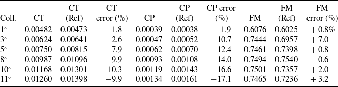
. The resulting thrust coefficient, power coefficient and figure of merit (FOM) values were compared with the experimental data and are presented in Table 2.
BEMT model validation (comparison with NASA XV-15)

Table 2. Long description
A table comparing BEMT model validation with NASA XV-15 data. The table has 7 rows and 10 columns. Column headers are CT, CT, CP, CP error, FM, FM, Coll. CT (Ref) error (%), CP (Ref) (%), and FM (Ref) error (%). Row 1: 0.00482, 0.00473, 0.00039, 0.00038, 0.6076, 0.6025, 1.8, 1.9, 0.8. Row 2: 0.00624, 0.00641, 0.00047, 0.00052, 0.7444, 0.6957, 2.6, 10.7, 7.0. Row 3: 0.00750, 0.00815, 0.00062, 0.00070, 0.7461, 0.7398, 7.9, 12.4, 0.8. Row 4: 0.00987, 0.01096, 0.00093, 0.00108, 0.7494, 0.7540, 9.9, 14.0, 0.6. Row 5: 0.01168, 0.01301, 0.00119, 0.00143, 0.7501, 0.7357, 10.3, 16.6, 2.0. Row 6: 0.01260, 0.01398, 0.00134, 0.00161, 0.7465, 0.7236, 9.9, 17.1, 3.2.
The results in Table 2 show that the numerical model captures the overall aerodynamic trend. The error levels remain limited at low collective angles (
 $\theta _{root}\leq 3^{\circ }$
). In contrast, under medium and high lift conditions (
 $5^{\circ }$
–
 $11^{\circ }$
), the BEMT model underpredicts the thrust by approximately 7–10% compared to the experimental data. The power coefficient is also underpredicted by approximately 12–17%.
The nominal DGW hover target used in the optimisation (
 $C_{T,\textit{target}}=0.00939$
) lies within the loading range examined in the validation and is close to the BEMT result obtained at 8°collective (
 $C_{T}=0.00987$
).
These deviations are primarily attributed to the two-dimensional aerodynamic formulation of the BEMT approach. In particular, three-dimensional flow separation at the rotor root region, tip vortex effects and increased induced drag at high angles of attack cannot be fully captured. As a result, the model predicts lower
 $C_{P}$
and
 $C_{T}$
values at medium and high collective angles relative to the experiments.
When the FOM is considered separately, the discrepancy between the numerical model and the experimental data is smaller compared to the
 $C_{P}$
and
 $C_{T}$
results.
The thrust and power coefficient graphs shown in Figure 5 indicate a systematic underprediction tendency, particularly at medium and high collective angles. In contrast, the FM curve follows the experimental trend more closely over the same range.
Thrust, power and FOM validation plots.

Figure 5. Long description
Panel A: A line graph shows the thrust coefficient (C_T) on the vertical axis, measured in units of 10^-3, against the collective pitch angle on the horizontal axis, measured in degrees. The graph includes two data series: one from the BEMT Model represented by a blue line and another from NASA XV-15 (Experimental) represented by orange squares. The thrust coefficient increases with the collective pitch angle for both data series. Panel B: A line graph displays the power coefficient (C_P) on the vertical axis, measured in units of 10^-3, against the collective pitch angle on the horizontal axis, measured in degrees. The graph includes two data series: one from the BEMT Model represented by a blue line and another from NASA XV-15 (Experimental) represented by orange squares. The power coefficient also increases with the collective pitch angle for both data series. Panel C: A line graph illustrates the figure of merit (FM) on the vertical axis against the collective pitch angle on the horizontal axis, measured in degrees. The graph includes two data series: one from the BEMT Model represented by a blue line and another from NASA XV-15 (Experimental) represented by orange squares. The figure of merit initially increases and then stabilizes as the collective pitch angle increases.
Due to the relationship
 $FM\propto \frac{{C}_{T}^{1.5}}{C_{P}}$
, the error trends in
 $C_{T}$
and
 $C_{P}$
are partially compensated in the FOM calculation. As a result, the deviation in FOM values remains more limited compared to those of the thrust and power coefficients. Within the medium-to-high loading range examined in the validation
 ${5^{\circ }-11^{\circ }}$
, the numerical FOM predictions deviate from the experimental data by approximately 0.6–3.2%.
The
 $C_{T}-C_{P}$
relationship shown in Figure 6 indicates that the model captures the general trend between thrust and power coefficients. Although a relative underprediction is observed in both
 $C_{T}$
and
 $C_{P}$
at medium and high collective angles, the effect of these deviations remains limited in the FOM calculation. These validation results support the use of the BEMT solver for comparative design evaluations within the present low-order framework, while the systematic underprediction observed at medium and high loading remains an acknowledged model-form limitation.
Thrust and power coefficient comparison analysis.

3.0 Optimisation framework and methodology
The BEMT model validated in Section 2 was used as the objective function in the optimisation framework. The numerical solver, which is limited to forward analysis, was embedded into a two-stage metaheuristic optimisation framework to determine the best-found rotor twist geometry. In the first stage, a single-objective ABC algorithm was employed to minimise aerodynamic power consumption under a constant thrust constraint. In the second stage, the framework was extended using a multi-objective artificial bee colony (MOABC) approach [Reference Akbari, Hedayatzadeh, Ziarati and Hassanizadeh15] combined with a Pareto-based solution set to reveal the trade-off between aerodynamic performance and total blade twist.
3.1 Design variables: non-linear twist polynomial
In conventional helicopter blades, linear twist distributions are widely used because of their geometric simplicity; however, they may not provide an aerodynamically favourable twist distribution over the entire blade span under varying local dynamic-pressure conditions [Reference Leishman2]. In the XV-15 aircraft, however, to ensure that blade sections operate at optimal angles of attack corresponding to the varying relative velocities along the radial direction, the blade twist geometry is represented using a fifth-degree polynomial as a function of the non-dimensional radial position
 $r=r_{\text{local}}/R$
[Reference Harris10].
 \begin{equation}{\unicode{x03B8}} _{\text{twist}}\left(r\right)=p_{5}r^{5}+p_{4}r^{4}+p_{3}r^{3}+p_{2}r^{2}+p_{1}r+p_{0}\end{equation}
In Equation (14), the independent decision vector is defined as
 $\boldsymbol{X}=[\,p_{5},p_{4},p_{3},p_{2},p_{1}]$
, while
 $p_{0}$
is determined from the reference condition
 ${\unicode{x03B8}} _{\text{twist}}(0.75)=0$
. Since
 $p_{0}$
is the constant term of the polynomial, it does not affect the spanwise shape or gradient of the twist distribution, but only shifts the entire distribution uniformly. As the overall pitch level is independently adjusted through the collective-pitch trim procedure, treating
 $p_{0}$
as an additional independent design variable would introduce a redundant degree of freedom (DoF). Accordingly,
 $p_{0}$
is evaluated as
 \begin{equation}p_{0}=-\left[p_{5}\left(0.75\right)^{5}+p_{4}\left(0.75\right)^{4}+p_{3}\left(0.75\right)^{3}+p_{2}\left(0.75\right)^{2}+p_{1}\left(0.75\right)\right]\end{equation}
The lower and upper bounds of the five independent polynomial coefficients were defined by applying ±5% variations about their corresponding reference values, with the bound ordering adjusted according to the sign of each coefficient.
3.2 Objective function: power minimisation under constant thrust
The fundamental indicator of hover performance in helicopter and tiltrotor platforms is the shaft power required to meet a specified takeoff weight. Accordingly, the objective function of the proposed optimisation algorithm is defined as the minimisation of the rotor aerodynamic power coefficient
 $C_{P}$
.
Each candidate blade twist geometry generated from the decision variables is evaluated through the aerodynamic equilibrium condition within the BEMT solver prior to power computation. To ensure that the target thrust coefficient corresponding to the nominal DGW hover condition of the XV-15 rotor (
 $C_{T,\text{target}}=0.00939$
) is satisfied, the blade root pitch angle is iteratively updated until the thrust error is minimised. When the rotor disk satisfies the target thrust condition (
 $\mid C_{T}-C_{T,\text{target}}\mid \leq 1\times 10^{-5}$
), the corresponding power coefficient is computed, and the fitness function
 $J(X)$
is evaluated as follows:
 \begin{equation}J\left(X\right)=C_{P}\left(X\right)={\sum }_{i=1}^{N}\frac{1}{2}{\unicode{x03C3}} _{i}\left(C_{l,i}{\unicode{x03BB}} _{i}+C_{d,i}r_{i}\right){r}_{i}^{2}{\unicode{x0394}} r\end{equation}
In Equation (16),
 $N$
denotes the number of blade elements along the spanwise direction [Reference Johnson3]. The optimisation process seeks the parameter set that minimises the cost function defined in Equation (16). Minimising the power coefficient under a constant thrust condition is equivalent to maximising the aerodynamic efficiency of the rotor.
3.3 Artificial bee colony (ABC) algorithm setup
In the aerodynamic optimisation of the rotor blade, the ABC algorithm, a population-based metaheuristic method, was employed to handle the multidimensional search process in the design space [Reference Karaboga8, Reference Karaboga and Basturk9]. The algorithm maintains candidate designs within the prescribed aerodynamic and geometric feasibility criteria while improving the aerodynamic performance of the XV-15 rotor and is based on the collective behaviour of employed, onlooker and scout bees.
The search process is initialised with a population in which each employed bee represents a randomly generated twist polynomial. During the iterative loop, each bee generates a new candidate solution in the neighbourhood of its current position. This exploration in the continuous design space is governed by Equation (17):
 \begin{equation}v_{i,\,j}=x_{i,\,j}+{\unicode{x03D5}} _{i,\,j}\left(x_{i,\,j}-x_{k,\,j}\right)\end{equation}
Here,
 $k$
denotes a randomly selected candidate solution from the population (
 $k\neq i$
), while
 $\phi _{i,\,j}$
is a random coefficient in the range [−1, 1] that controls the magnitude of the search step. Each newly generated blade geometry is evaluated using the BEMT solver, and the resulting aerodynamic power coefficient is transformed into an inversely proportional fitness value for the selection mechanism of the algorithm:
 \begin{equation}{f\kern-1pt it}_{i}=1/\left(1+C_{P,i}\right)\end{equation}
After the employed bees share the fitness values within the colony, the onlooker bees select candidate solutions based on a probabilistic selection strategy
 $P_{i}$
.
 \begin{equation}P_{i}=\frac{{f\kern-1pt it}_{i}}{{\sum }_{n=1}^{SN}\,{f\kern-1pt it}_{n}}\end{equation}
According to Equation (19), the search process is biased toward regions with a higher probability of yielding lower power coefficients. The scout bee mechanism, on the other hand, supports the global exploration capability of the algorithm by abandoning solutions that cannot be improved within the prescribed scout limit of 300 trials.
Because of the stochastic nature of the ABC algorithm, the single-objective optimisation was performed through 30 independent runs. Each run was initialised using a different pseudo-random seed, with a colony size of 50 and a maximum budget of 10,000 number of function evaluations (NFE) per run. The solution yielding the lowest final power coefficient among the feasible solutions obtained from these independent runs was selected as the best-found solution for the subsequent aerodynamic evaluations. The stochastic repeatability of the optimisation and the consistency of the resulting twist distributions are further examined in Section 4.4.1.
The components of the search algorithm constitute the underlying framework of the multi-objective Pareto optimisation, which is presented in detail in Section 3.4.
3.4 Multi-objective optimisation (MOABC) and Pareto approach
In the second optimisation stage, total root-to-tip blade twist,
 ${\unicode{x0394}} \theta =| \theta _{\text{root}}-\theta _{\mathrm{tip}}|$
, was introduced as a second objective in addition to the aerodynamic power coefficient,
 $C_{P}$
. This geometric quantity provides a scalar representation of the overall blade-twist level, enabling a systematic examination of the trade-off between aerodynamic performance and alternative designs with lower total twist. The manufacturing-related physical basis for this choice is supported by composite-blade studies showing that root-to-tip twist and blade geometry are associated with fibre-path development during fabrication and with mould configuration [Reference Ho-Nguyen-Tan, Hong, Jaiswal, Oh, Bae, Yu, Kim and Yoon32, Reference Torpan and Zaharia34]. Nevertheless, manufacturing behaviour also depends on local variables such as surface curvature, fibre paths, steering radius and process conditions [Reference Bakhshi and Hojjati33]; therefore,
 ${\unicode{x0394}} \theta$
is used here as a geometric objective representing total blade twist rather than as a direct measure of manufacturability.
Within this framework, two design objectives are considered simultaneously. The first objective function,
 $f_{1}$
, is the minimisation of the aerodynamic power coefficient,
 $C_{P}$
, whereas the second objective function,
 $f_{2}$
, is the minimisation of the total root-to-tip blade twist variation,
 ${\unicode{x0394}} \theta$
. These conflicting objectives are transformed into a scalar cost function using the weighted sum method [Reference Gunantara13, Reference Marler and Arora14]:
 \begin{equation}J_{\textit{total}}\left(X\right)=w_{1}\cdot \overline{f}_{\!1}\left(X\right)+w_{2}\cdot \overline{f}_{\!2}\left(X\right)\end{equation}
Here,
 $w_{1}$
and
 $w_{2}$
denote the weight coefficients that vary according to design priorities
 $(w_{1}+w_{2}=1)$
, and
 $\overline{f}_{\!n}$
represents the normalisation values that enable objectives with different orders of magnitude to be summed together. The normalisation process was performed by squeezing both objectives between 0 and 1:
 \begin{equation}\overline{f}_{\!n}=\frac{f_{n}-f_{n,min}}{f_{n,max}-f_{n,min}}\end{equation}
The algorithm was run by systematically varying the weighting coefficients, resulting in a Pareto front rather than a single solution. This front represents the trade-off between the aerodynamic power coefficient and total blade twist and defines the non-dominated solution set with respect to
 $C_{P}$
and
 ${\unicode{x0394}} \theta$
[Reference Gunantara13, Reference Marler and Arora14].
Through this approach, the design alternatives presented in Section 4 are based on a consistent analytical framework that supports engineering decision-making.
4.0 Results and discussion
4.1 Single-objective hover performance optimisation
In the first stage of the optimisation process, a constrained single-objective ABC algorithm was employed to evaluate the aerodynamic performance potential of the XV-15 rotor blade under hover conditions. At this stage, the objective function was defined solely in terms of minimising the aerodynamic power coefficient, while total blade twist was not included as a second objective. The optimisation process focused on determining a fifth-order twist distribution that minimises the rotor power coefficient under a constant target thrust coefficient. To represent the nominal design gross weight hover condition of the XV-15, the target thrust coefficient was set to
 $C_{T,\text{target}}=0.00939$
. Under this operating condition, the original XV-15 reference blade evaluated using the BEMT solver yielded a power coefficient of
 $C_{P,\mathrm{ref}}=8.9049\times 10^{-4}$
and an FOM of
 $FM_{\mathrm{ref}}=0.7223$
. During the optimisation, the prescribed aerodynamic feasibility limits and geometric oscillation constraints were enforced. To suppress non-physical radial oscillations that may arise from the mathematical nature of high-order polynomials, undesirable variations in the twist distribution were restricted through a geometric penalty condition applied at the BEMT radial stations. In this way, all candidate geometries were compared under the same target thrust condition and within the same aerodynamic and geometric feasibility criteria.
Among the feasible solutions obtained from the optimisation runs, the configuration with the lowest power coefficient was identified as the best-found solution of the present study. For this geometry,
 $C_{P,\text{best}}=8.1360\times 10^{-4}$
and
 $FM_{\text{best}}=0.7905$
were obtained. Compared with the reference XV-15 geometry at the same target thrust coefficient, the optimised twist distribution resulted in an approximately 8.63% reduction in power coefficient and an approximately 9.45% relative increase in FOM within the present BEMT framework.
As shown in Figure 7, the best-found twist distribution obtained by the ABC algorithm preserves the overall spanwise character of the reference XV-15 geometry while reshaping the twist distribution, particularly in the inboard and mid-span regions. For the resulting geometry, the root twist angle is approximately
 ${\unicode{x03B8}} _{\text{root}}=21.50^{\circ }$
, while the tip twist angle is approximately
 ${\unicode{x03B8}} _{\mathrm{tip}}=-10.94^{\circ }$
, yielding a total root-to-tip twist variation of approximately
 ${\unicode{x0394}} {\unicode{x03B8}} =32.44^{\circ }$
. This value corresponds to a lower total root-to-tip twist than that of the reference geometry. However, because the single-objective optimisation was focused exclusively on reducing aerodynamic power requirement, total blade twist was not treated as an independent optimisation objective at this stage. Therefore, Section 4.2 examines how aerodynamic performance changes as the design is shifted toward lower total blade-twist values within the multi-objective optimisation framework. The resulting MOABC solutions characterise the Pareto trade-off between aerodynamic performance and total blade twist.
Original and optimised twist distribution.

4.2 Multi-objective analysis of aerodynamic performance and total blade twist
Although the single-objective optimisation performed in Section 4.1 successfully reduced the aerodynamic power consumption of the rotor, the trade-off between aerodynamic efficiency and total blade twist requires further evaluation. For this purpose, a MOABC approach was applied, and the relationship between the aerodynamic power coefficient and total twist variation was investigated using the solutions obtained under different weighting combinations. The resulting non-dominated solutions are presented in Figure 8.
Pareto front and search space for aerodynamic power coefficient and total blade twist variation.

As shown in Figure 8, the original XV-15 reference geometry has a power coefficient of approximately
 $C_{P}=0.0008905$
and a total root-to-tip blade twist of 38.45°. The multi-objective optimisation yielded solutions with both lower power coefficients and lower total blade twist than the reference geometry, indicating that the reference design does not lie on the non-dominated boundary with respect to the two objectives considered. For Pareto solutions with greater emphasis on aerodynamic performance, the power coefficient decreases to approximately 0.000814–0.000821, while the total blade twist decreases to approximately 30.8°–32.2°. Relative to the reference geometry, these values correspond to approximately 7.8–8.6% lower power coefficient and 16.3–19.9% lower total blade twist. Toward the lower-twist region of the Pareto front, total blade twist values of approximately 20.8°–21.6° are obtained, corresponding to reductions of approximately 43.8–45.9% relative to the reference geometry; however, the power coefficient increases to approximately 0.000900–0.000907, approximately 1.1–1.9% above the reference value. These results quantitatively characterise the aerodynamic consequences associated with progressively reducing total blade twist. The percentage reductions in total twist characterise the geometric change in the blade, while their significance from a manufacturability perspective should be assessed in the context of the local blade geometry and the specific manufacturing process.
The scattered point cloud represents a representative subset of the feasible intermediate designs evaluated during the optimisation. In the subsequent aerodynamic evaluations of this study, the solution obtained from the optimisation scenario in which aerodynamic performance is fully prioritised
 $(w_{1}=1,w_{2}=0$
) is used as the reference. For this solution, the power coefficient was determined as
 $C_{P}=0.0008136$
, with a total twist of approximately 32.44°.
4.3 Sectional aerodynamic load and inflow distribution of the optimised blade
To examine the radial aerodynamic changes associated with the reduction in power coefficient obtained from the single-objective optimisation, the sectional angle-of-attack and induced-inflow distributions of the reference XV-15 and optimised geometries were compared. Both geometries were evaluated at the same target thrust coefficient,
 $C_{T,\text{target}}=0.00939$
.
As shown in Figure 9, the reference XV-15 geometry reaches relatively high angles of attack of approximately
 $14^{\circ}-15^{\circ }$
in the inboard region, whereas the corresponding peak for the optimised geometry is reduced to approximately
 $9^{\circ}-10^{\circ }$
. The optimised twist distribution provides a more balanced and comparatively more uniform angle-of-attack distribution, particularly over the inboard and mid-span regions. The two distributions approach each other at approximately
 $r/R\approx 0.64$
, beyond which the optimised geometry exhibits slightly higher angles of attack over the outboard region. This behaviour indicates a redistribution of the sectional aerodynamic loading along the blade. In addition, the number of radial stations exceeding the prescribed
 $C_{l}$
limits decreases from 14 for the reference geometry to 2 for the optimised geometry.
Sectional angle-of-attack distribution.

To quantify the change in the induced-inflow distribution, the area-weighted mean, area-weighted standard deviation and coefficient of variation were employed. The area-weighted spatial formulation [Reference Ianniruberto, Astori, Saitta, Milesi, Calle, Gaudino, Girardi, Humphrey, Weinsaft, Votta and Redaelli16] and the use of the coefficient of variation for flow-uniformity assessment [Reference Abattouy, Meslem, Mahdaoui, Ahachad, Guillard, Dappozze, Randrianasolo, Peruchon, Brochier and Lamaa17] were adopted for this purpose. Each BEMT station represents an annular area given by
 ${\unicode{x0394}} A_{k}={\unicode{x03C0}} [(r_{k}+\frac{{\unicode{x0394}} r}{2})^{2}-(r_{k}-\frac{{\unicode{x0394}} r}{2})^{2}]=2{\unicode{x03C0}} r_{k}{\unicode{x0394}} r$
. Because the common factor 2π cancels in the normalised area-weighted expressions, the area-weighted mean induced-inflow ratio is calculated as [Reference Ianniruberto, Astori, Saitta, Milesi, Calle, Gaudino, Girardi, Humphrey, Weinsaft, Votta and Redaelli16]
 \begin{equation}\overline{{\unicode{x03BB}}}_{A}=\frac{{\sum }_{k=1}^{N_{s}}r_{k}\,{\unicode{x03BB}} _{k}\,{\unicode{x0394}} r}{{\sum }_{k=1}^{N_{s}}r_{k}\,{\unicode{x0394}} r}\end{equation}
where
 $N_{S}$
denotes the number of radial stations included in the evaluation,
 $r_{k}$
is the non-dimensional radial position at station
 $k$
,
 ${\unicode{x03BB}} _{k}$
is the corresponding induced-inflow ratio and
 ${\unicode{x0394}} r$
is the non-dimensional radial increment.
 \begin{equation}E_{{\unicode{x03BB}} }=\sqrt{\frac{{\sum }_{k=1}^{N_{s}}r_{k}({\unicode{x03BB}} _{k}-\overline{{\unicode{x03BB}}}_{A})^{2}\,{\unicode{x0394}} r}{{\sum }_{k=1}^{N_{s}}r_{k}\,{\unicode{x0394}} r}}\end{equation}
The coefficient of variation, which represents the relative magnitude of the inflow variation with respect to the mean inflow level, is calculated as [Reference Abattouy, Meslem, Mahdaoui, Ahachad, Guillard, Dappozze, Randrianasolo, Peruchon, Brochier and Lamaa17]
 \begin{equation}CV_{{\unicode{x03BB}} }=100\,\frac{E_{{\unicode{x03BB}} }}{\overline{{\unicode{x03BB}}}_{A}}\end{equation}
Lower values of
 $E_{{\unicode{x03BB}} }$
and
 $CV_{{\unicode{x03BB}} }$
correspond to a more uniform induced-inflow distribution [Reference Ianniruberto, Astori, Saitta, Milesi, Calle, Gaudino, Girardi, Humphrey, Weinsaft, Votta and Redaelli16, Reference Abattouy, Meslem, Mahdaoui, Ahachad, Guillard, Dappozze, Randrianasolo, Peruchon, Brochier and Lamaa17].
Figure 10 shows that the optimised geometry produces a more balanced radial induced-inflow distribution. This trend is also supported by the quantitative results presented in Table 3. The area-weighted standard deviation decreases from
 $9.2277\times 10^{-3}$
to
 $7.6359\times 10^{-3}$
, corresponding to a reduction of approximately 17.25%, while the coefficient of variation decreases from 16.39% to 13.91%, corresponding to a reduction of approximately 15.14%. These results indicate that the optimised geometry provides a more uniform induced-inflow distribution than the reference XV-15 geometry [Reference Ianniruberto, Astori, Saitta, Milesi, Calle, Gaudino, Girardi, Humphrey, Weinsaft, Votta and Redaelli16, Reference Abattouy, Meslem, Mahdaoui, Ahachad, Guillard, Dappozze, Randrianasolo, Peruchon, Brochier and Lamaa17]. The association between a more uniform induced-velocity distribution and a lower induced-power requirement at constant thrust is consistent with momentum theory [Reference Leishman2, Reference Johnson3]. Accordingly, the observed radial redistribution is consistent with the lower power coefficient obtained at the same target thrust coefficient.
Quantitative comparison of induced-inflow uniformity metrics

Table 3. Long description
The table presents a quantitative comparison of induced-inflow uniformity metrics between baseline XV-15 and optimized geometry. It includes three rows and four columns. The columns are labeled as Metric, Baseline XV-15, Optimised geometry, and Change (%). The rows are labeled as Area-weighted mean inflow, Area-weighted standard deviation, and Coefficient of variation. Row 1: Area-weighted mean inflow, 0.05630, 0.05490, 2.49. Row 2: Area-weighted standard deviation, 0.009228, 0.007636, 17.25. Row 3: Coefficient of variation, 16.39 percent, 13.91 percent, 15.14.
Original and optimised induced inflow distribution.

4.4 Design space and algorithm convergence characteristics
This section examines the convergence behaviour and stochastic repeatability of the optimisation process together with the aerodynamic characteristics of the design space. First, the convergence histories obtained from independent ABC runs and the consistency of the resulting blade twist distributions are evaluated. The aerodynamic performance variation within the design space is then examined using two-dimensional cross-sections defined by selected coefficient pairs of the fifth-order twist polynomial. All evaluations were performed at the same target thrust coefficient corresponding to the nominal DGW hover condition.
4.4.1 Convergence behaviour and stochastic repeatability of the ABC optimisation
Because of the stochastic nature of the ABC algorithm, assessing convergence based on a single run is insufficient to characterise the repeatability of the optimisation process. Therefore, 30 feasible runs were performed using the same optimisation settings defined in Section 3.3. The same aerodynamic and geometric feasibility criteria and penalty mechanism were applied in all runs, and each run was conducted with a maximum budget of 10,000 NFEs. In this section, the convergence histories and final objective-function values obtained from the independent runs are evaluated together to assess the stochastic repeatability of the algorithm, followed by an examination of the consistency of the resulting blade twist distributions.
Figure 11 presents the best-so-far power-coefficient histories for 30 independent ABC runs, together with the mean convergence trajectory and the
 $\pm 1\,\mathrm{SD}$
standard-deviation band. A rapid reduction in
 $C_{P}$
is observed during the early stage of the optimisation, accompanied by a marked narrowing of the spread among the independent runs. The inset, focusing on approximately the first
 $1,500\,\mathrm{NFE}$
, provides a more detailed view of this early convergence behaviour. As the search progresses, further improvements in the mean best-so-far value become progressively smaller, and the independent runs approach similarly low
 $C_{P}$
levels. This behaviour indicates that the algorithm repeatedly reaches comparable low objective-function values despite different pseudo-random initialisations.
Convergence behaviour across 30 independent ABC runs.

Figure 11. Long description
A line graph titled ‘Convergence behaviour across 30 independent ABC runs.’ The horizontal axis is labeled ‘Number of Function Evaluations (NFE)’ and ranges from 0 to 10000. The vertical axis is labeled ‘Best-so-Far Power Coefficient, C_P’ and ranges from 8 times 10^-4 to 9.5 times 10^-4. The graph includes multiple lines representing 30 independent runs, a black line indicating the mean best-so-far, and a shaded area showing the mean plus or minus one standard deviation band. An inset zooms in on the early-stage detail, highlighting the initial convergence behavior. The main trend shows a rapid decrease in the power coefficient as the number of function evaluations increases, stabilizing after around 2000 evaluations.
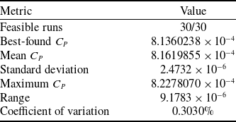
In addition, 27 of the 30 independent runs produced final objective-function values within 1.0% of the best-found solution, further demonstrating the repeatability of the objective-function values across the independent runs. Stochastic repeatability statistics of the 30 independent ABC runs are presented in Table 4.
Stochastic repeatability statistics of the 30 independent ABC runs.

Table 4. Long description
A table with two columns: Metric and Value. The table has 7 rows. Row 1: Metric, Feasible runs; Value, 30/30. Row 2: Metric, Best-found CP; Value, 8.1360238 104. Row 3: Metric, Mean CP; Value, 8.1619855 104. Row 4: Metric, Standard deviation; Value, 2.4732 106. Row 5: Metric, Maximum CP; Value, 8.2278070 104. Row 6: Metric, Range; Value, 9.1783 106. Row 7: Metric, Coefficient of variation; Value, 0.3030 percent.
Figure 12 presents the mean blade twist distribution obtained from the 30 independent runs, together with the
 $\pm 1$
standard-deviation band, the minimum–maximum envelope and the twist distribution of the best-found solution. The geometric variability among the runs is more pronounced in the root and inboard blade regions, while the spread progressively narrows toward the outboard region. The mean spanwise pointwise standard deviation was calculated as 0.8111°, with a maximum pointwise standard deviation of 1.6942° occurring at the blade root. In addition, the root mean square error (RMSE) of the individual run twist distributions relative to the mean twist distribution was 0.8173°. These results indicate that, although the final objective-function values are highly repeatable across the independent runs, a certain degree of geometric variability remains among twist distributions that achieve similarly low objective-function values, particularly in the inboard blade region.
Consistency of blade twist distributions across 30 independent ABC runs.

The repeated convergence of the independent runs to closely clustered low objective-function values provides evidence of stochastic repeatability; however, it does not constitute a mathematical proof of global optimality. Therefore, the final configuration reported in this study is referred to as the best-found solution rather than the global optimum.
4.4.2 Examination of the design space structure and FOM distribution
Representing the blade twist distribution using a fifth-order polynomial results in a multidimensional design space defined by the polynomial coefficients. To visualise how aerodynamic performance varies within this space, two-dimensional cross-sections were constructed for selected coefficient pairs, and the corresponding FOM distributions were examined.
The FOM is defined as [Reference Leishman2]:
 \begin{equation}FM=\frac{{C}_{T}^{3/2}}{\sqrt{2}C_{P}}\end{equation}
 $FM$
varies monotonically and inversely with the power coefficient
 $C_{P}$
under constant-
 $C_{T}$
conditions. Therefore, the
 $FM$
and
 $C_{P}$
surfaces provide equivalent aerodynamic performance rankings, and only the
 $FM$
surfaces are presented to avoid redundant visualisation.
The two-dimensional cross-sections shown in Figures 13 and 14 indicate that the aerodynamic performance does not exhibit the same dependence on different polynomial coefficient pairs. In the
 $p_{4}$
-
 $p_{2}$
plane, relatively high
 $FM$
values are maintained over a broader and more continuous region, whereas in the
 $p_{5}$
-
 $p_{3}$
plane, the high-performance region is concentrated within a narrower range. This behaviour indicates that, within the examined two-dimensional cross-sections, the aerodynamic performance exhibits different sensitivities to different coefficient combinations.
FOM surface for the p4–p2 coefficient pair.

Figure 13. Long description
A 3D surface plot with axes labeled Coefficient p2, Coefficient p4, and Figure of Merit (FM). The plot shows a surface with varying heights and colors, indicating different values of FM for different combinations of p2 and p4. The color scale on the right ranges from blue to yellow, representing FM values from 0.35 to 0.75.
FOM surface for the p5–p3 coefficient pair.

Figure 14. Long description
A 3D surface plot with axes labeled Coefficient p5, Coefficient p3, and Figure of Merit (FM). The plot displays a colored surface representing the figure of merit values across different combinations of coefficients p5 and p3. The color scale ranges from blue to yellow, indicating lower to higher values of the figure of merit. The surface shows a peak around the middle values of p5 and p3, suggesting an optimal region for the figure of merit.
The surfaces presented here represent selected two-dimensional cross-sections of the multidimensional design space. They should therefore be interpreted as complementary analyses of how interactions between the selected coefficient pairs influence the aerodynamic performance distribution, rather than as a complete representation of the entire design space. Within the examined cross-sections, high
 $FM$
values are not distributed uniformly but are concentrated around specific coefficient combinations. These surfaces consequently provide additional insight into the local structure of the aerodynamic performance landscape associated with the optimisation problem.
5.0 Conclusions and future work
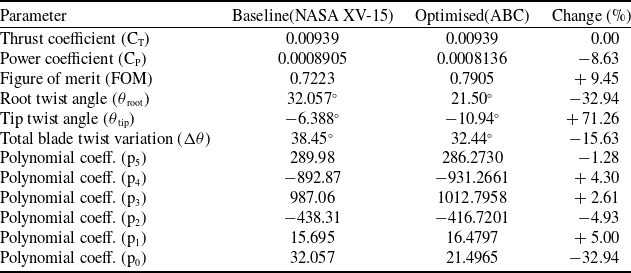
This study investigated the effect of blade twist geometry on the hover performance of the XV-15 tiltrotor. The results reported here are specific to the XV-15 configuration, the nominal hover operating condition considered, and the present BEMT-based modelling framework. Within this scope, the blade twist distribution was found to have a significant influence on the rotor power requirement and aerodynamic efficiency. The effect of the optimised twist geometry on rotor performance is evaluated comparatively with the reference (NASA XV-15) geometry in Table 5.
Baseline and optimised rotor comparison

Table 5. Long description
A table comparing baseline and optimized rotor parameters for the XV-15 tiltrotor. The table has 11 rows and 4 columns. The columns are labeled ‘Metric’, ‘Baseline XV-15’, ‘Optimised geometry’, and ‘Change (%)’. Row 1: Area-weighted mean inflow, 0.05630, 0.05490, -2.49. Row 2: Area-weighted standard deviation, 0.009228, 0.007636, -17.25. Row 3: Coefficient of variation, 16.39 percent, 13.91 percent, -15.14.
Table 5 shows that the best-found twist geometry provides improved predicted aerodynamic performance relative to the reference XV-15 geometry under the same nominal DGW hover thrust condition within the present BEMT framework.
The multi-objective analysis revealed a clear Pareto trade-off between aerodynamic performance and total blade twist. For Pareto solutions prioritising aerodynamic performance, the total blade twist was reduced by approximately 16–20% relative to the reference XV-15 geometry while maintaining a lower power coefficient. Further reductions in total blade twist were accompanied by an increase in power requirement. Thus, the second optimisation stage quantitatively characterised the aerodynamic consequences associated with moving toward lower total blade-twist levels.
Within the scope of future work, the present optimisation framework may be extended to other flight regimes. Accordingly, incorporating forward flight conditions and the asymmetric load distribution that arises depending on the advance ratio into the optimisation will make it possible to expand the model to encompass more realistic flight scenarios.
Additionally, when the computational efficiency provided by the BEMT-based approach and the high accuracy offered by CFD-based analyses are evaluated together, hybrid approaches where these two methods are coupled constitute a significant research direction for future studies.
Acknowledgements
This study was supported by Turkish Aerospace Industries under the Lift Up Project (Award Number: 689f3df12daca). The authors gratefully acknowledge Turkish Aerospace Industries for its financial and technical support.










 Open access

